 Tian Shi
 Yantao Tian
 Zhongbo Sun
 Bangcheng Zhang
 Zaixiang Pang
 Junzhi Yu
 Xin Zhang
95% of researchers rate our articles as excellent or good
Learn more about the work of our research integrity team to safeguard the quality of each article we publish.
Find out more
ORIGINAL RESEARCH article
Front. Neurorobot. , 03 December 2020
Volume 14 - 2020 | https://doi.org/10.3389/fnbot.2020.559048
This article is part of the Research Topic Integrated Multi-modal and Sensorimotor Coordination for Enhanced Human-Robot Interaction View all 17 articles
In this paper, a three-order Taylor-type numerical differentiation formula is firstly utilized to linearize and discretize constrained conditions of model predictive control (MPC), which can be generalized from lower limb rehabilitation robots. Meanwhile, a new numerical approach that projected an active set conjugate gradient approach is proposed, analyzed, and investigated to solve MPC. This numerical approach not only incorporates both the active set and conjugate gradient approach but also utilizes a projective operator, which can guarantee that the equality constraints are always satisfied. Furthermore, rigorous proof of feasibility and global convergence also shows that the proposed approach can effectively solve MPC with equality and bound constraints. Finally, an echo state network (ESN) is established in simulations to realize intention recognition for human–machine interactive control and active rehabilitation training of lower-limb rehabilitation robots; simulation results are also reported and analyzed to substantiate that ESN can accurately identify motion intention, and the projected active set conjugate gradient approach is feasible and effective for lower-limb rehabilitation robot of MPC with passive and active rehabilitation training. This approach also ensures computational when disturbed by uncertainties in system.
The number of limb impairment patients who were injured by stroke has increased year by year, and this disease has also been developing in the direction of youth, seriously endangering the health of patients (Zorowitz et al., 2013). Recently, researchers have paid a great deal of attention to robotics to promote the development of scientific and engineering fields (Jin et al., 2017; Jin and Li, 2018; Xie et al., 2019, 2020; Zhang et al., 2020). Compared to traditional rehabilitation training methods that see problems like resource consumption, high costs, and long rehabilitation period, lower-limb rehabilitation robots can be deemed as a more effective method for recovering patients' movement function. In virtue of interaction generally existing between the lower-limb rehabilitation robot and the patient, to avoid the a second injury in the patient during rehabilitation training, it is essential to propose a human–machine interactive control method, which can be utilized to investigate and analyze the lower-limb rehabilitation robot (Fleischer and Hommel, 2008).
Intention recognition is one of the key points for realizing human–machine interactive control methods with lower-limb rehabilitation robots. Generally, motion intentions include joint angles and angular velocities, which can be recognized by decoding bioelectrical signals. Afterwards, the intentions are referenced by the lower-limb rehabilitation robot to complete interaction (Ding et al., 2016; Peng et al., 2018). An appropriate alternative is to establish a relationship between biological signals and movements for the patient. The surface electromyography (sEMG) can be regarded as the biological signals, which is a micro-electrical signal that appears 20–80 ms before the muscle contraction (Fleischer and Hommel, 2008). Involving two approaches to construct the relationship, one of which is a physiological muscle model, such as the Hill muscle model and the Hammerstein muscle model (Hunt et al., 1998; Buchanan et al., 2004), muscle forces and joint motions can be estimated by those models from sEMG signals; meanwhile, the unidentified physiological parameters of those models affect their applications in rehabilitation systems (Han et al., 2015). Another is the regression model, which can be established to connect sEMG signals to indicate intentions in a straightforward manner, rather than considering physiological parameters (Ding et al., 2016). For instance, a BP neural network was exploited to describe the relationship between sEMG signals and motion intentions, which was verified on able-bodied subjects and patients (Zhang et al., 2012); least squares support vector regression was proposed to predict periodic lower-limb motions from multi-channel sEMG signals (Li et al., 2015). Those approaches constitute a connection between human's bioelectrical signals and motion intentions, and intention recognition can thus be realized effectively.
During the rehabilitation training, the motion trajectory, which is a predetermined curve or recognized by sEMG signals, is known to the rehabilitation device, and the patient is assisted by the lower-limb rehabilitation robot to recover. However, it is very important to avoid the risk of second injury for patients in rehabilitation, and a human–machine interactive control method should therefore be considered to increase security and stability of rehabilitation robots. Recently, some classical control methods have been developed and applied to rehabilitation robots, for example, the rehabilitative system was realized by an adaptive control framework and a human–machine interactive method; meanwhile, the potential conflicts between patient and rehabilitation robot were rejected by position-dependent stiffness and predetermined trajectory (Zhang and Cheah, 2015). Pehlivan et al. (2016) presented a minimal assist-as-needed controller for rehabilitation robots, which could provide corresponding assistance for patients during rehabilitation training.
In recent years, model predictive control (MPC) not only considered the constraints of a non-linear system but predicted future states. People have therefore paid more attention to investigating it and applying it to the aerospace, automobile, economics, and robotics fields. As the patient should be assisted by the lower-limb rehabilitation robot within a relatively safe motion range and protected against accidents, the MPC method is suitable for human–machine interactive control of the lower-limb rehabilitation robot. Generally speaking, the MPC method is designed to optimize multivariable and constrained control systems. On the one hand, a control sequence is created by minimizing an optimization objective function over a finite prediction horizon within state and control constraints. On the other hand, the first optimal solution of non-linear optimization problem feeds back to the non-linear systems, which is utilized to generate the next iteration (Mayne, 2014). A key issue for MPC is that the computational burden of real-time optimization should be reduced through neural networks (Yan and Wang, 2014). To solve this problem is to linearize non-linear systems and discretize the differential term. More and more people have consequently developed some classical methods. For example, a neural network was utilized to identify the unknown non-linear discrete system, and then one-order Taylor expansion formula was used to linearize the MPC problem (Pan and Wang, 2012). For non-linear continuous systems, in order to discretize the differential term and guarantee the higher precision, a Taylor-type numerical differentiation formula was developed and applied to solve non-linear time-varying optimization problem (Zhang et al., 2019), non-linear time-varying equations (Jin et al., 2019), time-varying matrix inversion (Guo et al., 2017), future dynamic non-linear optimization problem (Wei et al., 2019), time-dependent Sylvester equations (Qi et al., 2020), and so on. As the MPC problem can be seen as an optimization problem, a Taylor-type numerical differentiation formula is thus also suitable for solving the MPC problem online.
Another key issue of MPC to be looked at further is online optimization. In fact, an MPC problem can be converted to a non-linear optimization problem with equality constraints and bound constraints and be solved to obtain the control sequence at each sample time. There are thus numerous algorithms proposed and studied for this non-linear optimization problem. A complex-valued discrete-time neural dynamics is studied by Qi et al. (2019) for solving time-dependent complex quadratic programming (QP), which possesses high accuracy and strong robustness but is only suitable for linear constrained QP problems. A trust region-sequential quadratic programming approach attempts to solve a sequence of QP subproblems of non-linear constraint optimization problems, which is based on trust-region technology and applied by finding the Karush-Kuhn-Tucker (KKT) points. It is noteworthy for the approach that the compatibility of the QP subproblem and the Maratos effect were overcome by adding several linear equations into the traditional trust region-SQP algorithm (Sun et al., 2019). However, the calculation of this algorithm is increased by the added linear equations. In addition, some troubles maybe emerge; for instance, one is the consistency of the coefficient matrix and the other the computational burden. Similarly, conjugate gradient methods can also be regarded as an effective optimization approach that utilizes an iteration point with a steep descent direction to generate conjugate direction and compute a global minimum point instead of solving linear equations of trust region-SQP algorithm (Sun et al., 2019). Some classical conjugate gradient methods include the Hestenes-Stiefel (HS) method (Hestenes and Stiefel, 1952), the Fletcher-Reeves (FR) method (Fletcher and Reeves, 1964), the Polak-Ribiére-Polyak (PRP) method (Polak and Ribière, 1969; Polyak, 1969), the Dai-Yuan (DY) method (Dai and Yuan, 2000a), the Liu-Storey (LS) method (Liu and Storey, 1991), and the conjugate descent (CD) method (Dai and Yuan, 2000b), but those methods were exploited to solve unconstrained optimization problems off-line. The MPC problem usually contains some constraint qualifications. Some modified conjugate gradient methods, which consider the constrained conditions, were thus proposed by modifying the search direction and a projected operator (Dai, 2014; Sun et al., 2018). Besides, a projected gradient method, which projected the gradient into the feasible region, was proposed by Rosen (1960), and some modified conjugate gradient methods were extended by some researchers based on the mentioned methods (Li and Li, 2013; Dai, 2014). Those modified conjugate gradient methods were also applied in optimal robust controllers and robots (Sun et al., 2018). In this paper, a modified conjugate gradient method, which will simultaneously consider equality constraints and bound constraints, will be utilized to solve MPC problem. Furthermore, the proposed algorithm of this paper is further applied to the lower limb rehabilitation robots with passive and active rehabilitation.
There are three significant contributions to be developed in this paper. The primary one is that a new projected active set conjugate gradient approach is developed and investigated, and rigorous proof of feasibility and global convergence is also given. The second is that a relationship between sEMG signals and motion intentions established by an echo state network (ESN) model can identify human motion state. Finally, a numerical simulation about passive and active rehabilitation training of lower-limb rehabilitation robot is illustrated and solved by the proposed method. Surprisingly, the studies on the rehabilitation training of lower-limb rehabilitation robot for MPC problem with projected active set conjugate gradient approach are scarce. This motivates our present study.
The rest of this paper is organized as follows: In section 2, the MPC problem is introduced, and a three-order Taylor-type numerical differentiation formula is proposed and utilized to discretize MPC model. In section 3, a new projected active set conjugate gradient algorithm is developed, analyzed, and investigated for the MPC problem, which can be generalized from non-linear systems and lower limb rehabilitation robots. Furthermore, the feasibility and the global convergence of this approach are also proven. The relationship of sEMG signals and motion intentions is established by an ESN model in section 5; meanwhile, passive and active rehabilitation training of lower-limb rehabilitation robot is illustrated and simulated by the proposed method, which is based on sEMG signals with ESN model and MPC problem. Furthermore, the disturbance of dynamic model is also considered through simulation in section 4. Finally, section 6 summarizes the results of lower-limb rehabilitation robot based on the MPC technique and expects future work.
In this subsection, consider the following non-linear control system:
where xk ∈ Rn is a system state variable, uk ∈ Rm is a control input signal, A(xk) ∈ Rn×n, B(xk) ∈ Rn×m, C(xk) ∈ Rn are the state matrix, control input matrix and constant matrix, respectively. yk ∈ Rn denotes the system output, and h(·) is a non-linear function.
MPC for the non-linear control system is devoted to generating a sequence of control signals by minimizing an objective function repeatedly over a finite moving prediction horizon with system state and input constraints satisfied simultaneously. For the non-linear control system (1), the MPC problem can be described as a non-linear discrete-time optimal control problem within input and state constraints:
where r(k + i|k) and y(k + i|k) are the desired output and the predicted output for ith step ahead from kth sampling instant; Δu(k + j|k) = u(k + j|k) − u(k + j − 1|k) denotes the control increment; N and Nu are the prediction horizon and control horizon, respectively; 𝕏k = {x(k + 1|k), x(k + 2|k), …, x(k + N|k)}, ; Q ∈ Rn×n and R ∈ Rm×m are real positive definite matrix, ||·||Q and ||·||R are Euclidean norms defined as , where 𝔄 is a square matrix.
In this subsection, a three-order Taylor-type numerical differentiation formula with truncation error of O(h2) is constructed for the first-order derivative approximation and is exploited to discretize MPC problem (Jin and Zhang, 2014). To obtain the higher-order truncation error, Guo et al. (2017) proposed a novel Taylor-type numerical differentiation formula for the time-varying matrix inversion.
Lemma 1. Assume that xk ∈ C4[a, b] and xk−4, xk−3, xk−2, xk−1, xk, xk + 1 ∈ [a, b], h denotes the sampling gap. Subsequently, a three-order Taylor-type numerical differentiation formula can be obtained as follows:
with a truncation error of O(h3).
Proof. See Guo et al. (2017).
According to the Lemma 1, the non-linear control system (1) can be discreted as
where f = A(x)x + B(x)u + C(x), , , Zk = f(xk, uk) − Gkxk − Bkuk, I is an identity matrix.
Therefore, the MPC problem (2) can be rewritten in the following form:
where xi = x(k + i|k), uj = u(k + j|k), and yi = y(k + i|k), and another symbols see Appendix.
In general, the MPC problem can be solved by the conjugate gradient approach (Šantin and Havlena, 2011), and a sequence
can be regarded as an initial control input sequence of the MPC problem at Step i. In addition, the first element of optimal solution u* can be seen as a feedback control law for non-linear control system (1).
For simplicity, the MPC problem (5) is equivalent to the following non-linear optimization problem with linear equality constrain and bound constrain:
where x = (x, u), Γ(·) is a continuously differentiable function, Λ is a constant matrix, b is a constant vector, and Ω = {x = (x, u)|xmin ≤ x ≤ xmax, umin ≤ u ≤ umax} is a bound constrained set.
In this section, a projected active set conjugate gradient algorithm is proposed to solve the following non-linear optimization problem:
and the convergence of the proposed approach is developed, investigated, and analyzed as follows.
To further analyze projected active set conjugate gradient algorithm, some basic definitions and notions should be revisited in this subsection. Let x* be a stationary point of (7), and consider the following active set:
Furthermore, define
as a set of free variables, where L* is the complement of H*. Therefore, the KKT conditions for the problem (7) can be converted as follows:
where ∇Γi(x) is the ith element of the gradient for Γ at x. According to the literature (Kanzow and Klug, 2006), H(x) and L(x), which approximate the active set and the free variables set can be defined as follows:
where ψ(x) = min{ξ(x), ψ0} and , PΩ(·) is a projection function defined as PΩ(x) = argminω ∈ Ω||x − ω||2. ψ0 is a positive scalar, which should be sufficiently small. Furthermore, it should satisfy the following inequality:
In what follows, let xk be the point of iteration k, and for simplicity, we abbreviate H(xk) and L(xk) as Hk and Lk. According to the literature (Cheng et al., 2014), the active set Hk will be divided into the following three parts:
It is inferred that a search direction dk can be constructed as a feasible direction of Γ at xk if and only if , and , .
It is demonstrated that the active set can be seen as the equality constraints of (7), and according to Rosen's gradient projection method (Rosen, 1960; Dai, 2014), an active set projection matrix is given as follows:
where Ek satisfies and , , ,
Hence the search direction dk is defined by
where
and γ0 is a positive constant. In what follows, the search direction dk can be rigorously proved as a feasible descent direction of Γ at xk for non-linear optimization problem (7).
Theorem 1. Suppose that xk ∈ {x|Λx = b, x ∈ Ω} holds, and xk is not a stationary point of (7), dk is defined by (10), then the search direction dk is a feasible descent direction of Γ at xk for non-linear optimization problem (7).
Proof. According to (8) and (10), and as per definition of the projection matrix, the following two cases can be generalized.
Case 1. If k = 0 or , then the inequality can be directly computed as follows:
Case 2. If k ≥ 1 and ∀i ∈ Lk, then the following inequality can be directly obtained:
The search direction dk is therefore a descent direction of Γ at xk.
Now, the proof of the feasibility for dk is shown as follows, and it is further inferred that
If Ek is not an empty set, it can be seen that
If Ek is an empty set, then Mk = Λ. Owing to Equation (10), then the following equation can be generalized as
If k = 0 or , then
Owing to Equations (13)–(15), then we have Mkdk = 0 for all k ≥ 0. It is also inferred that dk is a feasible descent direction for non-linear optimization problem (7). □
According to the above analysis and investigation, the projected active set HS-type conjugate gradient algorithm (PASHS) is developed, analyzed, and verified for non-linear optimization problem (7).
Algorithm 1. (PASHS)
Step 0. Initialize x0 ∈ {x|Λx = b, x ∈ Ω} and projection matrix 0, let k = 0 and positive constants ε, ψ0, γ0, η0, δ, ρ < 1.
Step 1. If or k > kmax, stop; else go to Step 2.
Step 2. Compute dk by (10).
Step 3. Determine a stepsize by Armijio-type line search rule:
Step 4. Let , and k: = k + 1, go to Step 1.
Remark 1. A projected matrix k is computed by an active set, which ensures iteration point satisfying equality and bounded constraints of non-linear optimization problem (7). Assume that if the component the active set Hk is not contained in the previous iteration point xk, the search direction dk is updated by the second formula of (10); otherwise, the search direction dk is generated by the projected gradient method, which is the first formula of (10). Furthermore, combining with Armijio-type line search, it can be proved that the proposed PASHS algorithm guarantees the feasibility and global convergence for non-linear optimization problem (7).
In this subsection, to further investigate the convergence of the Algorithm 1 (PASHS) for non-linear optimization problem (7), some basic assumptions should be revisited and introduced in this subsection.
Assumption 1. The level set
is bounded.
Assumption 2. Given that the objective function Γ:Rn → R is continuously differentiable on an open set N ⊆ D and its gradient is Lipschitz continuous, there exists a positive constant W > 0 that satisfies the following inequality:
As {Γ(xk)} is a descending sequence, it is clear that the sequence {xk} generated by Algorithm 1 (PASHS) is contained in D. In addition, according to Assumption 1, it is inferred that the gradient of Γ is bounded, i.e., there exists a positive constant γ > 0 such that
Since the matrix is a projected matrix, suppose that there exists a positive constant C > 0, and the following inequality can be obtained:
Lemma 2. Assume that the iterative sequence {xk} generated by Algorithm 1 (PASHS). The step size ηk is obtained via the Armijo line search rule (16), and then there exists a positive constant c0 > 0 such that the following inequality holds
for sufficiently large k.
Proof. According to Armijio-type linear search rule (16), the following inequality can be obtained:
Combined (11) and (12), and the properties of the projected matrix k, the inequality can be generalized as follows
Now, the following two cases can be taken into account and be utilized to prove (21).
Case 1: If ηk = 1, according to Equations (11), (12), and (23), and by applying the Cauchy-Schwarz inequality, we can derive that
Thus, the inequality (21) holds.
Case 2: If ηk < 1, assume that the Armijio-type line search rule is not true, there thus exists a positive constant such that the following inequality holds true:
Using the mean-value theorem and Assumption 1, there exists a positive constant ξk ∈ (0, 1) such that and
Combining inequality (24) and Theorem 1, the following inequality can be directly computed as
Let c0 = min{1, (1 − δ)ρ/W}, the conclusion is true. □
Lemma 3. Suppose that Assumption 2 holds. The iterative sequence {xk} is generated by Algorithm 1 (PASHS), and then the search direction dk defined by (10) is bounded, in other words, there exists a positive constant M ≥ 0 such that
Proof. According to the Assumption 2 and Algorithm 1 (PASHS), the following inequality can be directly obtained:
In addition, in term of the search direction (10) and Theorem 1, the following inequality can be derived as
where is the maximum eigenvalue of the projected matrix k. □
Theorem 2. Suppose that Assumption 1 holds. The iterative sequence {xk} is generated by Algorithm 1 (PASHS), and then
Proof. According to (21), there exists a positive constant c0 such that
Combining Algorithm 1 with Lemma 3, it implies that
The following inequality can be generalized as k → ∞,
Hence . □
Remark. Owing to Theorem 2, it can be seen that the Algorithm 1 (PASHS) is globally convergent for the non-linear optimization problem (7). Combing the ESN learning algorithm and Algorithm 1 (PASHS), the optimal controller of the MPC problem can thus be solved rapidly; this is used for the patients through a lower-limb rehabilitation robot with passive and active rehabilitation training.
In this section, the proposed PASHS algorithm with MPC technique is applied to the passive rehabilitation training of the two-link lower-limb rehabilitation robot. Moreover, combining the ESN model and intention recognition, the MPC and PASHS algorithm also are utilized to active rehabilitation training.
The general dynamic model of two-link lower-limb rehabilitation robot is shown as follows (He et al., 2015):
where q, , are angle, angular velocity and angular acceleration of hip and knee, respectively; τ ∈ R2 is a torque for the rehabilitation robot, which represents admissible control inputs; D(q) ∈ R2×2 is a positive-definite inertia matrix; is a centrifugal and Coriolis term; and G(q) ∈ R2 is related to gravity term. The state space expression of (32) can be described as
where y ∈ R2 is the end-effector position coordinates, h(·) is a function mapping angles of the rehabilitation robot to the position coordinates. The schematic of a two-link lower-limb rehabilitation robot is shown in Figure 1.
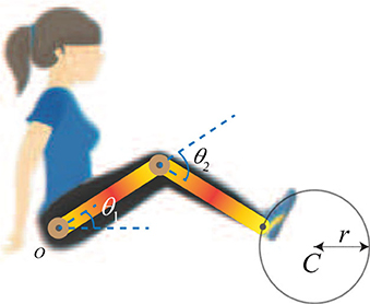
Figure 1. The schematic of two-link lower-limb rehabilitation robot.
As shown in Figure 3, θ1 = q1, θ2 = q2, C and r represent the the hip joint angle, the knee joint angle, center, and radius of the reference trajectory (which can be defined as a circle), respectively. The lengths of the links are l1 = 0.35 m and l2 = 0.32 m; the mass and inertia of two links are m1 = 1.8 kg, m2 = 1.65 kg and kg·m, kg·m, respectively; the gravity constant is g = 9.801 m/s2. In addition, the center and radius are C = (0.5, 0) and r = 0.1 m, respectively.
The parameters of the algorithm 1 (PASHS) are chosen as follows:
and the initial step size is selected as (Dai, 2011)
Due to the proposed MPC model in section 3, the parameters of the MPC will be defined as follows:
the prediction horizon is N = 5 and the control horizon is Nu = 5; the sampling time is h = 0.01s. The initial state of end-effector position coordinates is y0 = (0.6, 0), and the motion-task duration is 25 s with 5 s per cycle. The following experiments are conducted under different constraints of torque: while the hip joint angle and the angular velocity are constrained in interval , and [−π, π], the knee joint angle and the angular velocity are constrained in interval , and [−π, π] (Jin and Zhang, 2011).
Example 1: Consider the following control torques constraints
where τ1 and τ2 correspond to the torques of the hip joint and the knee joint of a two-link lower-limb rehabilitation robot, respectively. The numerical results of this situation are shown in Figures 2–4.
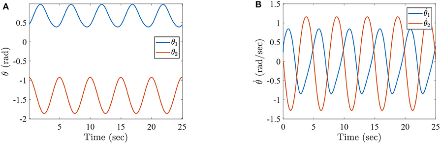
Figure 2. The simulation results with passive rehabilitation training, (A) the angles of lower-limb rehabilitation robot with constraints (34), and (B) the angular velocities of lower-limb rehabilitation robot with constraints (34).
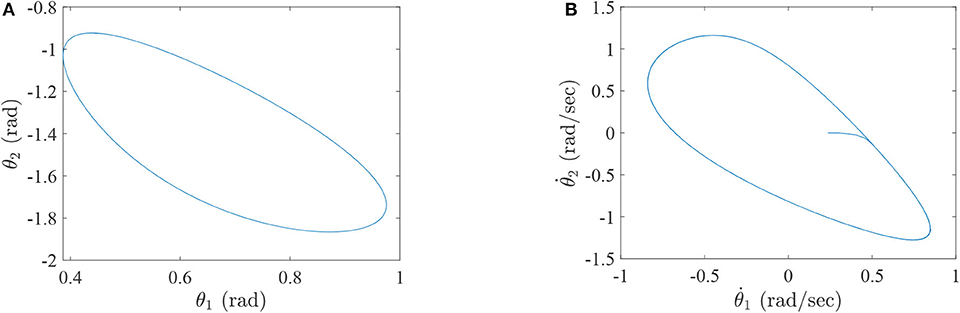
Figure 3. The simulation results with passive rehabilitation training, (A) the phase portraits for angles of lower-limb rehabilitation robot with constraints (34), (B) the phase portraits for angular velocities of lower-limb rehabilitation robot with constraints (34).
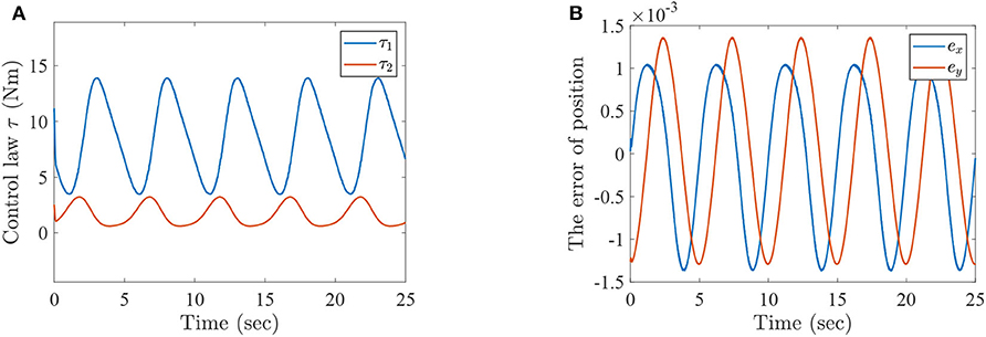
Figure 4. The simulation results with passive rehabilitation training, (A) the torques of lower-limb rehabilitation robot with constraints (34), and (B) the tracking errors of lower-limb rehabilitation robot with constraints (34).
Figure 2 represents the curves of angle and angular velocities of the hip and knee for the two-link lower-limb rehabilitation robot, and Figure 3 is the limit cycles of angle and angular velocities. From Figures 2, 3, it is further inferred that the angles and angular velocities of the lower-limb rehabilitation robot present the periodic properties; it also verifies that the proposed approach is feasible and effective. Figure 4A denotes the control torque vs. time, and the hip joint and knee joint of the rehabilitation robot can be controlled by torques τ1 and τ2, respectively. As shown in Figure 4A, it can be seen that the control torques change periodically for two-link lower-limb rehabilitation robot, which can help the injured patients to do rehabilitation training stably via Algorithm 1 (PASHS) with MPC technique. Figure 4B represents the tracking errors of the real position of end-effector and desired trajectory, while ex and ey are the tracking errors of horizontal ordinate and longitudinal coordinates. As shown in Figure 4B, the absolute value of the tracking errors is also smaller than 0.002 m, which also infers that the lower-limb rehabilitation robot could implement the passive rehabilitation training efficiently by the desired trajectory and MPC technique. It thus further demonstrates that the theoretical analyses are feasible and reliable. Besides, it is very important to take into consideration the energy consumption of rehabilitation training in real-world rehabilitation implementations, therefore, control torques should be constrained within relatively reasonable bounds. As shown in Figure 4A, the optimal control input is obtained by online solving of the MPC problem via Algorithm 1 (PASHS). However, it can be seen from Figure 4A, that the bounded condition is too large for non-linear optimization problem with MPC model, that is, the real-time control torque τ1 is around 13 N·m. In other words, to achieve the low-energy consumption, the boundary constraints can be reduced to around 10 N·m, which are utilized to control the two-link lower limb rehabilitation robot to realize the rehabilitation cycle movement of the injured lower limb.
Example 2: Consider the following control torques with constraint conditions
The numerical results of this situation are shown in Figures 5–7.
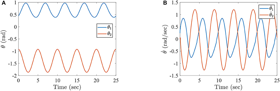
Figure 5. The simulation results with passive rehabilitation training, (A) the angles of lower-limb rehabilitation robot with constraints (35), and (B) the angular velocities of lower-limb rehabilitation robot with constraints (35).
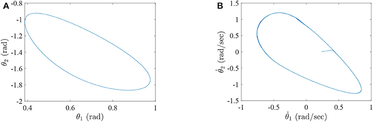
Figure 6. The simulation results with passive rehabilitation training, (A) the phase portraits for angles of lower-limb rehabilitation robot with constraints (35), and (B) the phase portraits for angular velocities of lower-limb rehabilitation robot with constraints (35).
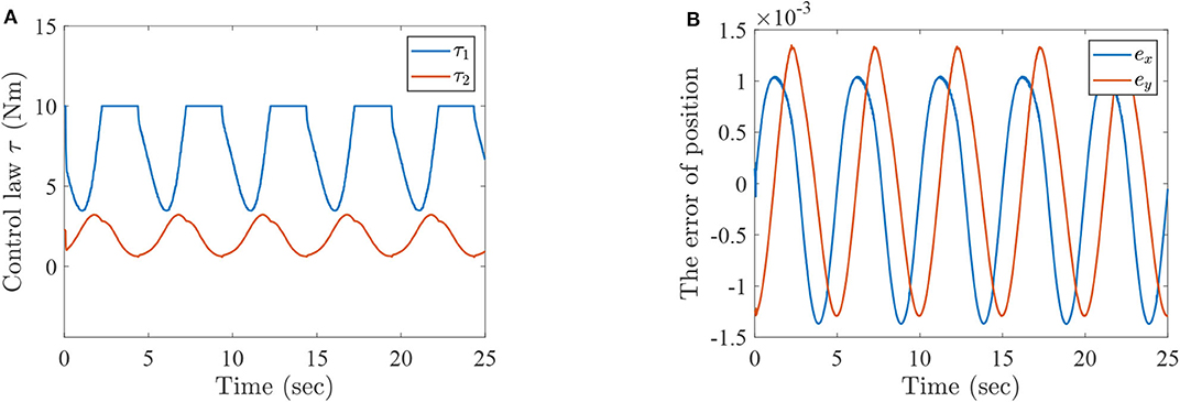
Figure 7. The simulation results with passive rehabilitation training, (A) the torques of lower-limb rehabilitation robot with constraints (35), and (B) the tracking errors of lower-limb rehabilitation robot with constraints (35).
Figure 5 represents the curves of angle and angular velocities for the two-link lower-limb rehabilitation robot, and Figure 6 shows the limit cycles of angle and angular velocities, respectively. As can be seen from Figures 5, 6, the angular velocities of the lower limb rehabilitation robot are affected by the control torques with constraint conditions limited to −10–10 N·m. However, the injured limb can stably complete rehabilitation training activities via the algorithm 1 (PASHS) with MPC technique. Figure 7A shows the control torque vs. time, and it can be seen that the control input τ1 could be constrained in between −10 and 10 N·m, and the smoothness of angular velocities maybe influenced by the constraint conditions. However, it further infers that the stability can be maintained for the two-link lower limb rehabilitation robot. Figure 7B plots the tracking errors of the real trajectories of end-effector and desired trajectories, while ex and ey are the same with the definition of Example 1. The proposed approach is therefore suitable for passive rehabilitation training of lower-limb rehabilitation robot.
Example 3: This example shows a comparison of different algorithms with the MPC solution.
In order to compare the advantages of PASHS algorithm, sequential quadratic programming (SQP) is selected to compare with our algorithm (Sun et al., 2020). The simulation problem is chosen as example 1, and the results are as follows:
Figure 8A represents the horizontal ordinate tracking errors ex of lower-limb rehabilitation robots with passive rehabilitation training, and Figure 8B means the longitudinal ordinate tracking errors ey. From those two figures, it can be seen that the tracking errors of SQP are almost > 0.1 m at every iteration, and sometimes the errors were closed to 1m. This is because an optimal solution for SQP may not be in a feasible region. However, the tracking errors of PASHS are always smaller than 0.01 at every time. The optimal solution of the PASHS algorithm was satisfied by the constraint conditions because of the projective matrix and active set. PASHS was therefore more suitable for the MPC of lower-limb rehabilitation robots. Figure 8C is the running time of two algorithms at every optimization; according to this figure, the running time of PASHS was nearly always smaller than 0.2 s, and the SQP running time was around of 0.4 s. This can account for the real-time computing capability of PASHS algorithm with the MPC technique.
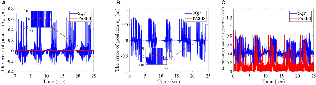
Figure 8. The simulation results with PASHS and SQP, (A) the tracking errors of horizontal ordinate, (B) the tracking errors of longitudinal coordinates, and (C) the running time of algorithm at every time.
Example 4: The example with parameters' perturbation 1.5 times.
This example is reported the influence of uncertainties in system, and the 1.5 times parameters' perturbation is introduced into lower-limb rehabilitation robots. During the simulation, the parameters are selected as l1 = 0.35 m, l2 = 0.32 m, m1 = 2.7 kg, m2 = 2.475 kg, I1 = 0.0827 kg·m, and I2 = 0.0634 kg·m. Other conditions are the same as Example 1. The results of this example are shown as follows.
Figures 9A,B represent the angles and angular velocities of lower-limb rehabilitation robot with 1.5 times parameters' perturbation, respectively. As can be seen from these figures, the angles and angular velocities are changed periodically and stably, although the model is disturbed. Figure 10A is the torques of lower-limb rehabilitation robot which is subjected to 1.5 times parameter perturbation, and Figure 10B represents the horizontal ordinate tracking errors ex and the longitudinal ordinate tracking errors ey of lower-limb rehabilitation robots with 1.5 times parameters' perturbation. From Figure 10A, we can find that torques are limited between −15 and 15 N·m because the mass of lower-limb rehabilitation robot is added. However, the absolute value of tracking errors are smaller than 0.0015 m according to Figure 10B. The PASHS algorithm could thus solve MPC problems of the lower-limb rehabilitation robot with uncertainties in the model, and high accuracy could also be guaranteed.
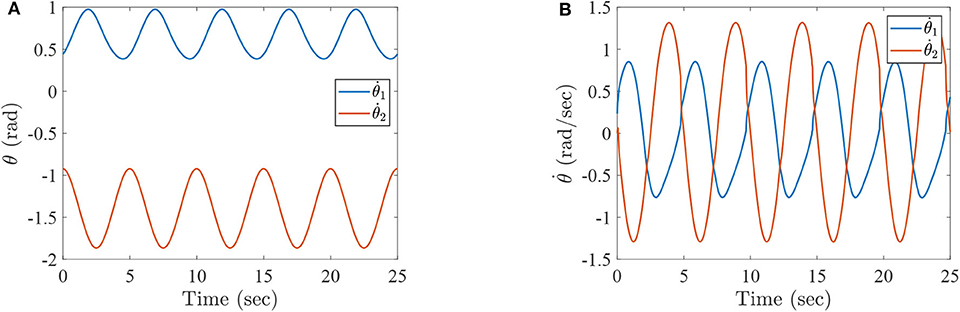
Figure 9. The simulation results with 1.5 times parameters' perturbation, (A) the angles of lower-limb rehabilitation robot with constraints (34), and (B) the angular velocities of lower-limb rehabilitation robot with constraints (34).
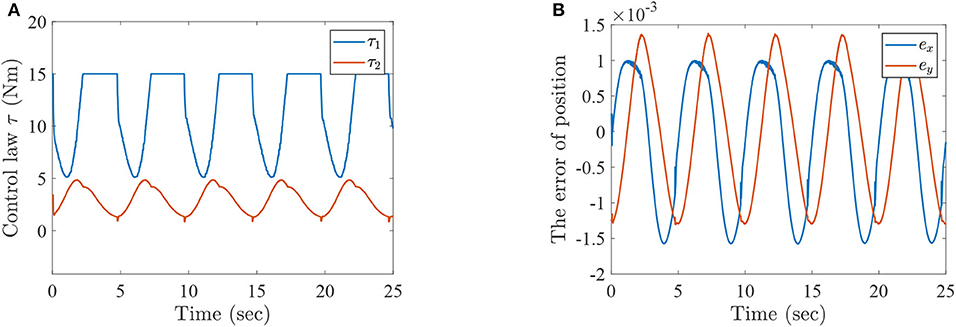
Figure 10. The simulation results with 1.5 times parameters' perturbation, (A) the torques of lower-limb rehabilitation robot with constraints (34), and (B) the tracking errors of lower-limb rehabilitation robot with constraints (34).
In this subsection, the active intention of injured patients is regarded as one of the most important rehabilitation steps. Furthermore, the joint trajectories of injured lower limb can be identified via the mentioned ESN model based on the active motion intention, which can be seen as the desired trajectories of lower limb rehabilitation robots. A numerical simulation is illustrated and analyzed for two-link lower limb rehabilitation robot with ESN model and MPC technique. The technical diagram of sEMG-based active rehabilitation training and intention recognition is shown in Figure 11.
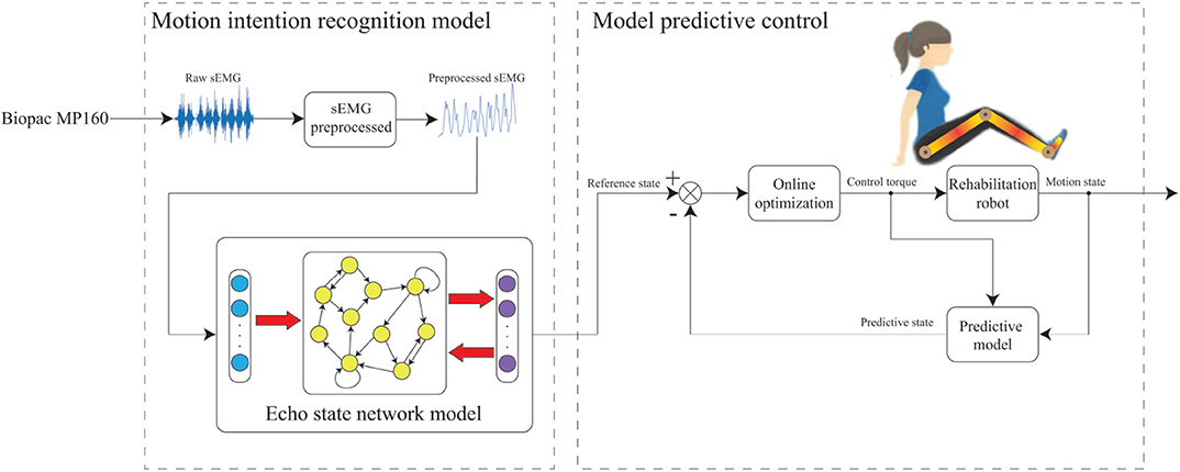
Figure 11. The flowsheet of intention recognition and rehabilitation training.
The active rehabilitation training consists of two parts. The first one is intention recognition, which collects and preprocesses raw sEMG signals, and then motion intention is identified by the ESN model. The details of first part is described in the following description.
During the data acquisition stage, a subject sits on a chair and swings the shank periodically. The sEMG signals of seven muscles of leg, which include the vastus rectus muscle (VR), semitendinosus muscle (SM), tibialis anterior muscle (TA), gastrocnemius muscle (GM), vastus lateralis muscle (VL), biceps muscle of thigh (BM), and extensor pollicis longus (EP), need to be recorded through data acquisition unit, respectively (Tong et al., 2014). The acquisition device is BIOPAC MP160, which can simultaneously capture eight channels of sEMG signals at the default 2 kHz sample rate. Angles and angular velocities of knee and ankle are recorded by inertial measurement unit (IMU), which selects 100 Hz as the sample rate. Due to the sample rate of sEMG signals is higher than IMU, the sub-sampling technology should be implemented by (Zhang et al., 2012)
where sEMGpre(k) represents the sEMG signals after sub-sampling at k times. The position of the electrodes and raw sEMG signals are shown in Figure 12.
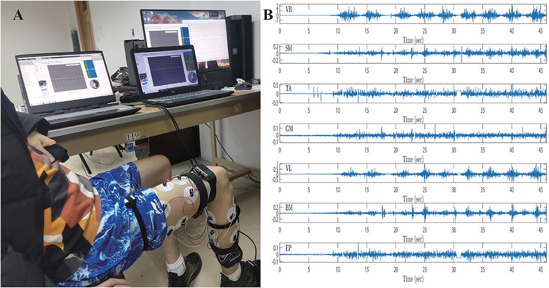
Figure 12. The intention recognition experiment, (A) the sEMG signals sampling of the experiment procedure, (B) the raw sEMG signals of subject.
We then use neural network technology to establish the relationship between sEMG signals and motion state. This is due to the original sEMG signals being contaminated by different measurement noises, such as direct current bias and baseline noise (Law et al., 2011). The raw sEMG signals need to be preprocessed, which includes a high-pass filter with 50 Hz high cut-off frequency, full-wave rectification technology, low-pass filter with 5 Hz low cut-off frequency and normalized technology (Han et al., 2015). The sEMG signals can be seen as the input signals of neural network when the noise of raw sEMG signals is eliminated by the mentioned methods.
The ESN model is a kind of recurrent neural network that is composed of an input layer, a hidden layer where neurons interconnect randomly, and an output layer. The network architecture is depicted in Figure 13.
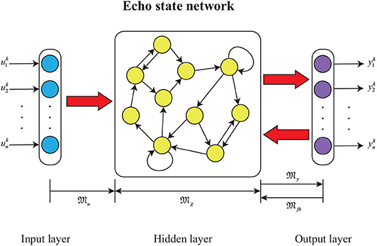
Figure 13. The ESN diagram.
The mathematical model of the ESN model can be obtained as
where is an activation function and commonly generates from ; , , , are the internal connection weight of the hidden layer, the input layer to the hidden layer connection weight matrix, the output layer to the hidden layer feedback weight matrix, and the hidden layer to the output layer connection weight matrix; and are the echo state and output vectors of the ESN model, respectively. Assume that , , and are unmodifiable during the ESN model training (Pan and Wang, 2012). The ESN algorithm with off-line learning is summarized as follows.
Algorithm 2. (ESN learning algorithm)
Step 0. Initialize echo state and randomly obtain a matrix 𝔐. Normalize and generate , , , where is a spectral radiuses of and |λmax| is a spectral radius of 𝔐.
Step 1. Compute the echo state by
for k = 0, 1, …, N, where and are the kth input and output reference data from the training dataset.
Step 2. Collect the reservoir state X and target state Y as follows:
Step 3. Off-line compute matrix , where X+ is the pseudo-inverse of X.
During the training process, the preprocessed sEMG signals are recorded by the Biopac MP160 system with seven channels from 0 to 46 s. Furthermore, the joint trajectories of injured lower limb are recorded by IMU, the data set from 0 to 32 s is then collected as a training set, and the remainder of the data set is regarded as a test set. The training set is utilized to train the ESN model, and the testing set is exploited to simulate lower limb rehabilitation robots with active rehabilitation training. The real angles and angular velocities are recorded by IMU, which aims at demonstrating the accuracy of proposed method. The ESN model has seven input neurons and four output neurons, the numbers of ESN hidden layer neurons are 100, and the parameters are selected as follows: . The results of ESN training and testing are shown in Figures 14, 15.
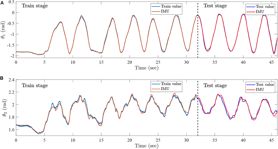
Figure 14. Intention recognition results for angles, (A) the knee angle, which is recognized by the sEMG and ESN model, and (B) the ankle angle, which is recognized by sEMG and ESN model.
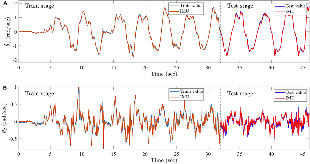
Figure 15. Intention recognition results for angular velocities, (A) the knee angular velocity, which is recognized by sEMG and ESN model, and (B) the ankle angular velocity, which is recognized by the sEMG and ESN model.
Figure 14 represents the intention recognition results of injured lower limb via ESN model, where θ1 and θ2 mean knee and ankle angles, respectively. Red solid lines denote real joint trajectories of knee and ankle angles, and blue solid lines represent training and testing results of ESN learning algorithm. Figure 15 shows the training and testing results of knee and ankle angular velocities through ESN learning algorithm. and mean the angular velocities for knee and ankle, which are shown by blue solid lines. Red solid lines represent real angular velocities, which are recorded by IMU. As can be seen from Figure 14, the injured lower limb swings the calf at the 5th second, and then the knee periodically stretches and flexes about at about 41 s. When the knee joint angle reaches 0 rad, the knee joint swings to its maximum position. During the swing phase, the knee joint can flex more than −1.8 rad. The angle of the ankle joint is between 1.8 and 2.2 rad, which is always plantar flexion. Figure 15 shows that the angular velocity of the knee joint alternates between −2 and 2 rad/s with a cycle of about 4 s, while the angular velocity of the ankle joint varies slightly between −0.5 and 0.5 rad/s. The motion intention of injured lower limbs can be identified by the ESN learning algorithm with multichannel sEMG signals from 32 to 45.3 s. Meanwhile, it is also inferred that the proposed method shows superior performance for intention identification of injured lower limb.
The second one is an MPC problem; the joint trajectories of injured lower limb can be identified via an ESN model based on active motion intention, which is viewed as desired trajectories of the two-link lower limb rehabilitation robot. The control law generated by the Algorithm 1 (PASHS) is transmitted to two-link lower limb rehabilitation robot, which aims at assisting patient to do rehabilitation training. The next predictive state also can be computed by the optimization results of MPC problem (2), which feeds back to the two-link lower limb rehabilitation robot system. Meanwhile, the MPC problem can be seen as follows:
where ki,j ≜ k + i, j|k, and θk, , and τk represent the angle vector, angular velocity vector, and torque vector of two-link lower limb rehabilitation robot at prediction horizon and control horizon, respectively. θd(k + i|k) means the desired trajectory at k + i time, and Δτ(k + j|k) is the control input increment. Q = 5I and R = I, where I is the identity matrix and the index N = 3 and Nτ = 3.
The trained ESN model can effectively identify the joint angle and angular velocity of injured lower limb from the multichannel sEMG signals. The lower limb rehabilitation robot takes the results of recognition as the desired trajectories. Combining the ESN model and MPC technique, the human–machine interactive control method is developed, investigated, and analyzed for lower limb rehabilitation robot and injured lower limb in this paper. Besides, to design the human-machine interactive controller, the joint angle and angular velocity that can be regarded as desired trajectories are identified by ESN learning algorithm from 32 to 46 s. The numerical results are shown in Figure 16.
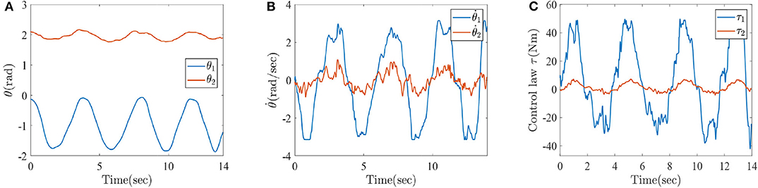
Figure 16. The simulation results with active rehabilitation training, (A) the angles of lower-limb rehabilitation robot based on active intentions, (B) the angular velocities of lower-limb rehabilitation robot based on active intentions, and (C) the torques of lower-limb rehabilitation robot.
Figures 16A–C represent the numerical results of angles, angular velocities, and torques of lower-limb rehabilitation robot during rehabilitation training process. As shown in Figure 16, the blue solid lines mean the results of knee and the red solid lines represent the results of ankle, respectively. In light of Figure 16, it can be seen that the patients can be stably driven to do rehabilitation motion by lower limb rehabilitation robot, which be oriented by a human's active intention. It is also inferred that the rehabilitation robot appropriately generates torques, which assist patients to do rehabilitation training and avoid the second injury. It is thus further demonstrated that it is very practical to train the injured lower limb through a human–machine interactive control method with multichannel sEMG signals. In other words, it is also verified that the ESN learning algorithm and Algorithm 1 (PASHS) are feasible and effective for the rehabilitation training of injured lower limb.
In this paper, to obtain an optimal controller of a non-linear system, an MPC problem firstly solved by a new PASHS algorithm has been proposed and analyzed by exploiting the three-order Taylor discretization formula to linearize and discretize the constraint conditions. Furthermore, the PASHS approach not only takes advantage of a projected operator, but it also integrates the active set into HS conjugate gradient methods; the optimal controller can thus be rapidly solved for a non-linear optimization problem. Moreover, the feasibility and global convergence have been rigorously proved in this paper. Some numerical results have been presented and analyzed to substantiate the feasibility, effectiveness, and superiority of the developed human–machine interactive control method for passive/active rehabilitation training. The ESN model with multichannel sEMG signals also has been proposed for intention recognition, which could identify the joint angles and angular velocities of the injured lower limb to realize active rehabilitation training. In other words, passive rehabilitation makes patients train through fixed-based trajectories of injured lower limb; however, the desired trajectories of active rehabilitation training are identified by ESN learning algorithm with multichannel signals. Besides, combining with MPC technology and Algorithm 1 (PASHS), human-machine interactive control has been developed, investigated, and analyzed for two-link lower limb rehabilitation robot. The numerical results have inferred that the proposed method could be effectively applied to passive/active rehabilitation training. The proposed method has also solved a problem that creates uncertainty in the model. In future work, more effective and real-time methods will be developed and investigated in the solution of MPC problem and applied to the rehabilitation of patients, such as upper limb rehabilitation training, assisting patients to walk on the plane, or up and down stairs.
Publicly available datasets were analyzed in this study. This data can be found at: http://www.dqxy.ccut.edu.cn/2017/0906/c5519a78133/page.htm.
Ethical review and approval was not required for the study on human participants in accordance with the local legislation and institutional requirements. Written informed consent for participation was not required for this study in accordance with the national legislation and the institutional requirements.
TS: methodology, software, and review. YT: investigation and writing original draft. ZS: conceptualization and methodology. BZ: methodology. ZP: algorithm. JY: methodology and review. XZ: editing. All authors contributed to the article and approved the submitted version.
This work was supported in part by the National Natural Science Foundation of China under Grants 61873304, 11701209, and 51875047, and also in part by the China Post-doctoral Science Foundation Funded Project under Grant 2018M641784, 2019T120240, and also in part by the Key Science and Technology Projects of Jilin Province, China, Grant No. 20200201291JC.
The authors declare that the research was conducted in the absence of any commercial or financial relationships that could be construed as a potential conflict of interest.
Buchanan, T., Lloyd, D., Manal, K., and Besier, T. (2004). Neuromusculoskeletal modeling: estimation of muscle forces and joint moments and movements from measurements of neural command. J. Appl. Biomech. 20, 367–395. doi: 10.1123/jab.20.4.367
Cheng, W., Liu, Q., and Li, D. (2014). An accurate active set conjugate gradient algorithm with project search for bound constrained optimization. Optim. Lett. 8, 763–776. doi: 10.1007/s11590-013-0609-6
Dai, Y., and Yuan, Y. (2000a). A nonlinear conjugate gradient method with a strong global convergence property. SIAM J. Optim. 10, 177–182. doi: 10.1137/S1052623497318992
Dai, Y., and Yuan, Y. (2000b). Nonlinear Conjugate Gradient Methods. Shanghai: Shanghai Science and Technology Publisher.
Dai, Z. (2011). Two modified HS type conjugate gradient methods for unconstrained optimization problems. Nonlin. Anal. 74, 927–936. doi: 10.1016/j.na.2010.09.046
Dai, Z. (2014). Extension of modified Polak-Ribière-Polyak conjugate gradient method to linear equality constraints minimization problems. Abstr. Appl. Anal. 2014, 1–9. doi: 10.1155/2014/921364
Ding, Q., Xiong, A., Zhao, X., and Han, J. (2016). A review on researches and applications of semg-based motion intent recognition methods. Acta Autom. Sin. 42, 13–25. doi: 10.16383/j.aas.2016.c140563
Fleischer, C., and Hommel, G. (2008). A human-exoskeleton interface utilizing electromyography. IEEE Trans. Robot. 24, 872–882. doi: 10.1109/TRO.2008.926860
Fletcher, R., and Reeves, C. M. (1964). Function minimization by conjugate gradients. Comput. J. 7, 149–154. doi: 10.1093/comjnl/7.2.149
Guo, D., Nie, Z., and Yan, L. (2017). Novel discrete-time zhang neural network for time-varying matrix inversion. IEEE Trans. Syst. Man Cybernet. Syst. 47, 2301–2310. doi: 10.1109/TSMC.2017.2656941
Han, J., Ding, Q., Xiong, A., and Zhao, X. (2015). A state-space EMG model for the estimation of continuous joint movements. IEEE Trans. Ind. Electron. 62, 4267–4275. doi: 10.1109/TIE.2014.2387337
He, W., Ge, S. S., Li, Y., Chew, E., and Ng, Y. S. (2015). Neural network control of a rehabilitation robot by state and output feedback. J. Intell. Robot. Syst. 80, 15–31. doi: 10.1007/s10846-014-0150-6
Hestenes, M. R., and Stiefel, E. L. (1952). Methods of conjugate gradients for solving linear systems. J. Res. Natl. Bureau Stand. 49, 409–432. doi: 10.6028/jres.049.044
Hunt, K., Munih, M., Donaldson, N., and Barr, F. (1998). Investigation of the hammerstein hypothesis in the modeling of electrically stimulated muscle. IEEE Trans. Biomed. Eng. 45, 998–1009. doi: 10.1109/10.704868
Jin, D., and Zhang, J. (2011). Bio-mechanology in Rehabilitation Engineering. Beijing: Tsinghua University Press.
Jin, L., and Li, S. (2018). Distributed task allocation of multiple robots: a control perspective. IEEE Trans. Syst. Man Cybernet. Syst. 48, 693–701. doi: 10.1109/TSMC.2016.2627579
Jin, L., Li, S., Hu, B., Liu, M., and Yu, J. (2019). A noise-suppressing neural algorithm for solving the time-varying system of linear equations: a control-based approach. IEEE Trans. Ind. Inform. 15, 236–246. doi: 10.1109/TII.2018.2798642
Jin, L., Li, S., La, H. M., and Luo, X. (2017). Manipulability optimization of redundant manipulators using dynamic neural networks. IEEE Trans. Ind. Electron. 64, 4710–4720. doi: 10.1109/TIE.2017.2674624
Jin, L., and Zhang, Y. (2014). Discrete-time zhang neural network of o(τ3) pattern for time-varying matrix pseudoinversion with application to manipulator motion generation. Neurocomputing 142, 165–173. doi: 10.1016/j.neucom.2014.04.051
Kanzow, C., and Klug, A. (2006). On affine-scaling interior-point newton methods for nonlinear minimization with bound constraints. Comput. Optimiz. Appl. 35, 177–197. doi: 10.1007/s10589-006-6514-5
Law, L. F., Krishnan, C., and Avin, K. (2011). Modeling nonlinear errors in surface electromyography due to baseline noise: a new methodology. J. Biomech. 44, 202–205. doi: 10.1016/j.jbiomech.2010.09.008
Li, C., and Li, D. (2013). An extension of the fletcher-reeves method to linear equality constrained optimization problem. Appl. Math. Comput. 219, 10909–10914. doi: 10.1016/j.amc.2013.04.055
Li, Q., Song, Y., and Hou, Z. (2015). Estimation of lower limb periodic motions from semg using least squares support vector regression. Neural Process. Lett. 41, 371–388. doi: 10.1007/s11063-014-9391-4
Liu, Y., and Storey, C. (1991). Efficient generalized conjugate gradient algorithms, part 1: theory. J. Optimiz. Theory Appl. 69, 129–137. doi: 10.1007/BF00940464
Mayne, D. Q. (2014). Model predictive control: recent developments and future promise. Automatica 50, 2967–2986. doi: 10.1016/j.automatica.2014.10.128
Pan, Y., and Wang, J. (2012). Model predictive control of unknown nonlinear dynamical systems based on recurrent neural networks. IEEE Trans. Ind. Electron. 59, 3089–3101. doi: 10.1109/TIE.2011.2169636
Pehlivan, A. U., Losey, D. P., and O'Malley, M. K. (2016). Minimal assist-as-needed controller for upper limb robotic rehabilitation. IEEE Trans. Robot. 32, 113–124. doi: 10.1109/TRO.2015.2503726
Peng, L., Hou, Z., Wang, C., Luo, L., and Wang, W. (2018). Physical interaction methods for rehabilitation and assistive robots. Acta Autom. Sin. 44, 2000–2010. doi: 10.16383/j.aas.2018.c180209
Polak, E., and Ribière, G. (1969). Note sur la convergence de méthodes de directions conjuguées. Rev. Franç. Inform. Rec. Opér. 16, 35–43. doi: 10.1051/m2an/196903R100351
Polyak, B. (1969). The conjugate gradient method in extreme problems. USSR Comput. Math. Math. Phys. 9, 94–112. doi: 10.1016/0041-5553(69)90035-4
Qi, Y., Jin, L., Li, H., Li, Y., and Liu, M. (2020). Discrete computational neural dynamics models for solving time-dependent sylvester equations with applications to robotics and mimo systems. IEEE Trans. Ind. Inform. 16, 6231–6241. doi: 10.1109/TII.2020.2966544
Qi, Y., Jin, L., Wang, Y., Xiao, L., and Zhang, J. (2019). Complex-valued discrete-time neural dynamics for perturbed time-dependent complex quadratic programming with applications. IEEE Trans. Neural Netw. Learn. Syst. 31, 3555–3569. doi: 10.1109/TNNLS.2019.2944992
Rosen, J. B. (1960). The gradient projection method for nonlinear programming. I. Linear constraints. J. Soc. Ind. Appl. Math. 8, 181–217. doi: 10.1137/0108011
Šantin, O., and Havlena, V. (2011). “Combined partial conjugate gradient and gradient projection solver for MPC,” in 2011 IEEE International Conference on Control Applications (CCA) (Denver, CO), 1270–1275. doi: 10.1109/CCA.2011.6044405
Sun, Z., Sun, Y., Li, Y., and Liu, K. (2019). A new trust region-sequential quadratic programming approach for nonlinear systems based on nonlinear model predictive control. Eng. Optim. 51, 1071–1096. doi: 10.1080/0305215X.2018.1509960
Sun, Z., Tian, Y., and Wang, J. (2018). A novel projected Fletcher-Reeves conjugate gradient approach for finite-time optimal robust controller of linear constraints optimization problem: application to bipedal walking robots. Optim. Control Appl. Methods 39, 130–159. doi: 10.1002/oca.2339
Sun, Z. B., Zhang, B. C., Sun, Y., Pang, Z. X., and Cheng, C. (2020). A novel superlinearly convergent trust region-sequential quadratic programming approach for optimal gait of bipedal robots via nonlinear model predictive control. J. Intell. Robot. Syst. 100, 401–416. doi: 10.1007/s10846-020-01174-4
Tong, L., Hou, Z., Peng, L., Chen, W. W. Y., and Tan, M. (2014). Multi-channel semg time series analysis based human motion recognition method. Acta Autom. Sin. 40, 810–821. doi: 10.3724/SP.J.1004.2014.00810
Wei, L., Jin, L., Yang, C., Chen, K., and Li, W. (2019). New noise-tolerant neural algorithms for future dynamic nonlinear optimization with estimation on Hessian matrix inversion. IEEE Trans. Syst. Man Cybernet. Syst. 1–13. doi: 10.1109/TSMC.2019.2916892
Xie, Z., Jin, L., Du, X., Xiao, X., Li, H., and Li, S. (2019). On generalized rmp scheme for redundant robot manipulators aided with dynamic neural networks and nonconvex bound constraints. IEEE Trans. Ind. Inform. 15, 5172–5181. doi: 10.1109/TII.2019.2899909
Xie, Z., Jin, L., Luo, X., Li, S., and Xiao, X. (2020). A data-driven cyclic-motion generation scheme for kinematic control of redundant manipulators. IEEE Trans. Control Syst. Technol. 1–11. doi: 10.1109/TCST.2019.2963017
Yan, Z., and Wang, J. (2014). Robust model predictive control of nonlinear systems with unmodeled dynamics and bounded uncertainties based on neural networks. IEEE Trans. Neural Netw. Learn. Syst. 25, 457–469. doi: 10.1109/TNNLS.2013.2275948
Zhang, F., Li, P., Hou, Z., Lu, Z., Chen, Y., Li, Q., and Tan, M. (2012). sEMG-based continuous estimation of joint angles of human legs by using BP neural network. Neurocomputing 78, 139–148. doi: 10.1016/j.neucom.2011.05.033
Zhang, J., and Cheah, C. (2015). Passivity and stability of human-robot interaction control for upper-limb rehabilitation robots. IEEE Trans. Robot. 31, 233–245. doi: 10.1109/TRO.2015.2392451
Zhang, J., Jin, L., and Cheng, L. (2020). RNN for perturbed manipulability optimization of manipulators based on a distributed scheme: a game-theoretic perspective. IEEE Trans. Neural Netw. Learn. Syst. 1–11. doi: 10.1109/TNNLS.2020.2963998
Zhang, Y., Qi, Z., Li, J., Qiu, B., and Yang, M. (2019). Stepsize domain confirmation and optimum of ZeaD formula for future optimization. Numer. Algorithms 81, 561–574. doi: 10.1007/s11075-018-0561-8
Zorowitz, R. D., Gillard, P. J., and Brainin, M. (2013). Post stroke spasticity: sequelae and burden on stroke survivors and caregivers. Neurology 80, S45–S52. doi: 10.1212/WNL.0b013e3182764c86
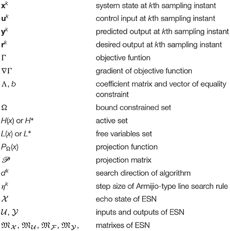
Symbols of the Model and Algorithm
Keywords: rehabilitation robot, model predictive control, intention recognition, conjugate gradient approach, projected operator
Citation: Shi T, Tian Y, Sun Z, Zhang B, Pang Z, Yu J and Zhang X (2020) A New Projected Active Set Conjugate Gradient Approach for Taylor-Type Model Predictive Control: Application to Lower Limb Rehabilitation Robots With Passive and Active Rehabilitation. Front. Neurorobot. 14:559048. doi: 10.3389/fnbot.2020.559048
Received: 05 May 2020; Accepted: 29 October 2020;
Published: 03 December 2020.
Edited by:
Poramate Manoonpong, University of Southern Denmark, DenmarkReviewed by:
Hong Zeng, Southeast University, ChinaCopyright © 2020 Shi, Tian, Sun, Zhang, Pang, Yu and Zhang. This is an open-access article distributed under the terms of the Creative Commons Attribution License (CC BY). The use, distribution or reproduction in other forums is permitted, provided the original author(s) and the copyright owner(s) are credited and that the original publication in this journal is cited, in accordance with accepted academic practice. No use, distribution or reproduction is permitted which does not comply with these terms.
*Correspondence: Zhongbo Sun, emJzdW5AY2N1dC5lZHUuY24=; Junzhi Yu, eXVqdW56aGlAcGt1LmVkdS5jbg==
Disclaimer: All claims expressed in this article are solely those of the authors and do not necessarily represent those of their affiliated organizations, or those of the publisher, the editors and the reviewers. Any product that may be evaluated in this article or claim that may be made by its manufacturer is not guaranteed or endorsed by the publisher.
Research integrity at Frontiers
Learn more about the work of our research integrity team to safeguard the quality of each article we publish.