Choose your tools carefully: a comparative evaluation of deterministic vs. stochastic and binary vs. analog neuron models for implementing emerging computing paradigms

Neuromorphic computing, commonly understood as a computing approach built upon neurons, synapses, and their dynamics, as opposed to Boolean gates, is gaining large mindshare due to its direct application in solving current and future computing technological problems, such as smart sensing, smart devices, self-hosted and self-contained devices, artificial intelligence (AI) applications, etc. In a largely software-defined implementation of neuromorphic computing, it is possible to throw enormous computational power or optimize models and networks depending on the specific nature of the computational tasks. However, a hardware-based approach needs the identification of well-suited neuronal and synaptic models to obtain high functional and energy efficiency, which is a prime concern in size, weight, and power (SWaP) constrained environments. In this work, we perform a study on the characteristics of hardware neuron models (namely, inference errors, generalizability and robustness, practical implementability, and memory capacity) that have been proposed and demonstrated using a plethora of emerging nano-materials technology-based physical devices, to quantify the performance of such neurons on certain classes of problems that are of great importance in real-time signal processing like tasks in the context of reservoir computing. We find that the answer on which neuron to use for what applications depends on the particulars of the application requirements and constraints themselves, i.e., we need not only a hammer but all sorts of tools in our tool chest for high efficiency and quality neuromorphic computing.

1 Introduction

High-performance computing has historically developed around the Boolean computing paradigm, executed on silicon (Si) complementary metal oxide semiconductor (CMOS) hardware. In fact, software has for decades been developed around the CMOS fabric that has singularly dictated our choice of materials, devices, circuits, and architecture–leading to the dominant processor design paradigm: von Neumann architecture that separates memory and processing units. Over the last decade, however, Moore’s law for hardware scaling has significantly slowed down, primarily due to the prohibitive energy cost of computing and an increasingly steep memory wall. At the same time, software development has significantly evolved around “Big Data” paradigm, with machine learning and artificial intelligence (AI) dominating the roost. Additionally, the push towards the internet of things (IoT) edge devices has prompted an intensive search for energy-efficient and compact hardware systems for on-chip data processing (Big data, 2018).

One such direction is neuromorphic computing, which uses the concept of mimicking a human brain architecture to design circuits and systems that can perform highly energy-efficient computations (Mead, 1990; Schuman et al., 2017; Marković et al., 2020; Christensen et al., 2022; Kireev et al., 2022). A human brain is primarily composed of two functional elemental units - synapses and neurons. Neurons are interconnected through synapses with different connection strengths (commonly known as synaptic weights), which provide the learning and memory capabilities of the brain. A neuron receives synaptic inputs from other neurons, generates output in the form of action potentials, and distributes the output to the subsequent neurons. A human brain has $\sim 10^{11}$ neurons and $\sim 10^{15}$ synapses and consumes $\sim 1-10$ f J per synaptic event (Kandel et al., 2000; Squire et al., 2012; Upadhyay et al., 2016).

To emulate the organization and functionality of a human brain, there are many proposals for physical neuromorphic computing systems using memristors (Yao et al., 2020; Duan et al., 2020; Moon et al., 2019), spintronics (Grollier et al., 2020; Locatelli et al., 2014; Lv et al., 2022), charge-density-wave (CDW) devices (Liu et al., 2021), photonics (Shastri et al., 2021; Shainline et al., 2017), etc. In recent years, there has been significant progress in the development of physical neuromorphic hardware, both in academia and industry. The hierarchy of neuromorphic hardware implementation spans from the system level to the device level and all the way down to the level of the material. At the system level, various large-scale neuromorphic computers utilize different approaches - for instance, IBM’s TrueNorth (Merolla et al., 2014), Intel’s Loihi (Davies et al., 2018), SpiNNaker (Furber et al., 2014), BrainScaleS (Schemmel et al., 2010), Tianjic chip (Pei et al., 2019), Neurogrid (Benjamin et al., 2014), etc. They support a broad class of problems ranging from complex to more general computations. At the device level, the most commonly used component is the memristor which can be utilized in synapse and neuron implementations (Jo et al., 2010; Serb et al., 2020; Innocenti et al., 2021; Mehonic and Kenyon, 2016). Memristor crossbars are frequently used to represent synapses in neuromorphic systems (Adam et al., 2016; Hu et al., 2014). Memristor can also provide stochasticity in the neuron model (Suri et al., 2015). Another emerging class of devices for neuromorphic computing is spintronics devices (Grollier et al., 2020). Spintronics devices can be implemented with low energy and high density and are compatible with existing CMOS technology (Sengupta et al., 2016a). The spintronics devices utilized in neuromorphic computing include spin-torque devices (Torrejon et al., 2017; Roy et al., 2014; Sengupta et al., 2016b), magnetic domain walls (Siddiqui et al., 2020; Leonard et al., 2022; Brigner et al., 2022), and skyrmions (Jadaun et al., 2022; Song et al., 2020). Optical or photonics devices are also implemented for neurons and synapses in recent years (Shastri et al., 2021; Romeira et al., 2016; Guo et al., 2021). The field is very new and many novel forms of neuron and synaptic devices can be designed to match the mathematical model of neural networks (NNs). Physical neuromorphic computing can implement these functionalities directly in their physical characteristics (I-I, V-V, I-V), which results in highly compact devices that are well-suited for scalable and energy-efficient neuromorphic systems (Camsari et al., 2017a; Camsari et al., 2017b; Ganguly et al., 2021; Yang et al., 2013). This is critical as current NN-based computing is highly centralized (resident-on and accessed-via cloud) and is energy inefficient because the underlying volatile, often von Neumann, digital Boolean-based system design unit has to emulate inherently analog, mostly non-volatile distributed computing model of neural systems, even if at a simple abstraction level (Merolla et al., 2014). Recent advances in custom design such as FPGAs (Wang et al., 2018) and more experimental Si FPNAs (Farquhar et al., 2006) have demonstrated that a new form of device design rather than emulation is the way to go, and physical neuromorphic computing based on emerging technology can go a long way to achieve this (Rajendran and Alibart, 2016).

There is an increased use of noise-as-a-feature rather than a nuisance in NN models (Faisal et al., 2008; Baldassi et al., 2018; Goldberger and Ben-Reuven, 2017), and physical neuromorphic computing can provide natural stochasticity, with various noise colors depending on the device physics (Vincent et al., 2015; Brown et al., 2019). Some prominent areas where stochasticity and noise have been used include training generalizability (Jim et al., 1996), stochastic sampling (Cook, 1986), and recently proposed and coming into prominence, diffusion-based generative models (Huang et al., 2021). In all these models, noise plays a fundamental role, i.e., these algorithms do not work without inherent noise.

It is therefore critical to study and analyze the kinds of devices that will be useful to implement physical neuromorphic computing. We understand from neurobiology that there is a large degree of neuron design customization that has developed through evolution to obtain high task-based performance. Similarly, a variety of mathematical models of neurons have been designed in NN literature as well (Schuman et al., 2017; Burkitt, 2006; Ganguly et al., 2021). It is quite likely that the area of physical neuromorphics will use a variety of device designs rather than the uniformity of NAND gate-based design commonly seen in Boolean-based design, to achieve the true benefits of energy efficiency and scalability brought forth by this paradigm of system design.

In this work, we study a subset of this wide variety of neuron designs that are well-represented and easily available from many proposed physical neuromorphic platforms to understand and analyze their task specialization. In particular, we analyze analog and binary neuron models, including stochasticity in the model, for analog temporal inferencing tasks, and evaluate and compare their performances. We numerically estimate the performance metric normalized means squared error (NMSE), discuss the effect of stochasticity on prediction accuracy vs. robustness, and show the hardware implementability of the models. Furthermore, we estimate the memory capacity for different neuron models. Our results suggest that analog stochastic neurons perform better for analog temporal inferencing tasks both in terms of prediction accuracy and hardware implementability. Additionally, analog neurons show larger memory capacity. Our findings may provide a potential path forward toward efficient neuromorphic computing.

2 Brief overview on neuron models

An essential function of a neuron in a NN is processing the weighted synaptic inputs and generating an output response. A single biological neuron itself is a complex dynamical system (Bick et al., 2020). Proposed artificial neurons in most implementations of NNs (either software or hardware) are significantly simpler unless they specifically attempt to mimic the biological neuron (Harmon, 1959; Schuman et al., 2017; 2022). As such their mathematical representations are cheaper and a significant amount of computational capabilities derive from the network itself. However, a NN is an interplay of the neurons, the synapses, and the network structure itself, and therefore the neuron model itself may provide certain capabilities that can help make a more efficient NN, in the context of the application specialization (Abiodun et al., 2018).

The set of behavior over which such neurons can be classified and analyzed is vast and may include spiking vs. non-spiking behavior with associated data representation, deterministic vs. stochastic output response function, discrete (or binary) vs. continuous (or analog) output response function, the particular mathematical model of the output response function itself (e.g., sigmoid, tanh, ReLU), presence or absence of memory states with a neuron, etc (Goodfellow et al., 2016; Davidson and Furber, 2021; Barna and Kaski, 1990). In the software NN world, specialization of certain neural models and connectivity are well appreciated, as an example sparse vs. dense vs. convolutional layers, or the use of ReLU neurons in the hidden layers vs. sigmoidal, softmax layers at outputs employed in many computer vision tasks (Szandała, 2020; Zhang and Woodland, 2015; Oostwal et al., 2021). Figure 1A schematically shows the output characteristics of different types of widely used neuron models.

FIGURE 1

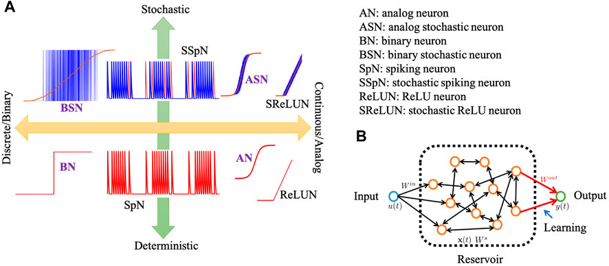
FIGURE 1. (A) Schematic of different types of widely used neuron models with their output characteristics. In the bottom panel, all the red curves represent the deterministic neurons’ output characteristics. In the top panel, the blue curves represent the actual stochastic output characteristics while the red is the corresponding deterministic/expected value of the output $(<stochasticoutput>)$ characteristics. Spiking neurons (SpN and SSpN) can be considered in between the two limits of purely binary vs. purely analog neurons. Please note that we only analyze the analog and binary neurons (including their stochastic counterparts) in this work, as indicated by the purple-colored bold font labels. (B) Schematic of a reservoir setup using neurons connected with each other bidirectionally with random weights.

In this work, we have focused on two particular behaviors of neural models that we believe can capture a significant application space, particularly in the domain of lightweight real-time signal processing tasks, and are readily built from emerging materials technology. We specifically look at binary vs. analog and deterministic vs. stochastic neuron output response functions (purple-colored bold font labels in Figure 1A). We also use them in a reservoir computing (RC)-like context for signal processing tasks for our analysis. Reservoir computing uses the dynamics of a recurrently connected network of neurons to project an input (spatio-)temporal signal onto a high dimensional phase space, which forms the basis of inference, typically via a shallow 1-layer linear transform or a multi-layer feedforward network (Tanaka et al., 2019; Triefenbach et al., 2010; Jalalvand et al., 2015; Ganguly et al., 2018; Moon et al., 2019). A schematic of a reservoir is shown in Figure 1B where the neurons are connected with each other bidirectionally with random weights. Multiple reservoirs may be connected hierarchically for more complex deep RC architecture. RC may be considered as a machine learning analog of an extended Kalman filter where the state space and the observation models are learned and not designed a priori (Tanaka et al., 2019).

Our choice of evaluating these specific behavior differences on an RC-based NN reflects the prominent use-case that is made out for many emerging nano-materials technology-based neuron and synaptic devices, viz. energy-efficient learning, and inference at the edge. These tasks often end up involving temporal or spatio-temporal data processing to extract relevant and actionable information, some examples being anomaly detection (Kato et al., 2022), feature tracking (Abreu Araujo et al., 2020), optimal control (Engedy and Horváth, 2012), and event prediction (Pyragas and Pyragas, 2020), all of which are well-suited for an RC-based NN. Therefore this testbench forms a great intersection for our analysis.

It should be noted that we do not include spiking neurons in this particular analysis. Spiking neurons have significantly different data encoding (level vs. rate or inter-spike interval encoding) and learning mechanisms (back-propagation or regression vs. spike-time dependent plasticity) that it is hard to disentangle the neuron model itself from demonstrated tasks, therefore we leave such a contrasting analysis of spiking neuron devices with non-spiking variants for a future study.

The neurons are modeled in the following way:

$\mathbf{y}=f_N\left(\sum w^T\mathbf{x}\right)+r_N(1)$

Here the symbols have the usual meaning, i.e., y is the output activation of the neuron, f_N is the activation function, which is a sigmoidal or hyperbolic tangent for most non-spiking hardware neurons, and r_N is a random sample drawn from a random uniform distribution to represent stochasticity. It is possible to use a ReLU-like activation function or some other distribution for sampling stochasticity, particularly if the hardware neuron shows colored noise behavior, we do not particularize for such details and keep the analysis confined to the most common hardware neuron variants. Therefore, in our analysis, the r_N term is weighed down by an arbitrary factor to mimic the degree of stochasticity displayed by the neuron, and the f_N is either a continuous tanh() for analog neuron or a sgn(tanh()) for a binary neuron (sgn() being the signum function).

3 Methods

As discussed previously, the neuron models are analyzed in the context of a reservoir computer, specifically an echo-state network (ESN). An ESN is composed of a collection of recurrently connected neurons, with randomly distributed weights of the interconnects within this collection (Lukoševičius, 2012; Li et al., 2012). This forms the “reservoir”, which is activated by an incoming signal, and whose output is read by an output layer trained via linear regression.

We employ different neuron models in this work, such as analog and binary neurons (with and without stochasticity in the model), which makes a total of four models at our disposal, namely, analog neuron (AN), analog stochastic neuron (ASN), binary neuron (BN), and binary stochastic neuron (BSN). The dynamical equations of the reservoirs built using different neuron models are described as follows (Ganguly et al., 2021):

$\begin{array}{cc}\hfill \text{AN}:\mathbf{x}\left[t+1\right]& =\left(1-a\right)*\mathbf{x}\left[t\right]+a*\mathit{tanh}\left(\mathbf{z}\left[t+1\right]\right)\hfill \\ \hfill \text{ASN}:\mathbf{x}\left[t+1\right]& =\left(1-a\right)*\mathbf{x}\left[t\right]+a*\mathit{tanh}\left(\mathbf{z}\left[t+1\right]\right)+b*r_N\left[t\right]\hfill \\ \hfill \text{BN}:\mathbf{x}\left[t+1\right]& =\left(1-a\right)*\mathbf{x}\left[t\right]+\mathit{sgn}\left(a*\mathit{tanh}\left(\mathbf{z}\left[t+1\right]\right)\right)\hfill \\ \hfill \text{BSN}:\mathbf{x}\left[t+1\right]& =\left(1-a\right)*\mathbf{x}\left[t\right]+\mathit{sgn}\left(a*\mathit{tanh}\left(\mathbf{z}\left[t+1\right]\right)+b*r_N\left[t\right]\right)\hfill \end{array}(2)$

where z[t + 1] = Wⁱⁿu[t + 1] + W^sx[t]. Here, u is the input vector, x[t] represents the reservoir state vector at the time t, a is the reservoir leaking rate (assumed to be the constant for all the neurons), b is the neuron noise scaling parameter to include stochasticity in the neuron model, r_N is a uniform random distribution, and Wⁱⁿ and W^s are the random weight matrices of input-reservoir and reservoir-reservoir connections, respectively. We use the same leaking rate across all models to ensure a fair comparison among the neuron models on an equal footing. It can be challenging to compare models that have different parameters as it can introduce biases. One of the unique features of reservoir computing is having random weight matrices (Tanaka et al., 2019) and we consider five different network topologies by creating five sets of W^s using random “seed” for various reservoir sizes, which makes our analysis unbiased to any particular network topology. The W^s elements are normalized using the spectral radius. We perform 1,000 simulations within each network topology making the total sample size 5,000 for every reservoir size within each neuron model. The output vector y is obtained as:

$\mathbf{y}=W^{\mathit{out}}\mathbf{x}(3)$

where W^out represents the reservoir-output weight matrix. We consider two different types of training methods, i.e., “offline” and “online” training. In the case of “offline” training, we extract the output weight matrix, W^out once at the end of the training cycle and use that static W^out for the testing cycle. In contrast, for “online” training, W^out is periodically updated throughout the testing cycle. The entire testing cycle is divided into 40 segments. The first segment uses the W^out extracted from the initial training cycle. We calculate a new W^out after the first segment of the testing cycle. Then, we update the W^out such that the elements are composed of 90% from the older version and 10% from the new one. The updated W^out is used for the second segment and the procedure keeps going on throughout the testing cycle. This stabilizes the learning at the cost of higher error rates as the learning evolution slowly evolves to a new configuration. This is akin to the successive over-relaxation methods used in many self-consistent numerical algorithms for improved convergence.

4 Results and discussions

4.1 Binary vs. analog: inference errors

We implement the temporal inferencing task, specifically, the time-series prediction task to test and compare the performance of different neuron models. We consider an input signal of the form u(t) = A cos(2πf₁t) + B sin(2πf₂t), which we referred to as a clean input. We use A = 1, B = 2, f₁ = 0.10 Hz, and f₂ = 0.02 Hz. Although we choose the magnitude and frequency of the input arbitrarily, we further investigate other combinations of these variables (Table 1) to ensure that our analysis remains independent of them. We train the neuron models using the clean input signal and test the models on a test signal from the same generator. The neuron models learn to reproduce the test signal from its previously self-generated output. The performance of the neuron models for time-series prediction tasks is usually measured by the NMSE, which is the metric that indicates how accurately the models can predict the test signal. If y_tar is the target output and y_pre is the actual predicted output, for N_T time steps, we define NMSE as:

$NMSE=\frac{1}{N_T\left(y_{\mathit{tar}}^{\mathit{max}}-y_{\mathit{tar}}^{\mathit{min}}\right)}{\displaystyle \sum _{i=1}^{i=N_T}}{\left(y_{\mathit{tar}}\left(i\right)-y_{\mathit{pre}}\left(i\right)\right)}^2(4)$

TABLE 1

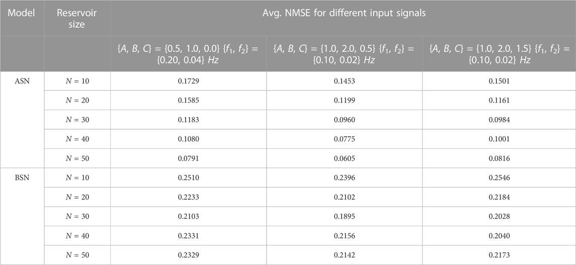
TABLE 1. Average NMSE data extracted from the ASN and BSN models (b = 5%) for various reservoir sizes. The form of the input signal is, u(t) = A cos(2πf₁t) + B sin(2πf₂t) + C[rand(1, t) − 0.5].

Figures 2A,B show the NMSE for ASN and BSN, respectively for the time-series prediction task for various reservoir sizes. We generate the results using the ‘offline’ training as discussed in the method section, for a clean input signal. We incorporate the stochasticity by adding 5% white noise in both neuron models (b = 0.05). The total sample size is 5,000 for a specific reservoir size, however, it is worth mentioning that we do not get valid NMSE for all the 5,000 cases because the network fails to predict the input signal and blows up for some cases. We get $\sim 90\%-100\%$ successful cases depending on the reservoir sizes. Only valid data points are included in Figure 2 and all the subsequent figures. We find ASN performs better than BSN for all the reservoir sizes indicated by the average NMSE (cyan dashed-dotted line). Overall the NMSE is less scattered for ASN than BSN, so is their standard deviation, (magenta dashed-dotted line) as shown in the bottom panel of Figure 2. For ASN, we find that the average NMSE has a decreasing trend as the reservoir size increases, which indicates larger size networks can predict better. This happens because of the substantially richer dynamics and phase-space volume possible in a large network. In contrast, for BSN, the average NMSE is almost unchanged as the reservoir size increases.

FIGURE 2

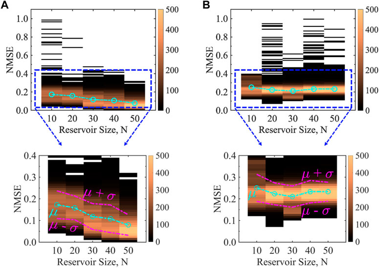
FIGURE 2. Comparison of NMSE for an analog time-series prediction task between (A) ASN and (B) BSN models as a function of reservoir size with 5% stochasticity incorporated in both the neuron models for a clean input signal. The form of the clean input signal is u(t) = A cos(2πf₁t) + B sin(2πf₂t), where A = 1, B = 2, f₁ = 0.10 Hz, and f₂ = 0.02 Hz. ASN performs better than BSN for the entire range of reservoir size as indicated by the average (μ) NMSE (cyan dashed-dotted line). ASN shows a decreasing trend in NMSE as a function of reservoir size while BSN results remain almost unchanged. The NMSE data for every reservoir size is obtained from five different reservoir topologies and 1,000 simulation runs (different random “seed”) within each topology (total sample size is 5,000). The color bar represents the frequency of the NMSE data. Note that in some cases, our model fails to generate a meaningful NMSE as the reservoir output blows up. We get meaningful output from $\sim 90\%-100\%$ cases depending on the reservoir sizes, and those data are plotted here and used to estimate the average NMSE. The bottom panel is the zoomed version of the top panel and the magenta dashed-dotted lines are the guide to the eye that shows the data distribution in the range of μ ± σ. The color codes to represent the μ and σ are the same for the subsequent figures henceforth.

We vary the stochasticity incorporated in the neuron models. Figures 3A,B show the distribution of the NMSE for different percentages of stochasticity, b for ASN and BSN models, respectively. We find that ASN performs better than its BSN counterpart throughout the ranges of b as indicated by the average NMSE. For ASN, the average NMSE shows a sub-linear trend as a function of b (Figure 3C) for various reservoir sizes, while for BSN, the average NMSE remains unchanged (Figure 3D). For pure analog neuron (b = 0%), the NMSE is not much spread out, and also, for larger reservoir size, the average NMSE is smaller than the neuron model with stochasticity, however, having a neuron model with zero stochasticity is not practical. Moreover, stochasticity helps to make the system stable and reliable as discussed in the next section. Although the average NMSE increases with increasing b, we conjecture that b = 2–5% would be optimal.

FIGURE 3

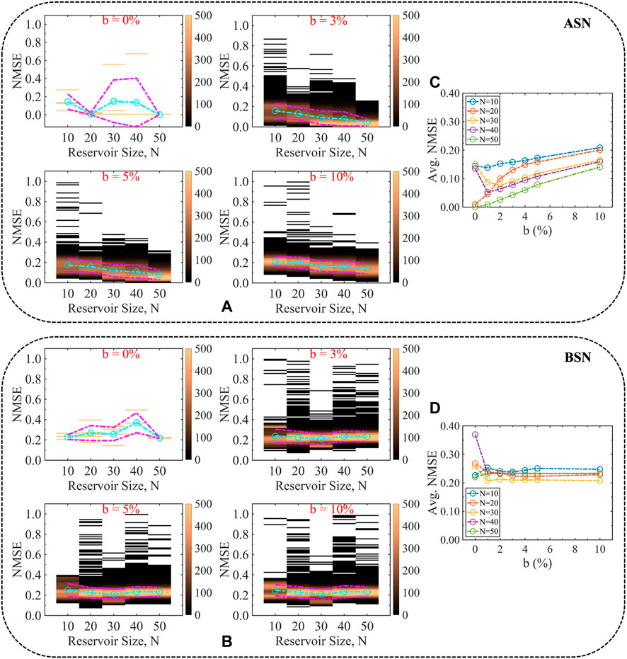
FIGURE 3. Evolution of NMSE for different degrees of stochasticity (noise percentages) associated with the (A) ASN and (B) BSN models. ASN performs better than the BSN model for analog time-series prediction tasks throughout the ranges of the degree of stochasticity as indicated by the average NMSE shown in (C) and (D) for ASN and BSN, respectively. The characteristics of the average NMSE as a function of reservoir size, i.e., the decreasing trend for ASN while almost no change for BSN holds throughout the range of b.

The aforementioned results are based on a clean input signal. We tested the models for distorted input as well. For the distorted case, we add a white noise in the clean input and the form of the distorted input signal is u(t) = A cos(2πf₁t) + B sin(2πf₂t) + C[rand(1, t) − 0.5]. The white noise is uniformly distributed for all t values, both in the positive and negative half of the sinusoidal input. The degree of noise has been chosen arbitrarily. Again, we show various degrees of noise (Table 1) to make the analysis independent of a specific value of the noise margin. The NMSE results shown in Figures 4A,B are calculated using A = 1, B = 2, C = 1, f₁ = 0.10 Hz, and f₂ = 0.02 Hz. We find a better performance for ASN than that of BSN for the distorted input as well. It appears that for ASN, with a distorted input signal, the spectrum of NMSE is smaller, which reduces the standard deviation. The characteristics of the average NMSE are similar for the clean and distorted input for both ASN (Figure 4C) and BSN (Figure 4D) models. However, the average NMSE is slightly lower for the distorted input for both types of neuron models. Furthermore, we use different combinations of signal magnitude, frequency, and the weight of noise in the input signal. We list the average NMSE for various reservoir sizes in Table 1. Additionally, we explore other input functions beyond the simple sinusoidal input used in the aforementioned results. In particular, we use a sinusoidal with higher harmonic terms, a sawtooth input function, and a square input function. The used form of the functions are $u(t)=\frac{4}{\pi }{\sum }_{i=1}^{15}\frac{1}{n}\sin 2\pi n{f}_{1}t$ (odd n), u(t) = A sawtooth(2πf₁t) + B sawtooth(2πf₂t), u(t) = A square(2πf₁t) + B square(2πf₂t), respectively. In the case of sinusoidal with higher harmonic terms, we use the fundamental frequency f₁ = 0.10 Hz. For the sawtooth and square inputs, the magnitude and frequency remain the same as of the original sinusoidal clean input. The results are summarized in Figure 5, where the label Input 1, Input 2, Input 3, and Input 4 correspond to the sinusoidal clean input, sinusoidal with higher harmonic terms, sawtooth, and square input functions, respectively. Figure 5 shows that for all the different inputs, ANS performance is better than BSN in terms of NMSE. Comparing all the cases, we conjecture that ASN performs better than BSN for the temporal inferencing task.

FIGURE 4

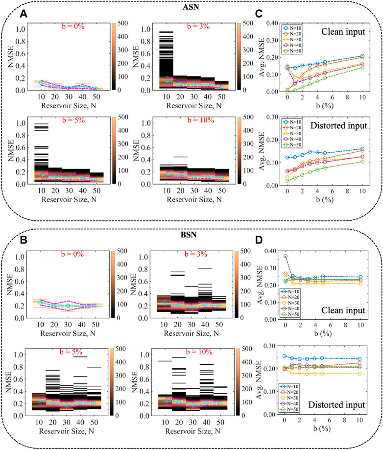
FIGURE 4. Evolution of NMSE for different degrees of stochasticity for (A) ASN and (B) BSN models for a distorted input signal. Random white noise is added to the clean input signal to introduce distortion and the form of the distorted signal is u(t) = A cos(2πf₁t) + B sin(2πf₂t) + C[rand(1, t) − 0.5], where A = 1, B = 2, C = 1, f₁ = 0.10 Hz, and f₂ = 0.02 Hz. ASN performs better than BSN for the distorted input, as indicated by the average NMSE shown in (C) and (D) for ASN and BSN, respectively, which dictates the robustness of the ASN model in terms of performance irrespective of the input signals.

FIGURE 5

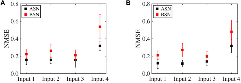
FIGURE 5. Comparison of NMSE for time-series prediction task between ASN and BSN models for various input functions for a reservoir size of (A) N = 20 and (B) N = 30. The degree of stochasticity incorporated in both neuron models is 5%. The label Input 1, Input 2, Input 3, and Input 4 correspond to the sinusoidal clean input, sinusoidal with higher harmonic terms, sawtooth, and square input functions, respectively. ANS performance is better than BSN in terms of NMSE for different input functions.

4.2 Deterministic vs. stochastic: generalizability and robustness

One important aspect of any NN implementation is the generalizability and robustness of the learning. A model trained to a very specific data distribution will fail when it is running on a distribution that differs from the trained model. This is particularly true if a generative model guides its own subsequent learning, which is the example we have used in our online learning scenario. In this case, the underlying distribution is varied slowly while the network evolves its internal generative model to match the output of distribution, i.e., it works as a dynamically evolving temporal auto-encoder.

The stochasticity of the neuron response will add errors to the generated output as we see in the previous cases, however, we find that after a few iterations of the online learning cycle, the ability of this online learning blows up, i.e., the linear regression-based learning cannot keep up with the test distribution evolution and the error builds up (we call it blowup) and the whole training needs to be fully reset or reinitiated and cannot merely evolve from previous learning. This blowup occurs 100% for deterministic analog neurons, and the rate reduces as the degree of stochasticity increases (parameter b).

This is shown in Table 2 for various input functions. It should be noted that at very high stochasticity while the training is more robust, the errors will be high, therefore a minimal amount of stochasticity is useful as a trade-off between these ends. The degree to which the trade-off can be performed depends on the application scenario. If full retraining is too expensive or not acceptable, then a relatively higher degree of stochasticity in the neuron is necessary, but if it is cheap and acceptable to retrain the whole network frequently, a near-deterministic neuron will be better suited to meet the requirements.

TABLE 2

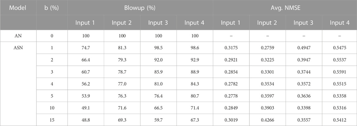
TABLE 2. Robustness vs. accuracy trade-off (N = 20). The label Input 1, Input 2, Input 3, and Input 4 correspond to the sinusoidal clean input, sinusoidal with higher harmonic terms, sawtooth, and square input functions described earlier, respectively.

4.3 Synaptic weights dynamic range: hardware implementability

One critical aspect of hardware implementability of neuromorphic computing is the ability to modulate the weights and the dynamic range or the order of magnitude to which weights may be distributed. It can be shown that a 30-bit weight resolution represents about a 100 dB dynamic range. While such ranges might be comparatively easily implemented in software, it is significantly difficult to implement such a high dynamic range in physical hardware. While some memristive materials may show multi-steps, it is hard to achieve much more than one order of magnitude change in the weights. Please note that we do not mean the change in the physical characteristics (typically the resistance) used to represent the weights themselves, but rather the number of steps that the weight can be implemented as.

We compare the dynamic range of the learned synaptic weights that need to be implemented in the reservoir networks (in the trained output readout layer) for various input functions and find that the ASN networks show the smallest dynamic range for all the cases (Figure 6) and suggest the easiest path to hardware implementability of physical neuromorphic computing. It is important to note that the hardware implementation of neuromorphic computing is an open question and the dynamic range of the synaptic weights is one of the important factors when it comes to the physical deployment of neuromorphic computing as discussed above. ASN networks show better performance in terms of the dynamic range of learned synaptic weights compared to other models, which suggests that networks that employed ASN models might have better hardware implementability; however, it requires more analysis in terms of energy cost, scalability, and reconfigurability, which we leave as a future study.

FIGURE 6

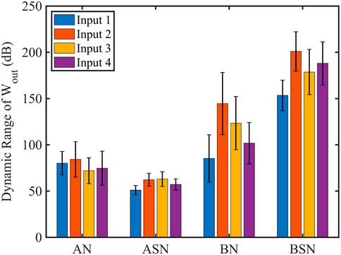
FIGURE 6. Dynamic range of the learned synaptic weights, W_out for all the neuron models (N =20). 5% stochasticity is considered in the ASN and BSN models. ASN model shows the smallest dynamic range that leads to better hardware implementability. The label Input 1, Input 2, Input 3, and Input 4 correspond to the sinusoidal clean input, sinusoidal with higher harmonic terms, sawtooth, and square input functions, respectively.

4.4 Memory capacity

The performance of reservoir computing is often described by memory capacity (MC) (Jaeger, 2002; Verstraeten et al., 2007; Inubushi and Yoshimura, 2017). It measures how much information from previous input is present in the current output state of the reservoir. The task is to reproduce the delayed version of the input signal. For a certain time delay k, we measure how well the current state of the reservoir y_k(t) can recall the input u at time t − k. The linear MC is defined as:

$MC={\displaystyle \sum _k}\frac{{cov}^2\left(u\left(t-k\right),y_k\left(t\right)\right)}{{\sigma }^{2}u\left(t-k\right){\sigma }^2\left(y_k\left(t\right)\right)}(5)$

where u(t − k) is the delayed version of the input signal, which is the target output, and y_k(t) is the output of the reservoir unit trained on the delay k. cov and σ² denote covariance and variance, respectively.

Table 3 shows the linear MC for different neuron models for the distorted input u(t) = A cos(2πf₁t) + B sin(2πf₂t) + C[rand(1, t) − 0.5], where A = 1, B = 2, C = 1, f₁ = 0.10 Hz, and f₂ = 0.02 Hz. We consider the delayed signal over 1 to 50 timesteps, meaning k spans from 1 to 50. We find that Analog neurons have significantly larger linear MC than binary neurons. For analog neurons, linear MC increases as the reservoir size increases, which is expected because a larger dynamical system can retain more information from the past (Jaeger, 2002). Additionally, including stochasticity in the analog neuron model degrades the linear MC as reported previously (Jaeger, 2002). In contrast, binary neurons fail to produce substantial differences in linear MC when reservoir size is varied and stochasticity is included in the model.

TABLE 3

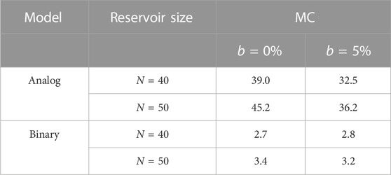
TABLE 3. Linear memory capacity (MC) for different neuron models.

Besides the previously mentioned properties, physical neuromorphic computing exhibits chaos or edge-of-chaos property, which has been shown to enhance the performance of complex learning tasks (Kumar et al., 2017; Hochstetter et al., 2021; Nishioka et al., 2022). The edge-of-chaos property refers to the transition point between ordered and chaotic behavior in a system. In the discussed models, it may be possible to achieve the edge-of-chaos state by introducing increasing amounts of noise to the models, resulting in chaotic behavior that could potentially improve network performance. We find that with an increased degree of stochasticity in the neuron models, the learning process becomes more robust, which could be a signature of the performance improvement by including the edge-of-chaos property. However, the prediction accuracy and the linear MC tend to decrease with a higher degree of stochasticity, so the trade-off needs to be considered. It should be noted that a more comprehensive analysis is required to fully understand the impact of edge-of-chaos behavior on the discussed neuron models, which is beyond the scope of this paper and will be explored in future studies.

5 Conclusion

In summary, we studied different neuron models for the analog signal inferencing (time-series prediction) task in the context of reservoir computing and evaluate their performances for various input functions. We show that the performance metrics are better for ASN than BSN for both clean and distorted input signals. We find that the increasing degree of stochasticity makes the models more robust, however, decreases the prediction accuracy. This introduces a trade-off between accuracy and robustness depending on the application requirements and specifications. Furthermore, the ASN model turns out to be the suitable one for hardware implementation, which attributes to the smallest dynamics range of the learned synaptic weights, although other aspects, i.e., energy requirement, scalability, and reconfigurability need to be assessed. Additionally, we estimate the linear memory capacity for different neuron models, which suggests that analog neurons have a higher ability to reconstruct the past input signal from the present reservoir state. These findings may provide critical insights for choosing suitable neuron models for real-time signal-processing tasks and pave the way toward building energy-efficient neuromorphic computing platforms.

Data availability statement

The raw data supporting the conclusions of this article will be made available by the authors, without undue reservation.

Author contributions

SG, MM, and AG conceived the idea. SG wrote the base simulation codes and MM modified and parallelized the base simulation codes for HPC, performed all the simulations, and generated the results. All authors analyzed the results, contributed to the manuscript, and approved the submitted version.

Funding

This work was supported by DRS Technology and in part by the NSF I/UCRC on Multi-functional Integrated System Technology (MIST) Center; IIP-1439644, IIP-1439680, IIP-1738752, IIP-1939009, IIP-1939050, and IIP-1939012.

Acknowledgments

We thank Kerem Yunus Camsari, Marco Lopez, Tony Ragucci, and Faiyaz Elahi Mullick for useful discussions. All the calculations are done using the computational resources from High-Performance Computing systems at the University of Virginia (Rivanna) and the Extreme Science and Engineering Discovery Environment (XSEDE).

Conflict of interest

The authors declare that the research was conducted in the absence of any commercial or financial relationships that could be construed as a potential conflict of interest.

Publisher’s note

All claims expressed in this article are solely those of the authors and do not necessarily represent those of their affiliated organizations, or those of the publisher, the editors and the reviewers. Any product that may be evaluated in this article, or claim that may be made by its manufacturer, is not guaranteed or endorsed by the publisher.

References

Abiodun, O. I., Jantan, A., Omolara, A. E., Dada, K. V., Mohamed, N. A., and Arshad, H. (2018). State-of-the-art in artificial neural network applications: A survey. Heliyon 4 (11), e00938. doi:10.1016/j.heliyon.2018.e00938

PubMed Abstract | CrossRef Full Text | Google Scholar

Abreu Araujo, F., Riou, M., Torrejon, J., Tsunegi, S., Querlioz, D., Yakushiji, K., et al. (2020). Role of non-linear data processing on speech recognition task in the framework of reservoir computing. Sci. Rep. 10, 1–11. doi:10.1038/s41598-019-56991-x

PubMed Abstract | CrossRef Full Text | Google Scholar

Adam, G. C., Hoskins, B. D., Prezioso, M., Merrikh-Bayat, F., Chakrabarti, B., and Strukov, D. B. (2016). 3-D memristor crossbars for analog and neuromorphic computing applications. IEEE Trans. Electron Devices 64 (1), 312–318. doi:10.1109/TED.2016.2630925

CrossRef Full Text | Google Scholar

Baldassi, C., Gerace, F., Kappen, H. J., Lucibello, C., Saglietti, L., Tartaglione, E., et al. (2018). Role of synaptic stochasticity in training low-precision neural networks. Phys. Rev. Lett. 120 (26), 268103. doi:10.1103/PhysRevLett.120.268103

PubMed Abstract | CrossRef Full Text | Google Scholar

Barna, G., and Kaski, K. (1990). Stochastic vs. Deterministic neural networks for pattern recognition. Phys. Scr. T33, 110–115. doi:10.1088/0031-8949/1990/T33/019

CrossRef Full Text | Google Scholar

Benjamin, B. V., Gao, P., McQuinn, E., Choudhary, S., Chandrasekaran, A. R., Bussat, J. M., et al. (2014). Neurogrid: A mixed-analog-digital multichip system for large-scale neural simulations. Proc. IEEE 102 (5), 699–716. doi:10.1109/JPROC.2014.2313565

CrossRef Full Text | Google Scholar

Bick, C., Goodfellow, M., Laing, C. R., and Martens, E. A. (2020). Understanding the dynamics of biological and neural oscillator networks through exact mean-field reductions: A review. J. Math. Neurosci. 10 (1), 9–43. doi:10.1186/s13408-020-00086-9

PubMed Abstract | CrossRef Full Text | Google Scholar

Big data (2018). Big data needs a hardware revolution. Nature 554, 145–146. doi:10.1038/d41586-018-01683-1

PubMed Abstract | CrossRef Full Text | Google Scholar

Brigner, W. H., Hassan, N., Hu, X., Bennett, C. H., Garcia-Sanchez, F., Cui, C., et al. (2022). Domain wall leaky integrate-and-fire neurons with shape-based configurable activation functions. IEEE Trans. Electron Devices 69 (5), 2353–2359. doi:10.1109/TED.2022.3159508

CrossRef Full Text | Google Scholar

Brown, S. D., Chakma, G., Musabbir Adnan, M, Hasan Sakib, M, and Rose, G. S. (2019). “Stochasticity in neuromorphic computing: Evaluating randomness for improved performance,” in 2019 26th IEEE International Conference on Electronics, Circuits and Systems (ICECS), Genoa, Italy, 27-29 November 2019 (IEEE), 454–457. doi:10.1109/ICECS46596.2019.8965057

CrossRef Full Text | Google Scholar

Burkitt, A. N. (2006). A review of the integrate-and-fire neuron model: I. Homogeneous synaptic input. Biol. Cybern. 95 (1), 1–19. doi:10.1007/s00422-006-0068-6

PubMed Abstract | CrossRef Full Text | Google Scholar

Camsari, K. Y., Faria, R., Sutton, B. M., and Datta, S. (2017a). Stochastic p-bits for invertible logic. Phys. Rev. X 7 (3), 031014. doi:10.1103/PhysRevX.7.031014

CrossRef Full Text | Google Scholar

Camsari, K. Y., Salahuddin, S., and Datta, S. (2017b). Implementing p-bits with embedded MTJ. IEEE Electron Device Lett. 38 (12), 1767–1770. ISSN 1558-0563. doi:10.1109/LED.2017.2768321

CrossRef Full Text | Google Scholar

Christensen, D. V., Dittmann, R., Linares-Barranco, B., Sebastian, A., Gallo, M. L., Redaelli, A., et al. (2022). 2022 roadmap on neuromorphic computing and engineering. Neuromorph. Comput. Eng. 2 (2), 022501. doi:10.1088/2634-4386/ac4a83

CrossRef Full Text | Google Scholar

Cook, R. L. (1986). Stochastic sampling in computer graphics. ACM Trans. Graph. 5 (1), 51–72. doi:10.1145/7529.8927

CrossRef Full Text | Google Scholar

Davidson, S., and Furber, S. B. (2021). Comparison of artificial and spiking neural networks on digital hardware. Front. Neurosci. 15, 651141. doi:10.3389/fnins.2021.651141

PubMed Abstract | CrossRef Full Text | Google Scholar

Davies, M., Srinivasa, N., Lin, T. H., Chinya, G., Cao, Y., Choday, S. H., et al. (2018). Loihi: A neuromorphic manycore processor with on-chip learning. IEEE Micro 38 (1), 82–99. doi:10.1109/MM.2018.112130359

CrossRef Full Text | Google Scholar

Duan, Q., Jing, Z., Zou, X., Wang, Y., Yang, K., Zhang, T., et al. (2020). Spiking neurons with spatiotemporal dynamics and gain modulation for monolithically integrated memristive neural networks. Nat. Commun. 11, 3399. doi:10.1038/s41467-020-17215-3

PubMed Abstract | CrossRef Full Text | Google Scholar

Engedy, István, and Horváth, Gábor (2012). “Optimal control with reinforcement learning using reservoir computing and Gaussian mixture,” in 2012 IEEE International Instrumentation and Measurement Technology Conference Proceedings, Graz, Austria, 13-16 May 2012 (IEEE), 1062–1066.

CrossRef Full Text | Google Scholar

Faisal, A., Selen, L. P. J., and Wolpert, D. M. (2008). Noise in the nervous system. Nat. Rev. Neurosci. 9 (4), 292–303. doi:10.1038/nrn2258

PubMed Abstract | CrossRef Full Text | Google Scholar

Farquhar, E., Gordon, C., and Hasler, P. (2006). “A field programmable neural array,” in 2006 IEEE International Symposium on Circuits and Systems, Kos, Greece, 21-24 May 2006 (IEEE). doi:10.1109/ISCAS.2006.1693534

CrossRef Full Text | Google Scholar

Furber, S. B., Galluppi, F., Temple, S., and Plana, L. A. (2014). The SpiNNaker project. Proc. IEEE 102 (5), 652–665. doi:10.1109/JPROC.2014.2304638

CrossRef Full Text | Google Scholar

Ganguly, S., Camsari, K. Y., and Ghosh, A. W. (2021). Analog signal processing using stochastic magnets. IEEE Access 9, 92640–92650. doi:10.1109/ACCESS.2021.3075839

CrossRef Full Text | Google Scholar

Ganguly, S., Gu, Y., Stan, M. R., and Ghosh, A. W. (2018). “Hardware based spatio-temporal neural processing backend for imaging sensors: Towards a smart camera,” in Image sensing technologies: Materials, devices, systems, and applications V (Washington USA: SPIE), 135–145. doi:10.1117/12.2305137

CrossRef Full Text | Google Scholar

Goldberger, J., and Ben-Reuven, E. (2017). “Training deep neural-networks using a noise adaptation layer,” in International Conference on Learning Representations, Toulon, France, April 24 - 26, 2017.

Google Scholar

Goodfellow, I., Bengio, Y., and Courville, A. (2016). Deep learning. Massachusetts, US: MIT press.

Google Scholar

Grollier, J., Querlioz, D., Camsari, K. Y., Everschor-Sitte, K., Fukami, S., and Stiles, M. D. (2020). Neuromorphic spintronics. Nat. Electron. 3 (7), 360–370. doi:10.1038/s41928-019-0360-9

CrossRef Full Text | Google Scholar

Guo, X., Xiang, J., Zhang, Y., and Su, Y. (2021). Integrated neuromorphic photonics: Synapses, neurons, and neural networks. Adv. Photonics Res. 2 (6), 2000212. doi:10.1002/adpr.202000212

CrossRef Full Text | Google Scholar

Harmon, L. D. (1959). Artificial neuron. Science 129 (3354), 962–963. doi:10.1126/science.129.3354.962

PubMed Abstract | CrossRef Full Text | Google Scholar

Hochstetter, J., Zhu, R., Loeffler, A., Diaz-Alvarez, A., Nakayama, T., and Kuncic, Z. (2021). Avalanches and edge-of-chaos learning in neuromorphic nanowire networks. Nat. Commun. 12 (4008), 4008–4013. doi:10.1038/s41467-021-24260-z

PubMed Abstract | CrossRef Full Text | Google Scholar

Hu, M., Li, H., Chen, Y., Wu, Q., Rose, G. S., and Linderman, R. W. (2014). Memristor crossbar-based neuromorphic computing system: A case study. IEEE Trans. Neural Netw. Learn. Syst. 25 (10), 1864–1878. doi:10.1109/TNNLS.2013.2296777

PubMed Abstract | CrossRef Full Text | Google Scholar

Huang, C. W., Lim, J. H., and Courville, A. C. (2021). A variational perspective on diffusion-based generative models and score matching. Adv. Neural Inf. Process. Syst. 34, 22863–22876.

Google Scholar

Innocenti, G., Di Marco, M., Tesi, A., and Forti, M. (2021). Memristor circuits for simulating neuron spiking and burst phenomena. Front. Neurosci. 15, 681035. doi:10.3389/fnins.2021.681035

PubMed Abstract | CrossRef Full Text | Google Scholar

Inubushi, M., and Yoshimura, K. (2017). Reservoir computing beyond memory-nonlinearity trade-off. Sci. Rep. 7, 1–10. doi:10.1038/s41598-017-10257-6

PubMed Abstract | CrossRef Full Text | Google Scholar

Jadaun, P., Cui, C., Liu, S., and Incorvia, J. A. C. (2022). Adaptive cognition implemented with a context-aware and flexible neuron for next-generation artificial intelligence. PNAS Nexus 1 (5), pgac206. doi:10.1093/pnasnexus/pgac206

PubMed Abstract | CrossRef Full Text | Google Scholar

Jaeger, H. (2002). Short term memory in echo state networks. gmd-report 152. Sankt Augustin: GMD-German National Research Institute for Computer Science.

Google Scholar

Jalalvand, A., Van Wallendael, G, and Walle, R. V. D (2015). “Real-time reservoir computing network-based systems for detection tasks on visual contents,” in 2015 7th International Conference on Computational Intelligence, Communication Systems and Networks, Riga, Latvia, 03-05 June 2015 (IEEE), 146–151. doi:10.1109/CICSyN.2015.35

CrossRef Full Text | Google Scholar

Jim, K. C., Giles, C. L., and Horne, B. G. (1996). An analysis of noise in recurrent neural networks: Convergence and generalization. IEEE Trans. Neural Netw. 7 (6), 1424–1438. doi:10.1109/72.548170

PubMed Abstract | CrossRef Full Text | Google Scholar

Jo, S. H., Chang, T., Ebong, I., Bhadviya, B. B., Mazumder, P., and Lu, W. (2010). Nanoscale memristor device as synapse in neuromorphic systems. Nano Lett. 10 (4), 1297–1301. doi:10.1021/nl904092h

PubMed Abstract | CrossRef Full Text | Google Scholar

Kandel, E. R., Schwartz, J. H., Jessell, T. M., Siegelbaum, S., Hudspeth, A. J., Mack, S., et al. (2000). Principles of neural science. New York: McGraw-Hill.

Google Scholar

Kato, J., Tanaka, G., Nakane, R., and Hirose, A. (2022). “Proposal of reconstructive reservoir computing to detect anomaly in time-series signals,” in 2022 International Joint Conference on Neural Networks (IJCNN), Padua, Italy, 18-23 July 2022 (IEEE), 1–6. doi:10.1109/IJCNN55064.2022.9892805

CrossRef Full Text | Google Scholar

Kireev, D., Liu, S., Jin, H., Patrick Xiao, T., Bennett, C. H., Akinwande, D., et al. (2022). Metaplastic and energy-efficient biocompatible graphene artificial synaptic transistors for enhanced accuracy neuromorphic computing. Nat. Commun. 13, 4386. doi:10.1038/s41467-022-32078-6

PubMed Abstract | CrossRef Full Text | Google Scholar

Kumar, S., Strachan, J. P., and Stanley Williams, R. (2017). Chaotic dynamics in nanoscale NbO2 Mott memristors for analogue computing. Nature 548 (7667), 318–321. doi:10.1038/nature23307

PubMed Abstract | CrossRef Full Text | Google Scholar

Leonard, T., Liu, S., Alamdar, M., Jin, H., Cui, C., Akinola, O. G., et al. (2022). Shape-dependent multi-weight magnetic artificial synapses for neuromorphic computing. Adv. Electron. Mat. 8 (12), 2200563. doi:10.1002/aelm.202200563

CrossRef Full Text | Google Scholar

Li, D., Han, M., and Wang, J. (2012). Chaotic time series prediction based on a novel robust echo state network. IEEE Trans. Neural Netw. Learn. Syst. 23 (5), 787–799. doi:10.1109/TNNLS.2012.2188414

PubMed Abstract | CrossRef Full Text | Google Scholar

Liu, H., Wu, T., Yan, X., Wu, J., Wang, N., Du, Z., et al. (2021). A tantalum disulfide charge-density-wave stochastic artificial neuron for emulating neural statistical properties. Nano Lett. 21 (8), 3465–3472. doi:10.1021/acs.nanolett.1c00108

PubMed Abstract | CrossRef Full Text | Google Scholar

Locatelli, N., Cros, V., and Grollier, J. (2014). Spin-torque building blocks. Nat. Mat. 13 (1), 11–20. doi:10.1038/nmat3823

PubMed Abstract | CrossRef Full Text | Google Scholar

Lukoševičius, M. (2012). “A practical guide to applying echo state networks,” in Neural networks: Tricks of the trade. Second Edition (Berlin, Germany: Springer), 659–686. doi:10.1007/978-3-642-35289-8_36

CrossRef Full Text | Google Scholar

Lv, W., Cai, J., Tu, H., Zhang, L., Li, R., Yuan, Z., et al. (2022). Stochastic artificial synapses based on nanoscale magnetic tunnel junction for neuromorphic applications. Appl. Phys. Lett. 121 (23), 232406. doi:10.1063/5.0126392

CrossRef Full Text | Google Scholar

Marković, D., Mizrahi, A., Querlioz, D., and Grollier, J. (2020). Physics for neuromorphic computing. Nat. Rev. Phys. 2 (9), 499–510. ISSN 2522-5820. doi:10.1038/s42254-020-0208-2

CrossRef Full Text | Google Scholar

Mead, C. (1990). Neuromorphic electronic systems. Proc. IEEE 78 (10), 1629–1636. doi:10.1109/5.58356

CrossRef Full Text | Google Scholar

Mehonic, A., and Kenyon, A. J. (2016). Emulating the electrical activity of the neuron using a silicon oxide RRAM cell. Front. Neurosci. 10, 57. doi:10.3389/fnins.2016.00057

PubMed Abstract | CrossRef Full Text | Google Scholar

Merolla, P. A., Arthur, J. V., Alvarez-Icaza, R., Cassidy, A. S., Sawada, J., Akopyan, F., et al. (2014). A million spiking-neuron integrated circuit with a scalable communication network and interface. Science 345 (6197), 668–673. doi:10.1126/science.1254642

PubMed Abstract | CrossRef Full Text | Google Scholar

Moon, John, Wen, Ma, Shin, J. H., Cai, F., Du, C., Lee, S. H., et al. (2019). Temporal data classification and forecasting using a memristor-based reservoir computing system. Nat. Electron. 2 (10), 480–487. doi:10.1038/s41928-019-0313-3

CrossRef Full Text | Google Scholar

Nishioka, D., Tsuchiya, T., Namiki, W., Takayanagi, M., Imura, M., Koide, Y., et al. (2022). Edge-of-chaos learning achieved by ion-electron–coupled dynamics in an ion-gating reservoir. Sci. Adv. 8 (50), eade1156. doi:10.1126/sciadv.ade1156

PubMed Abstract | CrossRef Full Text | Google Scholar

Oostwal, E., Straat, M., and Biehl, M. (2021). Hidden unit specialization in layered neural networks: ReLU vs. sigmoidal activation. Phys. A 564, 125517. doi:10.1016/j.physa.2020.125517

CrossRef Full Text | Google Scholar

Pei, J., Deng, L., Song, S., Zhao, M., Zhang, Y., Wu, S., et al. (2019). Towards artificial general intelligence with hybrid Tianjic chip architecture. Nature 572 (7767), 106–111. doi:10.1038/s41586-019-1424-8

PubMed Abstract | CrossRef Full Text | Google Scholar

Pyragas, V., and Pyragas, K. (2020). Using reservoir computer to predict and prevent extreme events. Phys. Lett. A 384 (24), 126591. doi:10.1016/j.physleta.2020.126591

CrossRef Full Text | Google Scholar

Rajendran, B., and Alibart, F. (2016). Neuromorphic computing based on emerging memory technologies. IEEE J. Emerg. Sel. Top. Circuits Syst. 6 (2), 198–211. doi:10.1109/JETCAS.2016.2533298

CrossRef Full Text | Google Scholar

Romeira, B., Avó, R., Figueiredo, J. M. L., Barland, S., and Javaloyes, J. (2016). Regenerative memory in time-delayed neuromorphic photonic resonators. Sci. Rep. 6, 19510. doi:10.1038/srep19510

PubMed Abstract | CrossRef Full Text | Google Scholar

Roy, K., Sharad, M., Fan, D., and Yogendra, K. (2014). “Brain-inspired computing with spin torque devices,” in 2014 Design, Automation & Test in Europe Conference & Exhibition (DATE), Dresden, Germany, 24-28 March 2014 (IEEE), 1–6. doi:10.7873/DATE.2014.245

CrossRef Full Text | Google Scholar

Schemmel, J., Brüderle, D., Grübl, A., Hock, M., Meier, K., and Millner, S. (2010). “A wafer-scale neuromorphic hardware system for large-scale neural modeling,” in 2010 IEEE International Symposium on Circuits and Systems (ISCAS), Paris, France, 30 May - 02 June 2010 (IEEE), 1947–1950. doi:10.1109/ISCAS.2010.5536970

CrossRef Full Text | Google Scholar

Schuman, C. D., Kulkarni, S. R., Parsa, M., Parker Mitchell, J., Date, P., and Kay, B. (2022). Opportunities for neuromorphic computing algorithms and applications. Nat. Comput. Sci. 2 (1), 10–19. doi:10.1038/s43588-021-00184-y

CrossRef Full Text | Google Scholar

Schuman, C. D., Potok, T. E., Patton, R. M., Birdwell, J. D., Dean, M. E., Rose, G. S., et al. (2017). A survey of neuromorphic computing and neural networks in hardware. arXiv. doi:10.48550/arXiv.1705.06963

CrossRef Full Text | Google Scholar

Sengupta, A., Panda, P., Raghunathan, A., and Roy, K. (2016b). “Neuromorphic computing enabled by spin-transfer torque devices,” in 2016 29th International Conference on VLSI Design and 2016 15th International Conference on Embedded Systems (VLSID), Kolkata, India, 04-08 January 2016 (IEEE), 32–37. doi:10.1109/VLSID.2016.117

CrossRef Full Text | Google Scholar

Sengupta, A., Yogendra, K., and Roy, K. (2016a). “Spintronic devices for ultra-low power neuromorphic computation (Special session paper),” in 2016 IEEE International Symposium on Circuits and Systems (ISCAS), Montreal, QC, Canada, 22-25 May 2016 (IEEE), 922–925. doi:10.1109/ISCAS.2016.7527392

CrossRef Full Text | Google Scholar

Serb, A., Corna, A., George, R., Khiat, A., Rocchi, F., Reato, M., et al. (2020). Memristive synapses connect brain and silicon spiking neurons. Sci. Rep. 10 (2590), 2590–2597. doi:10.1038/s41598-020-58831-9

PubMed Abstract | CrossRef Full Text | Google Scholar

Shainline, J. M., Buckley, S. M., Mirin, R. P., and Nam, S. W. (2017). Superconducting optoelectronic circuits for neuromorphic computing. Phys. Rev. Appl. 7 (3), 034013. doi:10.1103/PhysRevApplied.7.034013

CrossRef Full Text | Google Scholar

Shastri, Bhavin J., Tait, Alexander N., Ferreira de Lima, T., WolframPernice, H. P., Bhaskaran, H., Wright, C. D., et al. (2021). Photonics for artificial intelligence and neuromorphic computing. Nat. Photonics 15 (2), 102–114. doi:10.1038/s41566-020-00754-y

CrossRef Full Text | Google Scholar

Siddiqui, S. A., Dutta, S., Tang, A., Liu, L., Ross, C. A., and Baldo, M. A. (2020). Magnetic domain wall based synaptic and activation function generator for neuromorphic accelerators. Nano Lett. 20 (2), 1033–1040. doi:10.1021/acs.nanolett.9b04200

PubMed Abstract | CrossRef Full Text | Google Scholar

Song, K. M., Jeong, J. S., Pan, B., Zhang, X., Xia, J., Cha, S., et al. (2020). Skyrmion-based artificial synapses for neuromorphic computing. Nat. Electron. 3 (3), 148–155. doi:10.1038/s41928-020-0385-0

CrossRef Full Text | Google Scholar

Squire, L., Berg, D., Bloom, F. E., Du Lac, S., Ghosh, A., and Spitzer, N. C. (2012). Fundamental neuroscience. Massachusetts, US: Academic Press.

Google Scholar

Suri, M., Parmar, V., Kumar, A., Querlioz, D., and Alibart, F. (2015). “Neuromorphic hybrid RRAM-CMOS RBM architecture,” in 2015 15th Non-Volatile Memory Technology Symposium (NVMTS), Beijing, China, 12-14 October 2015 (IEEE), 1–6. doi:10.1109/NVMTS.2015.7457484

CrossRef Full Text | Google Scholar

Szandała, T. (2020). “Review and comparison of commonly used activation functions for deep neural networks,” in Bio-inspired neurocomputing (Singapore: Springer), 203–224. doi:10.1007/978-981-15-5495-7_11

CrossRef Full Text | Google Scholar

Tanaka, G., Yamane, T., Héroux, J. B., Nakane, R., Kanazawa, N., Takeda, S., et al. (2019). Recent advances in physical reservoir computing: A review. Neural Netw. 115, 100–123. doi:10.1016/j.neunet.2019.03.005

PubMed Abstract | CrossRef Full Text | Google Scholar

Torrejon, J., Riou, M., Abreu Araujo, F., Tsunegi, S., Khalsa, G., Querlioz, D., et al. (2017). Neuromorphic computing with nanoscale spintronic oscillators. Nature 547 (7664), 428–431. doi:10.1038/nature23011

PubMed Abstract | CrossRef Full Text | Google Scholar

Triefenbach, F., Jalalvand, A., Schrauwen, B., and Martens, J. P. (2010). “Phoneme recognition with large hierarchical reservoirs,” in Advances in neural information processing systems. Editors J. Lafferty, C. Williams, J. Shawe-Taylor, R. Zemel, and A. Culotta (Red Hook, NY: Curran Associates, Inc.).

Google Scholar

Upadhyay, N. K., Joshi, S., and Yang, J. J. (2016). Synaptic electronics and neuromorphic computing. Sci. China Inf. Sci. 59 (6), 061404. doi:10.1007/s11432-016-5565-1

CrossRef Full Text | Google Scholar

Verstraeten, D., Schrauwen, B., D’Haene, M., and Stroobandt, D. (2007). An experimental unification of reservoir computing methods. Neural Netw. 20 (3), 391–403. doi:10.1016/j.neunet.2007.04.003

PubMed Abstract | CrossRef Full Text | Google Scholar

Vincent, A. F., Larroque, J., Locatelli, N., Ben Romdhane, N., Bichler, O., Gamrat, C., et al. (2015). Spin-transfer torque magnetic memory as a stochastic memristive synapse for neuromorphic systems. IEEE Trans. Biomed. Circuits Syst. 9 (2), 166–174. doi:10.1109/TBCAS.2015.2414423

PubMed Abstract | CrossRef Full Text | Google Scholar

Wang, R. M., Thakur, C. S., and van Schaik, A. (2018). An FPGA-based massively parallel neuromorphic cortex simulator. Front. Neurosci. 12, 213. doi:10.3389/fnins.2018.00213

PubMed Abstract | CrossRef Full Text | Google Scholar

Yang, J., Strukov, D. B., and Stewart, D. R. (2013). Memristive devices for computing. Nat. Nanotechnol. 8 (1), 13–24. doi:10.1038/nnano.2012.240

PubMed Abstract | CrossRef Full Text | Google Scholar

Yao, P., Wu, H., Gao, B., Tang, J., Zhang, Q., Zhang, W., et al. (2020). Fully hardware-implemented memristor convolutional neural network. Nature 577 (7792), 641–646. doi:10.1038/s41586-020-1942-4

PubMed Abstract | CrossRef Full Text | Google Scholar

Zhang, C., and Woodland, P. C. (2015). “Parameterised sigmoid and relu hidden activation functions for dnn acoustic modelling,” in Interspeech, Dresden, Germany, September 6-10, 2015.

CrossRef Full Text | Google Scholar