Processing helix–coil transition data: Account of chain length and solvent effects

Numerous nanobiotechnologies include manipulations of short polypeptide chains. The conformational properties of these polypeptides are studied in vitro by circular dichroism and time-resolved infrared spectroscopy. To find out the interaction parameters, the measured temperature dependence of normalized helicity degree needs to be further processed by fitting to a model. Using recent advances in the Hamiltonian formulation of the classical Zimm and Bragg model, we explicitly include chain length and solvent effects in the theoretical description. The expression for the helicity degree we suggest successfully fits the experimental data and provides hydrogen bonding energies and nucleation parameter values within the standards in the field.

1 Introduction

A variety of short polypeptide chains are widely used in bionanotechnological applications, in particular for self-assembling nanomaterials which have well-ordered structures (Loo et al., 2011; Hwa Chan et al., 2017; Tong et al., 2022). Understanding the conformational stability of short polypeptides in various solvents is thus crucial for tuning the technological processes. These facts make obvious the necessity for a simple and tractable model that would simultaneously account for the finite size and solvent effects.

Helix–coil transition models are thermodynamic theories describing the conformations of linear polymers in solution. One of the most common transition models is the Zimm–Bragg (ZB) (Zimm and Bragg, 1959) model with its extensions and variations. Although Zimm and Bragg formulated their model in the 1950s, it appeared to be very successful and is still widely used for fitting experimental data (Schreck and Yuan, 2011; Wood et al., 2011; Neelamraju et al., 2015). Together with its strength, the original model formulation is phenomenological and lacks a microscopic Hamiltonian. When attempting to incorporate the influence of solvent into the approach, the lack of model Hamiltonian makes it unclear how the ZB model parameters should be adjusted to describe solvent effects, especially when it comes to solvents with directional interactions, such as water. Recently, a spin Hamiltonian formulation of the ZB model was suggested (Badasyan et al., 2010). Thus, the thermodynamics of the ZB model was reconstructed from statistical mechanics. Coupled with the spin description of water–biopolymer interactions from Goldstein (1984), Ananikyan et al. (1990), Badasyan et al. (2011), and Badasyan et al. (2014), the approach resulted in an algorithm to process the helix–coil experimental data (Badasyan et al., 2021) for longer polypeptides. Separately, the effects of finite chain length within the ZB model have been thoroughly studied (Badasyan, 2021).

In addition to obvious biotechnological relevance, there are not so many studies of short polypeptide chains in water. The seminal study of Scholtz et al. (1991) has set the standards in the field. The authors used a single-helical sequence approximation of the Zimm and Bragg model of α-helix to coil transition in order to process the experimental data for short polypeptides of lengths from 14 to 50 residues. Unfortunately, the fits reported in their Figure 3 are not convincing, and the coefficient of determination R² ranges from 0.3 to 0.91, as reported in Table 1 (Scholtz et al., 1991).

Recently, Ren et al. (2017) and Wang et al. (2004) considered different aspects of polypeptide unfolding in shorter chains and also suffered from poor fit. It is unclear whether the poor fit is a consequence of the inapplicability of the single-sequence approximation for the chain lengths studied, or whether the Zimm–Bragg model fails, per se. Last but not least, solvent effects undoubtedly play an important role and need to be taken into account on the same grounds as the effects of finite size.

There are other important effects, for instance, related to the differences in sequence and charge. Although they are relevant in principle, we will limit our study to the consideration of finite size and water-like solvent effects.

In this article, based on our recent amendments to the seminal Zimm and Bragg model, we suggest and approve the validity of an algorithm to treat the experimental data on the helix–coil transition of short polypeptides in water.

2 Model and methods

2.1 The classical definition of the ZB model

The Zimm and Bragg model (Zimm and Bragg, 1959) of helix–coil transition in a polypeptide chain is most of the time discussed in its simplest, nearest neighbor version. Two model parameters are taken into account: stability parameter s and nucleation parameter σ. Assigning 0 to coil state and 1 to helical state, constructing the transfer-matrix of statistical weights, and solving the determinant, we arrive at an explicit expression for the characteristic equation in the form of a second order polynomial in λ (Zimm and Bragg, 1959; Badasyan et al., 2010):

$\begin{array}{c}{\lambda }^2-\left(s+1\right)\lambda +s\left(1-\sigma \right)=0;{\lambda }_{\mathrm{1,2}}=\frac{1}{2}\left[1+s\pm \sqrt{{\left(1-s\right)}^2+4\sigma s}\right],\end{array}(1)$

where σ is the nucleation parameter which has an entropic contribution and describes the difficulty of initiating the helix, and s is the stability parameter which has both enthalpic and entropic contributions and has a meaning of a statistical weight, usually represented in terms of a (Gibbs or Helmholtz) free energy change between the helix and coil states:

$s={\mathrm{e}}^{-\beta \left(G_{\mathit{helix}}-G_{\mathit{coil}}\right)}={\mathrm{e}}^{-\mathrm{\Delta }G/T}.(2)$

Herein, β = 1/T, and we measure temperature T in energy units. The Zimm–Bragg model describes the state of a peptide unit, which comprised many atoms with a single spin variable and is, therefore, a coarse-grained model. The free energies in Eq. 2 are thus thermodynamic quantities averaged at the level of a repeated unit and should not be confused with the statistical quantities, referring to the whole polypeptide chain. When we take into account that the two ends of a chain are free from H-bonds for the partition function of the Zimm–Bragg model, we will have

$\begin{array}{c}Z\left(\sigma ,s,N\right)=C_1{\lambda }_1^N\left(\sigma ,s\right)+C_2{\lambda }_2^N\left(\sigma ,s\right)={\lambda }_1^N\left[C_1+C_2{e}^{-N/\xi }\right],\end{array}(3)$

where N is the number of repeat units in the entire chain, $C_1=\frac{1-{\lambda }_2}{{\lambda }_1-{\lambda }_2}$, $C_2=\frac{{\lambda }_1-1}{{\lambda }_1-{\lambda }_2}$, and

$\xi \left(\sigma ,s\right)={\ln }^{-1}\left(\frac{{\lambda }_1}{{\lambda }_2}\right)(4)$

is the spatial correlation length.

One of the most important measurable and theoretical quantities to describe the helix to coil transition in biopolymers is the degree of helicity, which is defined as an average relative number of H-bonds between repeated units. The degree of helicity in the ZB model is defined through the partition function and eigenvalues, and in terms of model parameters s and σ, it reads as

${\theta }_{ZB}\left(\sigma ,s,N\right)=\frac{1}{N}\frac{\partial \ln Z}{\partial \ln s}.(5)$

To find the transition temperature T_m, we should search for an inflection point on the transition curve. To find it, we need to take the second derivative of helicity degree θ to be 0 (Badasyan, 2021):

${\theta }^{″}\left(\sigma ,s,N\right)=0.(6)$

The transition interval is found in the following way:

$\begin{array}{c}\mathrm{\Delta }T\left(\sigma ,s,N\right)=-{\left.{\left(\frac{d\theta }{dT}\right|}_{T_m}\right)}^{-1}={\left.-\mathrm{\Delta }s{\left(\frac{ds}{dT}\right|}_{T_m}\right)}^{-1},\end{array}(7)$

where Δs = 1/(dθ/ds). For greater details, an interested reader is referred to Badasyan (2021).

2.2 Hamiltonian definition of the ZB model

As discussed earlier, to include the solvent effects into account, we need a Hamiltonian formulation of the ZB model. But even before introducing the solvent part of the Hamiltonian, we need to step back and review the Hamiltonian formulation of the ZB model itself, as presented in Badasyan et al. (2010). The model is a version of an earlier one (Ananikyan et al., 1990) and is based on two parameters: the energy parameter W = V + 1 = e^U/T, where U is the energy of the H-bond and T is the temperature; the parameter Q of entropic origin, which is the ratio between the number of all accessible states versus the number of states in the helical conformation. Assume that a Q-valued spin variable γ_i describes the state of the ith repeated unit and γ_i = 1 value corresponds to the repeated unit in the ordered, helical state, while other Q − 1 identical values are for the coil state. Q ≥ 2 condition describes the degeneracy of the coil state. The Hamiltonian of such a model reads

$-\beta H_{ZB}\left(\left\{{\gamma }_i\right\}\right)=J\sum _{i=1}^N{\delta }_i^{\left(2\right)}=J\sum _{i=1}^N\delta \left({\gamma }_i,1\right)\delta \left({\gamma }_{i+1},1\right),(8)$

where N is the number of repeat units, and J = U/T is the temperature-reduced energy of H-bonding between polymeric units. ${\delta }_k^{(2)}=\delta ({\gamma }_k,1)\delta ({\gamma }_{k+1},1)$, where δ(γ_k, 1) stands for the Kronecker symbol, which is different from zero only when γ_k = 1, $k=\overline{1,N}$.

The partition function Z can be obtained as

$Z\left(V,Q\right)=\sum _{\left\{{\gamma }_i=1\right\}}^Q{e}^{-\beta H_{ZB}\left(\left\{{\gamma }_i\right\}\right)}=\sum _{\left\{{\gamma }_i=1\right\}}^Q\prod _{i=1}^N\left[1+V\delta \left({\gamma }_i,1\right)\delta \left({\gamma }_{i+1},1\right)\right]=\sum _{\left\{{\gamma }_i=1\right\}}^Q\prod _{i=1}^N{\left(\widehat{M}\right)}_{{\gamma }_i,{\gamma }_{i+1}},(9)$

where ${(\widehat{M})}_{{\gamma }_i,{\gamma }_{i+1}}$ are elements of the Q × Q matrix of statistical weights.

The characteristic equation for the Hamiltonian Eq. 8.

${\mathrm{\Lambda }}^2-\left(W-1+Q\right)\mathrm{\Lambda }+\left(W-1\right)\left(Q-1\right)=0(10)$

converts into the classical Zimm–Bragg expression Eq. 1 after a simple change of variables $\lambda =\frac{\mathrm{\Lambda }}{Q};\sigma =\frac{1}{Q};s=\frac{W-1}{Q}$:

${\lambda }^2-\left(s+1\right)\lambda +s\left(1-\sigma \right)=0.(11)$

Therefore, the Hamiltonian in Eq. 8 provides exactly the same thermodynamics as the ZB model, hence, can be considered equivalent to it (Badasyan et al., 2010).

The degree of helicity is defined as the average relative number of H-bonds. In the previous model, an H-bond is formed between two repeat units when both are in the same helical conformation state (γ = 1). So, we can write the degree of helicity as

$\theta \left(\sigma ,s,N\right)=<\delta \left({\gamma }_i,1\right)\delta \left({\gamma }_{i+1},1\right)>=\frac{1}{N}\frac{\partial \ln Z}{\partial \ln s}\frac{s+\sigma }{s}.(12)$

As we see the degree of helicity of the ZB model in the Hamiltonian representation in Eq. 12, it differs from the classical representation in Eq. 5 by the term of $\frac{s+\sigma }{s}$, which is very close to 1 only when the parameter σ → 0.

2.3 Solvent effects and finite size effects within the ZB model

We assume that H-bond formation with solvent is possible only for those repeat units of the polymer that do not participate in intramolecular H-bonding and two vacancies appear after one intramolecular H-bond is broken. To each solvent molecule near repeat unit i, a spin variable μ_i, with values from 1 to q, is assigned. One broken N − H…O = C H-bond originates two binding vacancies for solvent; therefore, for each γ_i, there are two μ_is. Orientation 1 of spin μ is the bonded one, with energy U_ps; all other q − 1 orientations correspond to coil configuration and zero energy (Badasyan et al., 2014).

The Hamiltonian of such a solvent model is

$-\beta H_{CS}\left(\left\{{\gamma }_i\right\},\left\{{\mu }_i^j\right\}\right)=I\sum _{i=1}^N\left(1-{\delta }_i^{\left(2\right)}\right)\cdot \sum _{j=1}^2\delta \left({\mu }_i^j,1\right)=I\sum _{i=1}^N\left[1-\delta \left({\gamma }_i,1\right)\delta \left({\gamma }_{i+1},1\right)\right]\cdot \left[\delta \left({\mu }_i^1,1\right)+\delta \left({\mu }_i^2,1\right)\right],(13)$

where $I=\frac{U_{ps}}{T}$ is the reduced energy of a polymer–solvent H-bond, resulting in the total partition function of the ZB model as

$\begin{array}{ll}\hfill Z_{\mathit{total}}& =\sum _{\left\{{\gamma }_i\right\}}\sum _{\left\{{\mu }_i^j\right\}}\exp \left(-\beta H_{\mathit{total}}\left(\left\{{\gamma }_i\right\},\left\{{\mu }_i^j\right\}\right)\right)\hfill \\ \hfill & =\sum _{\left\{{\gamma }_i\right\}}\exp \left(-\beta H_{ZB}\left(\left\{{\gamma }_i\right\}\right)\right)\sum _{\left\{{\mu }_i^j\right\}}\exp \left(-\beta H_{CS}\left(\left\{{\gamma }_i,{\mu }_i^j\right\}\right)\right)\hfill \\ \hfill & =\sum _{\left\{{\gamma }_i\right\}}\prod _{i=1}^N\left[1+V{\delta }_i^{\left(2\right)}\right]\sum _{\left\{{\mu }_i^j\right\}}\exp \left(-\beta H_{CS}\left(\left\{{\gamma }_i,{\mu }_i^j\right\}\right)\right).\hfill \end{array}(14)$

This expression includes both in vacuo form of the partition function and the term due to solvent. Solvent degrees of freedom ${\mu }_i^j$ can be summed out in Eq. 14, resulting in (see Badasyan et al. (2014))

$\begin{array}{c}{Z}_{\mathit{total}}\left(W,Q,K,q\right)={\left(q+K-1\right)}^{2N}\sum _{\left\{{\gamma }_i\right\}}\prod _{i=1}^N\left[1+\tilde{V}{\delta }_i^{\left(2\right)}\right]={\left(q+K-1\right)}^{2N}Z\left(\tilde{W},Q\right),\end{array}(15)$

where K = e^I, $\tilde{V}=\tilde{W}-1$, and

$\begin{array}{c}\tilde{W}\left(W,K,q\right)=\frac{q^2{e}^J}{{\left(q+e^I-1\right)}^2}=\frac{q^{2}W}{{\left(q+K-1\right)}^2}.\end{array}(16)$

According to the relationship between W and s for the renormalized energetic parameter $\tilde{s}$, using the change of variables, we will have the following equation (Badasyan et al., 2021):

$\tilde{s}\left(t,t_0,h,h_{ps},Q,q\right)=\frac{\tilde{W}-1}{Q}=\frac{1}{Q}\left[{\left(e^{-\frac{h}{R\left(t-t_0\right)}}+\frac{e^{\frac{h_{ps}-h}{R\left(t-t_0\right)}}-e^{-\frac{h}{R\left(t-t_0\right)}}}{q}\right)}^{-2}-1\right],(17)$

where Q = 1/σ, h is the single H-bond energy within the polypeptide, and h_ps is a single polypeptide–solvent H-bond energy; R = k_BN_A is the ideal gas constant. To make the fit results tractable, from Eq. 17 on, we measure the temperature t in Kelvin and energy in Joule/mole. The entropic cost value of q is chosen to be 16 according to the specifications of H-bonding angles of a water molecule (see Eq. 16 of Badasyan et al. (2021) for the justification of the value chosen). Recent studies of hydrated proteins report the appearance of t − t₀ temperature shift as a result of the presence of partially glassy states reflecting the non-Arrhenius relaxation in experiments (Adam and Gibbs, 1965). t₀ is a fitting parameter standing for the glass transition temperature in supercooled liquid (see Badasyan et al. (2021) for details). The final expression for helicity degree with the account of solvent effects and the final lengths is as follows:

$\theta \left(\tilde{s},\sigma ,N\right)=\frac{\tilde{s}+\sigma }{N}\frac{\partial \ln Z_{\mathit{total}}}{\partial \tilde{s}},(18)$

where $\tilde{s}$ is given by Eq. 17 and Z_total is given by Eq. 15.

The eigenvalues and the correlation length do not depend on chain length N, but the partition function does. The partition function in Eq. 15 has three size-dependent limits (Badasyan, 2021): 1) infinite chain limit (N → ∞); 2) long-chain limit (N ≫ ξ); and 3) short-chain limit, also known as a single sequence approximation (N < ξ). Interestingly, there is a gap in the validity of approximations for the practically most relevant chain lengths between two and five correlation lengths. The last fact makes it relevant to use the most general expression for the partition function, valid for any N:

$Z\left(\tilde{s},\sigma ,N\right)=\frac{1-{\lambda }_2}{{\lambda }_1-{\lambda }_2}{\lambda }_1^N+\frac{{\lambda }_1-1}{{\lambda }_1-{\lambda }_2}{\lambda }_2^N.(19)$

3 Results and discussion

3.1 Fitting model to experimental data

Using the analytic form of the degree of helicity, we have obtained Eq. 18. We are ready to fit the experimental data and find inter- and intra-molecular H-bonding energies, nucleation parameter σ, and glass transition temperature t₀.

We start with the data from Scholtz et al. (1991). Scholtz et al. (1991) measured thermal unfolding curves for a series of alanine-based peptides with repeating sequences and varying chain lengths. We digitized their results presented in Figure 3 and fitted them into our model. Results of the fit are presented in Table 1 and Figure 1.

TABLE 1

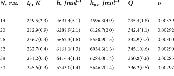
TABLE 1. Results obtained from fitting for experimental data taken from Scholtz et al. (1991). The first column shows chain length (in repeated units), and the next four columns show fitting parameters, described in the text; numbers in brackets show errors in percentages. Nucleation parameter σ is recalculated as 1/Q. For all fits, the coefficient of determination is R² = 0.999. Energies are measured in Joules per mole and temperature in Kelvins.

FIGURE 1

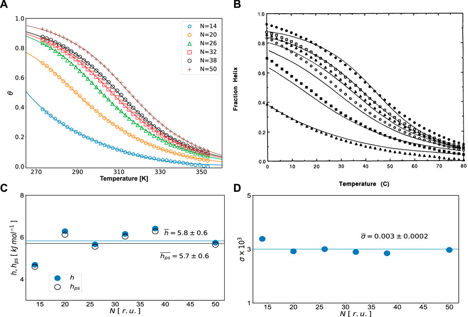
FIGURE 1. (A) Helicity degrees for different chain lengths (N, r.u.). The data points (symbols) are taken from Scholtz et al. (1991). Solid lines are fits of Eq. 18 to experimental data. Fitting values are reported in Table 1: (B) fraction helix (helicity degree) data with original fits reproduced from Figure 3 of Scholtz et al. (1991) (with permission from Biopolymers journal), (C) inter- (h_ps) and intramolecular (h) H-bonding energies, and (D) nucleation parameter σ vs. N. Averages and standard deviations are shown in the graph.

As one can see from Table 1, the overall quality of fit is very good, the value of the coefficient of determination is R² = 0.999, and errors of fitted quantities are small. Not surprisingly, from Figure 1, an excellent fit to experimental data is seen much better than in the original article (Scholtz et al., 1991). All the energies, obtained from the fit, fall within the range of values expected for hydrogen bonding in polypeptides. They cannot be compared to the fit results of Scholtz et al. (1991), since the theory they used did not contain any quantities of solvent and reports only one energy. Instead, our approach, in addition to the intramolecular (inside polypeptide) hydrogen bonding energy h, accounts for the intermolecular (polypeptide-solvent) energy h_ps. Since for all chain lengths considered, h > h_ps, no cold denaturation can take place in the system, although the suggested approach is applicable for the case of cold denaturation as well (Badasyan et al., 2021). The only quantity, which can be directly compared, is the nucleation parameter, for which we got an averaged value of σ = 0.003, practically equal to the value 0.0029 reported in Table 1 of Scholtz et al. (1991).

Another study of helix–coil transitions in Ala-based polypeptides of different lengths was performed by Wang et al. (2004). The mean residue ellipticity [θ]₂₂₂ at 222 nm as a function of temperature can be converted to helicity degree using the following convention (Wang et al., 2004):

$\begin{array}{c}{\theta }_H=-44000\cdot \left(1-x/n\right)+100T\\ {\theta }_C=+640-45\cdot T\\ \theta =\frac{{\left[\theta \right]}_{222}-{\theta }_C}{{\theta }_H-{\theta }_C}.\end{array}(20)$

n is the number of repeat units in the chain; x is a constant equal to 2.5, used for correction of non-hydrogen bonded carbonyls not contributing to θ_H (Wang et al., 2004).

Here again, we fit our Eq. 18 (Wang et al., 2004) to data points. Results of the fit are presented in Table 2 and Figure 2.

TABLE 2

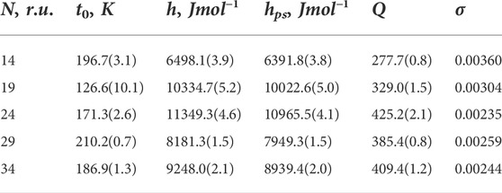
TABLE 2. Results obtained from fitting for experimental data taken from Wang et al. (2004). Quantities and units same as in Table 1. For all fits, the coefficient of determination is R² = 0.999.

FIGURE 2

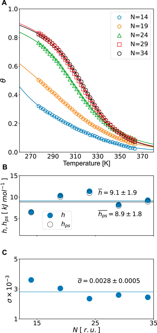
FIGURE 2. (A) Helicity degrees for different chain lengths (N, r.u.). The data points were taken from Ting Wang et al. (2004). Solid lines are fits of experimental data using Eq. 18. Fitted values from Table 2: (B) inter- (h_ps) and intramolecular (h) H-bonding energies and (C) nucleation parameter σ vs. N. Averages and standard deviations are shown in the graph.

We again see a very good overall quality of fit with R² = 0.999 and small errors of fitted quantities. The energies, obtained from the fit, fall within the range of values, expected for hydrogen bonding in polypeptides. However, these energies are certainly higher for polyAla sequences of Ting Wang et al. (2004), as compared to Glu, Lys, and Ala mixtures of Scholtz et al. (1991). In both Figures 1B and 2B, h and h_ps values are close to each other. On the one hand, this is as expected: both are H-bonding energies. On the other hand, it is surprising how close these energies are; a small alteration of the balance can bring global changes. As to the nucleation parameter, it shows a wider span of values around σ = 0.003. Ting Wang et al. (2004) reported the value of σ = 0.002, resulting from fitting the kinetic data. We see it reasonably close to our value, considering that the models used are different.

The same approach, as we have shown in our recent publication (Badasyan et al., 2021), can also fit cold denaturation data, but since h > h_ps for the data considered, cold denaturation is not observed.

Ren et al. (2017) performed helix–coil experiments with synthetic homopolypeptide samples of different lengths. The results were compared with the Schellman and ZB models. For short chains, the ZB model was reported to fit well, while for longer chains, the authors reported that fit was not achieved. When trying to reproduce their results, we noted certain inconsistencies with the experimental data reported in Ren et al. (2017). For instance, it is not clear whether refer to the helicity degrees or fractions of denaturation. When comparing Zimm and Bragg (1959), Scholtz et al. (1991), and Wang et al. (2004), the transition curves have opposite behaviors. Anyway, even corrected, the fit is not converging or is very poor for the Ren et al. (2017) data, with either their formulas or our expression Eq. 18 (Wang et al., 2004). For the abovementioned reasons, we have excluded their data from consideration.

3.2 Transition temperature and interval analysis

The fitted curves of helicity degree we have obtained can be used to calculate transition temperatures and transition intervals from Eq. 6 to Eq. 7 for every chain. This way we can obtain the size scaling of these relevant quantities.

Transition temperature $T_m^N$ for finite chains of length N can be found using the Eq. 6 (Neelamraju et al., 2015) condition. For infinite chains, the transition temperature $T_m^{\infty }$ can be estimated by inserting $\tilde{s}=1-2\sigma$ in Eq. 17 (Ren et al., 2017).

Transition interval ΔT^N for finite chains is found in Eq. 7 (Schreck and Yuan, 2011). Its infinite chain limit expression ΔT^∞ can be estimated analytically as $4\sqrt{\sigma }$.

As shown in Figure 3, fitted experimental curves follow the size-scaling trends in both transition interval and temperature, as reported of Badasyan (2021) recently. Moreover, at all chain lengths considered in Scholtz et al. (1991), systems are beyond the single-sequence approximation but below the limit of long chains for the Zimm–Bragg model.

FIGURE 3

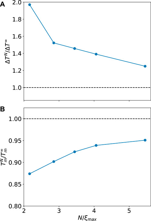
FIGURE 3. Transition interval and temperature in relative units over a range of reduced chain lengths for the transition data obtained from Scholtz et al. (1991). As we see, there are five correlation lengths and the finite size effects are still strong.

4 Conclusion

We have extended the application of the Zimm–Bragg model to the simultaneous account of chain length and solvent effects. Using derived formulas, we successfully analyze the experimental data for the set of two polypeptides and show a better fit as compared to the originally reported one. As a result, it became clear that the poor fit reported in Scholtz et al. (1991) and Wang et al. (2004) can be overcome by a detailed analysis of the size and solvent effects. Last but not least, we confirm once more the statement made in Badasyan (2021) that in many real-world applications and nanobiotechnologies, the characteristic chain lengths fall between those of a single-sequence approximation and a long-chain limit. It means special care should be taken when estimating the stabilities of short polypeptides.

Although we have neglected the effects arising from the difference in amino acid sequences and related charges, our approach represents an improvement over previous approaches and allows us to achieve better fitting of the experimental data, suggesting that our fitting parameters account in an implicit way for the average effect of sequence and charges for small polypeptides (Schiro and Weik, 2019;Mallamace et al., 2016).

Data availability statement

The data analyzed in this study is subject to the following licenses/restrictions: data were digitized from the published manuscripts and properly cited in the body of manuscript. Requests to access these datasets should be directed to abadasyan@gmail.com.

Author contributions

AB and KY designed and developed the overall method and approach. AB and MV supervised the research. KY and AB wrote the code and analyzed the data. KY and AB wrote the article. All authors read and commented on the article.

Acknowledgments

Authors acknowledge financial support from the Slovenian Research Agency through program P2-0412.

Conflict of interest

The authors declare that the research was conducted in the absence of any commercial or financial relationships that could be construed as a potential conflict of interest.

Publisher’s note

All claims expressed in this article are solely those of the authors and do not necessarily represent those of their affiliated organizations, or those of the publisher, the editors, and the reviewers. Any product that may be evaluated in this article, or claim that may be made by its manufacturer, is not guaranteed or endorsed by the publisher.

References

Adam, G., and Gibbs, J. H. (1965). On the temperature dependence of cooperative relaxation properties in glass-forming liquids. J. Chem. Phys. 43, 139–146. doi:10.1063/1.1696442

CrossRef Full Text | Google Scholar

Ananikyan, N. S., Hajryan, S. A., Mamasakhlisov, E. S., and Morozov, V. F. (1990). Helix-coil transition in polypeptides: A microscopical approach. Biopolymers 30, 357–367. doi:10.1002/bip.360300313

CrossRef Full Text | Google Scholar

Badasyan, A. (2021). System size dependence in the zimm–bragg model: Partition function limits, transition temperature and interval. Polymers 13 (12), 1985. doi:10.3390/polym13121985

PubMed Abstract | CrossRef Full Text | Google Scholar

Badasyan, A. V., Giacometti, A., Mamasakhlisov, Y. Sh., Morozov, V. F., and Benight, A. S. (2010). Microscopic formulation of the Zimm-Bragg model for the helix-coil transition. Phys. Rev. E 81, 021921. doi:10.1103/physreve.81.021921

PubMed Abstract | CrossRef Full Text | Google Scholar

Badasyan, A. V., Tonoyan, Sh. A., Mamasakhlisov, Y. Sh., Giacometti, A., Benight, A. S., and Morozov, V. F. (2011). Competition for hydrogen-bond formation in the helix-coil transition and protein folding. Phys. Rev. E 83, 051903. doi:10.1103/physreve.83.051903

PubMed Abstract | CrossRef Full Text | Google Scholar

Badasyan, A. V., Tonoyan, Sh. A., Giacometti, A., Podgornik, R., Parsegian, V. A., Mamasakhlisov, Y. Sh., et al. (2014). Unified description of solvent effects in the helix-coil transition. Phys. Rev. E 89, 022723. doi:10.1103/physreve.89.022723

PubMed Abstract | CrossRef Full Text | Google Scholar

Badasyan, A., Tonoyan, S., Valant, M., and Grdadolnik, J. (2021). Implicit water model within the Zimm-Bragg approach to analyze experimental data for heat and cold denaturation of proteins. Commun. Chem. 4, 57. doi:10.1038/s42004-021-00499-x

CrossRef Full Text | Google Scholar

Goldstein, R. E. (1984). Potts model for solvent effects on polymer conformation. Phys. Lett. A 104, 285–289. doi:10.1016/0375-9601(84)90072-0

CrossRef Full Text | Google Scholar

Hwa Chan, K., Lee, W. H., Zhuo, S., and Ni, M. (2017). Harnessing supramolecular peptide nanotechnology in biomedical applications. Int. J. Nanomedicine 12, 1171–1182. doi:10.2147/ijn.s126154

PubMed Abstract | CrossRef Full Text | Google Scholar

Loo, Y., Zhang, S., and Hauser, C. A. E. (2011). From short peptides to nanofibers to macromolecular assemblies in biomedicine. Biotechnol. Adv. 30 (3), 593–603. doi:10.1016/j.biotechadv.2011.10.004

PubMed Abstract | CrossRef Full Text | Google Scholar

Mallamace, F., Corsaro, C., Mallamace, D., Vasi, S., Vasi, C., Baglioni, P., et al. (2016). Energy landscape in protein folding and unfolding. PNAS 113, 3159–3163. doi:10.1073/pnas.1524864113

PubMed Abstract | CrossRef Full Text | Google Scholar

Neelamraju, S., Oakley, M. T., and Johnston, R. L. (2015). Chiral effects on helicity studied via the energy landscape of short (D, L)-alanine peptides. J. Chem. Phys. 143, 165103. doi:10.1063/1.4933428

PubMed Abstract | CrossRef Full Text | Google Scholar

Ren, Y., Baumgartner, R., Fu, H., Schoot, van der P., Cheng, J., and Lin, Y. (2017). Revisiting the helical cooperativity of synthetic polypeptides in solution. Biomacromolecules 18 (8), 2324–2332. doi:10.1021/acs.biomac.7b00534

PubMed Abstract | CrossRef Full Text | Google Scholar

Schiro, G., and Weik, M. (2019). Role of hydration water in the onset of protein structural dynamics. J. Phys. Cond. Mat. 31, 463002. doi:10.1088/1361-648X/ab388a

PubMed Abstract | CrossRef Full Text | Google Scholar

Scholtz, J. M., Qian, H., York, E. J., Stewart, J. M., and Baldwin, R. L. (1991). Parameters of helix-coil transition theory for alanine-based peptides of varying chain lengths in water. Biopolymers 31 (13), 1463–1470. doi:10.1002/bip.360311304

PubMed Abstract | CrossRef Full Text | Google Scholar

Schreck, J. S., and Yuan, J. M. (2011). A statistical mechanical approach to protein aggregation. J. Chem. Phys. 135, 235102. doi:10.1063/1.3666837

PubMed Abstract | CrossRef Full Text | Google Scholar

Tong, L., Lu, X. M., Zhang, M. R., Hu, K., and Li, Z. (2022). Peptide-based nanomaterials: Self-assembly, properties and applications. Bioact. Mater. 11, 268–282. doi:10.1016/j.bioactmat.2021.09.029

PubMed Abstract | CrossRef Full Text | Google Scholar

Wang, T., Zhu, Y., Getahun, Z., Du, D., Huang, C. Y., DeGrado, W. F., et al. (2004). Length dependent helix–coil transition kinetics of nine alanine-based peptides. J. Phys. Chem. B 108 (39), 15301–15310. doi:10.1021/jp037272j

CrossRef Full Text | Google Scholar

Wood, G. G., Clinkenbeard, D. A., and Jacobs, D. J. (2011). Nonadditivity in the alpha-helix to coil transition. Biopolymers 954, 240–253. doi:10.1002/bip.21572

PubMed Abstract | CrossRef Full Text | Google Scholar

Zimm, B. H., and Bragg, J. K. (1959). Theory of the phase transition between helix and random coil in polypeptide chains. J. Chem. Phys. 31, 526–535. doi:10.1063/1.1730390

CrossRef Full Text | Google Scholar