Combination of Genome-Scale Models and Bioreactor Dynamics to Optimize the Production of Commodity Chemicals

The current production of a number of commodity chemicals relies on the exploitation of fossil fuels and hence has an irreversible impact on the environment. Biotechnological processes offer an attractive alternative by enabling the manufacturing of chemicals by genetically modified microorganisms. However, this alternative approach poses some important technical challenges that must be tackled to make it competitive. On the one hand, the design of biotechnological processes is based on trial-and-error approaches, which are not only costly in terms of time and money, but also result in suboptimal designs. On the other hand, the manufacturing of chemicals by biological processes is almost exclusively carried out by batch or fed-batch cultures. Given that batch cultures are expensive and not easy to scale, technical means must be developed to make continuous cultures feasible and efficient. In order to address these challenges, we have developed a mathematical model able to integrate in a single model both the genome-scale metabolic model for the organism synthesizing the chemical of interest and the dynamics of the bioreactor in which the organism is cultured. Such a model is based on the use of Flexible Nets, a modeling formalism for dynamical systems. The integration of a microscopic (organism) and a macroscopic (bioreactor) model in a single net provides an overall view of the whole system and opens the door to global optimizations. As a case study, the production of citramalate with respect to the substrate consumed by E. coli is modeled, simulated and optimized in order to find the maximum productivity in a steady-state continuous culture. The predicted computational results were consistent with the wet lab experiments.

1 Introduction

Methyl methacrylate (MMA) is a volatile synthetic chemical used mainly in the preparation of acrylic emulsion and extrusion resins. Polymers and co-polymers containing methyl methacrylate are used as solvents, adhesives, sealants, leather and paper coatings, inks, textiles, dental prothesis, etc.

There are 17 different routes widely used in industry that end up synthesizing MMA. The main problem with these routes is that all the precursor molecules (ethylene, propyne, propylene, tert-butyl alcohol, isobutene and isobutane) have their origin in non-renewable sources such as petroleum and natural gas whose extraction is highly damaging for ecosystems (Sugiyama et al., 2009).

An alternative approach consists of considering citramalate, a precursor for the synthesis of MMA, which is produced by Methanocaldococcus jannaschii. The production of citramalate in M. jannaschii is due to the presence of the gene cimA which encodes the enzyme citramalate synthase (EC: 2.3.1.182). This enzyme catalyses the reaction in which one molecule of acetyl-CoA, one molecule of pyruvate and one molecule of water react to produce one molecule of (3 R)-citramalate, one molecule of CoA and liberating a proton (UniProt Consortium, 2019):

$acetyl-CoA+pyruvate+H_{2}O\to \left(3R\right)citramalate+CoA+H^{+}(1)$

One of the most difficult tasks when carrying out the design of a biological experiment is setting the conditions and parameters that have to be tracked during the experiment. Computational models can help overcome these difficulties by providing the researchers with guidance when designing experiments in the wet lab, thus avoiding costly trial-and-error approaches.

In Webb et al. (2018), researchers could reach an efficient bioproduction of citramalic acid by a genetically engineered E. coli strain which included the gene CimA. The fact that the cell culture operated in fed-batch mode suggests that the production could be optimized by changing to continuous culture. In a continuous culture, a steady state is reached when the macroscopic variables of the tank remain constant over time. The complexity of continuous cultures lies in the fact that identical macroscopic conditions may trigger multiple steady states. The potential steady states of an E. coli continuous culture are characterized in Fernandez-de Cossio-Diaz et al. (2017).

Flux Balance Analysis (FBA) Orth et al. (2010) has proven to be an extremely useful approach to analyze steady states of genome-scale constraint-based models. FBA assumes the attainment of a steady state of intracellular metabolite concentrations to compute reactions fluxes by means of a linear programming problem. In addition to analyzing the potential steady states, a challenging problem when modeling and optimizing a continuous culture consists of linking the microscopic variables of the genome-scale model with the macroscopic variables of the bioreactor, e.g., metabolite concentrations out of the cells.

A variation of the FBA approach, called Dynamic Flux Balance Analysis (DFBA) (Mahadevan et al., 2002a), can be used to couple intracellular metabolism with the dynamics of the extracellular metabolite concentrations. DFBA has been applied for the production of several metabolites. In Flassig et al. (2016), the production of β-carotene in green microalgae was optimized for a fed-batch continuous culture. The work in Hanly et al. (2013) validated and optimized a yeast dynamic flux balance model in order to determine the optimum conditions that maximize the production of ethanol in a batch culture of S. cerevisiae. Two approaches to predict batch growth of E. coli based on DFBA are introduced in Mahadevan et al. (2002b). DFBA was applied as well in (Meadows et al. (2010)) with the aim of simulating simultaneous acetate and glucose consumption and evaluate the behaviour of E. coli cells in different types of media. Although DFBA has been applied successfully in many areas, it has some limitations as it assumes quasi-steady-state conditions (Reimers and Reimers,2016) and has been used almost exclusively on batch and fed-batch cultures.

Other methods not based on DFBA, such as k-OptForce, have been used to integrate kinetics in constraint-based models. For instance, the optimization of the production of L-serine in mutant E. coli and triacetic acid lactone in mutant S. cerevisae were performed in Chowdhury et al. (2014). K-OptForce uses kinetic rate expressions to redistribute fluxes in the metabolic network, instead of relying on surrogate fitness functions such as biomass maximization. For additional information on this topic, a review of efforts to integrate kinetic information in constraint-based models can be found in Kim et al. (2018).

In contrast to the previous works, we propose the use of Flexible Nets (FNs) Júlvez et al., 2018), a modeling framework that produces analytical models that can be represented graphically and that are well suited for analysis and optimization, in order to design an overall computational model that combines both the bioreactor dynamics and the metabolic network of the cultured organism. In addition to facilitating the integration of a macroscopic and a microscopic model, FNs can accommodate uncertain parameters and can approximate non-linear dynamics. In particular, constraint-based models Sigmarsdóttir et al. (2020) of metabolic networks can be straightforwardly mimicked and analyzed by FNs. Notice that such models do not account for the concentration of species, and loose flux bounds are usually associated with the reactions. Moreover, FNs can also model the differential equations that determine the dynamics of the bioreactor variables, e.g., cell density, nutrient supply, and metabolite concentration. In this way, FNs can integrate, in a seamless model, both the genome-scale model of the cultured microorganism and the bioreactor dynamics. We show how such an integrated model can be developed and exemplify the process through the modeling and simulation of a system that produces citramalate by a genetically modified E. coli culture. The optimization of the model obtained with respect to citramalate productivity provides the optimal settings, i.e., intracellular fluxes and bioreactor parameters, that maximize the productivity of citramalate in a steady-state continuous culture.

2 Materials and Methods

2.1 Flexible Nets

Flexible Nets (FNs) is a modeling formalism for dynamic systems inspired by Petri Nets, see Murata (1989); Silva, 1993) for a gentle introduction. FNs aim to capture the relationship between the state and the processes of a given dynamic system by means of two interconnected nets: the event net and the intensity net. On the one hand, the event net models how the processes modify the state variables. On the other hand, the intensity net models how the state variables determine the speeds of the processes. In contrast to Petri nets, both the event and the intensity nets are tripartite graphs which have three types of vertices: places, transitions and handlers. The handlers of the event net are called event handlers, and the handlers of the intensity net are called intensity handlers. Places (which are depicted as circles) are associated with metabolites and transitions (which are depicted as rectangles) are associated with reactions. Event handlers (which are depicted as dots) capture the change of concentration of metabolites produced by reactions. Intensity handlers (also depicted as dots) model how the concentrations of metabolites determine the speeds of reactions. Although event and intensity handlers can be distinguished by the net elements to which they are connected, for clarity the arcs and edges of event handlers will be drawn in black and those of intensity handlers in blue.

As an example, the event net in Figure 1A has four places {A, B, C, D}, two reactions {R₁, R₂} and two event handlers {v₁, v₂}. Such a net models the following reactions:

$\begin{array}{ll}\hfill R_1:& A\to 2C\hfill \\ \hfill R_2:& 2A+B\to D\hfill \end{array}$

FIGURE 1

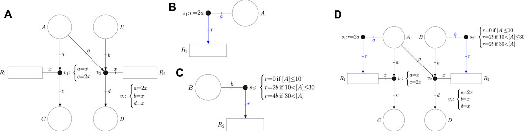
FIGURE 1. (A) Event net modeling the stoichiometry of reactions R₁: A →2 C and R₂2A+ B → D. (B) Intensity net producing a speed in R₁ proportional to the concentration [A]. (C) Guarded intensity net producing a speed in R₂ equal to 0 if [A] is below 10, 2 [B] if [A] is between 10 and 30, and 4 [B] otherwise. (D) Flexible net combining the event net in (A) and the intensity nets in (B) and (C).

The stoichiometry of the reactions is modeled by the equalities associated with the event handlers. In particular, the equalities a = x and c = 2x of v₁ imply that each occurrence of reaction R₁ consumes one unit of metabolite A and produces two units of metabolite C (such units usually refer to concentrations). On the other hand, the equalities a = 2x, b = x, and d = x of v₂ mean that each occurrence of R₂ consumes 2 units of A, 1 unit of B and produces 1 unit of D.

The event net in Figure 1A does not establish any dynamics, it just models the stoichiometry. The dynamics of reactions can be specified by the intensity net. For instance, the intensity net in Figure 1B specifies the speed of reaction R₁ as twice that of the concentration of A, see equation r = 2a associated with the intensity handler s₁. In addition to equalities, intensity handlers can be associated with inequalites to model uncertainty, e.g., if 1.8a ≤ r ≤ 2.2a was associated with s₁ then the speed of R₁ could be any value in the interval [1.8 [A], 2.2 [A]] where [A] is the concentration of A.

Moreover, several sets of equalities and inequalities can be associated with the same intensity handler. If this is the case, the set of inequalities that rules the reaction dynamics is determined by the concentrations of the system. The intensity net in Figure 1C associates three different equalities with the intensity handler s₂ which imply that the speed of R₂ is 0 if [A] is below 10, 2 [B] if [A] is between 10 and 30, and 4 [B] otherwise. Intensity handler s₂ is said to be guarded, it has three guards (or regions) that can determine the speed of R₂. Guarded handlers can be exploited to approximate non-linear kinetics of reactions.

The event net (Figure 1A) can be combined with the intensity nets (Figure 1B and Figure 1C) to produce an FN (Figure 1D) which models both the stoichiometry and dynamics of the system.

2.2 FNs to Model Constraint-Based Models

A constraint-based model (Varma and Palsson, 1994) can be expressed as a tuple $\{\mathcal{R},\mathcal{M},\mathcal{S},L,U\}$ where $\mathcal{R}$ is the set of reactions, $\mathcal{M}$ is the set of metabolites, $\mathcal{S}\in {\mathbb{R}}^{|\mathcal{M}|\times |\mathcal{R}|}$ is the stoichiometric matrix, and $L,U\in {\mathbb{R}}^{|\mathcal{R}|}$ are lower and upper flux bounds of the reactions (notice that very loose flux bounds can be assigned when no kinetic information is available). The concentrations of metabolites are usually disregarded in constraint-based models, being the main focus of most analyses on the fluxes of reactions. This section shows how constraint-based models can be expressed graphically and analyzed numerically in a straightforward way by FNs.

Consider the constraint-based model defined by Table 1. It consists of four reactions together with their corresponding flux bounds. The FN in Figure 2 models such a constraint-based model. The net has one place per metabolite, one transition per reaction, and one event handler per reaction. The equalities associated with the event handlers model the stoichiometry of the reactions. Since constraint-based models do not account for the concentrations of metabolites, the fluxes of reactions cannot depend on concentrations. Hence, the corresponding FN does not have intensity handlers. The range of potential fluxes of reactions is modeled by a parameter λ₀ that is associated with each transition, e.g. λ₀ [R₁] = 5 in R₁ means that the flux of R₁ will always be equal to 5 mmol gDW⁻¹h⁻¹, and 0 ≤ λ₀ [R₂] ≤ 20 in R₂ implies that the flux of R₂ can be any quantity between 0 and 20 mmol gDW⁻¹h⁻¹.

TABLE 1

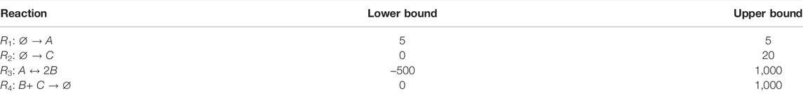
TABLE 1. Simple constraint-based model of four reactions with lower and upper flux bounds (mmol gDW⁻¹h⁻¹). The model is represented graphically by the FN in Figure 2

FIGURE 2

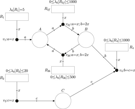
FIGURE 2. FN modeling the constraint based model expressed by the reactions in Table 1. The flux bounds of the reactions are modeled by the default intensities (or speeds) λ₀ of transitions. Reversible reactions like R₃ are unfolded into a forward and a backward reaction with non-negative flux.

The fluxes of transitions must be non-negative in FNs. Thus, the modeling of reversible reactions like R₃ requires its unfolding into two reactions, a forward reaction R_3f and a backward reaction R_3b with appropriate limits for their parameters λ₀ (Júlvez and Oliver, 2020b). If no λ₀ is explicitly associated with a reaction r, then it is assumed that λ₀ [r] = 0. In general, the speed of r is equal to λ₀ [r] plus the intensities provided by the intensity handlers to which it is connected (see Figure 1B).

FNs can be analyzed by building a set of mathematical constraints that the state of the system necessarily satisfies (Júlvez et al., 2018). The association of such constraints with an objective function of interest results in a programming problem whose solution yields a theoretical optimum. For instance, if the objective function for the FN in Figure 2 is the maximization of the flux of R₄ in the steady state, then the solution of the programming problem would be 10 mmol gDW⁻¹h⁻¹ which is the theoretical maximum steady-state flux of R₄. In addition to the flux of R₄, fluxes for the rest of reactions are obtained. In this particular case, this approach is equivalent to performing Flux Balance Analysis (FBA) Orth et al. (2010) on the constraint-based model.

For the production of citramalate, the constraint-based model of the organism Escherichia coli strain K-12 MG1655 (Webb et al. (2018) was considered. The model is named iJO1366 in the BiGG repository database (Orth et al. (2010)) and has 1805 metabolites, 2,583 reactions, and 1,367 genes. The reaction in Eq. 1 was added to this model, simulating a transgenic E. coli strain capable of synthesizing citramalate.

The transformation of the resulting constraint-based model into an FN can be carried out by following the approach to obtain the net in Figure 2. Such an approach is performed automatically by the cobra2fn module of the Python tool fnyzer (Júlvez and Oliver, 2020a).

2.3 FNs to Model Bioreactor Dynamics

The macroscopic model of the bioreactor consists of three parts (see Figure 3) the “Reservoir”, which contains the fresh sterile medium and supplies the cell culture with the essential nutrients for cell survival; the “Tank”, where the cell culture is placed, and the “Effluent” which clears away the accumulated products and some of the cells in the tank.

FIGURE 3

FIGURE 3. Sketch of a bioreactor in continuous culture mode. The nutrient supply and the removal of toxic and cell products are executed at the same time uninterruptedly. The three main compartments are: reservoir, tank and effluent.

The dynamics of the bioreactor variables, which are named macroscopic variables, are determined by differential equations (Fernandez-de Cossio-Diaz et al., 2017). The equation that expresses the evolution of the cell density in the tank is:

$\frac{\mathrm{d}X}{\mathrm{d}t}=\left(\mu -D\right)X(2)$

where X (gDWL⁻¹) is the cell density in the tank, μ is the effective cell growth rate (h⁻¹), and D is the dilution rate (h⁻¹), which is the rate at which culture fluid is replaced divided by the culture volume.

The evolution of the concentration of a given metabolite, i, in the tank is given by:

$\frac{\mathrm{d}{s}_i}{\mathrm{d}t}=\left(c_i-s_i\right)D-u_{i}X(3)$

where c_i is the concentration of the metabolite s in the medium (mM), s_i is the concentration of the metabolite in the tank (mM), D is the dilution rate (h⁻¹), u_i is the specific uptake rate of the metabolite by the cells (mmol gDW⁻¹ h⁻¹), and X is the cell density in the tank (gDW L⁻¹). If u_i > 0 the metabolite is consumed by the cell, otherwise (u_i < 0) the metabolite is secreted from the cell.

For the particular case of a system in which glucose, denoted as metabolite g, is consumed by an E. coli culture, Eq. 3 for the concentration of glucose in the tank becomes:

$\frac{\mathrm{d}{s}_g}{\mathrm{d}t}=\left(c_g-s_g\right)D-u_{g}X(4)$

where c_g is the concentration of glucose in the supply medium, s_g is the concentration of glucose in the tank and, u_g is the glucose uptake flux by the cell (which is a positive value).

The variation of a given product, e.g., citramalate, denoted as c, is derived from Eq. 3 as:

$\frac{\mathrm{d}{s}_c}{\mathrm{d}t}=-s_{c}D-u_{c}X(5)$

where s_c is the citramalate concentration in the tank, and u_c is the citramalate secretion flux. Notice that, since citramalate is secreted from the cell, u_c is negative, and hence, − u_cX is a positive contribution of citramalate to the tank.

The above differential equations can be modeled by FNs.¹ For instance, Eq. 4 can be modeled by the FN in Figure 4 where place G accounts of the concentration of glucose in the tank. As established by Eq. 4, place G has one input flux and two output fluxes. The input flux comes from the reservoir, it is modeled by transition t_gin, and it is equal to D ⋅ c_g. As this is a constant amount, no intensity handlers are needed, and the flux is modeled by the λ₀ associated with t_gin. The output flux modeled by t_gfromtank represents the uptake rate of glucose by the cell culture, and it is equal to u_gX where u_g is the specific uptake rate and X is the cell biomass. This flux is produced by the intensity handler s_ug. Such an intensity handler scales by X the amount of glucose that is consumed by the cells, see equation u_t = uX associated with s_ug. The output flux modeled by t_gout represents the glucose that leaves the tank without being captured by the cells. Such an output flux is equal to the dilution rate times the concentration of glucose in the tank, see equation Ds_g associated with s_gout: r = Ds_g.

FIGURE 4

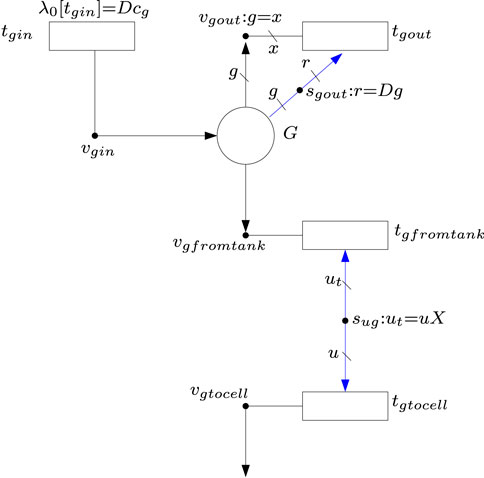
FIGURE 4. FN modeling the differential Eq. 4

Eq. 5 can be modeled similarly by FNs, see place C and the elements connected to it in Figure 5. In this case, there is one input flux and one output flux. The input flux comes from the cell (citramalate is produced by the culture), it is modeled by transition t_ct and it is equal to u_cX, see equation associated with h_c. The output flux corresponds to the amount of citramalate in the tank, once it has been released by the cell, that forms part of the effluent. Such a flux is modeled by t_cout and it is equal to s_cD, see equation associated with s_cout.

FIGURE 5

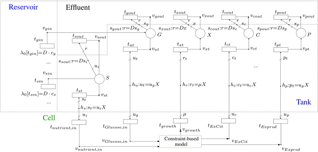
FIGURE 5. FN modeling the overall production system by integrating the macroscopic model of the bioreactor and the microscopic model of the constrained-based model, MODEL1108160000 Orth et al. (2011) of the BioModels database Malik-Sheriff et al. (2020), of the cultured organism.

Finally, Eq. 2 is modeled by the place X and the net elements connected to it. The input flux of X, i.e. the rate at which X increases, is modeled by t_xt and it is equal to the specific growth rate of the culture times the cell density, rX, see equation associated with h_r. The output flux of X, i.e. the rate at which X decreases, corresponds to the cells that are cleared away in the continuous culture, it is modeled by t_xout and is equal to Dx, see equation associated with s_gout.

2.4 Model Integration

The merger of the FNs that model the dynamics of metabolite concentrations in the bioreactor, see Section 2.3, and the FNs that model the constraint-based model of the metabolic network of the cultured organism, see Section 2.2, results in a single FN that models the overall production system, see Figure 5. The nutrients in the medium can be introduced by the transitions located in the reservoir compartment. In this compartment, as many transitions as metabolites in the medium are required. For example, transition t_gin accounts for the presence of glucose in the medium, and transition t_sin represents the presence of a given metabolite s in the medium.

The concentrations of metabolites in the bioreactor are modeled by the places in the tank compartment. In a general system, there will be as many places in the tank compartment as there are metabolites being tracked. In Figure 5, place S represents a generic nutrient, i.e., it is provided by the medium, it is consumed by the culture (see arrow going from S to v_st) and forms part of the effluent. On the other hand, place P represents a generic product, i.e., it is not provided by the medium, it is produced by the culture (see arrow going from S to v_st) and forms part of the effluent. Although the cell density, X, is not a metabolite, its evolution, see Eq. 2, can be modeled exactly as it was a product of the culture, see place X and the net elements connected to it (the increase of X is due to the biomass production which is determined by the growth rate).

For the particular system that produces citramalate by a genetically modified E. coli culture, glucose-limited conditions are assumed. Thus, in addition to the cell density modeled by place X with units gDWL⁻¹, the focus will be on the concentration of one nutrient (glucose which is modeled by place G with units mM), and the concentration of one product (citramalate which is modeled by place C with units mM). Recall that the dynamics of X is ruled by Eq. 2, while G and C are ruled by Eqs 4 and 5, respectively. The microscopic model, i.e., constrained-based model, for the citramalate production system is given by the genome-scale metabolic model of E. coli strain K-12 (iJO1366), MODEL1108160000 Orth et al. (2011) of the BioModels database (Malik-Sheriff et al., 2020). This model was converted to an FN by the fnyzer tool (Júlvez and Oliver, 2020a).

The integration of the macroscopic and the microscopic models was possible thanks to the elements involved in the interface between the tank and the cell compartments. The main elements taking part in this connection are the intensity handlers h_u, h_r and h_c. These intensity handlers relate the macroscopic variables of the bioreactor with the exchange fluxes of the cell in such a way that each macroscopic flux equals X times the exchange flux of the cell, X being the cell density in the tank. The equations which model the interface between the cell and the tank are: u_t = u_gX, r_t = μX, and c_t = u_cX, which are associated with the intensity handlers h_u, h_r and h_c, respectively.

The aforementioned intensity handlers are graphically located at the interface between the cell and tank compartments, and each one acts as a bridge between two transitions: h_u connects t_{Glucose_in} and t_ut, h_r connects t_growth and t_xt, and h_c connects t_ExCit and t_ct. In our model, which contains all the metabolic reactions of E. coli strain K-12 (iJO1366) combined with the reactions that allow citramalate production, t_{Glucose_in} represented the glucose exchange reaction, t_growth is used for the biomass reaction and t_ExCit defined the citramalate exchange reaction.

2.5 Model Optimization

This section discusses the approximations that must be applied to the FN in Figure 5 prior to its optimization (Subsection 2.5.1), as well as the type of objective function that is considered (Subsection 2.5.2).

2.5.1 Tackling Non-linearities

Notice that the equations associated with the intensity handlers at the interface between the macroscopic model of the tank and the microscopic model of the cell are not linear. For instance, the equation associated with h_u is u_t = u_gX where both u_g (the uptake rate of glucose) and X (the cell density) are real variables. The optimization of a non-linear system is, in general, very demanding from a computational point of view. To overcome such a computational burden, non-linear equations can be approximated by piece-wise linear inequalities that are associated with intensity handlers. This approximation results in a guarded FN (see Section 2.1).

A non-linear equation such as u_t = u_gX of h_u can be approximated piece-wise linearly by partitioning the state space of one of the real variables, e.g., X, into a number of regions and associating a linear inequality with each of the regions. Thus, h_u: u_t = u_gX can be approximated by:

$h_u:\left\{\begin{array}{cc}{X}_{min}\cdot u_g\le u_t\le X_1\cdot u_g\hfill & \text{if}{X}_{min}\le X<X_1\hfill \\ X_1\cdot u_g\le u_t\le X_2\cdot u_g\hfill & \text{if}{X}_1\le X<X_2\hfill \\ X_2\cdot u_g\le u_t\le X_3\cdot u_g\hfill & \text{if}{X}_2\le X<X_3\hfill \\ \dots ,\hfill \\ X_{n-1}\cdot u_g\le u_t\le X_{max}\cdot u_g\hfill & \text{if}{X}_{n-1}\le X\le X_{max}\hfill \end{array}\right.(6)$

where X_min and X_max are lower and upper bounds for the cell density, i.e., the cell density is known to be in the interval [X_min, X_max] (notice that these bounds do not need to be tight).

The above approximation considers n regions, the first region is active if the cell density X is in the interval [X_min, X₁] (in general, the ith region is active if the cell density X is in the interval [X_i−1, X_i]). The values X₁, … , X_n−1 do not need to be evenly separated, the only condition they must satisfy is X_min < X₁ < …, < X_n−1 < X_max. This way, one and only one region is active at any particular time. The region that is active determines the linear inequality that is used to produce intensity, i.e., if region i is active then the intensity produced by h_u can be any value in the interval [X_i−1 ⋅ u_g, X_i ⋅ u_g]. Clearly, the higher the number of regions (and hence, the smaller the regions), the better the approximation to the original non-linear equation. Since a higher number of regions involves a longer run time, there is a trade-off between accuracy and computational cost. As discussed below, the number of regions was determined experimentally so that both the computational burden and the obtained precision are acceptable.

Notice that the previously defined regions can also be used to approximate the non-linear equations of the other handlers in the interface between the macroscopic and microscopic models because all include X in their equations. Given that the number of regions has a direct impact on the complexity of the programming problem which needs to be solved (the number of binary variables is linear in the number of regions), partitioning X instead of u_g is advantageous from a computational point of view.

The overall procedure to optimize an FN that integrates a bioreactor and a metabolic network is outlined in Figure 6. After integrating both models in a single FN, a set of mathematical constraints that represent necessary reachability conditions for the state of the system are derived. Such a set of constraints can be derived automatically by the Python tool fnyzer (Júlvez and Oliver, 2020a). The addition of an objective function to the constraints results in a mixed-integer linear programming (MILP) problem whose solution represents the theoretical optimum state that the system can achieve.

FIGURE 6

FIGURE 6. Pipeline showing the steps performed to optimize the integrated model. (1) The metabolic model and the bioreactor dynamics are combined to generate a Flexible Net that integrates the macroscopic (dilution rate, substrate concentration, cell density) and microscopic variables (intracellular metabolite fluxes). (2) A set of mathematical constraints is derived from the net specification and (3) the objective function is selected. The tool fnyzer performs the generation of a mixed-integer linear programming problem according to the set of constraints and the objective function. (4) Finally, the MILP problem is easily solved by using a solver (e.g., CPLEX, Gurobi, GLPK) that computes the mathematical solution.

In order to speed up the model optimization, a non-guarded FN has been defined for each of the above regions, and each of these nets has been solved separately. For instance, region i determines an FN in which the value of X is constrained to the interval [X_i−1, X_i] (this constraint will be part of the programming problem) and the inequalities X₂ ⋅ u_g ≤ u_t ≤ X₃ ⋅ u_g are associated with h_u (similar inequalities are associated with the rest of handler in the interface). The programming problem associated with each of these nets is linear, and hence, can be solved very efficiently. The optimum solution of the original guarded FN can be obtained straightforwardly by taking the maximum of all the computed objective values of the particular non-guarded FNs.

In order to partition the cell concentration X in an appropriate number of regions, the productivity on substrate (PS), see Subsection 2.5.2, was calculated repeatedly for different number of regions, ranging in the interval [10, 200], and fixed values of glucose concentration in the medium, 10 gL⁻¹, and dilution rate, 0.23 h⁻¹. The obtained maximum PS are shown in Figure 7 and the CPU run-times are reported in Supplementary Data S3. Notice that after an initial sharp decrease, the productivity converges to a given value. On the other hand, the run-time of the simulations increases linearly with the number of regions (see reported run-times). Based on these results, it was decided to set the number of regions for the optimizations to 100, as this number provided a good trade-off between accuracy and run-time (the run-time to optimize the FN for a given glucose concentration and a given dilution rate is 564 s (9.4 min), see hardware features in Supplementary Data S3.

FIGURE 7

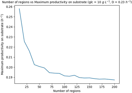
FIGURE 7. Theoretical maximum productivity on substrate PS with respect to the number of regions in which the biomass is partitioned. The glucose concentration is set to 10 g L⁻¹ and the dilution rate to 0.23 h⁻¹.

2.5.2 Optimizing the Productivity

Among the different objective functions that can be considered, we focus on two measures for the productivity of a culture in continuous mode: 1) volumetric productivity, and 2) productivity on substrate.

The volumetric productivity, a. k.a. space-time yield, accounts for the amount of product produced per liter and per hour, it will be denoted VP and is expressed in grams of product per liter per hour, i.e., g ⋅ L⁻¹ ⋅ h⁻¹. In terms of the FN in Figure 5, the volumetric productivity corresponds to the outgoing flux of product flux(P), i.e. intensity of transition t_pout, expressed in g ⋅ L⁻¹ ⋅ h⁻¹. The volumetric productivity would be the primary concern of a chemical engineer designing an industrial process, which needs to be both feasible and economically viable.

The productivity on substrate takes into account both the specific growth rate of the culture, μ (units h⁻¹), and the product yield coefficient, Y_P/S, where Y_P/S denotes the number of grams of product that are produced per Gram of substrate fed into the tank, i.e. $Y_{P/S}=\frac{Product(g)}{Substrate(g)}$, and hence Y_P/S is unitless. In particular, the productivity on substrate, which will be denoted PS, for a given net $\mathcal{N}$ is defined as:

$PS\left(\mathcal{N}\right)=\mu \cdot Y_{P/S}(7)$

given that Y_P/S is unitless, $PS(\mathcal{N})$ is expressed in h⁻¹. Notice that Eq. 7 entails a trade-off between biomass formation and product production. Although the productivity on substrate is usually a secondary concern, it becomes more relevant as the cost of the substrate increases with respect to the selling price of the product. The productivity on substrate is also a useful metric for a synthetic biologist comparing the performance of different genetically engineered microbial strains.

In the following, the mathematical relation between volumetric productivity and productivity on substrate is explored. In a continuous culture, the yield Y_P/S is equal to the grams of product produced per Gram of substrate per time unit, i.e. it can be expressed as $\frac{flux(P)}{flux(S)}$ where flux(P) is the flux of produced product in g ⋅ L⁻¹ ⋅ h⁻¹, and flux(S) is the flux of provided substrate in g ⋅ L⁻¹ ⋅ h⁻¹. Notice that flux(S) is equal to Dc_s where D is the dilution rate in h⁻¹ and c_s is the concentration of the substrate in the fresh medium in g ⋅ L⁻¹. This way, the yield can be expressed as:

$Y_{P/S}=\frac{flux\left(P\right)}{flux\left(S\right)}=\frac{flux\left(P\right)}{D\cdot c_s}(8)$

On the other hand, the cell density is assumed to be constant in a continuous culture, i.e., $\frac{\mathrm{d}X}{\mathrm{d}t}=0$, and hence, Eq. 2 implies that μ = D. Thus, Eq. 7 can be rewritten as:

$PS\left(\mathcal{N}\right)=\mu \cdot Y_{P/S}=D\cdot \frac{flux\left(P\right)}{D\cdot c_s}=\frac{flux\left(P\right)}{c_s}=\frac{VP\left(\mathcal{N}\right)}{c_s}(9)$

Thus, the volumetric productivity is equal to the productivity on substrate times the concentration of substrate in the medium. Therefore, for a given fixed concentration of substrate in the medium, c_s, optimizing the model to maximize productivity on substrate is equivalent to optimizing the model to maximize volumetric productivity. Moreover, for a given c_s, the linear objective function flux(P) can be used to perform such an optimization. For the particular case of citramalate production, flux(P) is given by the value of λ[t_cout] (see Figure 5), and hence, the objective function will be the maximization of λ[t_cout].

2.5.3 Fermentation Experiments

Continuous cultures were grown in a DASbox^® Mini Bioreactor System (Eppendorf, Stevenage, UK). The E. coli strain used for all fermentation experiments was BW25113 ΔldhA pET29a-Cer-BBaJ23119-RFP-cimA3.7. The E. coli ldhA deletion prevents lactate formation, improving flux towards citramalate (Webb et al. (2018)). The plasmid contains both the cimA gene, to enable citramalate production, and the cer gene to reduce loss of the plasmid through mis-segregation (Green et al. (2018)). Glucose-limited chemostat cultures (150 ml working volume) were grown at 37°C, with pH controlled to 7 and dissolved oxygen to $>30\%$, in modified MS (Stephens and Dalton (1987)) medium (2 g L⁻¹ KH2PO4, 2  ml L⁻¹ trace metals solution (Vishniac and Santer (1957), 0.25 ml L⁻¹ antifoam polypropylene glycol, 4 g L⁻¹ NH4Cl, 0.4 g L⁻¹ MgSO4.7H2O). Biomass concentrations were determined by centrifuging measured samples from the fermenter into pre-weighed tubes, washing the pellets, and drying to constant weight at 100°C for 48 h. The supernatants from these samples were used to measure glucose, citramalate, and acetate concentrations. These analyses were performed using an UltiMate 3000 HPLC system (Thermo Fisher Scientific, Loughborough, UK) equipped with an Aminex HPX-87H ion-exclusion column (Bio-Rad, Hertfordshire, UK) and a RefractoMax520 RI detector (Knauer, Berlin, Germany). The mobile phase used was 0.1% (v/v) trifluoroacetic acid (TFA) in Milli-Q water.

3 Results

The validation of the model was carried out by comparing several simulation runs of the designed FN, see Figure 5, to previously obtained experimental results. These experiments were carried out under glucose-limited conditions, using three different concentrations of glucose in the supplied medium (5, 10 and 50 gL⁻¹), and different dilution rates.

Table 2 reports the numerical results obtained both in vivo, and in silico by the FN model. The columns of the table are divided in three parts: the first part sets the experimental parameters, i.e., the glucose concentration in the medium and the dilution rate for the glucose-limited continuous cultures; the second part reports the in vivo experimental results; and the third part reports the in silico results. For each pair of experimental parameters (glucose in medium and dilution rate), the columns corresponding to the “In vivo results” report the cell density (column “Biomass”), the concentration of citramalate (column “Citramalate in tank”), and the concentration of glucose (column “Residual glucose”) measured in the tank. In order to validate the model, the concentrations of citramalate and glucose in the tank are computed for each set of experimental parameters (glucose in medium and dilution rate) and measured biomass. The columns corresponding to the “In silico results” report the computed concentration of citramalate in the tank (column “Citramalate in tank”), the relative error of such predicted concentrations with respect to the measured in vivo concentrations (column “Citramalate relative error”), and the computed concentration of glucose in the tank (column “Residual glucose”).

TABLE 2

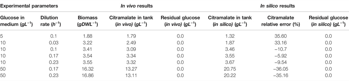
TABLE 2. Data obtained after running the code that simulates the FN model implementing the experimental conditions and previous results.

For a specific concentration of glucose and dilution rate, the biomass and the citramalate concentration reached the values showed in columns “Biomass” and “Citramalate in tank in vivo” of Table 2. From these results, it can be confirmed that the higher the concentration of glucose and dilution rate, the greater the amount of citramalate and biomass that will be produced.

The results obtained for a set of experiments (column “Citramalate in tank in vivo”) are consistent with the results obtained by the simulation of the FN model (column “Citramalate in tank in silico”) for the production of citramalate. The most similar outcome occurs when the glucose concentration was 10 gL⁻¹ as shown in the “Citramalate relative error” column in Table 2.

Notice that, in all cases, the supplied glucose is used up by the culture, i.e. the concentration of residual glucose is 0 gL⁻¹ (column “Residual glucose (in vivo)”). This fact is correctly predicted by the FN model (column “Residual glucose (in silico)”).

Once the model was validated, it was exploited to estimate the theoretical maximum productivity (see Subsection 2.5.2) of citramalate as well as the optimum biomass that produces its associated productivity.

The theoretical maximum volumetric productivity (VP) and productivity on substrate (PS) of citramalate are reported in the heatmaps in Figure 8 and Figure 9, respectively. The cell densities, or biomass concentrations, for which the productivity is optimized are reported in the heatmap in Figure 10. For the explored glucose concentrations and dilution rates, the highest VP was reached when the glucose concentration was 11.0 gL⁻¹ and the dilution rate was 0.51 h⁻¹, such a productivity is obtained with a biomass of 3.14 gDW L⁻¹. With respect to PS, the highest value was obtained for a glucose concentration of 1.0 gL⁻¹ and a dilution rate of 0.51 h⁻¹, such a productivity is obtained with a biomass of 0.275 gDW L⁻¹. It is important to note that the maximum productivities for all concentrations of glucose are obtained when the dilution rate is 0.51 h⁻¹. As expected, the amount of biomass necessary to maximize the productivity increases as the dilution rate and the glucose concentration increase, Figure 10.

FIGURE 8

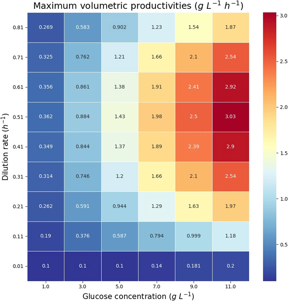
FIGURE 8. Heatmap reporting the maximum volumetric productivities (VPs) for each glucose concentration and dilution rate.

FIGURE 9

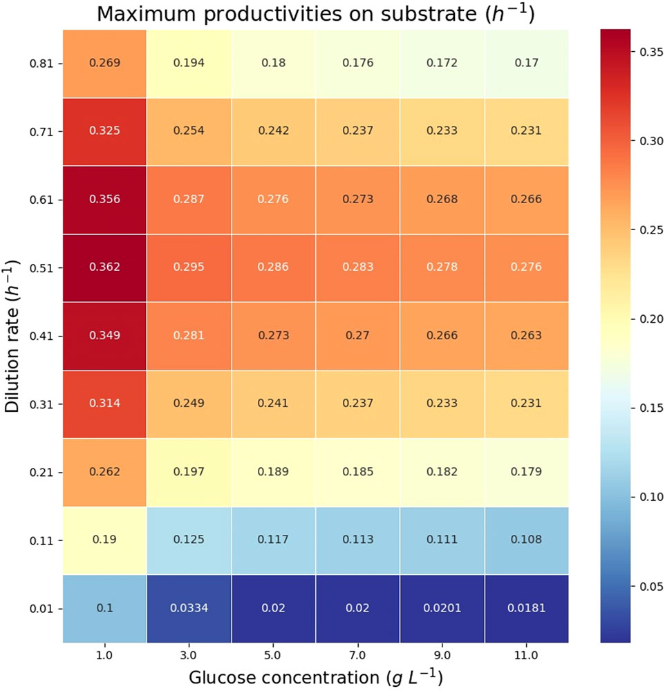
FIGURE 9. Heatmap reporting the maximum productivities on substrate (PS) for each glucose concentration and dilution rate.

FIGURE 10

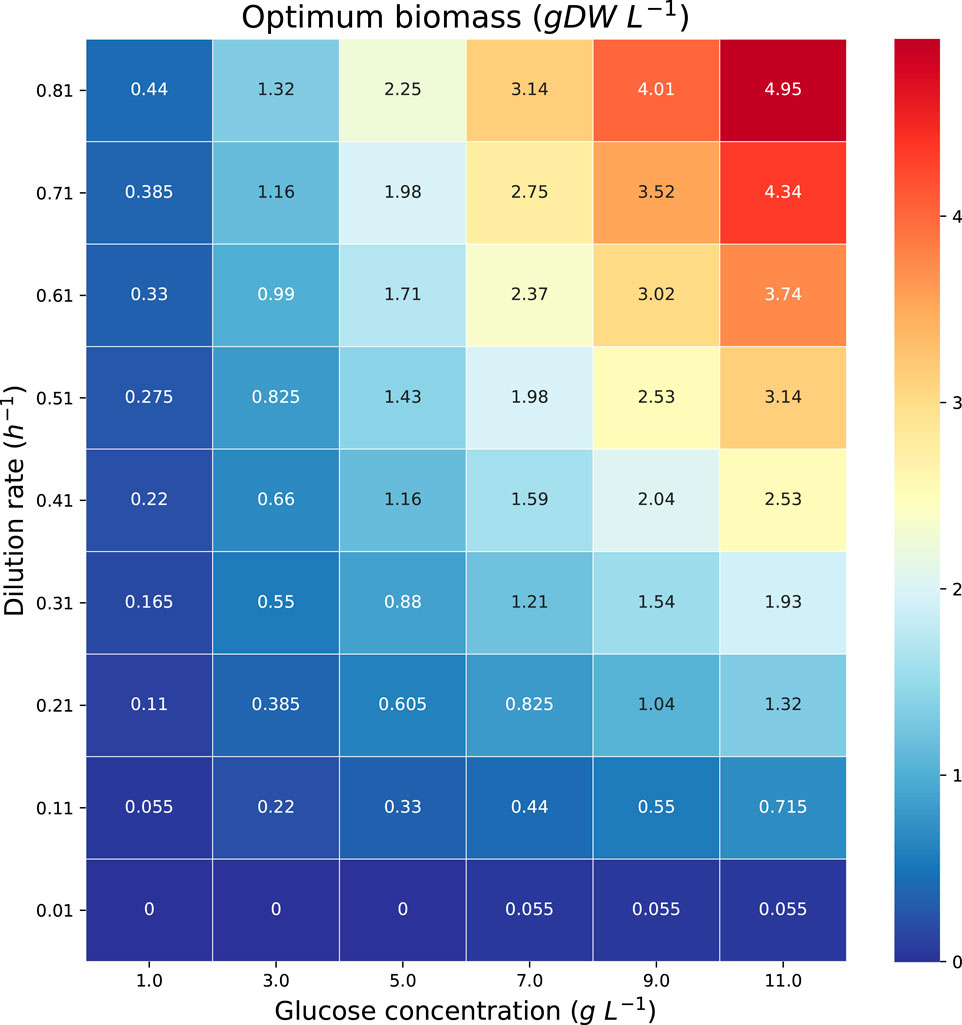
FIGURE 10. Heatmap reporting the optimum biomass concentrations associated with each of the maximum productivities in Figures 8, 9.

The reported in silico results were obtained by fnyzer (Júlvez and Oliver, 2020a) which transforms the FN in Figure 5 into a mixed-integer programming problem, and calls the CPLEX solver (IBM, 2010) to compute the numerical values.

4 Discussion

The mass production of commodity chemicals from fossil fuels can entail a serious negative impact in the environment. As a consequence, alternative approaches are being designed in order to redirect chemical production to more sustainable methods. However, the implementation of these novel approaches at an industrial scale requires optimization before they can replace traditional methods. To achieve this, biotechnology needs to exploit the advantages offered by computational models. Models can provide guidance for the design of experiments, give insights about the underlying mechanisms of the system, perform predictions and rule out infeasible hypotheses. Given the speed at which models can be simulated and optimized, they can save significant amounts of time, effort, and money in the wet lab.

In the last 2 decades, different modeling approaches have been developed, and particular attention has been paid to models of metabolism. In this work, it has been proven that the modeling formalism of FNs can integrate genome-scale constraint-based models, which lack detailed kinetic information, and kinetic models, which account for the concentration of the compounds of the system and are expressed as differential equations. Furthermore, FNs can also accommodate uncertainties inherent to the model, for example, partially unknown parameters.

An FN is represented as the combination of two nets: the event net and the intensity net. The event net models the stoichiometry, whilst the intensity net models the system dynamics. Such a graphical representation produces an overall view of the whole system. The analysis of an FN relies on the solution of a programming problem derived from the FN. If all the reaction rates are linear, i.e., the FN does not have guards, then the resulting programming problem includes only real variables with linear and quadratic constraints that can be solved very efficiently. As a consequence, FNs can handle efficiently genome-scale metabolic networks whose kinetic information is given by flux bounds and linear expressions that define the quantity of metabolites.

In contrast, if the reaction rates are not linear, they need to be approximated by piecewise linear functions, i.e. a guarded FN, which results in programming problems with real and binary variables. The complexity of the algorithms to solve mixed-integer programming problems is exponential in the number of binary variables. In order to obtain a balance between computational burden and accuracy of the model, the number of regions, and hence the number of binary variables, can be modified.

In Section 3, it was shown that FNs are a useful tool to predict the behavior of a complex system, such as a continuous culture in a bioreactor. The predictions of the citramalate production for a specific dilution rate and biomass were reliable in comparison to the experimental results obtained in the in vivo experiments, especially, the ones in which the glucose concentration in the medium was 10 gL⁻¹.

Although the simulations were highly predictive, the model could be improved further by adding some additional information, such as more components in the culture medium, or constraining the uptake of glucose depending on the glucose import rate, and similarly with the citramalate export rate. Both rates depend on protein transporters that can be saturated. Furthermore, the implementation of omics data could improve the model as well (Sánchez et al., 2017).

Not only was this method useful to reproduce the results of the in vivo experiments, but it can also help guide these experiments and optimize the conditions without wasting time and resources. The optimization performed in Section 3 showed that it is of special interest to explore in vivo the conditions that maximized the productivity in the computational simulations.

Data Availability Statement

The Python code generated for this work is available at: https://github.com/jlazaroibanez/opticomch.

Author Contributions

JL, JJ, and SO designed the research; JL, GJ, and JJ developed and implemented the methodology; YY ran the fermentations and generated the experimental data reported; MT-A helped establish initial fermentation conditions; GL oversaw fermentation data collection and analysis; JL, JJ, and SO analyzed and interpreted the results; JL, JJ, and SO wrote the manuscript.

Funding

This work was supported by the Spanish Ministry of Science and Innovation (ref. DAMOCLES-PID2020-113969RB-I00), by a PhD fellowship from Diputación General de Aragón (DGA) (to JL), by the Biotechnology & Biological Sciences Research Council (UK) grant nos. BB/N02348X/1 (to SO) and BB/N023587/1 (to GL), as part of the IBiotech Program, and by the Industrial Biotechnology Catalyst (Innovate UK, BBSRC, EPSRC) to support the translation, development, and commercialisation of innovative Industrial Biotechnology processes.

Conflict of Interest

The authors declare that the research was conducted in the absence of any commercial or financial relationships that could be construed as a potential conflict of interest.

Publisher’s Note

All claims expressed in this article are solely those of the authors and do not necessarily represent those of their affiliated organizations, or those of the publisher, the editors, and the reviewers. Any product that may be evaluated in this article, or claim that may be made by its manufacturer, is not guaranteed or endorsed by the publisher.

Acknowledgments

We are grateful to Giuseppe Nicosia, Cambridge Systems Biology Centre, and to Andrew Yiakoumetti, University of Nottingham, for helpful discussions and comments. The UCL laboratory thanks James Allen for providing the recombinant E. coli strain employed in the fermentation experiments.

Supplementary Material

The Supplementary Material for this article can be found online at: https://www.frontiersin.org/articles/10.3389/fmolb.2022.855735/full#supplementary-material

Supplementary Data | 1. Maximum_Productivities.xlsx: This spreadsheet reports the computed theoretical maximum productivities and their associated cell densities for dilution rates ranging in the interval [0.01, 0.81] h⁻¹ and glucose concentrations in the medium ranging in the interval [1, 11] gL⁻¹.

2. EcolicitFN.xlsx: This spreadsheet reports the fluxes and concentrations for a system with dilution rate D = 0.25 h⁻¹, glucose concentration in the medium glc = 7.0 gL⁻¹ and cell density X = 0.5 gDWL⁻¹. For clarity, only positive fluxes are reported and reactions with null flux are omitted.

3. Regions_and_Runtime.xlsx: This spreadsheet reports the maximum productivity on substrate (PS), optimum biomass, and run-time for a dilution rate of 0.23 h⁻¹, a glucose concentration of 10 gL⁻¹, and a number of regions in the interval [10, 200]. All the simulation results were obtained on a 4 x Intel i5-7200 CPU, 2.50 GHz running Ubuntu 19.10 with 7.7 GB of RAM.

Footnotes

¹For clarity, it is assumed that if the labels and equations of a handler are omitted (see handlers v_gfromtank and v_gtocell in Figure 4), then an equality among all the connected elements holds. For instance if the labels b, c, x and the equation b = c = x are omitted in v₄ in Figure 2, the implicit meaning is that the stoichiometric weights of all metabolites involved in reaction R₄ are 1.

References

Chowdhury, A., Zomorrodi, A. R., and Maranas, C. D. (2014). K-Optforce: Integrating Kinetics with Flux Balance Analysis for Strain Design. Plos Comput. Biol. 10, e1003487. doi:10.1371/journal.pcbi.1003487

PubMed Abstract | CrossRef Full Text | Google Scholar

[Dataset] IBM (2010). IBM ILOG CPLEX Optimizer.

Google Scholar

Fernandez-de-Cossio-Diaz, J., Leon, K., and Mulet, R. (2017). Characterizing Steady States of Genome-Scale Metabolic Networks in Continuous Cell Cultures. Plos Comput. Biol. 13, e1005835. doi:10.1371/journal.pcbi.1005835

PubMed Abstract | CrossRef Full Text | Google Scholar

Flassig, R. J., Fachet, M., Höffner, K., Barton, P. I., and Sundmacher, K. (2016). Dynamic Flux Balance Modeling to Increase the Production of High-Value Compounds in green Microalgae. Biotechnol. Biofuels 9, 165. doi:10.1186/s13068-016-0556-4

PubMed Abstract | CrossRef Full Text | Google Scholar

Green, C. A., Yiakoumetti, A., Allen, J. R., Ward, J. M., and Stephens, G. (2018). Ensuring Sustained Genetic Stability and Productivity during Continuous Culture of E. coli for the Bio-Production of Citramalate. New Biotechnol. 44, 29–30. doi:10.1016/j.nbt.2018.05.128

CrossRef Full Text | Google Scholar

Hanly, T. J., Tiernan, A. R., and Henson, M. A. (2013). Validation and Optimization of a Yeast Dynamic Flux Balance Model Using a Parallel Bioreactor System. IFAC Proc. Volumes 46, 113–118. doi:10.3182/20131216-3-in-2044.00002

CrossRef Full Text | Google Scholar

Júlvez, J., Dikicioglu, D., and Oliver, S. G. (2018). Handling Variability and Incompleteness of Biological Data by Flexible Nets: a Case Study for Wilson Disease. npj Syst. Biol. Appl. 4, 7. doi:10.1038/s41540-017-0044-x

PubMed Abstract | CrossRef Full Text | Google Scholar

Júlvez, J., and Oliver, S. G. (2020b). A Unifying Modelling Formalism for the Integration of Stoichiometric and Kinetic Models. J. R. Soc. Interf. 17, 20200341. doi:10.1098/rsif.2020.0341

CrossRef Full Text | Google Scholar

Júlvez, J., and Oliver, S. G. (2020a). “fnyzer: A Python Package for the Analysis of Flexible Nets,” in 18th International Conference on Computational Methods in Systems Biology (Konstanz, Germany: Springer), 349–355. vol. 12314 of Lecture Notes in Computer Science. doi:10.1007/978-3-030-60327-4_19

CrossRef Full Text | Google Scholar

Kim, O. D., Rocha, M., and Maia, P. (2018). A Review of Dynamic Modeling Approaches and Their Application in Computational Strain Optimization for Metabolic Engineering. Front. Microbiol. 9, 1690. doi:10.3389/fmicb.2018.01690

PubMed Abstract | CrossRef Full Text | Google Scholar

Mahadevan, R., Edwards, J. S., and Doyle, F. J. (2002a). Dynamic Flux Balance Analysis of Diauxic Growth in escherichia Coli. Biophysical J. 83, 1331–1340. doi:10.1016/S0006-3495(02)73903-9

CrossRef Full Text | Google Scholar

Mahadevan, R., Edwards, J. S., and Doyle, F. J. (2002b). Dynamic Flux Balance Analysis of Diauxic Growth in escherichia Coli. Biophysical J. 83, 1331–1340. doi:10.1016/s0006-3495(02)73903-9

CrossRef Full Text | Google Scholar

Malik-Sheriff, R. S., Glont, M., Nguyen, T. V. N., Tiwari, K., Roberts, M. G., Xavier, A., et al. (2020). BioModels-15 Years of Sharing Computational Models in Life Science. Nucleic Acids Res. 48, D407–D415. doi:10.1093/nar/gkz1055

PubMed Abstract | CrossRef Full Text | Google Scholar

Meadows, A. L., Karnik, R., Lam, H., Forestell, S., and Snedecor, B. (2010). Application of Dynamic Flux Balance Analysis to an Industrial escherichia Coli Fermentation. Metab. Eng. 12, 150–160. doi:10.1016/j.ymben.2009.07.006

PubMed Abstract | CrossRef Full Text | Google Scholar

Murata, T. (1989). Petri Nets: Properties, Analysis and Applications. Proc. IEEE 77, 541–580. doi:10.1109/5.24143

CrossRef Full Text | Google Scholar

Orth, J. D., Conrad, T. M., Na, J., Lerman, J. A., Nam, H., Feist, A. M., et al. (2011). A Comprehensive Genome‐scale Reconstruction of Escherichia coli Metabolism-2011. Mol. Syst. Biol. 7, 535. doi:10.1038/msb.2011.65

PubMed Abstract | CrossRef Full Text | Google Scholar

Orth, J. D., Thiele, I., and Palsson, B. Ø. (2010). What Is Flux Balance Analysis? Nat. Biotechnol. 28, 245–248. doi:10.1038/nbt.1614

PubMed Abstract | CrossRef Full Text | Google Scholar

Reimers, A.-M., and Reimers, A. C. (2016). The Steady-State assumption in Oscillating and Growing Systems. J. Theor. Biol. 406, 176–186. doi:10.1016/j.jtbi.2016.06.031

PubMed Abstract | CrossRef Full Text | Google Scholar

Sánchez, B. J., Zhang, C., Nilsson, A., Lahtvee, P. J., Kerkhoven, E. J., and Nielsen, J. (2017). Improving the Phenotype Predictions of a Yeast Genome‐scale Metabolic Model by Incorporating Enzymatic Constraints. Mol. Syst. Biol. 13, 935. doi:10.15252/msb.20167411

PubMed Abstract | CrossRef Full Text | Google Scholar

Sigmarsdóttir, Þ., McGarrity, S., Rolfsson, Ó., Yurkovich, J. T., and Sigurjónsson, Ó. E. (2020). Current Status and Future Prospects of Genome-Scale Metabolic Modeling to Optimize the Use of Mesenchymal Stem Cells in Regenerative Medicine. Front. Bioeng. Biotechnol. 8, 239. doi:10.3389/fbioe.2020.00239

PubMed Abstract | CrossRef Full Text | Google Scholar

Silva, M. (1993). “Introducing Petri Nets,” in Practice of Petri Nets in Manufacturing (Chapman & Hall, London), 1–62. doi:10.1007/978-94-011-6955-4_1

CrossRef Full Text | Google Scholar

Stephens, G. M., and Dalton, H. (1987). The Effect of Lipophilic Weak Acids on the Segregational Stability of Tol Plasmids in pseudomonas Putida. Microbiology 133, 1891–1899. doi:10.1099/00221287-133-7-1891

PubMed Abstract | CrossRef Full Text | Google Scholar

Sugiyama, H., Fischer, U., Antonijuan, E., Hoffmann, V. H., Hirao, M., and Hungerbühler, K. (2009). How Do Different Process Options and Evaluation Settings Affect Economic and Environmental Assessments? a Case Study on Methyl Methacrylate (Mma) Production Processes. Process Saf. Environ. Prot. 87, 361–370. doi:10.1016/j.psep.2009.08.002

CrossRef Full Text | Google Scholar

UniProt Consortium (2019). Uniprot: a Worldwide Hub of Protein Knowledge. Nucleic Acids Res. 47, D506–D515. doi:10.1093/nar/gky1049

PubMed Abstract | CrossRef Full Text | Google Scholar

Varma, A., and Palsson, B. O. (1994). Metabolic Flux Balancing: Basic Concepts, Scientific and Practical Use. Nat. Biotechnol. 12, 994–998. doi:10.1038/nbt1094-994

CrossRef Full Text | Google Scholar

Vishniac, W., and Santer, M. (1957). The Thiobacilli,. Bacteriol. Rev. 21, 195–213. doi:10.1128/br.21.3.195-213.1957

PubMed Abstract | CrossRef Full Text | Google Scholar

Webb, J. P., Arnold, S. A., Baxter, S., Hall, S. J., Eastham, G., and Stephens, G. (2018). Efficient Bio-Production of Citramalate Using an Engineered Escherichia coli Strain. Microbiology 164, 133–141. doi:10.1099/mic.0.000581

PubMed Abstract | CrossRef Full Text | Google Scholar