A lag bloom pattern of phytoplankton after freshwater input events revealed by daily samples during summer in Qinhuangdao coastal water, China

Phytoplankton blooms have become a global concern due to their negative impacts on public health, aquaculture, tourism, and the economic stability of coastal regions. Therefore, elucidating the shifts in phytoplankton community structure and abundance, as well as their environmental drivers, is crucial. However, existing studies often fail to capture the detailed dynamics of phytoplankton blooms and their environmental triggers due to low temporal observation resolution. In this study, high temporal resolution (daily) samples were collected over 43 days to investigate the influence of environmental factors on phytoplankton in Qinhuangdao in the summer. During the observation period, a total of 45 phytoplankton species were identified, comprising 26 Bacillariophyta species, 16 Dinophyta species, 2 Euglenophyta species, and 1 Chromophyta species. Interestingly, a lag bloom pattern of phytoplankton behind freshwater input was observed across day-to-day samples. Phytoplankton blooms typically lagged 1–3 days behind periods of decreased salinity and nutrient input, suggesting that freshwater influx provides the foundational materials and benefits for these blooms. Moreover, the phytoplankton blooms were triggered by six dominant species, i.e., Chaetoceros spp., Pseudo-nitzschia delicatissima, Skeletonema costatum, Protoperdinium spp., Leptocylindrus minimus, Pseudo-nitzschia pungens, and Thalassiosira spp. Consequently, the succession of phytoplankton showed a predominant genera shift in the following sequence: Nitzschia, Protoperdinium, and Prorocentrum – Skeletonema – Pseudo-nitzschia – Gymnodinium – Leptocylindrus. Besides that, a deterministic process dominated phytoplankton community assembly across time series, and DIP is a key factor in shifting the phytoplankton community structures in this area. In summary, our study offers high-resolution observations on the succession of phytoplankton communities and sheds light on the complex and differentiated responses of phytoplankton to environmental factors. These findings enhance our understanding of the dynamics of phytoplankton blooms and their environmental drivers, which is essential for the effective management and mitigation of their adverse impacts.

1 Introduction

Phytoplanktons are fundamental to ecosystem productivity and the structuring of food webs, and they play a pivotal role in the biogeochemical cycling of key elements such as nitrogen, phosphorus, silicon, and carbon on a global scale (Falkowski et al., 1998; Arrigo, 2005; Hilligsøe et al., 2011). However, the rapid urbanization and economic expansion in coastal regions have markedly transformed phytoplankton communities, promoting the proliferation of specific species that can form extensive blooms (Kroeze et al., 2013). These phytoplankton blooms have significant negative impacts on public health, aquaculture operations, tourism, and the economic stability of coastal areas (Genitsaris et al., 2019). It is reported that phytoplankton blooms are estimated to contribute to an annual global medical cost of $30.3 million (Kouakou and Poder, 2019). Therefore, it is crucial to thoroughly understand phytoplankton ecology in coastal waters to enhance the management and conservation of these environments.

Freshwater inputs have been identified as a pivotal factor in the initiation of phytoplankton blooms (Dai et al., 2023; Zeng et al., 2024). Recent investigations using remote sensing technology have documented a global escalation in the frequency of these blooms (Dai et al., 2023). Analogous patterns have been observed in the coastal regions of China, where both large-scale studies highlighted freshwater influxes, predominantly from rainfall, as the most likely catalyst for phytoplankton proliferation (Zeng et al., 2024). Microcosm experiments further corroborate these findings by demonstrating that freshwater inputs can significantly enhance the growth rate, shift the community composition, and change the size structure of phytoplankton populations (Paczkowska et al., 2020). Despite the compelling evidence highlighting the crucial role of freshwater inputs in inducing phytoplankton blooms, the intricate ecological mechanisms underlying these events remain incompletely understood.

Temporal observations are a powerful tool to identify the environmental drivers behind shifts in phytoplankton abundance and communities (Cui et al., 2018; Nunes et al., 2018; Sin and Yu, 2018; Genitsaris et al., 2019). For example, monthly samples collected in Qinhuangdao have shown that salinity, an indicator of freshwater inputs, plays a particularly significant role in regulating the phytoplankton community (Cui et al., 2018). Additionally, weekly samples from estuaries demonstrate that freshwater inputs can impact phytoplankton abundance and community structure by altering physical factors such as hydrodynamic force, turbidity, and salinity, as well as modifying nutrient supply (Sin and Yu, 2018). In the St. Lucia Estuary, changes in salinity and the availability of nitrogen and phosphorus have been identified as key drivers of shifts in the dominant phytoplankton groups (Nunes et al., 2018). Similarly, in urban Thessaloniki Bay, DIP and NH₄⁺ levels are positively correlated with phytoplankton blooms (Genitsaris et al., 2019). Our previous daily sampling efforts also indicated that freshwater inputs significantly influence phytoplankton abundance and community composition, with DIP notably affecting the succession of phytoplankton communities and the blooming of dominant species (He et al., 2022). However, the dynamics of phytoplankton communities and abundance are influenced by a complex interplay of factors. Even within the same area, bloom patterns, community structures, and key environmental drivers can vary from year to year. Therefore, sustained daily sampling is essential to capture the detailed dynamics of phytoplankton community shifts and abundance and to accurately identify their ecological drivers.

Qinhuangdao, located along the Bohai Sea and renowned as a seaside tourist destination in northern China, experiences relatively weak water exchange (Tao, 2006). The region’s coastline is fed by over 17 rivers, which contribute substantial nutrient loads to the coastal waters. Over the past decade, the area has frequently experienced algal blooms, significantly affecting local economic development. These blooms typically begin in April and peak in July (Cui et al., 2018). A particularly notable event was the large-scale brown tide from June to August 2012, which affected 3,400 km² and lasted for 73 days (Zhang et al., 2013). In recent years, smaller algal blooms have also been observed more frequently along the Qinhuangdao coast (Department of Natural Resources of Heibei Province (Ocean Administration), 2023). Thus, Qinhuangdao serves as an excellent region for investigating the ecology of phytoplankton and the dynamics of algal blooms.

In this study, high-resolution time series samples (collected daily) were obtained during the summer, the season with the highest incidence of algal blooms, from a coastal area in Qinhuangdao, China, influenced by a small river. Phytoplankton were identified and counted at the species level using morphological examinations and microscopy. Simultaneously, various environmental factors, including pH, temperature, salinity, and nutrient concentrations, were monitored. The objectives of this study were as follows: (1) to capture the bloom pattern of phytoplankton in the Qinhuangdao coastal area, (2) to reveal the major factors that triggered the blooms and community successions of the phytoplankton, and (3) to provide important insights for developing management strategies to control phytoplankton blooms in coastal waters.

2 Materials and methods

2.1 Study area and water sampling

The sampling site was located in Jinmeng Bay, Qinhuangdao, Hebei Province, and was influenced by the Qiandao River. The island located in the Tang River estuary is an artificial island (Figure 1). Water samples were systematically collected daily from a fixed location between 10 July 2021 and 23 August 2021. Approximately 2.5 L of near-surface seawater (at a depth of 1 m) were gathered each day at 3:00 p.m. All collected samples were immediately placed in a cooler with ice packs, maintaining a temperature of approximately 4°C, and were transported to the laboratory within 2 h for subsequent analysis.

Figure 1

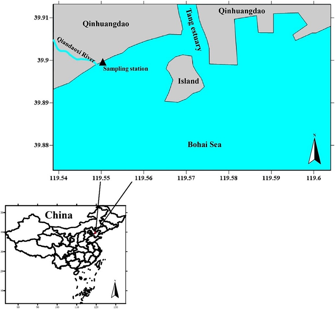
Figure 1. Map of the sampling station (He et al., 2022).

2.2 Environmental parameters

Salinity, water temperature, and pH were measured on-site using a portable multi-parameter water quality monitoring instrument (YSI Pro Series, USA). For nutrient analysis, approximately 500 mL of seawater was filtered through 0.45 μm pore-size membranes. The concentrations of silicate (Si), nitrite (NO₂⁻), nitrate (NO₃⁻), and ammonium (NH₄⁺) were quantified using a QuAAtro nutrient autoanalyzer (Seal Analytical Ltd., Germany), following the methods outlined by He et al. (2019). The combined concentrations of NO₂⁻, NO₃⁻, and NH₄⁺ were utilized to compute the dissolved inorganic nitrogen (DIN) levels. Dissolved inorganic phosphorus (DIP) was monitored in accordance with the “Specification for Oceanographic Survey” (GB/T 12763.4–2007). Rainfall data were sourced from the Chinese Weather Bureau.¹

2.3 Phytoplankton identification

Phytoplankton species were taxonomically identified based on morphological examinations, adhering to the guidelines stipulated in the “Technical Specification for Red Tide Monitoring in China.” Following collection, phytoplankton samples were preserved in 1.5% Lugol’s solution for a minimum of 24 h to facilitate sedimentation of phytoplankton cells. Subsequently, approximately 10 mL of concentrated phytoplankton samples were withdrawn from the bottom layer. Taxonomic determinations and enumeration (cells·L⁻¹) were conducted using a microscope (OLYMPUS CX31, Japan), following the established methodology outlined by Utermöhl (Utermöhl, 1958). Species identification was pursued to the extent possible, with all specimens identified to at least the genus level.

2.4 Data analysis

The phytoplankton species diversity indices of Shannon–Wiener and richness were calculated by vegan package using RStudio (R Development Core Team, 2011). The dominance index (Y) was calculated according to Eq. (1). Non-metric multidimensional scaling (NMDS) was performed by a vegan package using RStudio (R Development Core Team, 2011) to visualize the phytoplankton communities in different groups. Adonis analyses and permutation MANOVAs were applied to test the distinction of phytoplankton in different groups. A mental test was used to analyze the correlation between phytoplankton community structure and environmental factors. Cross-correlation analysis was used to reveal the lag bloom pattern of phytoplankton after freshwater input events using RStudio (R Development Core Team, 2011). The Spearman test was used to analyze the correlation between different environmental factors and dominant species. The taxonomic normalized stochasticity ratio (tNST) was calculated based on the Bray–Curtis distance using the NST package (Ning et al., 2019) in R. The tNST value was used to estimate the ecological stochasticity, with 50% as the cutoff between more deterministic (<50%) and more stochastic (>50%) assemblies.

$\begin{array}{ll}Y=\frac{n_i}{N}\times f_i& (1)\end{array}$

where N represents the number of total species detected during our observation time, n_i represents the abundance of species i, and f_i represents the detectable rate of species i.

3 Results

3.1 Environmental factors

The variations in environmental factors over the day-to-day time series were first analyzed (Figure 2A). The concentrations of DIN, DIP, and Si ranged from 8.50 to 249.79 μmol/L, 0.03 to 2.35 μmol/L, and 26.39 to 435.71 μmol/L, respectively. For physical parameters, salinity, temperature, and pH ranged from 1.87 to 26.82‰, 23.70 to 29.20°C, and 6.48 to 8.42, respectively (Figure 2A). Additionally, there were 17 days of rainfall, with daily precipitation ranging from 0.1 to 160.6 mm.

Figure 2

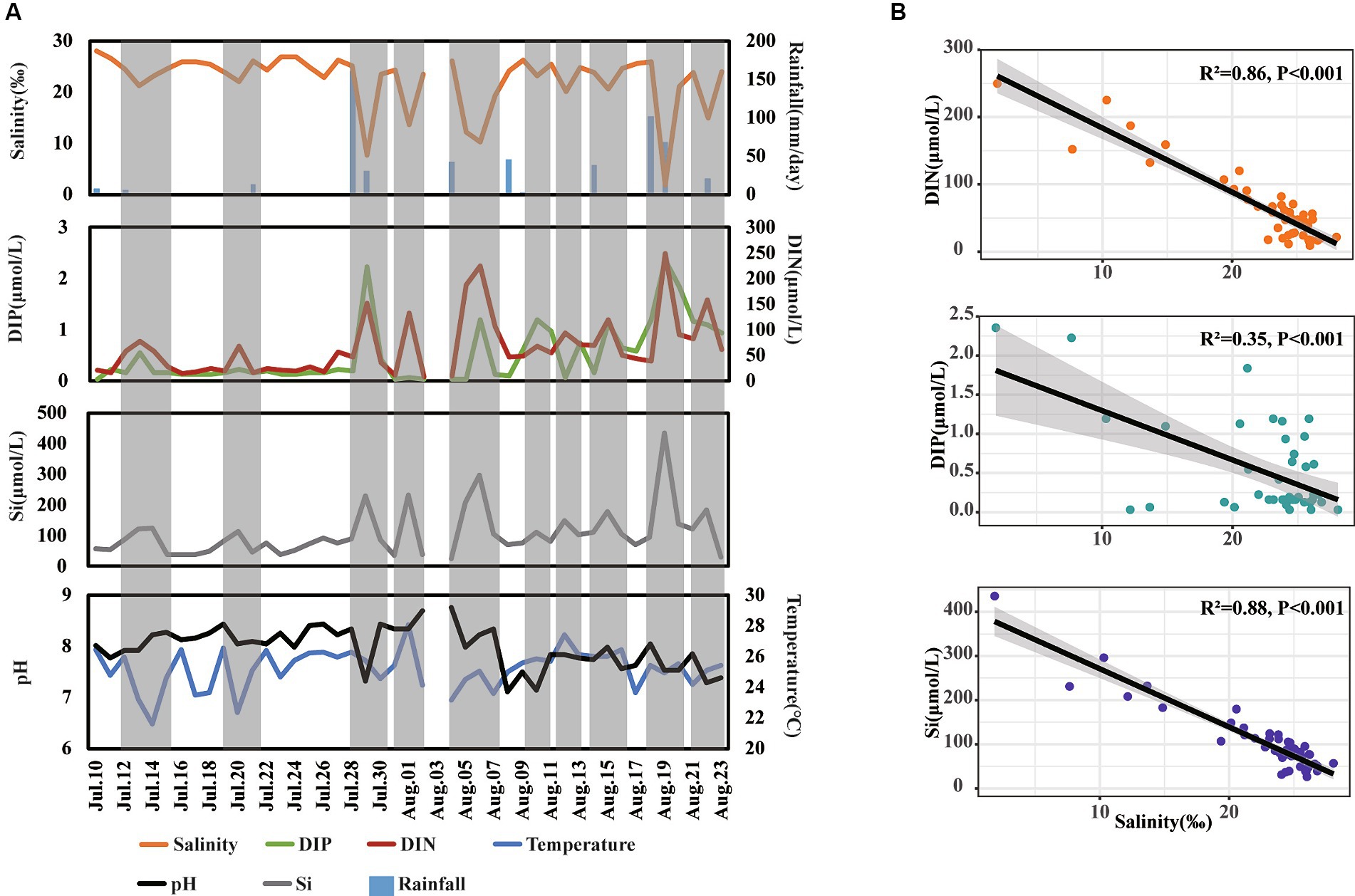
Figure 2. Shift (A) and relationship (B) of different environmental factors across day-to-day time. The gray shadow in panel (A) represents special periods when salinity decreased.

During our observation period, we recorded 10 instances of decreased salinity, indicating freshwater inputs in this area. Notably, during these periods of decreased salinity, the concentrations of DIP, DIN, and Si increased several folds compared to normal days. Furthermore, the concentrations of DIN and Si showed a strong negative correlation with salinity levels (R² > 0.85, p < 0.001), while the concentrations of DIP showed a relatively weaker negative correlation with salinity levels (R² = 0.35, p < 0.001) (Figure 2B) These findings suggest that freshwater inputs significantly enhance nutrient levels, with a more pronounced influence on the concentrations of DIN and Si than on DIP in coastal waters.

3.2 Abundance of phytoplankton

The total abundance of phytoplankton ranged from 2.0 × 10⁴ to 1.49 × 10⁷ cells/L (Figure 3A), which was comparable to our previous study in this field (He et al., 2022). Notably, there were nine phytoplankton bloom events that happened on the 19th, 24th, and 31st of July and the 5th, 7th, 11th, 14th, 21st, and 23rd of August, respectively. Notably, the bloom event was not triggered by the same species. According to the analysis of dominant species (Y > 0.02) abundance (Figure 3A), nine bloom events were triggered by seven dominant species, including Chaetoceros spp., Pseudo-nitzschia delicatissima, Skeletonema costatum, Protoperdinium spp., Leptocylindrus minimus, Pseudo-nitzschia pungens, and Thalassiosira spp. For example, Protoperdinium spp. dominated the bloom events on 19 July and 24 July. Skeletonema costatum and Thalassiosira spp. co-dominated bloom event on 31 July. Furthermore, network analysis (Figure 3C) of those seven species showed that Pseudo-nitzschia delicatissima, leading to a big bloom event on 7 August, significantly positively correlated with other dominant species except Leptocylindrus minimus.

Figure 3

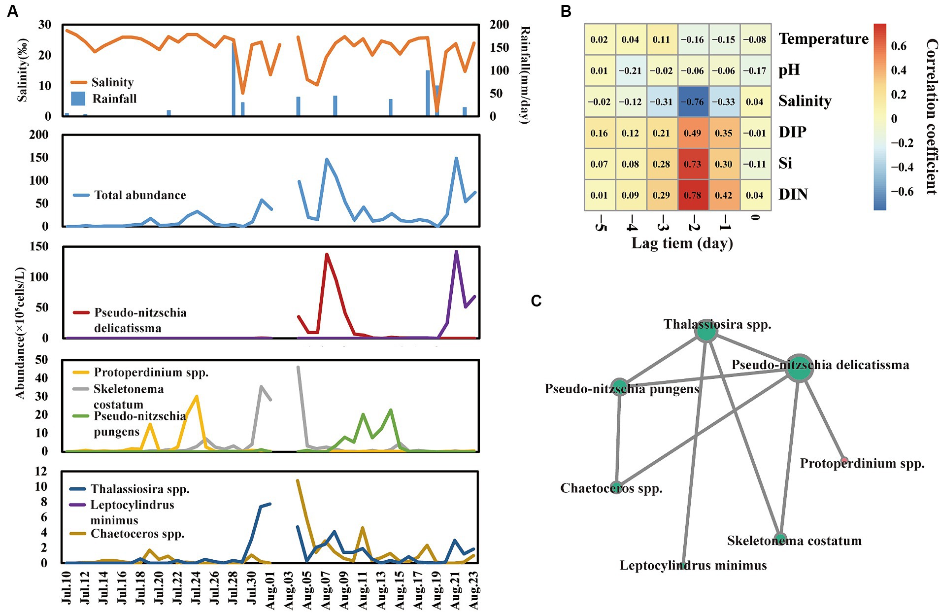
Figure 3. Shift of total phytoplankton and dominant species abundance across time series (A). Cross-correlation analysis (CCA) reveals the lag bloom pattern of total phytoplankton abundance (B). Network reveals the co-relationship among dominant species (C).

Interestingly, a lag bloom pattern of phytoplankton behind freshwater input was observed across day-to-day time samples. Phytoplankton blooms usually lag behind the time of salinity decrease and nutrient inputs. For example, the salinity value dramatically decreased to 1.87 on 19 August, and the abundance of phytoplankton bloomed to 1.49 × 10⁷ cells/L after 2 days. Furthermore, cross-correlation analysis, which could analyze the correlation between a time series and a lagged version of another time series, was used to analyze the lag bloom pattern (Figure 3B). The level of salinity, DIN, Si, and DIP showed a high correlation coefficient with phytoplankton abundance in lag 2 days, suggesting that there is a high likelihood of phytoplankton blooms occurring approximately 3 days after freshwater inputs.

Notably, we also found four potential toxic species (Supplementary Figure S1), including Prorocentrum minimum, Gymnodinium catenatum, Chattonella marina, and Akashiwo sanguinea. Of those four species, Gymnodinium catenatum, Chattonella marina, and Akashiwo sanguinea were occasionally detected and showed a relatively low abundance (<1.00 × 10⁴ cells/L). Nevertheless, Prorocentrum minimum was detected in 16 samples, and the peak abundance was 8.64 × 10⁵ cells/L, which was near to the threshold value (1.00 × 10⁶ cells/L) of red tide according to “Technical specification for red tide monitoring in China.”

3.3 Diversity of phytoplankton

A total of 45 species were detected in Jinmeng Bay during our observation period and 26, 16, 2, and 1 species were divided into Bacillariophyta, Dinophyta, Chromophyta, and Euglenophyta, respectively (Figure 4A). Moreover, Bacillariophyta was detected in all samples, and the number of species belonging to Bacillariophyta ranged from 1 to 10 across time series. Dinophyta was detected in most samples and the number of species belonging to it ranged from 0 to 7 across time series. There is one species belonging to Euglenophyta that was detected in more than half samples. Nevertheless, two Chromophyta species were only detected in three samples.

Figure 4

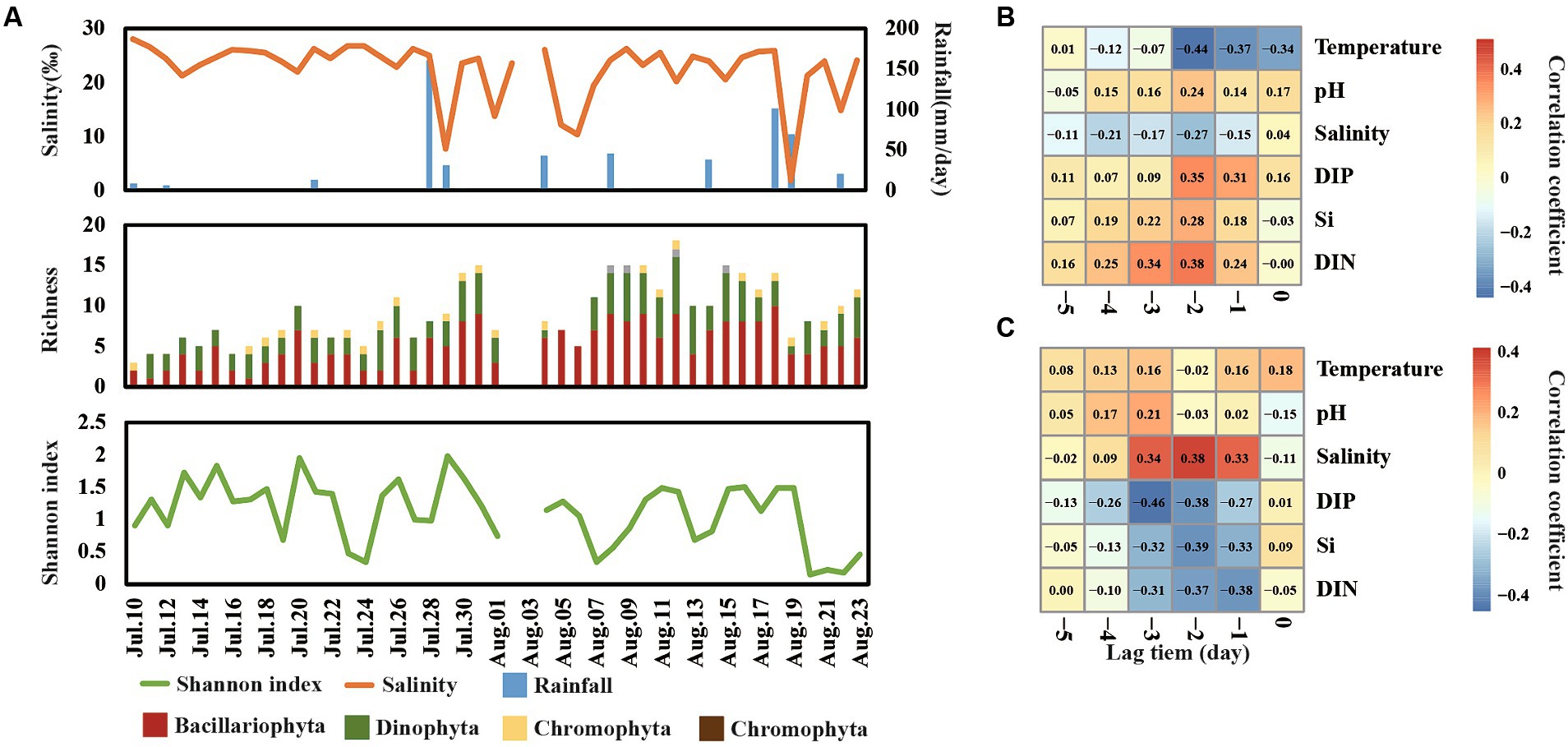
Figure 4. Shift of richness and Shannon index of phytoplankton communities across day-to-day time (A). Cross-correlation analysis (CCA) reveals the lag change pattern of phytoplankton richness (B) and Shannon index (C).

The Shannon index varied from 0.15 to 2.00 in our observation period (Figure 4A). It was notable that the Shannon index showed a significantly negative relationship with the total abundance of phytoplankton. For example, the total abundance of phytoplankton reached a peak on 7 August, while the Shannon index was at a low value on this day. This finding is consistent with our previous studies in this area (He et al., 2022), suggesting that minority species bloom occupied the niche of other phytoplankton and decreased the diversity. Moreover, the level of salinity, DIN, Si, and DIP showed the strongest correlation with richness and Shannon diversity in lag 2–3 days (Figures 4BC), suggesting that most change of diversity would happen in 2 days after the change of salinity, DIN, Si, and DIP.

3.4 Phytoplankton community

Bacillariophyta and Dinophyta were the dominant phyla in our observation period (Figure 5A). Bacillariophyta was the most persistent phylum and was detected in all samples, accounting for more than 85% of the total abundance. As well, Bacillariophyta contributed more than 50% phytoplankton abundance in approximately 70% of samples. Notably, Dinophyta were also detected in most samples and bloomed on some days. For details, Dinophyta was detected in more than 90% of samples and bloomed on 11–25 July and 15–19 August, respectively. Moreover, 12 samples showed more than 50% relative abundance.

Figure 5

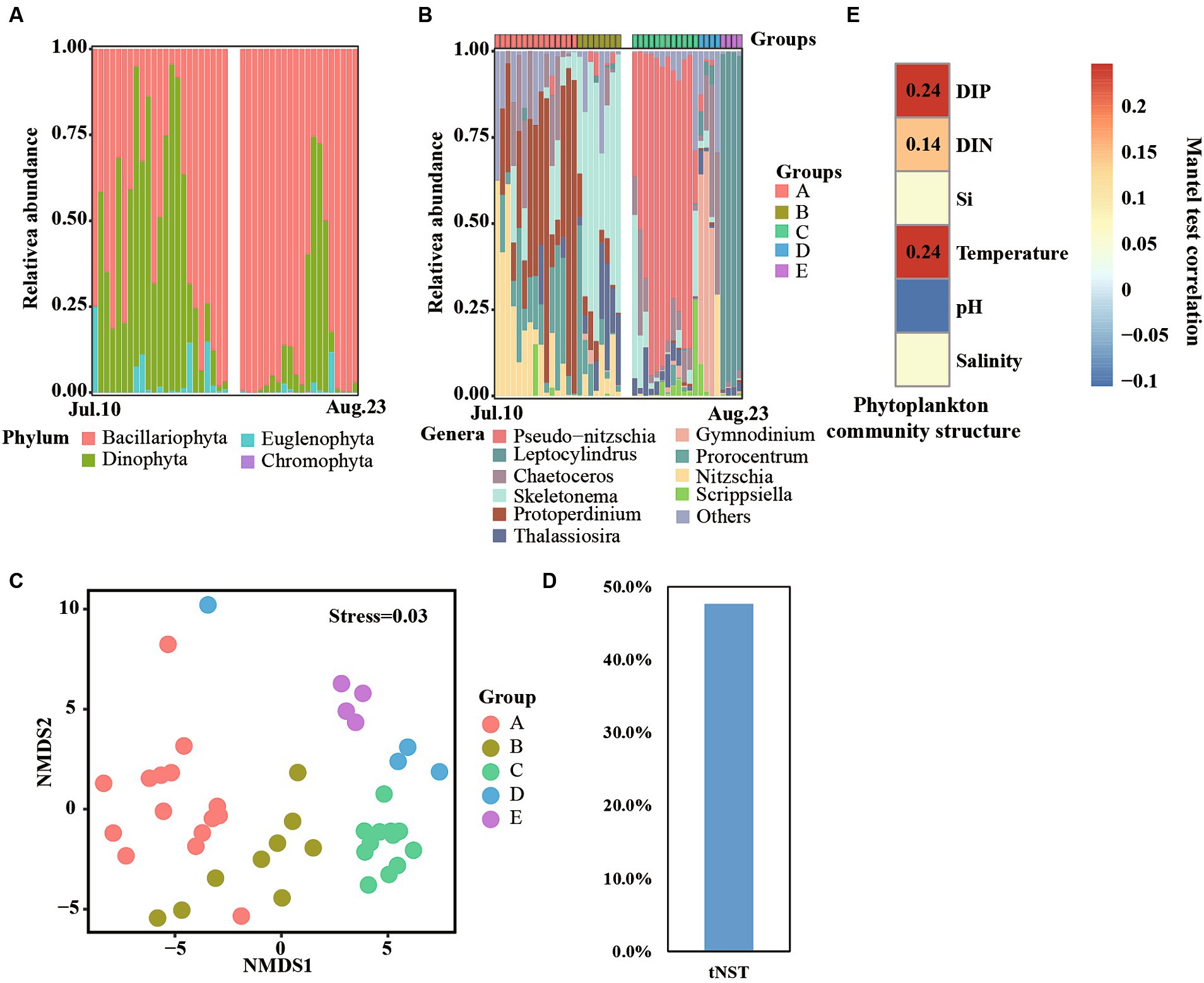
Figure 5. Phytoplankton communities at phylum (A) and genera (B) levels across time series. Non-metric multidimensional scaling (NMDS) reveals different phytoplankton communities (C). Null model analyses reveal the taxonomic normalized stochasticity ratio (tNST) of phytoplankton community assemblages, i.e., the relative importance of stochastic processes in the community assembly across day-to-day samples (D). Mantel test reveals the correlation between phytoplankton community structure and environmental factors (E).

At the genera level, a clear succession progress of the phytoplankton community was observed and the communities were divided into A, B, C, D, and E groups according to the succession of the dominant genera across time series (Figure 5B). For details, samples collected from 10 to 24 July were divided into group A, and Nitzschia, Protoperdinium, and Prorocentrum were the dominant genera of this group. Group B contained samples collected from 25 July—1 August, and Skeletonema was identified as the most abundant genera. Moreover, Protoperdinium, Prorocentrum, and Thalassiosira were also detected in some samples. Samples collected on 4 to 15 August comprised group C, which was dominated by Pseudo-nitzschia. Samples collected on 16–19 August and 20–23 August belonged to groups D and E, respectively. Meanwhile, Gymnodinium and Leptocylindrus dominated the phytoplankton community structure in those two groups, respectively. NMDS analyses also found that all samples were clustered into five groups (Figure 5C), and significant (p < 0.01) differences were observed between them (Supplementary Table S2), which consisted of the results of phytoplankton community structure at the genera level.

The value of tNST, representing the relative importance of stochastic processes in governing taxonomic community structure, was 47% (Figure 5D), lower than 50%, suggesting deterministic selection in governing the taxonomic community structure. Furthermore, significant correlations (p < 0.01, Mantal test) were observed among phytoplankton community structures and DIN, DIP, and temperature (Figure 5E), indicating that these environmental factors influenced the succession of phytoplankton community structures.

4 Discussion

4.1 Lag bloom pattern of phytoplankton behind freshwater input

Phytoplankton blooms have been considered one of the most prevalent ecological problems in coastal regions. In recent years, research has observed an increased trend of phytoplankton bloom frequency on a global scale (Kahru and Mitchell, 2008; Dai et al., 2023). However, the mechanism of this phenomenon still cannot be fully understood. A possible reason is that it is hard to capture environmental factors before phytoplankton bloom, which was considered to play a key role in explaining the phytoplankton blooms. In this study, high-resolution time series samples presented complete data about the progress of phytoplankton blooms, which helps people better understand the mechanism of phytoplankton blooms in coastal regions.

Several studies have demonstrated that phytoplankton blooms are correlated with freshwater inputs and nutrients taken by them. For example, recent research based on remote sensing demonstrated that phytoplankton bloom on a global scale is significantly associated with rainfall events, which led to the high input of freshwater providing abundant nutrients in coastal waters (Dai et al., 2023). However, research has not yet confirmed how long phytoplankton will bloom after freshwater inputs. In this study, we repeatedly observed the association between freshwater inputs and phytoplankton blooms. Furthermore, phytoplankton bloom usually happens in 1–3 days after freshwater inputs in coastal water. The explanation for this phenomenon can be attributed to three reasons. First, freshwater inputs can dilute the phytoplankton, which has been identified as one important factor in regulating phytoplankton abundance in the estuary region. Moreover, this study also found that low levels of phytoplankton abundance and salinity usually cooccurred (Figure 3A). Second, phytoplankton bloom fellows Limiting Factor Principle. Its bloom is a comprehensive progress, which depended on a number of factors, including nutrients (Carstensen et al., 2015), sunlight (Fang et al., 2008), salinity (Gasiūnaitė et al., 2005), water temperature (Trombetta et al., 2019) and so on. When nutrients are the only limiting factor, nutrient inputs can trigger phytoplankton blooms. Otherwise, it still needs to satisfy other factors to induce phytoplankton blooms. Third, even if all environmental factors satisfied the phytoplankton bloom conditions, it still takes several hours for the proliferation of phytoplankton cells. For example, according to the laboratory experiment, the growth rates of Skeletonema costatum ranged from 0.48 to 1.50 day⁻¹, suggesting that the abundance of Skeletonema costatum enhanced one order needs at least 1.5 days (Vlas et al., 2020). Overall, our research observed a lag bloom pattern of phytoplankton and partly explained this phenomenon. However, due to the lack of hydrodynamic force, e.g., inflows and tide data, and weather data, this study mainly focused on the relationship between nutrients and phytoplankton bloom. In future, comprehensive data were needed to better explore the mechanism of a phytoplankton bloom.

4.2 Deterministic process of dominant phytoplankton community assembly

Freshwater inputs were the most significant disturbance during our observation period. These disturbances significantly decreased salinity levels but increased the levels of nutrients such as DIN, DIP, and silica (Si). Additionally, the nutrient structure in the area was altered. This finding is consistent with several studies on inflows impacting coastal waters (Miller et al., 2008; Hemraj et al., 2017). Notably, changing those environmental factors played an important role in shaping the phytoplankton community structure (Wang et al., 2021). Consistently, our research also found that deterministic process dominant phytoplankton community assembly (Figure 5D) and a number of nutrients showed significant correlation with phytoplankton community structure (Figure 5E).

DIP plays a key role in shaping the phytoplankton community. In this research area, the N/P ratio ranged from 32 to 5,803 (Supplementary Table S1), which is extremely higher than the Redfield ratio (Redfield, 1958), suggesting that DIP is the limiting environmental factor in this region. Moreover, DIP showed the strongest correlation with phytoplankton community structure (Figure 5D), consistent with our previous study based on day-to-day samples in 2021 (He et al., 2022). Therefore, DIP is a key factor in regulating the shift of phytoplankton blooms and community structure.

We also observed that a similar structure of phytoplankton species dominated the bloom. For details, nine bloom events were triggered by seven dominant species, namely, Chaetoceros spp., Pseudo-nitzschia delicatissma, Skeletonema costatum, Protoperdinium spp., Leptocylindrus minimus, Pseudo-nitzschia pungens, and Thalassiosira spp. Notably, except for one Dinophyta species, Protoperdinium spp., the other six bloomed Bacillariophyta species shared similar structures, i.e., the small size of a single cell but linking to long chains, suggesting that those specific structures are advantageous in interspecific competition. Small single cell size can help phytoplankton rapidly adsorb nutrients in an impulse nutrient inputs environment, which increases their competitive ability in this environment (Litchman and Klausmeier, 2008). Furthermore, chain structure also has an advantage against predation; data on copepods and zooplankton in Narragansett Bay show that increases in size occur right after increases in zooplankton concentration (Sonnet et al., 2022). Chain structure can regulate the buoyancy of phytoplankton and help them get more sunlight in coastal waters (Padisák et al., 2003). Therefore, phytoplankton with small single-cell and chain structures can be more adapted to estuary environments with impulse nutrient inputs.

4.3 The potential risk of harmful algal blooms

In this study, we also found 4 toxic species, i.e., Prorocentrum minimum, Gymnodinium catenatum, Chattonella marina, and Akashiwo sanguinea (Oshima et al., 1993; Kahn et al., 1995; Heil et al., 2005; Tang and Gobler, 2015). Particularly, Prorocentrum minimum was detected in 16 days, and the peak abundance was 8.64 × 10⁵ cells/L, which was near to the threshold value (1.00 × 10⁶ cells/L) of red tide according to “Technical specification for red tide monitoring in China.” Prorocentrum minimum has been observed to bloom worldwide. Even its abundance was not higher than the thread value in this study, considering that Prorocentrum minimum was a toxin species, the toxin produced by it can be accumulated in scallops by the food chain, which may further influence public health and people still need to be concerned of Qinhuangdao coastal waters.

5 Conclusion

In this study, daily samples were collected to investigate the phytoplankton bloom pattern and succession of phytoplankton communities. During the observation period, a total of 45 phytoplankton species were identified, comprising 26 Bacillariophyta species, 16 Dinophyta species, 2 Euglenophyta species, and 1 Chromophyta species. Interestingly, a lag bloom pattern of phytoplankton behind freshwater input was observed across day-to-day samples. Phytoplankton blooms typically lagged 1–3 days behind periods of decreased salinity and nutrient input. Moreover, the phytoplankton blooms were triggered by six dominant species, i.e., Chaetoceros spp., Pseudo-nitzschia delicatissima, Skeletonema costatum, Protoperdinium spp., Leptocylindrus minimus, Pseudo-nitzschia pungens, and Thalassiosira spp. Consequently, the succession of phytoplankton showed a predominant genera shift in the following sequence: Nitzschia, Protoperdinium, and Prorocentrum – Skeletonema – Pseudo-nitzschia – Gymnodinium – Leptocylindrus. Notably, deterministic process dominated phytoplankton community assembly across time series and DIP is a key factor to shift the phytoplankton community structures in this area. Overall, our results provide high-resolution observation about the succession of phytoplankton communities and shed some light on the complex and partitioning responses of phytoplankton to environmental factors.

Data availability statement

The original contributions presented in the study are included in the article/Supplementary material, further inquiries can be directed to the corresponding authors.

Author contributions

GW: Writing – original draft. YH: Conceptualization, Investigation, Supervision, Visualization, Writing – review & editing. ZC: Data curation, Methodology, Project administration, Writing – original draft. HL: Formal analysis, Project administration, Software, Writing – review & editing. QW: Data curation, Investigation, Validation, Visualization, Writing – original draft. CP: Data curation, Methodology, Visualization, Writing – original draft. JZ: Conceptualization, Funding acquisition, Resources, Writing – review & editing.

Funding

The author(s) declare that financial support was received for the research, authorship, and/or publication of this article. This research was funded by the key R&D Program of Hebei Province, China (Nos. 237301D and 2137302D).

Conflict of interest

The authors declare that the research was conducted in the absence of any commercial or financial relationships that could be construed as a potential conflict of interest.

Publisher’s note

All claims expressed in this article are solely those of the authors and do not necessarily represent those of their affiliated organizations, or those of the publisher, the editors and the reviewers. Any product that may be evaluated in this article, or claim that may be made by its manufacturer, is not guaranteed or endorsed by the publisher.

Supplementary material

The Supplementary material for this article can be found online at: https://www.frontiersin.org/articles/10.3389/fmicb.2024.1454948/full#supplementary-material

Footnotes

1. ^http://www.weather.com.cn

References

Arrigo, K. (2005). Marine microorganisms and global nutrient cycles. Nature 437, 349–355. doi: 10.1038/nature04159

Crossref Full Text | Google Scholar

Carstensen, J., Klais, R., and Cloern, J. E. (2015). Phytoplankton blooms in estuarine and coastal waters: seasonal patterns and key species. Estuar. Coast. Shelf Sci. 162, 98–109. doi: 10.1016/j.ecss.2015.05.005

Crossref Full Text | Google Scholar

Cui, L., Lu, X., Dong, Y., Cen, J., Cao, R., Pan, L., et al. (2018). Relationship between phytoplankton community succession and environmental parameters in Qinhuangdao coastal areas, China: a region with recurrent brown tide outbreaks. Ecotoxicol. Environ. Saf. 159, 85–93. doi: 10.1016/j.ecoenv.2018.04.043

PubMed Abstract | Crossref Full Text | Google Scholar

Dai, Y., Yang, S., Zhao, D., Hu, C., Xu, W., Anderson, D. M., et al. (2023). Coastal phytoplankton blooms expand and intensify in the 21st century. Nature 615, 280–284. doi: 10.1038/s41586-023-05760-y

PubMed Abstract | Crossref Full Text | Google Scholar

Department of Natural Resources of Heibei Province (Ocean Administration) (2023). Marine disaster Bulletin of Hebei Province in 2022.

Google Scholar

Falkowski, P. G., Barber, R. T., and Smetacek, V. (1998). Biogeochemical controls and feedbacks on ocean primary production. Science 281, 200–206. doi: 10.1126/science.281.5374.200

PubMed Abstract | Crossref Full Text | Google Scholar

Fang, T., Li, D., Yu, L., and Li, Y. (2008). Changes in nutrient uptake of phytoplankton under the interaction between sunlight and phosphate in the Changjiang (Yangtze) river estuary. Chin. J. Geochem. 27, 161–170. doi: 10.1007/s11631-008-0161-8

Crossref Full Text | Google Scholar

Gasiūnaitė, Z., Cardoso, A., Heiskanen, A.-S., Henriksen, P., Kauppila, P., Olenina, I., et al. (2005). Seasonality of coastal phytoplankton in the Baltic Sea: influence of salinity and eutrophication. Estuar. Coast. Shelf Sci. 65, 239–252. doi: 10.1016/j.ecss.2005.05.018

Crossref Full Text | Google Scholar

Genitsaris, S., Stefanidou, N., Sommer, U., and Moustaka-Gouni, M. (2019). Phytoplankton blooms, red tides and mucilaginous aggregates in the urban Thessaloniki Bay, Eastern Mediterranean. Diversity 11:136. doi: 10.3390/d11080136

Crossref Full Text | Google Scholar

He, Y., Chen, Z., Feng, X., Wang, G., Wang, G., and Zhang, J. (2022). Daily samples revealing shift in phytoplankton community and its environmental drivers during summer in Qinhuangdao coastal area, China. Water 14:1625. doi: 10.3390/w14101625

Crossref Full Text | Google Scholar

He, Y., He, Y., Sen, B., Li, H., Li, J., Zhang, Y., et al. (2019). Storm runoff differentially influences the nutrient concentrations and microbial contamination at two distinct beaches in northern China. Sci. Total Environ. 663, 400–407. doi: 10.1016/j.scitotenv.2019.01.369

PubMed Abstract | Crossref Full Text | Google Scholar

Heil, C. A., Glibert, P. M., and Fan, C. (2005). Prorocentrum minimum (Pavillard) schiller: a review of a harmful algal bloom species of growing worldwide importance. Harmful Algae 4, 449–470. doi: 10.1016/j.hal.2004.08.003

Crossref Full Text | Google Scholar

Hemraj, D. A., Hossain, A., Ye, Q., Qin, J. G., and Leterme, S. C. (2017). Anthropogenic shift of planktonic food web structure in a coastal lagoon by freshwater flow regulation. Sci. Rep. 7:44441. doi: 10.1038/srep44441

PubMed Abstract | Crossref Full Text | Google Scholar

Hilligsøe, K. M., Richardson, K., Bendtsen, J., Sørensen, L. L., Nielsen, T. G., and Lyngsgaard, M. M. (2011). Linking phytoplankton community size composition with temperature, plankton food web structure and sea–air Co2 flux. Deep-Sea Res. I 58, 826–838. doi: 10.1016/j.dsr.2011.06.004

Crossref Full Text | Google Scholar

Kahn, S., Ahmed, M. S., Arakawa, O., and Onoue, Y. (1995). Properties of neurotoxins separated from a harmful red tide organism Chattonella marina. Israeli J. Aquacult. 47, 137–141.

Google Scholar

Kahru, M., and Mitchell, B. G. (2008). Ocean color reveals increased blooms in various parts of the world. EOS Trans. Am. Geophys. Union 89:170. doi: 10.1029/2008EO180002

Crossref Full Text | Google Scholar

Kouakou, C. R., and Poder, T. G. (2019). Economic impact of harmful algal blooms on human health: a systematic review. J. Water Health 17, 499–516. doi: 10.2166/wh.2019.064

PubMed Abstract | Crossref Full Text | Google Scholar

Kroeze, C., Hofstra, N., Ivens, W., Loehr, A., Strokal, M., and Wijnen, J. V. (2013). The links between global carbon, water and nutrient cycles in an urbanizing world — the case of coastal eutrophication. Curr. Opin. Environ. Sustain. 5, 566–572. doi: 10.1016/j.cosust.2013.11.004

Crossref Full Text | Google Scholar

Litchman, E., and Klausmeier, C. A. (2008). Trait-based community ecology of phytoplankton. Annu. Rev. Ecol. Evol. Syst. 39, 615–639. doi: 10.1146/annurev.ecolsys.39.110707.173549

Crossref Full Text | Google Scholar

Miller, C. J., Roelke, D. L., Davis, S. E., Li, H.-P., and Gable, G. (2008). The role of inflow magnitude and frequency on plankton communities from the Guadalupe estuary, Texas, USA: findings from microcosm experiments. Estuar. Coast. Shelf Sci. 80, 67–73. doi: 10.1016/j.ecss.2008.07.006

Crossref Full Text | Google Scholar

Ning, D., Deng, Y., Tiedje, J. M., and Zhou, J. (2019). A general framework for quantitatively assessing ecological stochasticity. Proc. Natl. Acad. Sci. 116, 16892–16898. doi: 10.1073/pnas.1904623116

PubMed Abstract | Crossref Full Text | Google Scholar

Nunes, M., Adams, J. B., and Rishworth, G. M. (2018). Shifts in phytoplankton community structure in response to hydrological changes in the shallow St Lucia Estuary. Mar. Pollut. Bull. 128, 275–286. doi: 10.1016/j.marpolbul.2018.01.035

PubMed Abstract | Crossref Full Text | Google Scholar

Oshima, Y., Blackburn, S., and Hallegraeff, G. (1993). Comparative study on paralytic shellfish toxin profiles of the dinoflagellate Gymnodinium catenatum from three different countries. Mar. Biol. 116, 471–476. doi: 10.1007/BF00350064

Crossref Full Text | Google Scholar

Paczkowska, J., Brugel, S., Rowe, O., Lefébure, R., Brutemark, A., and Andersson, A. (2020). Response of coastal phytoplankton to high inflows of terrestrial matter. Front. Mar. Sci. 7:80. doi: 10.3389/fmars.2020.00080

Crossref Full Text | Google Scholar

Padisák, J., Soróczki-Pintér, É., and Rezner, Z. (2003). Sinking properties of some phytoplankton shapes and the relation of form resistance to morphological diversity of plankton—an experimental study. Hydrobiologia 500, 243–257. doi: 10.1023/A:1024613001147

Crossref Full Text | Google Scholar

R Development Core Team (2011). R: A language and environment for statistical computing. Vienna: R Foundation for Statistical Computing.

Google Scholar

Redfield, A. (1958). The biological control of chemical factors in the environment. Am. Sci. 46.

Google Scholar

Sin, Y., and Yu, H. (2018). Phytoplankton community and surrounding water conditions in the Youngsan River estuary: weekly variation in the saltwater zone. Ocean Polar Res. 40, 191–202. doi: 10.4217/OPR.2018.40.4.191

Crossref Full Text | Google Scholar

Sonnet, V., Guidi, L., Mouw, C. B., Puggioni, G., and Ayata, S. D. (2022). Length, width, shape regularity, and chain structure: time series analysis of phytoplankton morphology from imagery. Limnol. Oceanogr. 67, 1850–1864. doi: 10.1002/lno.12171

PubMed Abstract | Crossref Full Text | Google Scholar

Tang, Y. Z., and Gobler, C. J. (2015). Sexual resting cyst production by the dinoflagellate Akashiwo sanguinea: a potential mechanism contributing to the ubiquitous distribution of a harmful alga. J. Phycol. 51, 298–309. doi: 10.1111/jpy.12274

Crossref Full Text | Google Scholar

Tao, J.-H. (2006). Numerical simulation of aquatic eco-environment of Bohai Bay. J. Hydrodynam. Ser. B 18, 34–42. doi: 10.1016/S1001-6058(06)60027-9

Crossref Full Text | Google Scholar

Trombetta, T., Vidussi, F., Mas, S., Parin, D., Simier, M., and Mostajir, B. (2019). Water temperature drives phytoplankton blooms in coastal waters. PLoS One 14:e0214933. doi: 10.1371/journal.pone.0214933

PubMed Abstract | Crossref Full Text | Google Scholar

Utermöhl, H. (1958). Zur vervollkommnung der quantitativen phytoplankton-methodik: Mit 1 Tabelle und 15 abbildungen im Text und auf 1 Tafel. Internationale Vereinigung für theoretische und angewandte Limnologie: Mitteilungen 9, 1–38.

Google Scholar

Vlas, O., Lazăr, L., Boicenco, L., Pantea, E., and Făgăraș, M. (2020). Influence of temperature and nutrients on the growth rate of the marine diatom, Skeletonema costatum (Greville) Cleve 1873. Revista Cercetări Marine-Revue Recherches Marines-Marine Research Journal 50, 73–83. doi: 10.55268/CM.2020.50.73

Crossref Full Text | Google Scholar

Wang, F., Huang, B., Xie, Y., Cai, S., Wang, X., and Mu, J. (2021). Diversity, composition, and activities of nano-and pico-eukaryotes in the northern South China Sea with influences of kuroshio intrusion. Front. Mar. Sci. 8:658233. doi: 10.3389/fmars.2021.658233

Crossref Full Text | Google Scholar

Zeng, K., Gokul, E. A., Gu, H., Hoteit, I., Huang, Y., and Zhan, P. (2024). Spatiotemporal expansion of algal blooms in coastal China seas. Environ. Sci. Technol. doi: 10.1021/acs.est.4c01877

PubMed Abstract | Crossref Full Text | Google Scholar

Zhang, Y., Li, X., Zhang, W., and Zhang, J. (2013). Spatial and temporal distribution of silicate and chlorophyll a in the coastal waters with picophytoplankton algal bloom. Ecol. Sci. 32, 509–513.

Google Scholar