Realizing the value in “non-standard” parts of the qPCR standard curve by integrating fundamentals of quantitative microbiology

The real-time polymerase chain reaction (PCR), commonly known as quantitative PCR (qPCR), is increasingly common in environmental microbiology applications. During the COVID-19 pandemic, qPCR combined with reverse transcription (RT-qPCR) has been used to detect and quantify SARS-CoV-2 in clinical diagnoses and wastewater monitoring of local trends. Estimation of concentrations using qPCR often features a log-linear standard curve model calibrating quantification cycle (Cq) values obtained from underlying fluorescence measurements to standard concentrations. This process works well at high concentrations within a linear dynamic range but has diminishing reliability at low concentrations because it cannot explain “non-standard” data such as Cq values reflecting increasing variability at low concentrations or non-detects that do not yield Cq values at all. Here, fundamental probabilistic modeling concepts from classical quantitative microbiology were integrated into standard curve modeling approaches by reflecting well-understood mechanisms for random error in microbial data. This work showed that data diverging from the log-linear regression model at low concentrations as well as non-detects can be seamlessly integrated into enhanced standard curve analysis. The newly developed model provides improved representation of standard curve data at low concentrations while converging asymptotically upon conventional log-linear regression at high concentrations and adding no fitting parameters. Such modeling facilitates exploration of the effects of various random error mechanisms in experiments generating standard curve data, enables quantification of uncertainty in standard curve parameters, and is an important step toward quantifying uncertainty in qPCR-based concentration estimates. Improving understanding of the random error in qPCR data and standard curve modeling is especially important when low concentrations are of particular interest and inappropriate analysis can unduly affect interpretation, conclusions regarding lab performance, reported concentration estimates, and associated decision-making.

1. Introduction

The standard curve is a mathematical cornerstone for estimating concentrations of target genes from the fluorescence data measured in real-time polymerase chain reactions. It is essentially an empirical linear calibration between log-concentration of target genes and the quantification cycle (Cq) at which measured fluorescence reaches some threshold after adjusting for background fluorescence (Rutledge and Côté, 2003; Bustin et al., 2009). Under idealized but sometimes practically relevant conditions (i.e., high concentrations, accurately quantified standards, precisely controlled dilution, low variation in Cq values among technical replicates), simply mapping Cq values to point-estimates of concentration using a standard curve can be accurate. Numerous alternative methods have also been developed to extract information from raw fluorescence curves of individual reactions (Ruijter et al., 2013), often with the explicit goal of eliminating the need for standard curves (Rutledge and Stewart, 2008a) to address potential errors or streamline analysis when it is not practical to evaluate a standard curve for every target gene. Nonetheless, it has been asserted that “the standard curve remains the most reliable and robust approach to estimate PCR assay efficiency that is broadly accepted by the community” (Svec et al., 2015) and that “the efficiency of a PCR assay is best assessed using tenfold or fivefold serial dilutions of the target nucleic acid, that is, the “Standard Curve Method” (Bustin et al., 2020).

If rigorously quantified standards with high target gene concentrations were readily available and environmental samples consistently yielded correspondingly large quantities of extracted genes, the standard curve method could be adequate—especially when the analyst is only interested in order-of-magnitude relative differences. However, this is not always the case as exemplified by sentinel surveillance of infectious diseases such as COVID-19 via wastewater-based epidemiology methods relying on qPCR or RT-qPCR (Chik et al., 2021; Gawlik et al., 2021). In such applications, it may be useful to be able to interpret qPCR data from samples with as few as one or two target genes per reaction or to track increases in concentration as little as 10% (log₁₀⁡1.1≈0.04). This highlights several problems: (1) there is inherently greater variability in PCR results at low concentrations (Karrer et al., 1995), (2) there is a preponderance of non-detects at low concentrations, such as when a sampled sewershed reflects low levels of pathogen shedding and/or high levels of dilution, and (3) there is not presently a means to quantitatively describe uncertainty in qPCR-based concentration estimates to distinguish small but meaningful differences from random noise. Digital PCR (Quan et al., 2018) is an alternative to qPCR in such situations, but the question remains how to extract as much value as possible from qPCR data indicative of low concentrations of target genes when such data occur.

The greater variability of Cq values around the log-linear standard curve at low concentrations leads to questions about whether widely scattered data are outliers, which range of data to include in standard curve fitting, and how to interpret results indicative of low concentrations. If Cq values are known to inherently diverge from the log-linear pattern at low concentrations, then dismissing such divergent data as outliers is inappropriate—it discards valid data when it is the data analysis approach that is flawed. One empirical solution has been to exclude all data from highly diluted standards on account of their being outside the linear dynamic range of the calibration. Furthermore, a limit of quantification (LOQ) may be determined below which the concentration of target genes cannot be measured with acceptable precision and accuracy (Forootan et al., 2017). This also has the effect of discarding valid data when it is the data analysis approach that is flawed. Tellinghuisen and Spiess (2019) proposed a weighted least squares regression approach that mutes the contribution of low-concentration data to model fitting to account for greater variation in Cq values at low concentrations and improve estimation of standard curve coefficients but the method cannot be applied to standard curve data including non-detects.

Non-detects are PCR reactions resulting in no evidence of amplification, either because none occurred or there was too little amplification to reach the threshold within the completed number of cycles (McCall et al., 2014). They do not yield Cq values and therefore cannot be reflected in typical linear regression models. Omitting non-detects for mathematical convenience or substituting them with arbitrary Cq or concentration values would be a biased approach to handling non-detects in qPCR, as has been established for handling non-detects in chemistry (Helsel, 2006). Microbiological non-detects are often interpreted as censored data (e.g., concentrations below some detection limit), but Chik et al. (2018) showed the bias in applying modeling approaches tailored for analysis of censored data to microbiological non-detects that are fundamentally not censored data. In the context of qPCR, some non-detects may be right-censored Cq values if an insufficient number of PCR cycles was completed (e.g., Cq > 40 if only 40 cycles were completed), but other interpretations of non-detects must be considered. McCall et al. (2014) proposed that non-detects are missing data (amplification failures) rather than reactions lacking any target genes to amplify. PCR reactions containing target genes but failing to result in detection due to some error in preparation or execution of the PCR reaction would be indicative of a poorly controlled method (as is amplification occurring in no template controls). In contrast, reactions lacking target genes to amplify are widely recognized to occur when they are prepared from sources with low concentrations. Digital PCR is predicated on the belief that aliquots in which no amplification occurs contained no target genes (Quan et al., 2018). This leads to calculation of the gene concentration at which the observed pattern of presence–absence results is most probable (i.e., the most probable number or MPN) according to a Poisson process. Likewise, the limit of detection theory that non-detects should ideally occur 5% of the time given a standard diluted to three target genes per PCR reaction assumes that non-detects are aliquots containing no target genes according to a Poisson process (Bustin et al., 2009).

It is desirable to advance the data analysis methodology of qPCR to seamlessly describe both the linear dynamic range and the behavior of Cq at low concentrations—including non-detects. Rather than arbitrarily excluding valid data at low concentrations from data analysis or flagging them as unreliable, the goal should be to extract as much meaning from all data as possible. Furthermore, qPCR is currently subject to numerous guidelines aimed at generating results that are deemed reliable (e.g., Bustin et al., 2009; Ministry of the Environment, Conservation and Parks [MECP], 2021), but the degree of reliability of a given result is not quantified. For example, it should be possible to describe how precise an estimated concentration or standard curve model parameter is with interval estimates. This can be achieved through probabilistic modeling and, given the microbial context of qPCR, should align with established approaches to interpreting other types of quantitative microbiology data and the mechanisms behind observed variability (e.g., Student, 1907; McCrady, 1915; Fisher et al., 1922; Eisenhart and Wilson, 1943; Nahrstedt and Gimbel, 1996; Schmidt et al., 2022). Linear (or log-linear) regression, coupled with a parametric assumption about the distribution of residuals, is a type of probabilistic model; however, log-linear regression has chiefly been used as a means to an end in qPCR to fit a deterministic calibration curve rather than as a probabilistic model (with one exception being Tellinghuisen and Spiess, 2014). Probabilistic approaches could resolve a fundamental oversight of biostatistical qPCR models grounded in idealized theories of chemical kinetics and multiplicative effects (e.g., Rutledge and Côté, 2003; Rutledge and Stewart, 2008a; Ruijter et al., 2009; Boggy and Woolf, 2010; Svec et al., 2015)—microorganisms are not chemicals and small numbers of them (or their genes) should not be modeled as such because they are discrete objects. While it is possible to have 0.25 target genes per reaction on average among a set of replicates, it is not possible to amplify and detect a quarter of a target gene in a single reaction.

The goal of this study was to enhance standard curve modeling so that it (1) accounts for Cq values at low concentrations that have inflated variability and diverge from the log-linear trend, (2) seamlessly incorporates non-detects, and (3) includes uncertainty analysis for all model parameters. Integration of foundational standard curve theory supporting use of log-linear regression with probabilistic description of random errors including the Poisson-distributed initial number of target genes in each reaction was explored and led to development of an “enhanced standard curve model.” Mathematical tools are developed for model fitting and Bayesian uncertainty analysis of standard curve model parameters, and these are applied to analysis of simulated and experimental datasets. Incorporation of this modeling into qPCR-based concentration estimates and quantification of uncertainty in such estimates is beyond the scope of this model development work and analysis of standard curve data. Extensive application of the newly developed standard curve model to explore experimental design and implications upon inter-lab comparison is also beyond the scope of this work; however, the results and discussion yield practical insights that can enhance qPCR standard curve analysis, especially when the conventional log-linear model remains in everyday use.

2. Describing and modeling random errors in qPCR standard curve data

Conventional standard curve analysis relating Cq to a dilution series of standards with known concentrations is grounded in log-linear regression. Linear (or log-linear) regression is a useful statistical tool to model complex phenomena and gain empirical understanding of them in absence of detailed theory of mechanisms leading to the variability and correlation in observed data. Quantitative microbiology, however, often involves probabilistic modeling grounded in mathematical description of well-understood mechanisms leading to the random variability in observed data. This section harmonizes aspects of these two approaches to advance upon conventional standard curve modeling in qPCR with description of underlying probabilistic mechanisms. The model development is presented sequentially, beginning with rudimentary deterministic models, enfolding contemporary log-linear regression, and then embodying fundamental microbiological principles in an enhanced standard curve model that seamlessly explains behavior of qPCR at low concentrations that conventional standard curve modeling simply cannot.

2.1. Deterministic modeling of Cq

Rutledge and Côté (2003) provided a useful mechanistic derivation of the log-linear relationship in conventional standard curve modeling, though Rutledge and Stewart (2008a) subsequently applied a sigmoidal model with the goal of eliminating the need for standard curves. The derivation is summarized in this section as a starting point for model development to sequentially address some over-simplifications (sections “2.2. Log-linear regression modeling of Cq,” “2.3. Incorporating Poisson variation into qPCR data analysis,” and “2.4. Random amplification error”). This is followed by discussion of why waning amplification efficiency before reaching the fluorescence threshold does not necessarily invalidate use of the standard curve method.

If a PCR starts with N₀ target genes that are successively duplicated through repeated cycles, then the number of amplicons after c cycles is N_c = N₀×^2c. Supposing an amplicon detection threshold of N_q amplicons (and equivalence to some fluorescence threshold), Cq is the fractional number of cycles needed to reach this number, modeled as Eq. 1 given N_q = N₀×2^Cq. Critically, a fractional number of cycles is not physically meaningful: it is a log-linear interpolation between the cycles before and after reaching the threshold. For example, if N₀ = 1 and N_q = 1 000 000, then Cq is conceptually between 19 (N₁₉ = 524 288) and 20 (N₂₀ = 1 048 576) and can be interpolated as Cq≈19.93. Eq. 1 has a y-intercept (log₁₀⁡N_q/log₁₀⁡2) corresponding to the number of fractional cycles needed to reach N_q when N₀ = 1 and a slope of approximately −3.3219 with respect to log₁₀⁡N₀.

$Cq=\frac{{\log }_{10}{N}_q}{{\log }_{10}2}-\frac{1}{{\log }_{10}2}\times {\log }_{10}{N}_0(1)$

The presumption of perfect doubling of amplicons in each cycle may be generalized by adding a parameter for amplification efficiency (E) so that cycles initially achieve (1 + E)-fold amplification. If exponential amplification persists for at least Cq cycles, then N_q = N₀×(1 + E)^Cq and this can be rearranged as Eq. 2. Expressing this model in terms of an intercept and slope yields the conventional log-linear standard curve (Eq. 3). An estimate of amplification efficiency is commonly back-calculated from the slope using E = 10^−1/Slope−1, assuming precisely controlled standards and dilutions. Reducing the exponential amplification efficiency increases the intercept (by increasing the number of cycles needed to reach N_q) and leads to a slightly steeper slope as shown in Figure 1. These equations are deterministic because there is no random variation in the value of Cq corresponding to a particular value of N₀.

$Cq=\frac{{\log }_{10}{N}_q}{{\log }_{10}\left(1+E\right)}-\frac{1}{{\log }_{10}\left(1+E\right)}\times {\log }_{10}{N}_0(2)$

$Cq=Intercept+Slope\times {\log }_{10}{N}_0(3)$

FIGURE 1

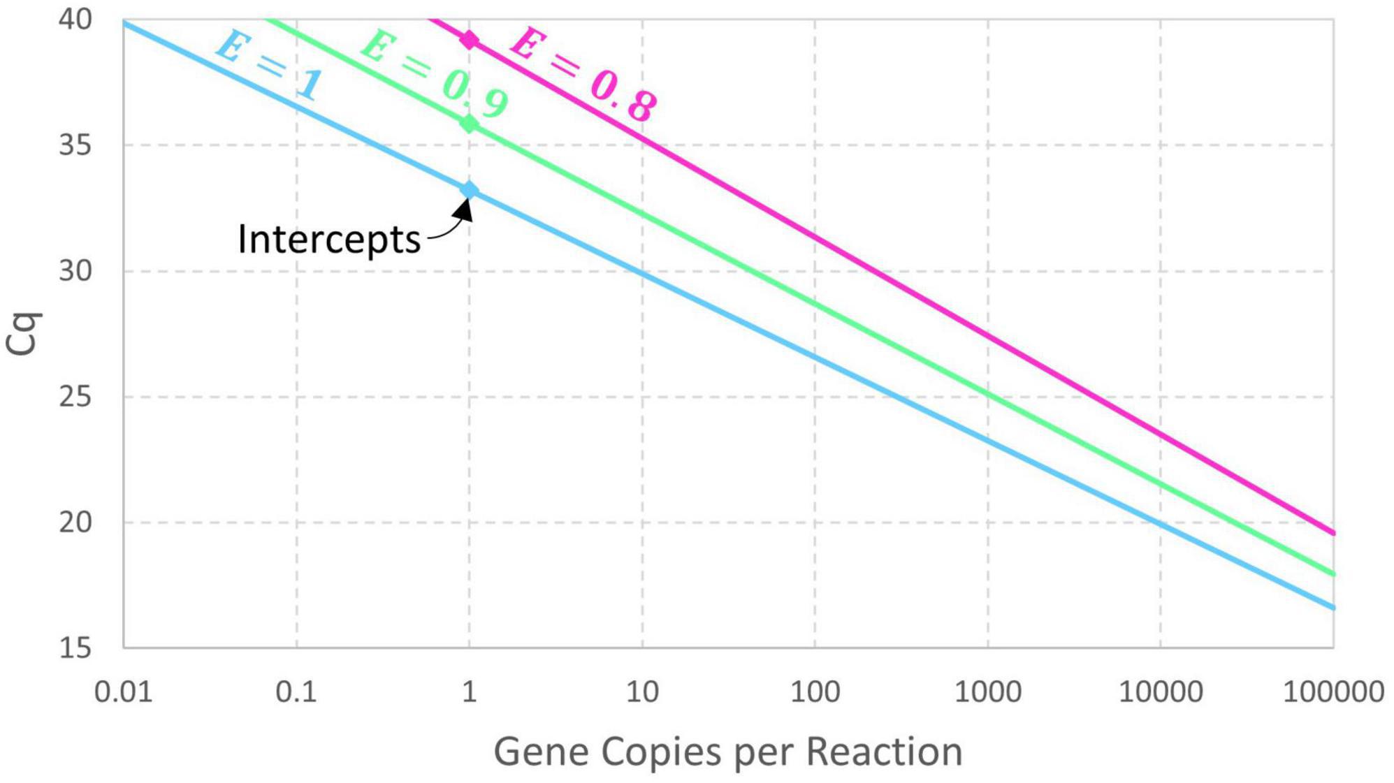
Figure 1. Deterministic log-linear standard curve model with amplicon detection threshold N_q = 10¹⁰ and amplification efficiency E having values of 1, 0.9, and 0.8. The corresponding intercept values are 33.22, 35.87, and 39.17, respectively.

Although amplification efficiency is known to wane eventually, leading to the plateauing of qPCR fluorescence curves, the persistence of exponential growth until the threshold has been disputed (Rutledge and Stewart, 2008b). However, this assumption is not strictly necessary for the above model and less restrictive mechanistic criteria may be described. Separation of Cq values must be established by initial exponential growth persisting until the number of amplicons is greater than the largest tested initial number of target genes (N₀). If this is not the case, waning amplification efficiency will lead to reduced separation of Cq values at high concentrations and an upper limit on the linear dynamic range. At higher numbers of amplicons, the separation in Cq values established by exponential amplification is retained so long as all curves have the same shape—even if waning amplification efficiency leads to sub-exponential amplification. The fluorescence threshold can be set within this sub-exponential region, but not so high that divergence toward reaction-specific plateaus affects the separation of Cq values. Within this region, Cq is not necessarily the number of cycles of exponential growth needed to get to the threshold; the intercept behaves as a tuning parameter to quantify the number of cycles required to amplify a single target gene to the fluorescence threshold whether all of those cycles featured exponential amplification or not.

2.2. Log-linear regression modeling of Cq

The need to analyze standard curve data using a probabilistic approach rather than a deterministic one is exemplified by variation in Cq values among replicates at a particular standard concentration. Log-linear regression is widely used and supported by the log-linear deterministic model in the section “2.1. Deterministic modeling of Cq,” but random scatter in Cq values about the fitted line and its implications are rarely addressed. This section emphasizes potential mechanisms and modeling of this variation. Presuming that the initial number of target genes (N₀) is known and that amplification proceeds deterministically until Cq, error can arise from how Cq is determined from fluorescence data or from well-to-well variation in amplification efficiency. Determination of Cq from fluorescence data involves evaluating background fluorescence for each well and potentially each cycle and using relative fluorescence measurements to represent the portion of the fluorescence attributed to amplifying target genes. Normalization may also be used to correct for well-to-well variation in the capacity to detect fluorescence. Any imprecision in individual fluorescence readings or how they are adjusted would affect the precision of the relative fluorescence readings between which Cq is interpolated. Variation in amplification efficiency could contribute to scatter in Cq values because reactions with lower amplification efficiency would take longer to reach the threshold. However, the effect could diminish at higher concentrations as less amplification is needed to reach the threshold. These errors are mechanistically described as “Cq residual error” because deviations from a fitted regression model are called residuals.

If the error in determining Cq for each well is normally distributed with mean zero and standard deviation σ (called “Cq residual standard deviation” herein), then the result is the conventional log-linear regression model often used in standard curve fitting together with mechanistic interpretation of the random error component. Specifically, Eq. 4 builds probabilistically upon Eq. 3 using N(μ,σ²) notation for a normal distribution with mean μ and variance σ². This model carries on with constant variance σ² to values of N₀ much less than 1 target gene per reaction and cannot explain non-detects that do not yield Cq values at all.

$Cq\sim N(Intercept+Slope\times {\log }_{10}{N}_0,{\mathrm{\sigma }}^2)(4)$

2.3. Incorporating Poisson variation into qPCR data analysis

The log-linear regression standard curve model (Eq. 4) relates Cq to an integer initial number of target genes (N₀) rather than a standard concentration λ. The discordance in contemporary qPCR theory associated with assuming N₀ = λ has diminishing effect at high concentrations, which is why conventional log-linear regression works well in a linear dynamic range but not at low concentrations. At low concentrations, random variation (random sampling error) in the number of discrete objects in an aliquot of known volume from a source of known concentration becomes important. Assuming that volume is carefully controlled, that standards are precisely quantified and diluted, and that target genes are randomly dispersed in these standards, this variation should follow a Poisson distribution (Eq. 5). This error is denoted herein as “reaction random sampling error” because it applies to the initial number of target genes in a PCR reaction. A separate form of random sampling error describing variation in the integer number of instances of the target gene contained in a sample collected from the environment (e.g., prior to processing and extraction) is outside the scope of this work.

$N_0\sim Poisson\left(\mathrm{\lambda }\right)(5)$

This variation is sometimes acknowledged in qPCR data analysis literature, but it is generally not reflected in approaches to standard curve fitting. The weighted regression approach of Tellinghuisen and Spiess (2019) suppresses excess variation at low standard concentrations due to this error but does not account for non-detects (N₀ = 0) that cannot yield Cq values and therefore cause the function Cq = a + b×log⁡N₀ to not have a variance with which to assign weights. Their variance formula is accurate for concentrations at which non-detects are improbable (e.g., >7 gc/rxn) if a zero-truncated Poisson distribution is assumed, but it misrepresents the effect of Poisson variation at lower concentrations. Rather than using the idea of Poisson-distributed N₀ to develop a patch to least squares regression, this research formally conditions a probabilistic regression model (Eq. 4) on Poisson-distributed N₀ (Eq. 5) using hierarchical probabilistic modeling. Addressing the discrete nature of genes as well as the Poisson-distributed variation in the initial number of target genes contained in an aliquot of diluted standard leads to an enhanced standard curve model. All random errors that pertain to preparation of environmental samples for qPCR but not to standard curve experiments using standards with extracted or synthetic genes are outside the scope of this work. This model reflects non-detects (Cq = ND) arising from an N₀ of zero but not from amplification failures or running an insufficient number of cycles.

Figure 2 contrasts 95% probability intervals of Cq (conditional on detection) as a function of continuous concentrations of gene copies per reaction (gc/rxn) with and without reaction random sampling error. The contemporary log-linear regression standard curve model goes off to concentrations below 1 gc/rxn with homogeneous variance and cannot explain non-detects. Reaction random sampling error, on the other hand, leads to (1) increased variability of Cq values at lower concentrations, (2) wells initially containing zero target genes that cannot yield Cq values and are therefore non-detects, and (3) Cq values not being able to greatly exceed the intercept. The effect of this random sampling error appears below 30 gc/rxn in this example, but it would be evident at higher concentrations with smaller values of Cq residual standard deviation σ. With equal numbers of technical replicates at each tested concentration, non-detects lead to progressive sparsity of numeric data below about 3 gc/rxn. Cq values cannot greatly exceed the intercept because N₀ = 1 is the smallest non-zero initial number of target genes.

FIGURE 2

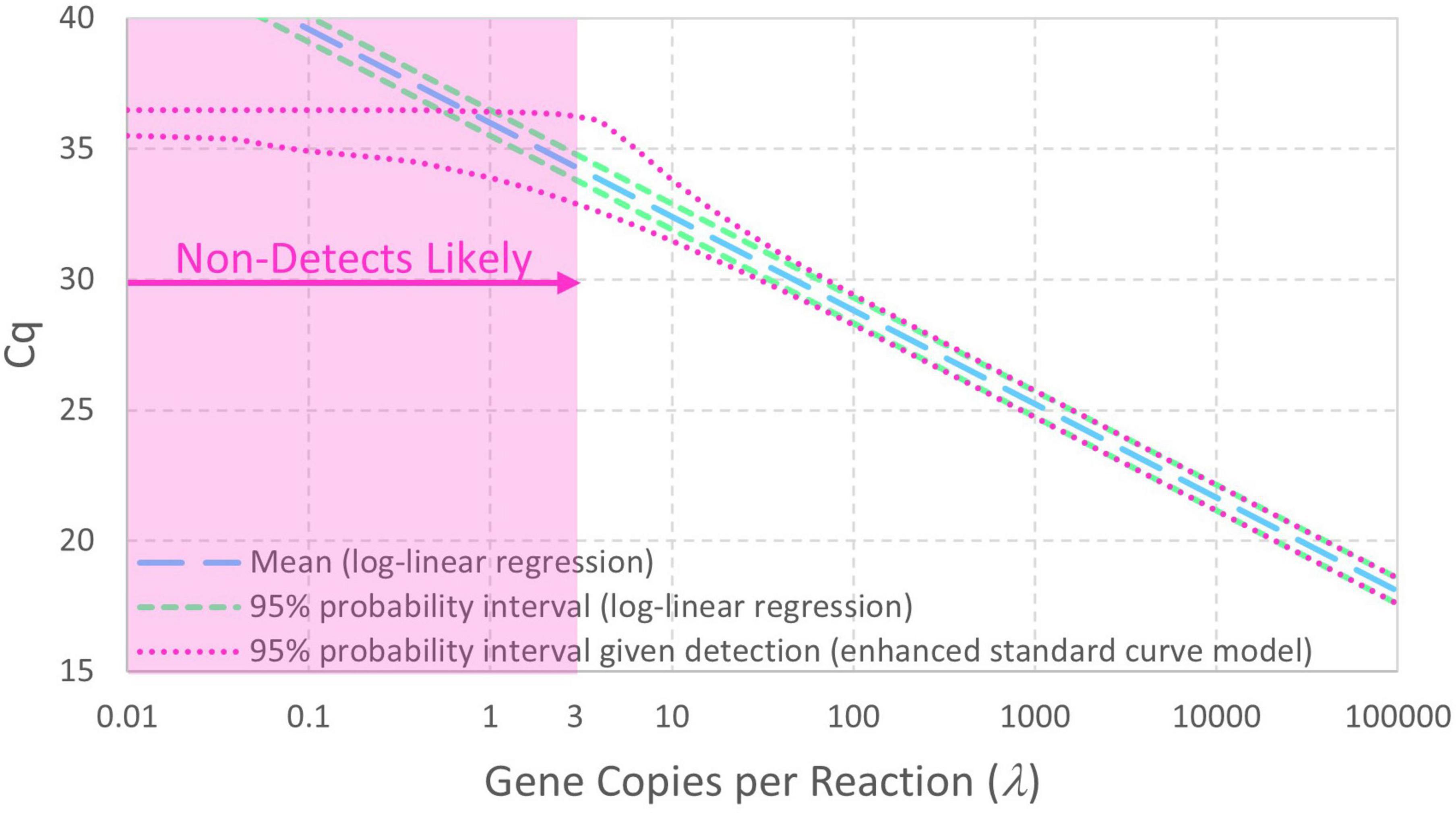
Figure 2. Comparison of standard curve models with and without Poisson-distributed reaction random sampling error given intercept 36, amplification efficiency E = 0.9, and Cq residual standard deviation σ = 0.25. Non-detects are illustrated as likely below 3 gc/rxn, and the 95% probability interval for the enhanced standard curve model (with reaction random sampling error) is conditional on detection.

The enhanced standard curve model combining Eqs. 4, 5 facilitates analysis of standard curve data without arbitrary decisions about which Cq values arising from low standard concentrations should be included in standard curve model fitting. It also facilitates simulation of standard curve data (section “3.1. Simulation of standard curve data”), straightforward evaluation of probabilities and parameter estimates (section “3.2. Numerical integration to compute probability intervals or maximum likelihood estimates”), and evaluation of uncertainty in fitted standard curve model parameters (section 3.3. Parametric uncertainty analysis of standard curve parameters”). In addition to enabling computation of the variability in Cq given a standard concentration λ (in gc/rxn), this model is a first step toward evaluating the uncertainty in qPCR-based concentration estimates (Figure 3). Notably, this model includes essentially the same parameters as log-linear regression (e.g., intercept, slope, and the largely unreported residual standard deviation σ). Usually, increasing the complexity of a model increases the number of parameters and the need for supporting data. No parameters are added in this case because it replaces the assumption that N₀ = λ with a Poisson distribution having only one parameter (λ).

FIGURE 3

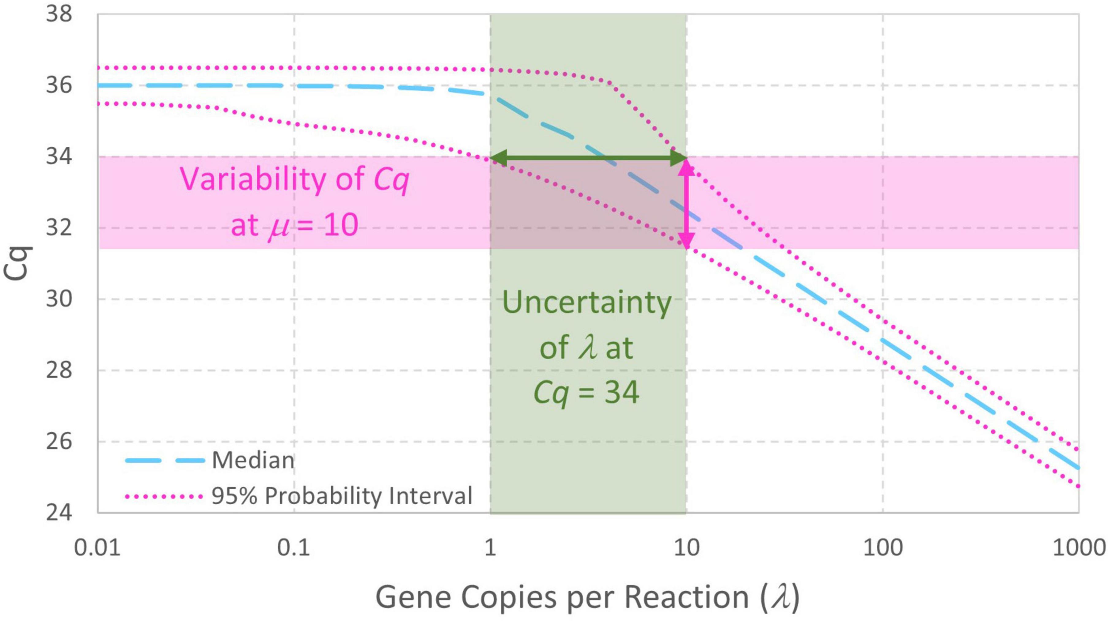
Figure 3. Probability intervals describing variability in Cq as a function of gene copies per reaction also give a visual approximation to begin quantitatively understanding the uncertainty in qPCR-based concentration estimates. The displayed standard curve model includes Poisson-distributed reaction random sampling error and has intercept 36, amplification efficiency E = 0.9, and Cq residual standard deviation σ=0.25.

2.4. Random amplification error

Like the initial number of target genes in a reaction (N₀), the number of amplicons after c PCR cycles (N_c) must also be a non-negative integer. For example, if N₀ = 1 and E = 0.9, then a 1.9-fold increase is expected in each cycle, but it is impossible to have 1.9 amplicons after the first cycle. Instead, there would be a 90% chance of amplifying to two amplicons and a 10% chance of remaining with only one, which yields 1.9 amplicons on average. If this solitary target gene in the well did not amplify in the first cycle, it is as if the first cycle did not exist in terms of advancing toward detection, so Cq is raised by one cycle. The number of amplicons after c cycles may be modeled recursively as a discrete-time Markov chain initialized with N₀ and the transition matrix for cycle c can be populated using Eq. 6. Modeling this “random amplification error” using a binomial distribution presumes that each target gene present either duplicates or fails to duplicate with probability equal to amplification efficiency E that cannot exceed 100%. The resulting value of Cq may then be modeled using Eq. 7 given a value of c corresponding to a large value of N_c that remains within the exponential phase. Addition of this error adds no parameters to the standard curve model because each binomial distribution depends only on the already specified input N_c–1 and amplification efficiency E that was already in the model.

$N_c-N_{c-1}\sim binomial(N_{c-1},E)(6)$

$Cq-c\sim N(Intercept+Slope\times {\log }_{10}{N}_c,{\mathrm{\sigma }}^2)(7)$

Figure 4 provides an illustrative example of random amplification error with N₀ = 1, E = 0.9, and three cycles (because algebraically exploring the effect of random amplification error with numbers of cycles typical of qPCR is intractable). The mean number of amplicons after three cycles is 6.859 (i.e., 1.9³) as expected, but there is substantial random variation. There is a 47.8% chance that there will be 8 amplicons after three cycles and a 1% chance that there will only be two amplicons. The difference between these outcomes in terms of Cq is 2.16 because 2 × 1.9^2.16 = 8. Random amplification error diminishes as the initial number of target genes or number of amplicons increases, meaning that it becomes trivial for larger values of N₀ and, in the c^th cycle, for large N_c–1. Thus, its effect on variability in Cq is similar to reaction random sampling error in that it is relatively inconsequential at high concentrations and becomes progressively more important at low concentrations. For example, three cycles with N₀ = 10 and E = 0.9 are likely to yield between 57 and 78 amplicons (not shown), which would have an effect of only 0.49 on the value of Cq. This is related to the diminishing relative standard deviation (RSD) of the binomial distribution in Eq. 6 ($RSD=\sqrt{\left(1-E\right)/\left(N_{c-1}\times E\right)}$) as N_c–1 increases.

FIGURE 4

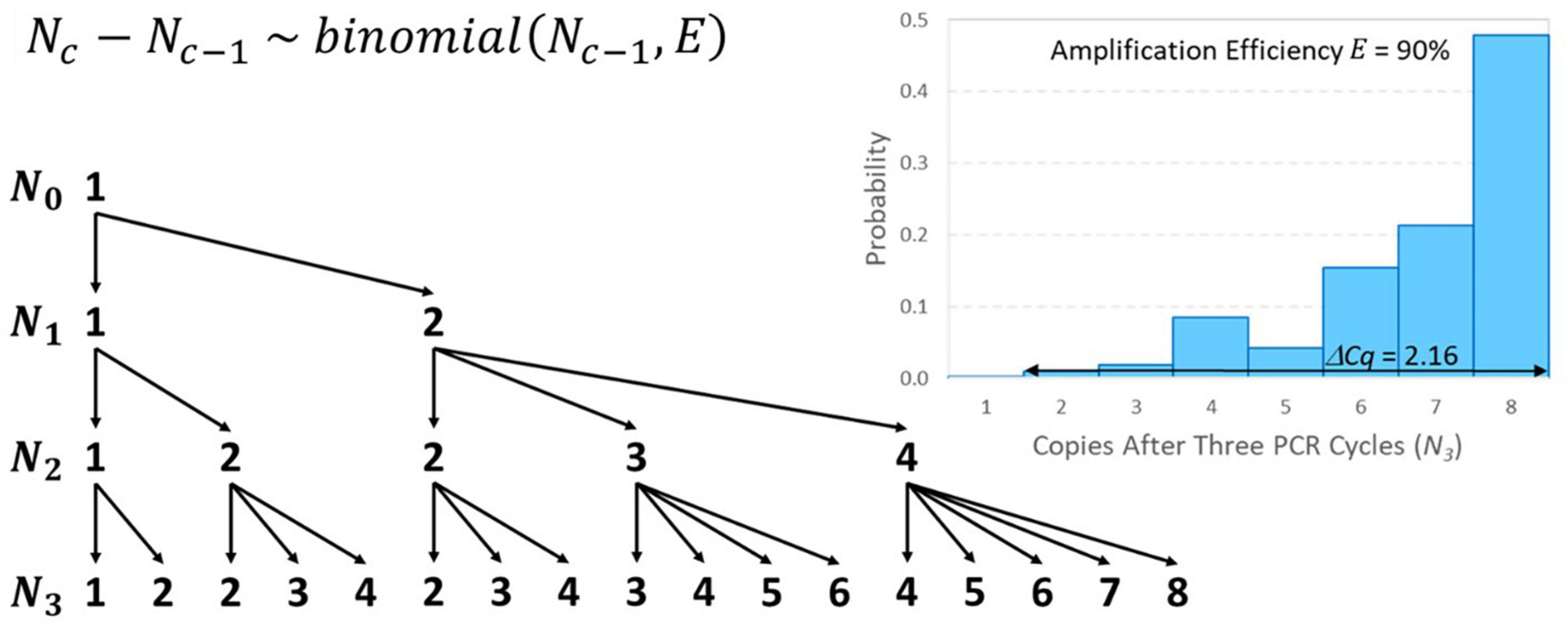
Figure 4. Tree diagram illustrating all possible outcomes of amplifying N₀ = 1 target gene through three PCR cycles and a distribution of resulting numbers of amplicons after three cycles with E = 90% amplification efficiency. The conditional probability associated with each arrow may be calculated using the binomial distribution shown. In terms of 1.9-fold amplification, the difference between having 2 or 8 amplicons after three cycles is 2.16 Cq on average.

2.5. Additional random errors affecting standard curve data

The foregoing development of an enhanced standard curve model and its ensuing application are grounded in the assumption that N₀∼Poisson(λ) and that λ is precisely known. Specifically, it focuses on modeling the relationship between Cq and the nominal concentration of gene copies per reaction (λ) but does not address the accuracy of λ or validity of the Poisson distribution describing random sampling error in wells. Noting that assumptions and limitations are central to model development, additional error mechanisms that are not modeled herein are described below.

There are many mechanisms through which λ may be imprecisely known, including (1) error in the nominal concentration of the undiluted standard, (2) volumetric error in the dilution series, and (3) losses in the dilution series. All of these errors lead to biased concentration estimates. If the concentration of the undiluted standard is higher than indicated, Cq would be reduced and non-detects would be less common than anticipated at nominal concentrations near and below 1 gc/rxn. Conversely, if the concentration of the undiluted standard is lower than indicated, Cq would be increased and non-detects may become unexpectedly common at nominal concentrations near and above 1 gc/rxn. Systematic dilution errors would lead to a compounding error that makes the nominal concentration of more diluted standards more inaccurate (e.g., if a nominal 2-fold dilution is actually a 1.9-fold or 2.1-fold dilution). Consistent losses among dilutions (e.g., due to microorganisms or target genes not successfully discharged from the pipette tip) would also lead to a compounding error akin to dilution error. For example, a 2-fold dilution with 2% losses is effectively a 2.04-fold dilution (2/0.98). Over-dilution and losses will lead to nominal concentrations that are over-stated, increase Cq values, decrease amplification efficiency estimates, and lead to unexpectedly common non-detects near and above 1 gc/rxn. Conversely, under-dilution leads to nominal concentrations that are under-stated, decreases Cq values, increases amplification efficiency estimates, and leads to unexpectedly rare non-detects near and below 1 gc/rxn. It is therefore important to regularly ensure accurate calibration of pipettes to prevent biased estimation of PCR efficiency and associated quantification of target genes arising from insufficiently controlled standard curve data. Unknowingly using an inadequately calibrated pipette or misusing a pipette functionally calibrates qPCR to improperly quantified standards so that both absolute and relative quantification would be biased.

The assumption of a Poisson distribution for well-random sampling error (Eq. 5) is firmly grounded in theory (Student, 1907), but extraneous sources of variation can lead to over-dispersion (Schmidt et al., 2014). These can include spatial heterogeneity in the standard (poor mixing) or non-constant losses or volumetric error in the transfer to the well. A final potential cause of over-dispersion would be clustering of target genes. Target genes that are bound in groups within an otherwise homogeneous and accurately quantified source (i.e., not just having spatially varying concentration due to poor mixing) are known to invalidate the Poisson assumption. This can inflate variability in N₀ relative to a Poisson model, thus increasing the variability in Cq values and increasing the probability of non-detects at specific concentrations. In the analogous context of dose–response models (Schmidt, 2015) in which doses are assumed to be accurately quantified and aggregates are assumed to break up following consumption, clustering would create an illusion that a pathogen is less infectious than it really is by reducing the probability of infection for specific doses. This issue could compromise quantitative reliability of digital PCR because MPN calculations used to interpret arrays of presence–absence results are usually predicated on a Poisson model. Presuming that these issues can be adequately addressed in well-controlled standard curve experiments, modeling of over-dispersion with respect to the Poisson distribution is outside the scope of this work.

3. Methods for using the developed probabilistic models in simulation and model-fitting

Following the model development discussion in the section “2. Describing and modeling random errors in qPCR standard curve data” that focused on representing the foundational theory of standard curve modeling and adapting it to reflect physically meaningful random error mechanisms, this section addresses the more mathematical topic of how to use these models. Tasks addressed include simulation of standard curve data, computation of probability intervals, model fitting using maximum likelihood estimation, and Bayesian methods to evaluate parameter uncertainty.

3.1. Simulation of standard curve data

In mechanistically derived models, Monte Carlo simulation can be useful to explore the anticipated effects of various error mechanisms or to contrast alternative experimental designs or data analysis approaches. The models developed in the section “2. Describing and modeling random errors in qPCR standard curve data” can be used to simulate Cq values given values of model parameters Intercept, E, and σ as well as concentration λ. A custom function in R (R Core Team, 2020) with which data can be simulated is provided in the Supplementary content along with an illustrative example of its use.

3.2. Numerical integration to compute probability intervals or maximum likelihood estimates

To compute probability intervals graphically illustrating variability in Cq values or fit model parameters to available data using maximum likelihood estimation, it is necessary to algebraically characterize the distribution of Cq. Reflecting reaction random sampling error in the log-linear regression model adds complexity to evaluation of the distribution of Cq. Specifically, the model becomes hierarchical because Eq. 4 is conditional on a value of N₀ that is also random according to Eq. 5. Computing the unconditional (or marginal) distribution of Cq requires summation of all non-zero values of N₀ and their respective probabilities, which must be done numerically. The resulting probability density function (Eq. 8) describes only the numeric values of Cq while Eq. 9 describes the non-numeric outcome that Cq is undetermined when N₀ = 0, resulting in a non-detect (Cq = ND). The cumulative distribution function (Eq. 10) is calculated using the standard normal cumulative distribution function Φ(.) and has a maximum value of 1−e^−λ due to non-detects. Derivation of these equations is provided in the Supplementary content, as is an R function with which to perform these calculations. Consideration of random amplification error in this study is limited to theoretical development and simulation because numerical integration is intractable.

$f\left(Cq\right)=\sum _{N_0=1}^{\mathrm{\infty }}\frac{e^{-\mathrm{\lambda }}{\mathrm{\lambda }}^{N_0}}{N_0!}\times \frac{1}{\sqrt{2\mathrm{\pi }}\mathrm{\sigma }}\exp \left\{-\frac{{\left[Cq-\left(Intercept+Slope\cdot {\log }_{10}{N}_0\right)\right]}^2}{2{\mathrm{\sigma }}^2}\right\}(8)$

$P(Cq=ND)=P(N_0=0)=e^{-\mathrm{\lambda }}(9)$

$F\left(Cq\right)=\sum _{N_0=1}^{\mathrm{\infty }}\frac{e^{-\mathrm{\lambda }}{\mathrm{\lambda }}^{N_0}}{N_0!}\times \text{Φ}\left(\frac{Cq-\left(Intercept+Slope\cdot {\log }_{10}{N}_0\right)}{\mathrm{\sigma }}\right)(10)$

Equation 10 is useful to compute probability intervals for Cq, particularly if it is made conditional on detection by dividing it by 1−e^−λ. A 95% probability interval such as the ones displayed in Figures 2, 3 can be calculated for each of a range of concentrations by determining the Cq values corresponding to 2.5% and 97.5% cumulative probability. Eq. 8 is useful for maximum likelihood estimation to determine the values of model parameters that maximize the probability of a set of observed data (R scripts are provided in the Supplementary content). Because non-detects arising from reactions containing no target genes depend on concentration λ (Eq. 9) but not on properties of the PCR, they have no effect on estimation of the fitted standard curve model parameters (i.e., they appear only as constants in the likelihood function used for inference of standard curve model parameters). Non-detects may therefore be omitted from standard curve fitting (but not analysis of environmental data) because it is mathematically justifiable to omit them. This differs from just arbitrarily omitting them because they are incompatible with log-linear regression.

3.3. Parametric uncertainty analysis of standard curve parameters

Ideally, science should not be based solely on providing estimates of values inferred from data but should indicate how good the estimates are or what range of other values could be supported by the data. Parametric uncertainty in estimated parameters of probabilistic models may be fully represented using Bayesian Markov chain Monte Carlo (MCMC) and software such as OpenBUGS (3.2.3 rev 1012; Lunn et al., 2000). The Bayesian process merges observed data and subjective beliefs about parameters (represented by prior distributions) to express uncertainty in the values of estimated model parameters in the form of a posterior distribution. Relatively uninformative priors are often used in absence of well supported subjective beliefs so that the posterior distribution is most strongly influenced by the objective information from the data. Because posterior distributions are often difficult to evaluate algebraically, MCMC is used to draw a set of values representing this posterior distribution. The 2.5th and 97.5th percentiles of the generated parameter values can then be used to define a 95% credible interval in which the analyst is entitled to believe that the true value of the parameter is contained with 95% chance. This section details Bayesian analysis of uncertainty in the parameters of the enhanced standard curve model applying MCMC in OpenBUGS (see model code in Supplementary content). Random amplification error was not implemented in OpenBUGS due to limitations in the model specification step that precluded incorporation of Eq. 6.

Analyses performed herein included a log-uniform prior on the amplicon detection threshold (0 < log₁₀⁡N_q < 15), a uniform prior on amplification efficiency (0 < E < 1), a log-uniform prior on the Cq residual standard deviation (−5 < log₂⁡σ < 1). The upper bound for N_q of 10¹⁵ corresponds to approximately 50 two-fold amplifications of a single target gene. This relatively uninformative prior favors smaller values of N_q but corresponds to a uniform prior on the intercept (conditional on a particular value of amplification efficiency E). Restricting amplification efficiency to E < 1 reflects that it is not theoretically possible to amplify a single target gene more than once in a single PCR cycle and is otherwise relatively uninformative. This prior can have a substantial effect on estimation of E when conventional log-linear regression would give an estimate near or above 100%. Dilution errors (too little diluent and/or pipetting excess standard) and inhibition at high concentrations are known mechanisms for amplification efficiency estimates exceeding 100%. The prior on Cq residual standard deviation (σ) slightly favors smaller values, but it is wide enough to be relatively uninformative in most cases. Cq values typically vary to some extent at high concentrations and a standard deviation of Cq values below 0.5 has been proposed as a performance criterion (Ministry of the Environment, Conservation and Parks [MECP], 2021). Default updating algorithms were used with a burn-in of 10,000 iterations and thinning to every 100th of the next 100,000 iterations to ensure that the generated sample provided a good representation of the posterior distribution. History plots indicated rapid convergence and excellent mixing, and each analysis took about 2 min.

4. Application of model to analysis of simulated standard curve data

For illustrative purposes, an analysis was carried out with 101 data simulated (i.e., randomly generated using the developed models) using concentrations that are equally spaced in logarithmic scale between 0.01 and 1000 gc/rxn (Supplementary Table 1). Simulation of realistic dilutions with many technical replicates at each dilution has less illustrative value because of overlapping points in plots. Data were simulated both with and without random amplification error using an intercept of 36, amplification efficiency E = 0.90, and Cq residual standard deviation σ=0.25. The same Poisson-distributed values of N₀ and normally distributed Cq residual error were used in each scenario so that results differ only in the inclusion or exclusion of random amplification error. The purpose of this simulation experiment was to (1) illustrate the effect of random amplification error relative to only reaction random sampling error and (2) compare alternative model fitting techniques.

Figure 5A shows the data simulated without random amplification error (with non-detects plotted as Cq = ND to allow their illustration). Figure 5B likewise shows the data simulated with random amplification error. Both figures show the 95% probability interval for Cq conditional on detection computed using the model without random amplification error. The similarity of the two graphs shows the subtlety of random amplification error relative to reaction random sampling error, with differences almost imperceptible above 10 gc/rxn. By chance, only one observation falls outside the 95% probability interval in each figure, which is not a particularly improbable result for 67 detections. In Figure 5B, however, the simulated Cq value at 1.58 gc/rxn (circled) is well above the upper bound of the probability interval. This datum had N₀ = 1, and non-amplification of a solitary target gene in the first cycle is known to raise Cq substantially. The probability of such a high Cq value given only reaction random sampling error is < 0.001.

FIGURE 5

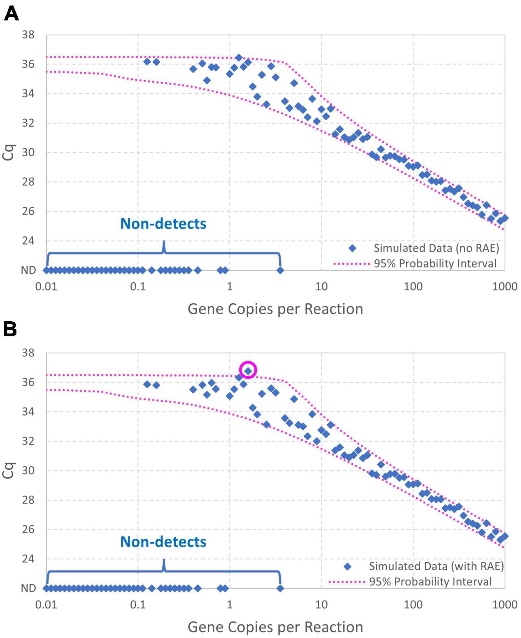
Figure 5. Data simulated (A) with and (B) without random amplification error (RAE). Data were generated using intercept 36, amplification efficiency E = 0.9, and Cq residual standard deviation σ=0.25, and the 95% probability interval was calculated using the same model without including random amplification error. An extreme Cq value highlighting effects of random amplification error is circled.

Three alternative parameter estimation approaches were applied to each simulated dataset for illustrative purposes, with results summarized in Table 1. These included (1) log-linear regression with all obtained Cq values, (2) log-linear regression with only obtained Cq values at concentrations above the highest concentration with a non-detect, and (3) maximum likelihood estimation using the enhanced standard curve model (which does not reflect random amplification error).

TABLE 1

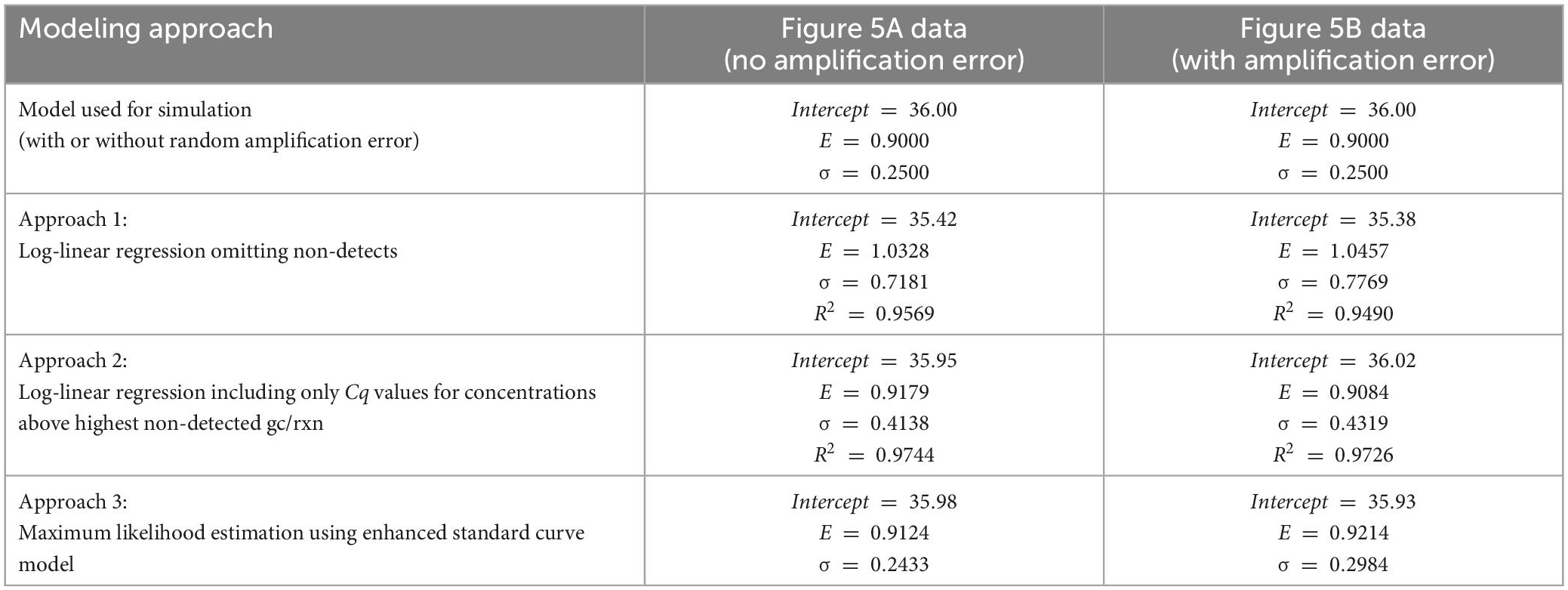
Table 1. Comparison of estimates of the intercept, amplification efficiency (E) and Cq residual standard deviation (σ) using alternative model fitting approaches and data simulated with and without random amplification error.

Critically, when log-linear regression was fit to all Cq data with non-detects omitted (approach 1), the intercept was under-estimated and both the amplification efficiency and Cq residual standard deviation were substantially over-estimated. Applying log-linear regression to Cq values at inappropriately low concentrations can lead to amplification efficiency estimates >100% as shown. This result was anticipated because the regression is being applied to data including Cq values at concentrations below 1 gc/rxn that depart markedly from the log-linear trend. One approach to eliminate this effect is to only apply log-linear regression to Cq values from dilutions with concentrations above the highest concentration at which a non-detect was obtained (approach 2). This approach yields more appropriate intercept and amplification efficiency estimates by excluding any non-linearity, but the Cq residual standard deviation is still over-estimated because log-linear regression cannot explain increasingly variable Cq values as the concentration nears 1 gc/rxn. Values of the coefficient of determination (R²) are shown for the regression methods, as recommended (Bustin et al., 2009). The Cq residual standard deviation (σ) quantifies the consistency of Cq values obtained at high concentrations, while R² quantifies the linearity of the collection of data. Notably, R² can be a misleading performance metric when comparing standard curves with different ranges of tested concentrations: a wider range with poorer consistency of Cq values may yield a higher R² value than a narrower range with better consistency of Cq values.

Logically, maximum likelihood estimation with the enhanced standard curve model (approach 3) yields some of the best parameter estimates because it applies the model used to simulate the data in reverse (except for exclusion of random amplification error). Reversibility is a key feature of probabilistic models that allows them to be used to simulate data given parameters or estimate parameters given data (Schmidt et al., 2022). This method yields the lowest estimates of Cq residual standard deviation (σ) because it accounts for the excess variation in Cq at low concentrations that is introduced by reaction random sampling error. The maximum likelihood estimates for the Figure 5B data include a higher estimate of the Cq residual standard deviation than for the Figure 5A data, possibly to accommodate the inflated variation in Cq and one particularly high value attributed to random amplification error.

Bayesian Markov chain Monte Carlo was also applied to both simulated datasets. Figure 6 shows a scatterplot of results for amplification efficiency E and Cq residual standard deviation σ because these are the two parameters for which the maximum likelihood estimates differ the most between the datasets with and without random amplification error (Table 1). These results show that the amplification efficiency with which the data were simulated (E = 0.9) is well within the quantified uncertainty for each dataset. There is, however, particular divergence in estimation of the Cq residual standard deviation (σ = 0.25). Analysis of data simulated with random amplification error using a statistical procedure that does not include it leads to over-estimation of σ. However, this approach is less biased than the conventional log-linear regression model (Table 1). Continued work to incorporate random amplification error into data analysis and model fitting may be warranted to resolve this bias.

FIGURE 6

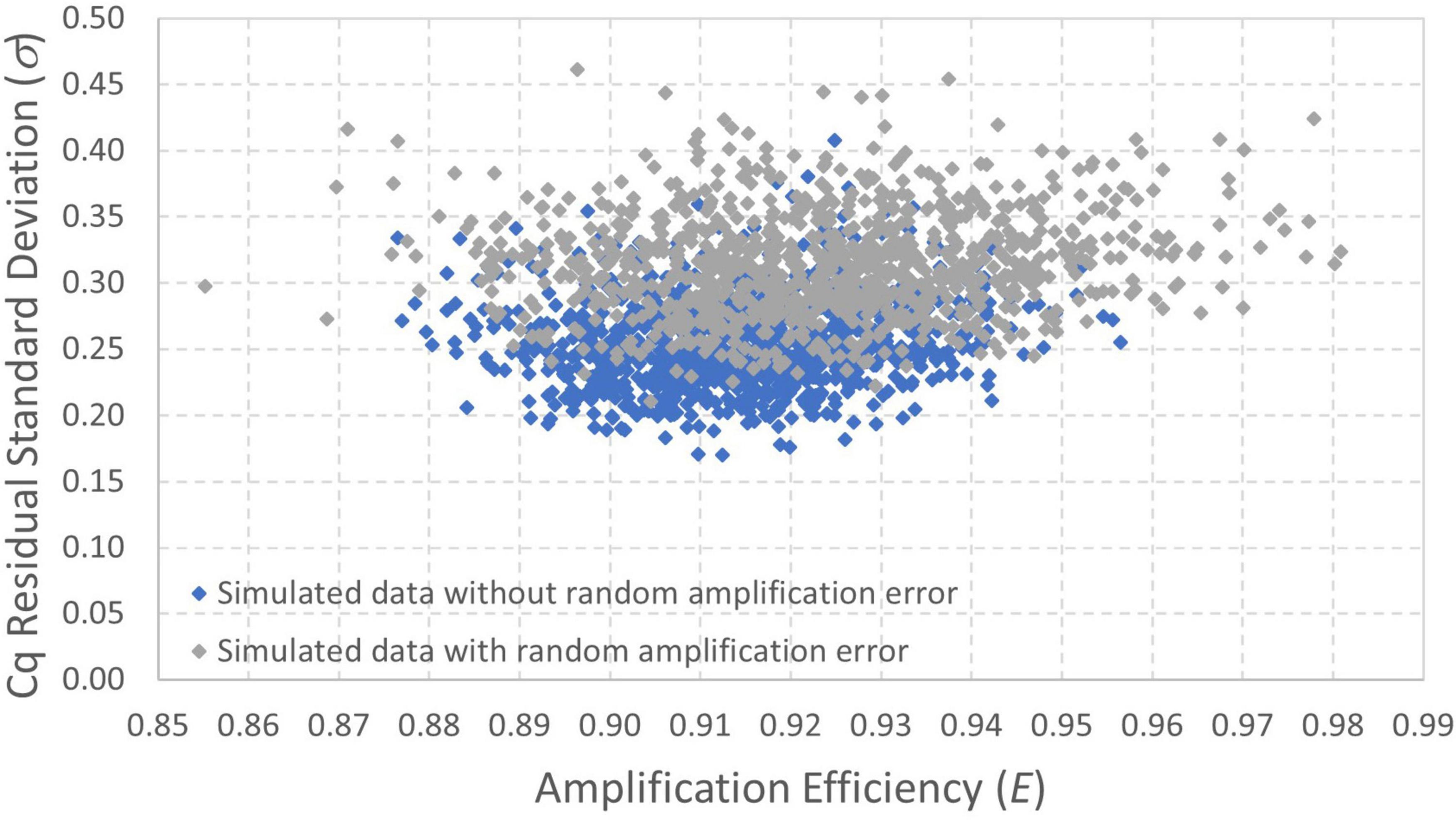
Figure 6. Scatterplot of posterior distributions quantifying uncertainty in amplification efficiency and Cq residual standard deviation estimated from datasets simulated with and without random amplification error (Figures 5A,B, respectively). The data were simulated with E = 0.9 and σ=0.25.

5. Application of model to analysis of experimental standard curve data

Standard curves may be evaluated for two reasons: to evaluate performance metrics such as a limit of detection or limit of quantification or to provide calibration that facilitates estimation of the concentration of samples that were not prepared from standards. Standard curves targeting evaluation of a limit of detection or limit of quantification may include large numbers of technical replicates prepared from dilutions with low concentrations (sometimes below 1 gc/rxn) but do not always include high concentrations. Standard curves prepared for plate-specific calibration may have fewer technical replicates and a wide range of concentrations that may not include concentrations near 1 gc/rxn. To provide a useful illustrative example reflecting both extremes, a standard curve of the N1 region of the SARS-CoV-2 nucleocapsid gene using a standard with synthetic RNA transcripts (#COV019, EDX, USA) was prepared. Specifically, the standard was serially diluted (2x) in 20 ng/μL Poly(A) (#10108626001, Roche, Germany) and TE buffer (#BP2473100, Fisher Scientific, USA) with concentrations ranging from 200 to 0.39 gc/rxn. The assay for the N1 target followed the CDC 2019-nCoV Real-Time RT-PCR Diagnostic Panel (Centers for Disease Control and Prevention [CDC], 2020) with primers and probes purchased from Sigma-Aldrich (USA). TaqPath™ 1-Step RT-qPCR Master Mix, CG (A15299, ThermoFisher, USA) was used. Nine technical replicates for each standard and six no-template controls (NTCs) were plated on a 96-well plate (Supplementary Table 2). qPCR was run on the OPUS system (Bio-Rad, USA) with conditions outlined in Supplementary Table 3. Based on the developed model it was anticipated that there would be (1) low variability in Cq at high concentrations, (2) increasing variability in Cq at low concentrations, (3) non-detects starting to appear near 3 gc/rxn, (4) some Cq values deviating from the log-linear pattern below 1 gc/rxn, and (5) no Cq values more than perhaps 3σ above the intercept.

Figure 7 shows the results of this standard curve experiment as well as the log-linear regression standard curve model fit by the instrument software to all Cq values (omitting only the non-detects). The Cq values at concentrations below 1 gc/rxn do not clearly diverge from the log-linear trend and there are several data that are more than 1 cycle above the intercept of 37.88 obtained using conventional log-linear regression omitting non-detects. Such results may be attributable to the small number of detections at low concentrations and excess variation due to random amplification error. Maximum likelihood estimation was applied to these data using the enhanced standard curve model. The resulting parameter estimates were an intercept of 38.35, amplification efficiency of 0.8593, and Cq residual standard deviation of 0.4363. In contrast, the parameter estimates obtained by log-linear regression with non-detects omitted are 37.88, 0.9476, and 0.5899, respectively. This analysis flagged the datum with Cq = 40.46 as an extreme value (because the modeled probability of a Cq higher than this at 0.78 gc/rxn was <10^–6). Small numbers of wells yielding Cq values that are difficult to explain are not uncommon in practice, and it is desirable to provide a statistical basis for excluding such results in absence of a known error. The analysis was repeated with this value excluded, leading to an estimated intercept of 38.18, amplification efficiency of 0.8906, and Cq residual standard deviation of 0.3072. The latter parameter was particularly affected by excluding the datum in question.

FIGURE 7

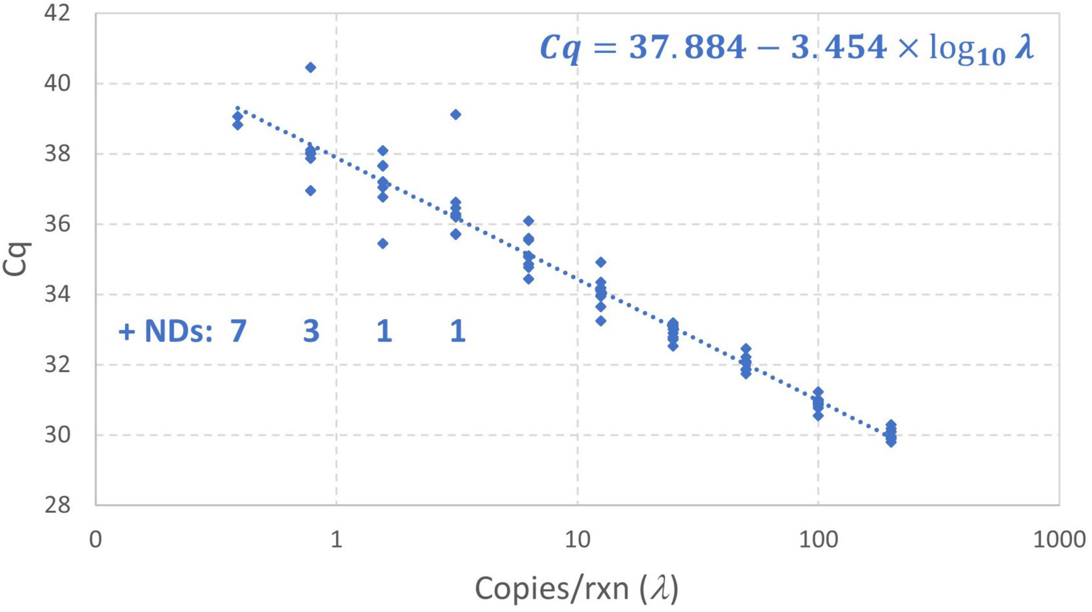
Figure 7. Empirical standard curve data for synthetic N1 target of SARS-CoV-2 using nine technical replicates at each two-fold dilution between 0.39 and 200 gc/rxn. The log-linear regression standard curve model fitted by the instrument software is shown.

Figure 8 includes 95% probability intervals calculated using the maximum likelihood estimates of the model parameters with the one extreme datum excluded. With these probability intervals, it is evident that there are a few somewhat improbable Cq values, but none are so glaring as the one datum that was excluded. Bayesian Markov chain Monte Carlo analysis (not shown) of the data excluding the one high Cq value was carried out to quantify uncertainty in each estimated parameter of the enhanced standard curve model using 95% credible intervals: the results are an intercept of 38.18 (37.95–38.40), amplification efficiency of 89.06% (84.93%–93.79%), and Cq residual standard deviation of 0.3072 (0.2533–0.4038).

FIGURE 8

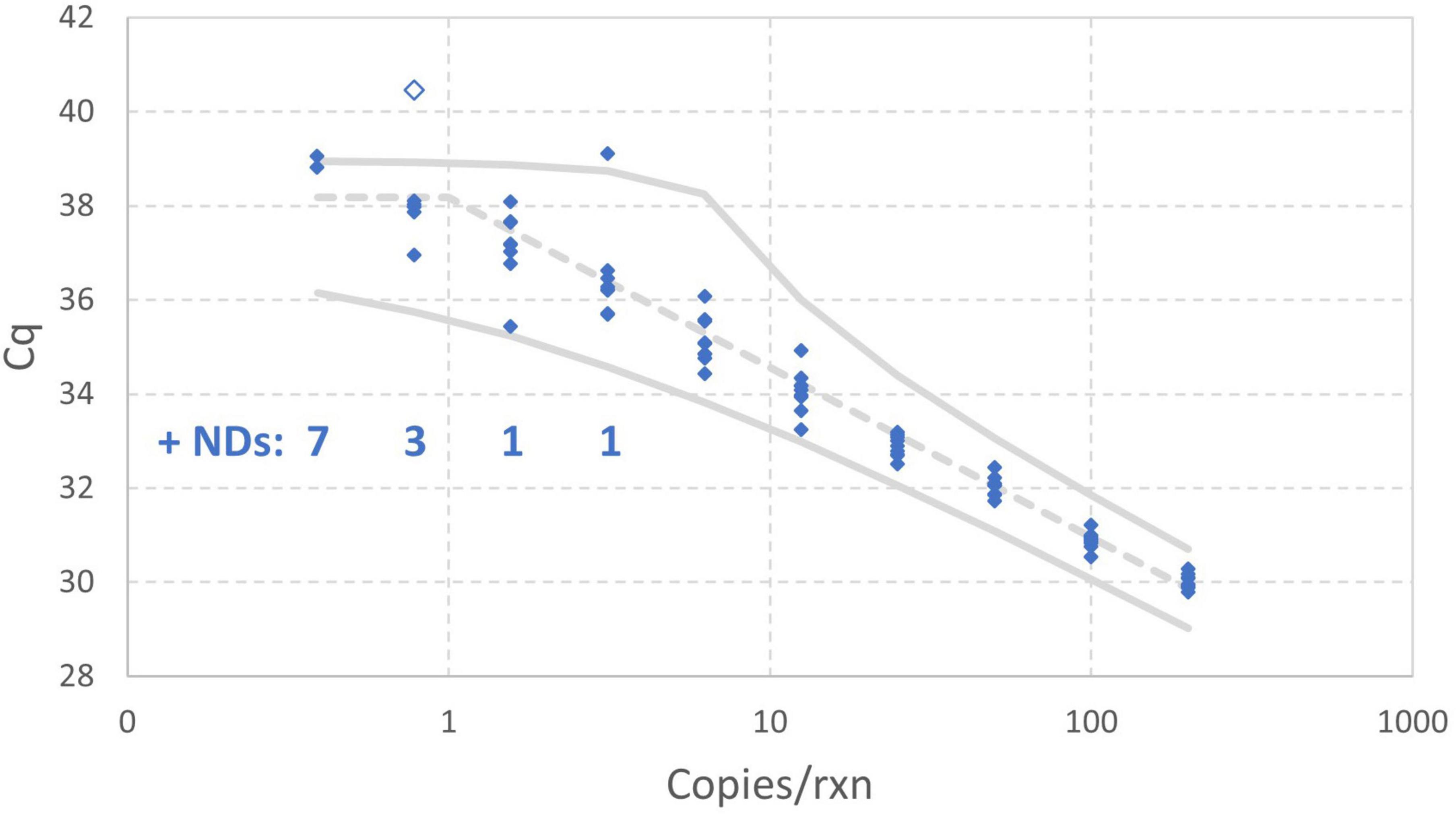
Figure 8. Empirical standard curve data for synthetic N1 target of SARS-CoV-2 using nine technical replicates at each two-fold dilution between 0.39 and 200 gc/rxn. 95% probability intervals (solid gray) and the median (dashed gray) were computed using maximum likelihood estimates for the enhanced standard curve model with one datum excluded as an extreme value.

6. Discussion

Quantitative inference about target gene concentrations via qPCR has often been grounded in log-linear regression to establish a standard curve. This borrows concepts from analytical chemistry, which often depends on linear calibration models to relate observed signals to concentrations of interest. Within a linear dynamic range comprised exclusively of relatively high concentrations that do not generate non-detects or particularly inflated variability in Cq, this approach is dependable. However, conventional standard curve analysis requires exclusion of problematic data at low concentrations (e.g., non-detects and data exhibiting excess variation in Cq or non-linearity) for model fitting. There is also a lack of trust in extrapolation of the standard curve to high Cq values and lack of clarity about handling of non-detects when it is applied to estimate concentrations in environmental samples. In many cases it is easier to dismiss these “non-standard” data than to tackle the statistical problem of inference from data that the log-linear regression model cannot explain. However, scenarios where low concentrations abound and small changes in concentration (e.g., 10% rather than an order of magnitude) are important—such as wastewater-based epidemiology for SARS-CoV-2 (e.g., Chik et al., 2021)—demand advances in standard curve modeling at low concentrations. Such work can aid public health decision-making by helping to determine the sensitivity to detect a meaningful change in concentration on one hand or if an observed change can be explained by random variation alone on the other. This is particularly true in cases where, for whatever reason, digital PCR is not being used and in which explicitly quantifying the uncertainty of qPCR may help data users in their choice of appropriate methodology.

Building on conventional qPCR theory and foundational quantitative microbiology theory involving Poisson processes, this work mechanistically describes the non-linear pattern and increased variability of Cq values observed at low concentrations as well as non-detects. Critically, the developed model is not an empirical model that requires large amounts of data to describe phenomena with more numerous fitted parameters and that may have limited application outside intensely studied case-specific scenarios. The enhanced standard curve model is a mechanistic model developed from theoretical principles that should be no less broadly applicable than the MPN approach to estimating concentrations and adds no case-specific fitting parameters. This model describes why non-detects and changing patterns of Cq values occur at low concentrations, facilitates model fitting without arbitrary decisions about which data to exclude from linear modeling, and enables characterization of the uncertainty in fitted parameters for which only point estimates have typically been provided.

With continued efforts to validate and develop this type of modeling framework (including packaging tools to improve their accessibility to practitioners), this approach can unlock additional value in qPCR-based quantification outside of the linear dynamic range, whether it is applied to estimating gene concentrations in various water matrices or more generally quantifying gene abundances in other contexts. Moreover, it can aid quantification of the uncertainty in all qPCR-based results rather than merely reporting point-estimates mapped from a linear standard curve model. It provides a path forward to improve qPCR data quality by developing guidelines for standard curve experiment design and inter-lab comparison. It also provides a foundation from which to explore additional random errors in qPCR such as losses in the concentration/purification and extraction processes that may depend on matrix effects and a means to extract as much value as possible out of available data. These activities will improve the utility of qPCR to generate epidemiologically meaningful trends in the context of wastewater monitoring of SARS-CoV-2 and other pathogens and to quantify exposures in microbial risk assessments to advance the protection of public health. More generally, it will improve the quantitative value of qPCR beyond detecting order-of-magnitude relative differences.

Data availability statement

The original contributions presented in this study are included in the article/Supplementary material, further inquiries can be directed to the corresponding author.

Author contributions

PS, AC, and ME conceived the need for this work. ME and PS developed the framework for completing this work, secured the funding, and drafted the manuscript. PS conducted the analysis. NA, PD’A, RD, HD, MG, CH, JK, CM, X-LP, SP, NP, YQ, and MS contributed to the data and perspectives regarding laboratory practices. HD and MS conducted the supporting experimental analyses (described in the section “5. Application of model to analysis of experimental standard curve data”). All authors contributed to the article and approved the submitted version.

Funding

We acknowledge the support of Health Canada (2122-HQ-000134), Alberta Innovates (AI 2385B), the City of Calgary (SRA# 088309), the Canada First Research Excellence Fund Global Water Futures program (419205), the Canadian Institutes for Health Research (CIHR; VR5-172693), and the Government of Alberta (Alberta Health; 014562). This research was undertaken, in part, thanks to the Ontario Ministry of Environment, Conservation and Parks Wastewater Surveillance Initiative (MS) and funding from the Canada Research Chairs Program (ME – CRC in Water Science, Technology and Policy; MS – CRC in Water Quality Protection).

Acknowledgments

We are grateful for the discussion of this work with Dr. David Champredon (Public Health Risk Sciences Division, National Microbiology Laboratory, Public Health Agency of Canada) and Prof. William B. Anderson (Department of Civil and Environmental Engineering, University of Waterloo). Additionally, large multi-disciplinary teams across Canada obtained and processed wastewater samples by RT-qPCR to generate data that helped to inform this study and provided helpful context, comments, and questions.

Conflict of interest

The authors declare that the research was conducted in the absence of any commercial or financial relationships that could be construed as a potential conflict of interest.

Publisher’s note

All claims expressed in this article are solely those of the authors and do not necessarily represent those of their affiliated organizations, or those of the publisher, the editors and the reviewers. Any product that may be evaluated in this article, or claim that may be made by its manufacturer, is not guaranteed or endorsed by the publisher.

Supplementary material

The Supplementary Material for this article can be found online at: https://www.frontiersin.org/articles/10.3389/fmicb.2023.1048661/full#supplementary-material

References

Boggy, G. J., and Woolf, P. J. (2010). A mechanistic model of PCR for accurate quantification of quantitative PCR data. PLoS One 5:e12355. doi: 10.1371/journal.pone.0012355

PubMed Abstract | CrossRef Full Text | Google Scholar

Bustin, S. A., Benes, V., Garson, J. A., Hellemans, J., Huggett, J., Kubista, M., et al. (2009). The MIQE guidelines: Minimum information for publication of quantitative real-time PCR experiments. Clin. Chem. 55, 611–622. doi: 10.1373/clinchem.2008.112797

PubMed Abstract | CrossRef Full Text | Google Scholar

Bustin, S. A., Mueller, R., and Nolan, T. (2020). “Parameters for successful PCR primer design,” in Quantitative real-time PCR: Methods and protocols. Methods in molecular biology, Vol. 2065, eds R. Bassioni and A. Raso (New York, NY: Humana). doi: 10.1007/978-1-4939-9833-3_2

PubMed Abstract | CrossRef Full Text | Google Scholar

Centers for Disease Control and Prevention [CDC] (2020). Research use only 2019-novel coronavirus (2019-nCoV) real-time RT-PCR primers and probes. CDC’s diagnostic test for COVID-19 only and supplies, 2019–2020. Available online at: https://www.cdc.gov/coronavirus/2019-ncov/lab/virus-requests.html (accessed November 14, 2022).

Google Scholar

Chik, A. H. S., Glier, M. B., Servos, M., Mangat, C. S., Pang, X.-L., Qiu, Y., et al. (2021). Comparison of approaches to quantify SARS-CoV-2 in wastewater using RT-qPCR: Results and implications from a collaborative inter-laboratory study in Canada. J. Environ. Sci. 107, 218–229. doi: 10.1016/j.jes.2021.01.029

PubMed Abstract | CrossRef Full Text | Google Scholar

Chik, A. H. S., Schmidt, P. J., and Emelko, M. B. (2018). Learning something from nothing: The critical importance of rethinking microbial non-detects. Front. Microbiol. 9:2304. doi: 10.3389/fmicb.2018.02304

PubMed Abstract | CrossRef Full Text | Google Scholar

Eisenhart, C., and Wilson, P. W. (1943). Statistical methods and control in bacteriology. Bacteriol. Rev. 7, 57–137. doi: 10.1128/br.7.2.57-137.1943

PubMed Abstract | CrossRef Full Text | Google Scholar

Fisher, R. A., Thornton, H. G., and Mackenzie, W. A. (1922). The accuracy of the plating method of estimating the density of bacterial populations. Ann. Appl. Biol. 9, 325–359. doi: 10.1111/j.1744-7348.1922.tb05962.x

CrossRef Full Text | Google Scholar

Forootan, A., Sjöback, R., Björkman, J., Sjögreen, B., Linz, L., and Kubista, M. (2017). Methods to determine limit of detection and limit of quantification in quantitative real-time PCR (qPCR). Biomol. Detect. Quantif. 12, 1–6. doi: 10.1016/j.bdq.2017.04.001

PubMed Abstract | CrossRef Full Text | Google Scholar

Gawlik, B. M., Tavazzi, S., Mariani, G., Skejo, H., Sponar, M., Higgins, T., et al. (2021). SARS-CoV-2 surveillance employing sewage: Towards a sentinel system. Technical report. Maastricht: European Union. doi: 10.2760/300580

CrossRef Full Text | Google Scholar

Helsel, D. R. (2006). Fabricating data: How substituting values for nondetects can ruin results, and what can be done about it. Chemosphere 65, 2434–2439. doi: 10.1016/j.chemosphere.2006.04.051

PubMed Abstract | CrossRef Full Text | Google Scholar

Karrer, E. E., Lincoln, J. E., Hogenhout, S., Bennett, A. B., Bostock, R. M., Martineau, B., et al. (1995). In situ isolation of mRNA from individual plant cells: Creation of cell-specific cDNA libraries. Proc. Natl. Acad. Sci. U.S.A. 92, 3814–3818. doi: 10.1073/pnas.92.9.3814

PubMed Abstract | CrossRef Full Text | Google Scholar

Lunn, D. J., Thomas, A., Best, N., and Spiegelhalter, D. (2000). WinBUGS - A Bayesian modelling framework: Concepts, structure, and extensibility. Stat. Comp. 10, 325–337. doi: 10.1023/A:1008929526011

CrossRef Full Text | Google Scholar

McCall, M. N., McMurray, H. R., Land, H., and Almudevar, A. (2014). On non-detects in qPCR data. Bioinformatics 30, 2310–2316. doi: 10.1093/bioinformatics/btu239

PubMed Abstract | CrossRef Full Text | Google Scholar

McCrady, M. H. (1915). The numerical interpretation of fermentation-tube results. J. Infect. Dis. 17, 183–212. doi: 10.1093/infdis/17.1.183

CrossRef Full Text | Google Scholar

Ministry of the Environment, Conservation and Parks [MECP]. (2021). Protocol for evaluations of RT-qPCR performance characteristics: Technical guidance. Toronto, ON: Ministry of the Environment, Conservation and Parks (MECP), doi: 10.13140/RG.2.2.10627.02080

CrossRef Full Text | Google Scholar

Nahrstedt, A., and Gimbel, R. (1996). A statistical method for determining the reliability of the analytical results in the detection of Cryptosporidium and Giardia in water. J. Water Supply Res. Technol. 45, 101–111.

Google Scholar

Quan, P.-L., Sauzade, M., and Brouzes, E. (2018). dPCR: A technology review. Sensors 18:1271. doi: 10.3390/s18041271

PubMed Abstract | CrossRef Full Text | Google Scholar

R Core Team (2020). R: A language and environment for statistical computing. Vienna: R Foundation for Statistical Computing.

Google Scholar

Ruijter, J. M., Pfaffl, M. W., Zhao, S., Spiess, A. N., Boggy, G., Blom, J., et al. (2013). Evaluation of qPCR curve analysis methods for reliable biomarker discovery: Bias, resolution, precision, and implications. Methods 59, 32–46. doi: 10.1016/j.ymeth.2012.08.011

PubMed Abstract | CrossRef Full Text | Google Scholar

Ruijter, J. M., Ramakers, C., Hoogaars, W. M. H., Karlen, Y., Bakker, O., Van den Hoff, M. J. B., et al. (2009). Amplification efficiency: Linking baseline and bias in the analysis of quantitative PCR data. Nucleic Acids Res. 37:e45. doi: 10.1093/nar/gkp045

PubMed Abstract | CrossRef Full Text | Google Scholar

Rutledge, R. G., and Côté, C. (2003). Mathematics of quantitative kinetic PCR and the application of standard curves. Nucleic Acids Res. 31:e93. doi: 10.1093/nar/gng093

PubMed Abstract | CrossRef Full Text | Google Scholar

Rutledge, R. G., and Stewart, D. (2008a). A kinetic-based sigmoidal model for the polymerase chain reaction and its application to high-capacity absolute quantitative real-time PCR. BMC Biotechnol. 8:47. doi: 10.1186/1472-6750-8-47

PubMed Abstract | CrossRef Full Text | Google Scholar

Rutledge, R. G., and Stewart, D. (2008b). Critical evaluation of methods used to determine amplification efficiency refutes the exponential character of real-time PCR. BMC Mol. Biol. 9:96. doi: 10.1186/1471-2199-9-96

PubMed Abstract | CrossRef Full Text | Google Scholar

Schmidt, P. J. (2015). Norovirus dose-response: Are currently available data informative enough to determine how susceptible humans are to infection from a single virus? Risk Anal. 35, 1364–1383. doi: 10.1111/risa.12323

PubMed Abstract | CrossRef Full Text | Google Scholar

Schmidt, P. J., Cameron, E. S., Müller, K. M., and Emelko, M. B. (2022). Ensuring that fundamentals of quantitative microbiology are reflected in microbial diversity analyses based on next-generation sequencing. Front. Microbiol. 13:728146. doi: 10.3389/fmicb.2022.728146

PubMed Abstract | CrossRef Full Text | Google Scholar

Schmidt, P. J., Emelko, M. B., and Thompson, M. E. (2014). Variance decomposition: A tool enabling strategic improvement of the precision of analytical recovery and concentration estimates associated with microorganism enumeration methods. Water Res. 55, 203–214. doi: 10.1016/j.watres.2014.02.015

PubMed Abstract | CrossRef Full Text | Google Scholar

Student. (1907). On the error of counting with a haemacytometer. Biometrika 5, 351–360. doi: 10.2307/2331633

CrossRef Full Text | Google Scholar

Svec, D., Tichopad, A., Novosadova, V., Pfaffl, M. W., and Kubista, M. (2015). How good is a PCR efficiency estimate: Recommendations for precise and robust qPCR efficiency assessments. Biomol. Detect. Quant. 3, 9–16. doi: 10.1016/j.bdq.2015.01.005

PubMed Abstract | CrossRef Full Text | Google Scholar

Tellinghuisen, J., and Spiess, A. N. (2014). Statistical uncertainty and its propagation in the analysis of quantitative polymerase chain reaction data: Comparison of methods. Anal. Biochem. 464, 94–102. doi: 10.1016/j.ab.2014.06.015

PubMed Abstract | CrossRef Full Text | Google Scholar

Tellinghuisen, J., and Spiess, A. N. (2019). qPCR data analysis: Better results through iconoclasm. Biomol. Detect. Quantif. 17:100084. doi: 10.1016/j.bdq.2019.100084

PubMed Abstract | CrossRef Full Text | Google Scholar