 Christophe Sun1
 David Holcman
- 1Group of Data Modeling, Computational Biology and Predictive Medicine, Institut de Biologie (IBENS), École Normale Supérieure, Université PSL, Paris, France
- 2Département d'Anesthésie-Réanimation, Hôpital Bichat-Claude Bernard, Assistance Publique-Hôpitaux de Paris, Paris, France
- 3Churchill College, Cambridge, United Kingdom
Introduction: Electroencephalography (EEG) signals contain transient oscillation patterns commonly used to classify brain states in responses to action, sleep, coma or anesthesia.
Methods: Using a time-frequency analysis of the EEG, we search for possible causal correlations between the successive phases of general anesthesia. We hypothesize that it could be possible to anticipate recovery patterns from the induction or maintenance phases. For that goal, we track the maximum power of the α−band and follow its time course.
Results and discussion: We quantify the frequency shift of the α−band during the recovery phase and the associated duration. Using Pearson coefficient and Bayes factor, we report non-significant linear correlation between the α−band frequency and duration shifts during recovery and the presence of the δ or the α rhythms during the maintenance phase. We also found no correlations between the α−band emergence trajectory and the total duration of the flat EEG epochs (iso-electric suppressions) induced by a propofol bolus injected during induction. Finally, we quantify the instability of the α−band using the mathematical total variation that measures possible deviations from a flat line. To conclude, the present correlative analysis shows that EEG dynamics extracted from the initial and maintenance phases of general anesthesia cannot anticipate both the emergence trajectory and the extubation time.
1. Introduction
Time-frequency analysis (1, 2) applied to the electroencephalography (EEG) signal has revealed persistent and transient oscillatory bands that are used to classify the brain states (3). Often used to quantify the different oscillatory bands, signal processing parameters include the power spectrum (4), the energy of each band (2), but also the duration of iso-electric suppressions (IES) or α−band suppressions (5), that are segments where the amplitude is below a given threshold. These quantifications benefited from wavelet approaches (6–9) to filter the EEG in real time or to remove noisy perturbations or artifacts (10, 11).
The paradigm shift from EEG correlative and statistical analysis to a predictive approach has relied on the maturation of machine learning approaches (12). Thus, predicting brain sensitivity during general Anesthesia (GA) became possible by quantifying the abundance of IES, markers of a deep sedation or a “vulnerable brain” (13).
These local flat EEG events could be anticipated by the dynamics of α−band suppressions (5), or by combining first passage events, such as the first occurrence time when IES appeared (14). Low frontal α power was also found to be associated with an increase probability of finding IES and Burst-Suppression in the EEG signal (13, 15). These results called for more correlations between the three stages of GA consisting in (1) induction, (2) maintenance, and (3) recovery.
First, the induction phase recapitulates the beginning of hypnotic drug administration, such as propofol or sevoflurane (16–18). These drugs create an artificial and reversible coma preventing brain memorization of surgical events. Induction is the transition period from an awake to a sedative state. The initial hypnotic dosage is often calibrated on patient age and is proportional to the weight (19). This phase lasts from few to around 10 min, as long as necessary to adjust the patient into a stable sedative state. Induction is also associated with a change of the EEG spectral frequency bands with the appearance of a stable α−oscillation in the 8–12 Hz frequency band characterizing this loss of consciousness (LOC). Second, during the maintenance phase, the anesthetic dosage is often adjusted on monitoring machines to maintain the EEG frequencies with the presence of δ and α rhythms during the entire surgical procedure. However, the α−band can sometimes disappear and periods of IES and Burst-Suppression could accumulate over time. It remains an open question to anticipate the brain propensity to generate these EEG instabilities from the induction phase, that could be interpreted as a sign of excessive anesthesia depth. Finally, the recovery phase is associated to the return to consciousness once the anesthetic dosage is gradually cut off. The EEG spectrogram shows a shift toward higher frequency bands (β and γ) and the spectral analysis reveals a stereotype “zip”-shape signature, where the maximum power frequency within the α−band increases during the recovery of consciousness (ROC), while the δ−band decreases until it disappears (20, 21). However, the EEG signal during recovery is not the reversal of the one recorded during induction, as it is controlled by neuronal circuit recovery due to hypnotic elimination, while the time scale of LOC is associated to dominance of cortical inhibitory neuronal synchronization (22–24).
Previous works (5, 14) showed that the statistics of αS during induction correlates with the appearance of IES during maintenance. We explore in the present manuscript, whether other correlations could exist between the three phases of GA. For example, a sensitivity detected during induction could lead to many IES and thus overdosage, leading ultimately to a possible longer time for ROC. Finding further correlations requires to analyze the dynamics of the α−band by computing mathematical indices such as the total variation Vα of the maximum α−oscillations (2). This total variation measures the deviation of α−oscillations maximum amplitude from a flat line. We will develop a fitting procedure for this band and estimate the duration of the α−band emergence trajectory, during which the frequency shifts significantly upwards after the hypnotic injection is stopped. We use these parameters to study the possible correlations between the recovery and the previous phases of anesthesia. We quantify the duration and frequency shifts of the α−band emergence trajectory for the ROC by fitting the power of the α−band with a sigmoid function. Finally, exploring whether there are correlations in the EEG signal between the three phases of GA could be used to anticipate the next phase from the previous ones. We report here mostly weak correlations between the various indices. These results suggest that the sedation depth of the brain should be constantly monitored toward an optimal state: neither too deep nor too light, which remains to be formulated in mathematical terms.
2. Materials and methods
2.1. EEG recordings and preprocessing
EEG monitoring was performed by the Masimo Root® monitor with four frontal electrodes F7, Fp1, Fp2, F8 in the 10–20 system. We segmented motion-induced mechanical noise using the EEG signal power within a sliding window of length 10 s and 50% overlap. When the signal power within a window Pi exceeds three times the median absolute value
For i = 1, 2,.., N, where N is the number of windows, we label this event as an artifact. The artifact segments are then corrected using the Wavelet Quantile Normalization algorithm (10, 11).
2.2. Quantification of the α−band emergence trajectory
To quantify the emergence trajectory of the α−band from the EEG, we introduced two reference time points tin and tout to characterize the beginning and the end for the EEG change during the recovery phase (Figure 1). The detection procedure of the these time points started with applying a Fourier transform on a 20 s sliding window and 75% overlap to obtain the spectrogram of the EEG signal from the four frontal electrodes PFp1, PFp2, PF7 and PF8 (Figures 1A–C).
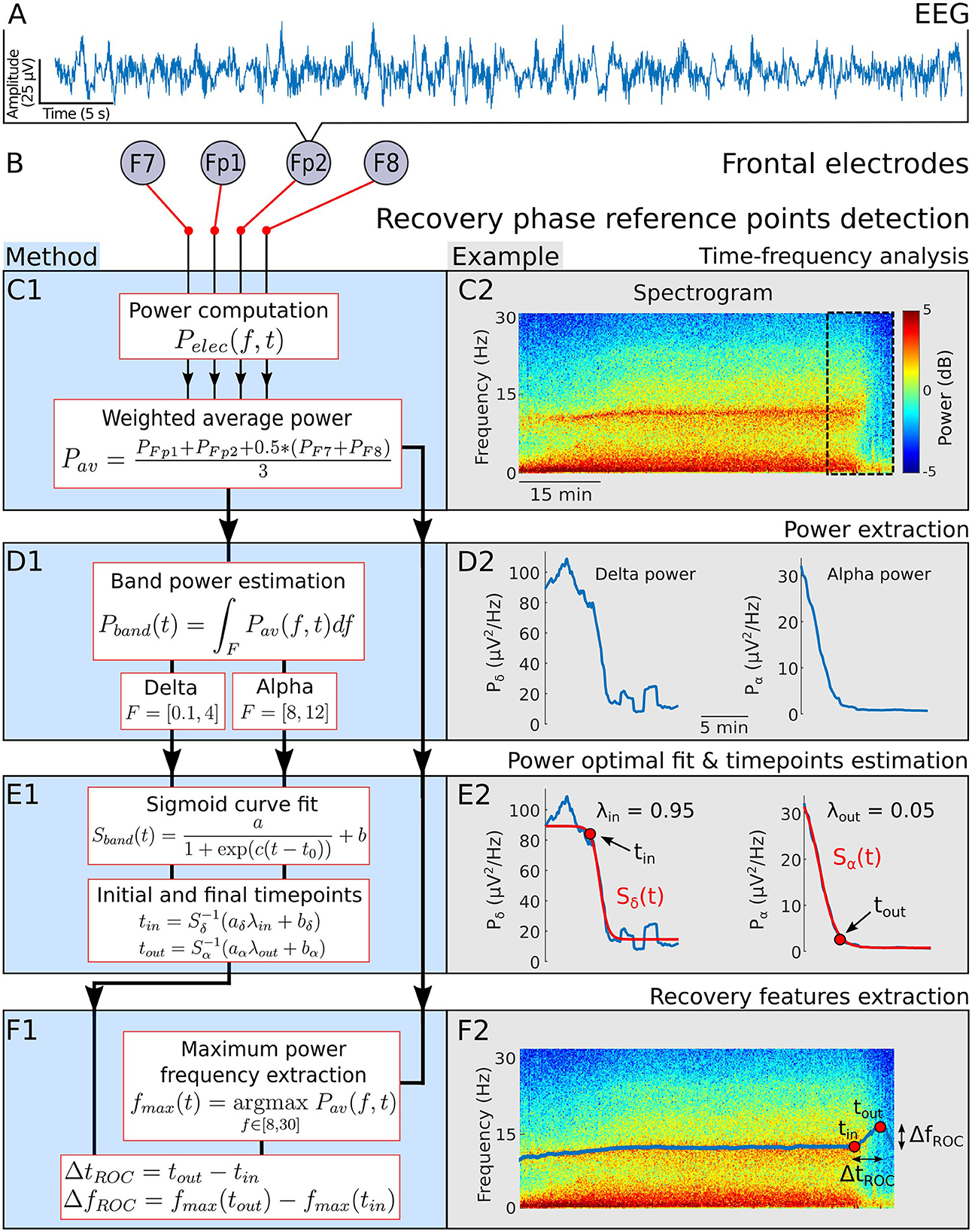
Figure 1. Emergence phase detection. (A) EEG signal. (B) Frontal electrodes. (C) 1- Power of a weighted average of the four EEG channels. 2- Spectrogram visualization for a single patient during general anesthesia. (D) 1-α−band power Pα and δ−band power Pδ 2- Power Pα and Pδ computed from the spectrogram 20 min before the end of anesthesia. (E) 1- Sigmoid function Sband used to fit Pα and Pδ during the recovery phase. Definition of the final time tin (resp. tout) for which the fit Sδ (resp. Sα) reaches for the first time the threshold aλin+b (resp. aλout+b). 2- Fit examples and detection of tin and tout. (F) 1- Maximum power frequency fmax and definition of the duration and frequency shifts during recovery. 2- Extracted fmax and positioned tin and tout on the associated spectrogram.
To account for the predominant role of the frontal cortex in the genesis of the α−band during GA (25, 26), we averaged the spectrograms with different weights: we halved the contribution of electrodes F7 and F8 (Figures 1, 2). We then followed the α−band power Pα and δ−band power Pδ. The signal power within a band Pband(t) is equal to the area under the curve Pav(f, t), where the frequency f varies in a given band, as shown in Figures 1, 2. Specifically,
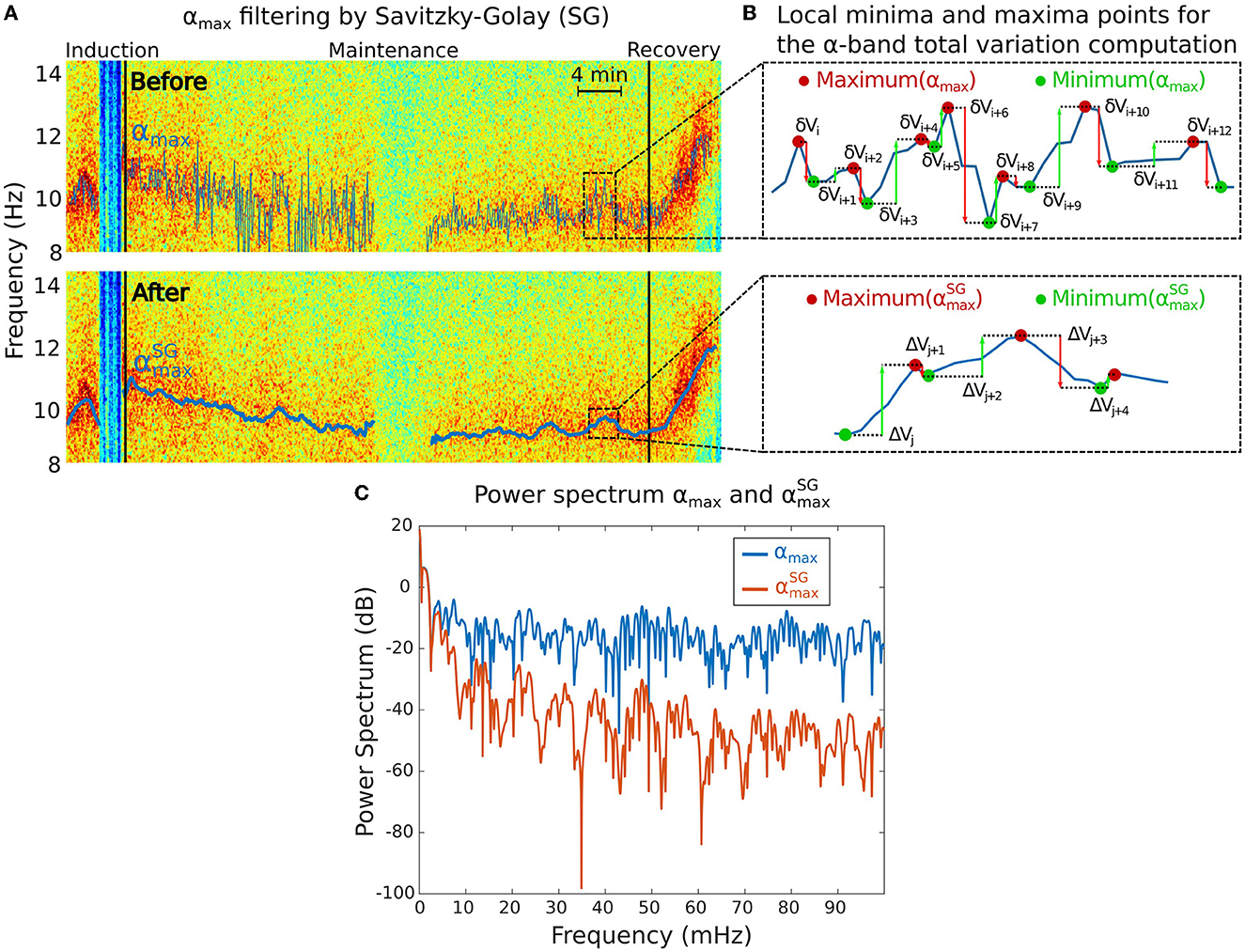
Figure 2. Total variation Vα analysis associated to the α−band. (A) Maximum power frequency αmax of the α−oscillations before (top) and after (bottom) applying the Savitzky-Golay (SG) filter to remove the high frequencies. (B) Reduction of the local minima and maxima variations of the αmax from the initial signal (top) to the filtered one (bottom). (C) Power spectra of αmax before (blue) and after (red) SG filtering showing that only the slowest oscillations remain in the filtered signal.
We fitted separately the powers Pδ, Pα with a sigmoid function
where k = δ or α) (Figures 1, 2). The parameters a, b, c and t0 are estimated by minimizing error integral
Where Tf is the last time where the EEG recordings terminates. The time point tin is defined as the first time where the sigmoid curve Sδ crosses the threshold with λin = 0.05. Equivalently, , thus
We also determined the frequency curve fmax with maximal power in the range (8-30) Hz (Figures 1, 2) using
Similarly, we define the time point tout as the first time where Sδ crosses with λout = 0.95, thus
Using these two reference points tin and tout, we deduced the duration and the frequency shifts associated with the α−band emergence trajectory (Figures 1, 2)
2.3. Segmenting IES and α suppressions
The IES segmentation procedure follows the steps presented in Sun and Holcman (14) that we briefly recall. We first filter the EEG signal S(t) in the range [8,16] Hz to get Sα(t). We normalize Sα(t) by its Root-Mean-Square to obtain Ŝα(t). We then estimated the upper and lower envelops of S(t) and Ŝα(t) by interpolating their local maxima and minima. We applied the difference D(t) and Dα(t) between the respective upper and lower envelops, and defines two threshold values for the IES:
We then define the IES (resp. αS) time segment as the ensemble satisfying the conditions
Finally, we aggregate the time intervals of ΩIES and ΩαS into segments such that each pair of consecutive points of the segment matches with the known sampling frequency. To smooth the effect of the hard thresholding, we used morphological erosion and dilation operations (27) to obtain the IES and αS duration intervals.
2.4. Mathematical indicators associated to iso-electric suppressions, α and δ bands
• The total time spent in IES is the sum of time segments during induction in ΩIES. For each ith segment Ti which starts (resp. ends) at time Ti, start (resp. Ti, end), we defined
• The longest IES event is equal to the maximum of the duration present in ΩIES during induction.
• The α−band relative power Pα(t) at time t describes the proportion of energy in the range [8, 12] Hz with respect to [0.1, 45] Hz, as defined by
To compute the mean value of the relative α−band power during maintenance, we use the discretized sum approximation
• The mean value of the δ−band relative power is obtained following the procedure of Pδ.
• The maximum power frequency αmax within the α− band is the frequency for which the power is maximal and defined outside of IES or αS regions.
where
The maximum frequency αmax(t) contains multi-scale oscillations that do not necessarily reflect physiological information. We thus decided to smooth αmax(t) using the adaptive Savitzky-Golay smoothing filter (28) to keep lower frequencies (Figure 2A). We used a sliding window of 2 min and 5 s step size with order 1 polynomial regression. We denote the resulting filtered signal.
• The fluctuations of the α−band dominant frequency are measured using the total variation Vα of the function (Figure 2B). This quantity sums the cumulated amplitude of local oscillations in each time intervals and thus measures the deviation of the maximum α−band frequency dynamics with a flat line.
The total variation is computed over a total of M periods of time, where the α−band is present. We apply the sum of the absolute difference between two consecutive frequency time points over the M time segments. For the kth time segment, we use the local maxima and minima time discretization , (see Figure 2B) so that
• The δ−band total variation Vδ is computed with the same computational steps as the α−band with the maximum power frequency δmax defined by
where
We compare the spectral properties of the signal before and after filtering (Figure 2C).
2.5. Pearson linear correlation coefficient and Bayes factors
The Pearson correlation coefficient rxy is used to evaluate the correlation between two variables, x = (x1,.., xn) and y = (y1,.., yn), in a sample of n points, defined by
where the sample mean is with similar definition for .
The null hypothesis H0 is defined as no correlation between x and y, while H1 hypothesis postulate that a correlation exists (29). To provide evidences in favor of the null hypothesis, we use the Bayes factor BF01 by evaluating the ratio of the conditional probability of the observable y given the hypothesis H0 given by
We shall now rewrite each hypothesis in terms of linear regression by considering
where (α, β) are the regression estimates and ϵ~N(0, σ2I), where the constant σ is fixed. The marginal probabilities can be written
Where γ = 0 or 1 and θγ are the model parameters (a, b, σ2). For we add a scalar g in the model parameters. When γ = 1, we have
and
Thus the probability is given by
We follow the steps described in Liang et al. (30) based on Zellner g-priors to get an expression for these probabilities
After integrating out all the parameters, we obtain the analytical expression for the Bayes factor
which depends on p is the number of covariates in H1 (30–32).
2.6. Partial correlation
The partial correlation coefficient rxy∣z measures the correlation between the data x and y while controlling for z. It is defined by
The corresponding Bayes factor compares the models
The associated Bayes factor is given by Liang et al. (30), Wetzels and Wagenmakers (31) and Rouder et al. (32)
where (R0, R1) are the coefficients of determination in (H0, H1), (p, p′) are the number of covariates in (H0, H1).
3. Results
To search for possible causal correlation in the EEG between the induction, maintenance phases and the recovery phase of anesthesia, we shall apply the indices presented in the Section 2. We start by estimating the time and frequency shifts of the α−band trajectory during recovery and use them to explore the possible correlations with the total time spent in suppression (iso-electric EEG), a marker of brain sensitivity (5). We will also consider the possible correlation of the frequency shift with respect to the longest suppression induced by a propofol bolus during induction. Finally, we will assess the possible correlation using the total variation, which measures the variation of the band frequency maximum amplitude over time.
3.1. Duration and frequency shifts during the α−band emergence trajectory
The EEG signal in the maintenance phase are dominated by two frequency bands: δ−band (0.1–4 Hz) and α−band (8–12 Hz) as depicted in Figures 1A–C. Once the hypnotic injection is stopped, the first step of the recovery phase is characterized by a successive decay of the delta and alpha activity decay. To quantify the time and spectral changes occurring in the EEG during the recovery phase, we shall detect two reference time points tin and tout, associated with the maximum power frequency within the α−band. The first time tin is the first instant where the δ−band disappears from the continuous steady-state regime of the maintenance phase. Thereafter, the time tout corresponds to the instant where the α−band power reaches a lower plateau threshold value.
We identify tin by applying an optimal fitting procedure of the power Pδ (Equation 2) with a sigmoid curve Sδ (Equation 4) and we deduce the first time where Sδ has reached the threshold λin = 95% of the transient trajectory (see Section 2 and Figure 1D).
Similarly, we fitted the power Pα (Equation 3) with a sigmoid curve Sα (Equation 4) and defined the time tout as the first instant where Sα has reached λout = 5% of the transient trajectory left to cross (Figure 1E).
Finally, we use this time identification to deduce the duration shift of the α−band emergence trajectory for two population cohorts: for the children cohort, we found the duration is given by ΔtROC = 7.8[4.2, 10.2] (Median [IQR]) min and the associated frequency shift is given by ΔfROC = 3.3[1.8, 5.0] Hz. For the adult cohort, we found ΔtROC = 7.3[5.8, 10.4] min and ΔfROC = 1.9[1.3, 2.5] Hz. Interestingly, the distribution of duration ΔtROC is similar for both adults and children (Table 1).
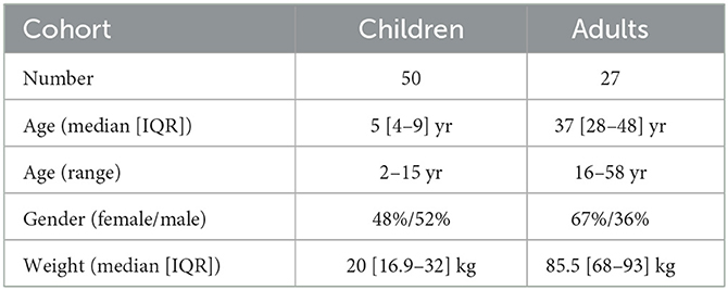
Table 1. Patients demographic information.
3.2. Stability of the α−band measured by the total variation
To quantify the stability of the α−band, we estimated how it varies vary from a straight line by using the total variation, a quantity that accounts for any form of oscillation. However, a correlation analysis revealed that the total variation of the α−band is independent of the presence of any suppression patterns such as IES or αS. Indeed, the time spent in suppressions is uncorrelated to the α−band total variation (Figures 3A, B). This result suggests that the IES and total variation can be treated as independent variables in the EEG analysis. The correlation coefficients for the α−suppression (resp. IES) were r = 0.04, p = 0.83 and the Bayesian factor BF01 = 6.6 (resp. r = −0.06, p = 0.75, BF01 = 6.4). We thus reject with moderate evidence the hypothesis that high oscillations of the α−band would be correlated to αS.
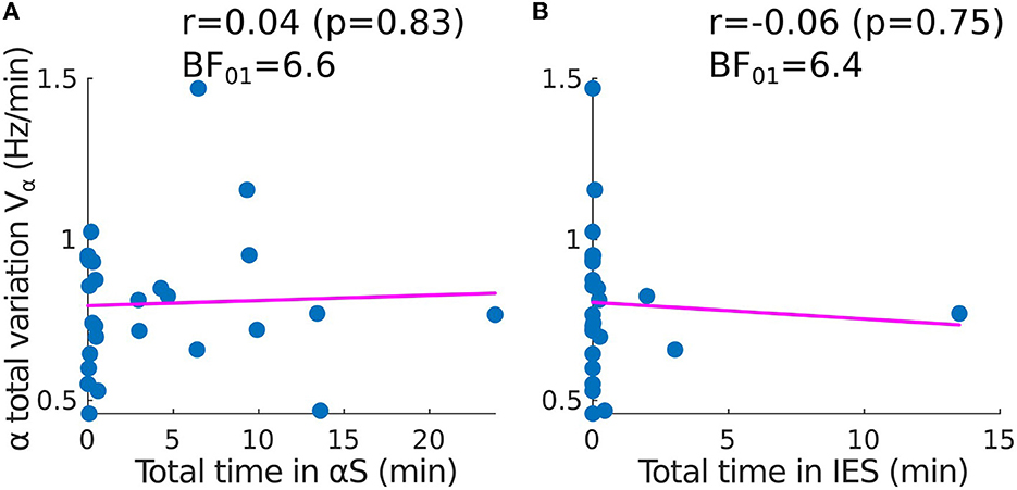
Figure 3. Correlation between the time spent in suppressions and the total variation of the α−band (adult population). Scatter plots and correlations (Pearson r, p-value p) between the α−band total variation Vα and (A) the total time spent in α−suppressions (frequency loss in the α−band), (B) the total time spent in IES SIES.
3.3. α−band and IES during induction and maintenance are not correlated with α−band emergence trajectory
3.3.1. Statistical correlations for the children cohort
To determine whether the statistical properties of the recovery phase can be anticipated, we first examined possible correlations from the different variables that we extracted and in particular from the IES for children. We studied the total time spent in IES during maintenance and the IES duration induced by a strong propofol bolus at the end of induction (Figures 4A–D).
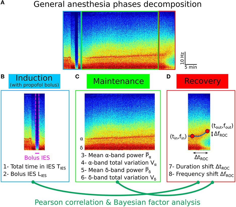
Figure 4. Pearson correlation analysis of the three phases of general anesthesia. (A) Spectrogram (time-frequency) representation of the EEG signal during the three phases: induction (blue), maintenance (green), recovery (red). (B) Statistical parameters collected during induction: 1- Total time in IES SIES, 2- Longest IES duration LIES. (C) Statistical parameters collected during maintenance: 3- Mean α−band power , 4- α−band total variation Vα, 5- Mean δ−band power , 6- δ−band total variation Vδ. (D) Statistical parameters collected during recovery: 7- Duration shift ΔtROC, 8- Frequency shift ΔfROC.
We found that (see Section 2.4) the total time spent in IES SIES = 1.2[0.4, 1.9] min and the longest time spent in IES (induced by propofol bolus) LIES = 0.3[0.1, 0.7] min.
Secondly, we quantified the Pearson correlation (Figure 5A) along with its p-value and found that the total duration of the IES (resp. longest IES) is not correlated neither to the duration of recovery ΔtROC [r = −0.27, p = 0.06 (resp. r = −0.08, p = 0.57)] nor to the frequency shift ΔfROC [r = −0.13, p = 0.37 (resp. r = −0.06, p = 0.70)], as shown in Figure 5. At this stage, we conclude that no significant correlations are revealed by the transient parameters associated with the electrical absence of the EEG signal.
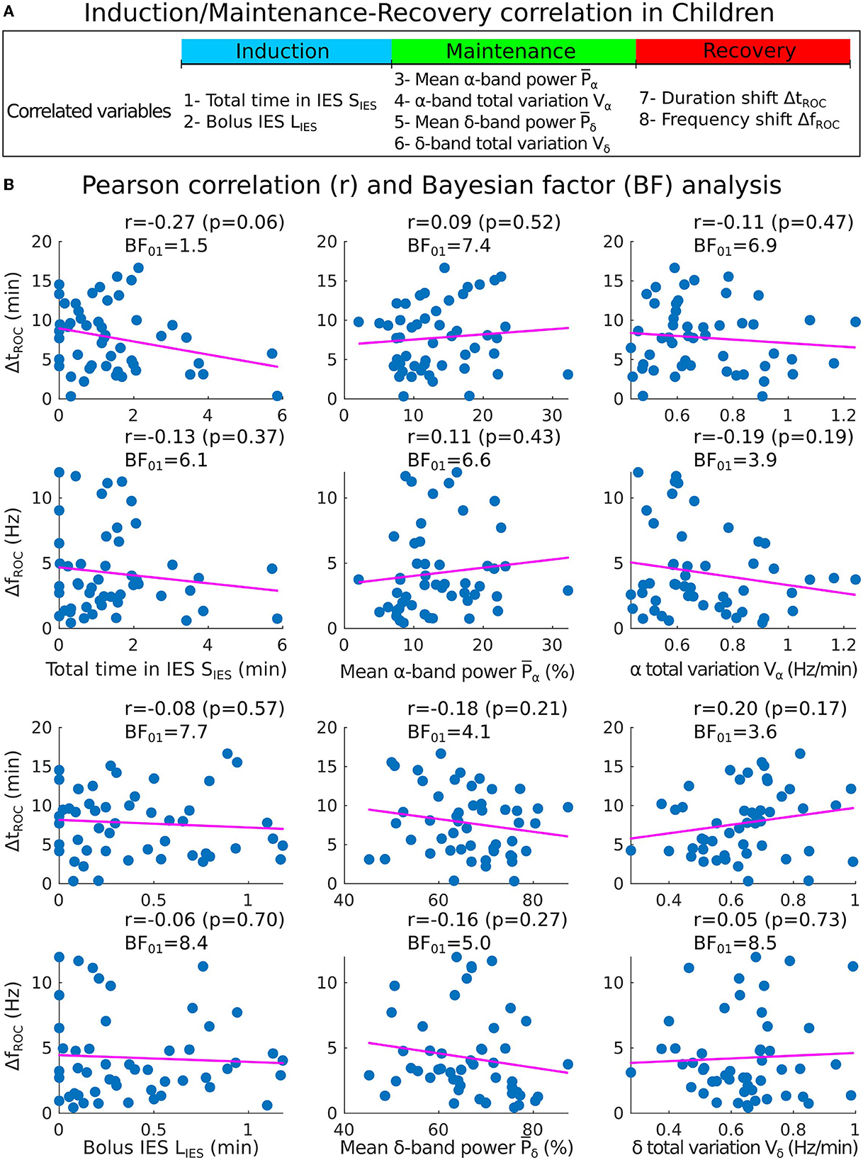
Figure 5. Correlations analysis of induction and maintenance with recovery for 50 children. (A) Summary of the statistical parameters collected from the induction and maintenance phases (total time in IES SIES, bolus IES duration LIES, mean α−band power and α−band total variation Vα) and the recovery phase markers (duration shift ΔtROC and frequency shift ΔfROC). (B) Scatter plots and Pearson (coefficient r, p-value p, Bayes factor BF01) correlations between ΔtROC (ΔfROC) and SIES, LIES (first column), , (second column), Vα, Vδ (third column).
To further study the possible correlations, we computed the mean power of the α−band during the maintenance and the total variation Vα which measures the deviation of the maximum frequency fα of the α−oscillations from a flat curve (Figures 4C, D). We reported that the mean power and Vα = 0.64[0.56, 0.80] Hz/min. We estimated the correlations between (resp. Vα) and either ΔtROC [r = 0.09, p = 0.53 (resp. r = −0.09, p = 0.53)] or ΔfROC [r = 0.11, p = 0.43 (resp. r = −0.16, p = 0.27)], but found insignificant outcome.
We repeated the procedure with the same parameters derived from the δ−band and obtained and Vδ = 0.65[0.54, 0.72] Hz/min. Similarly, the correlations between (resp. Vδ) and either ΔtROC (r = −0.18, p = 0.21 (resp. r = 0.20, p = 0.17)) or ΔfROC (r = −0.16, p = 0.2 (resp. r = 0.05, p = 0.73) remained non-significant.
However, in our current state, we only failed to reject the null hypothesis of no correlation when obtaining a p-value greater than the 5% acceptance level. To support the null hypothesis H0, we computed the associated Bayes factor (30, 31, 33) BF01 which is the ratio of the probability between the null hypothesis and the alternative one H1 considering our data points. According to Jeffreys evidence category scheme (29) for the Bayes factor, our data mostly shows moderate evidence for H0 as shown in Table 2. We found an anecdotal evidence for H0 between the total time spent in IES SIES and the duration shift ΔtROC. To conclude, the statistics associated with the presence or absence of the α−band do not show any significant correlation with the frequency and duration shifts of the α−band emergence dynamics. In particular, an unstable α−band does not necessarily lead to a longer time of return to consciousness.
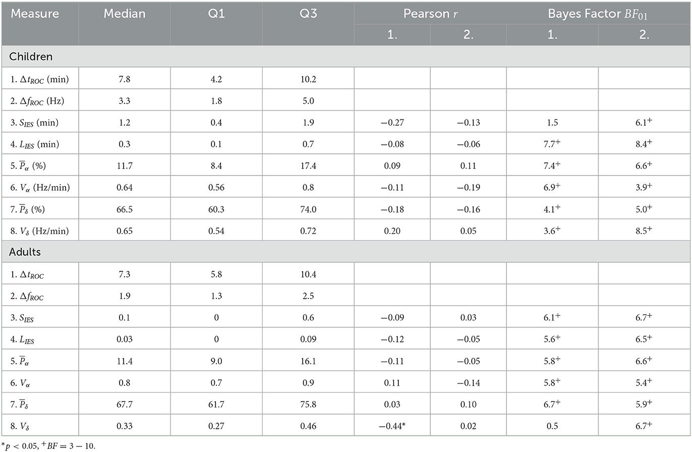
Table 2. Medians, inter-quartile ranges, Pearson correlations, and Bayes factor of EEG statistical features.
3.3.2. Statistical correlations in the adults cohort
We applied the same procedure for adults sedated with propofol target controlled infusion (TCI) protocol. Having, SIES = 0.1[0, 0.6] min and LIES = 0.03[0, 0.09] min, we report with moderate evidence that the total time in IES (resp. longest IES) was not correlated neither to the duration shift ΔtROC [r = −0.09, p = 0.65, BF01 = 6.1 (resp. r = −0.12, p = 0.54, BF01 = 5.6)] nor the frequency shift ΔfROC [r = 0.02, p = 0.88, BF01 = 6.7 (resp. r = −0.05, p = 0.81, BF01 = 6.5)] (Figures 6A, B).
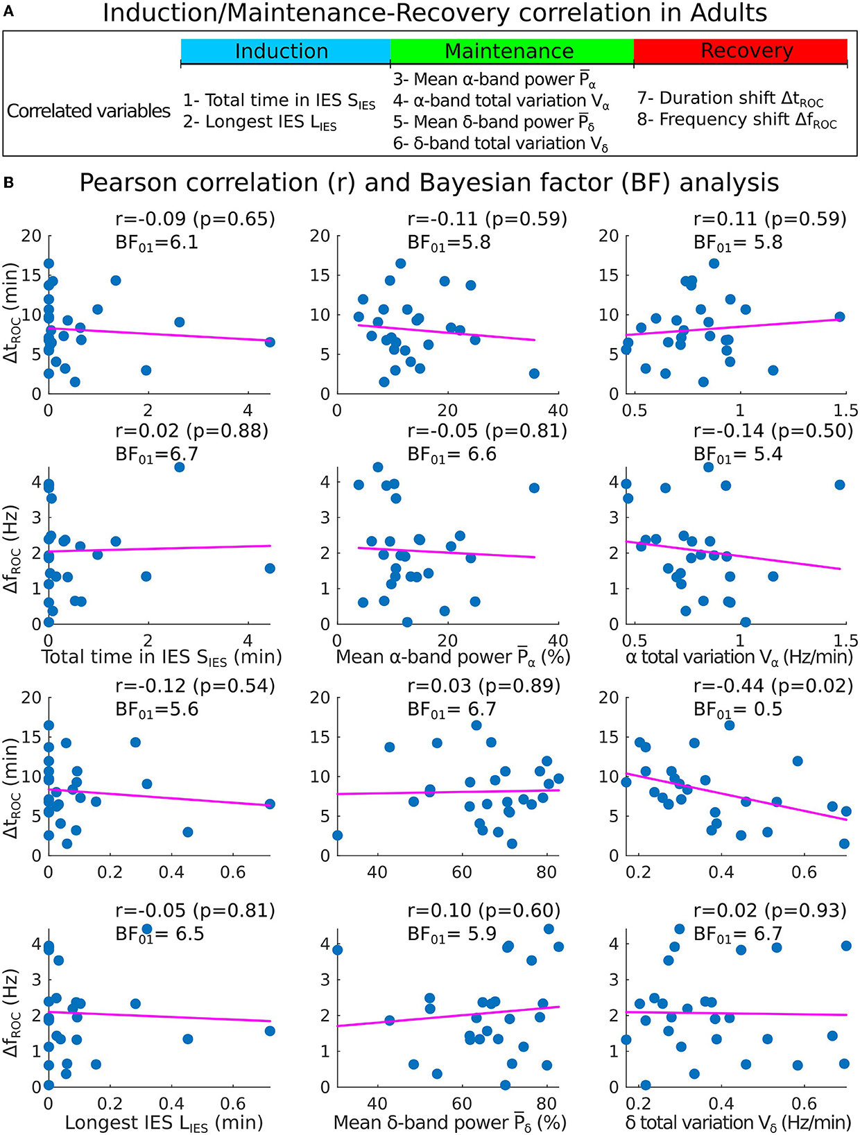
Figure 6. Correlations analysis of induction and maintenance with recovery for 27 adults. (A) Summary of the statistical parameters collected during induction and maintenance phases (SIES, LIES, and Vα) and the recovery phase (ΔtROC and ΔfROC). (B) Scatter plots and Pearson (coefficient r, p-value p, Bayes factor BF01) correlations between ΔtROC (ΔfROC) and SIES, LIES (first column), , (second column), Vα and Vδ (third column).
We also report the values for the mean power , Vα = 0.8[0.7, 0.9] Hz/min, and Vδ = 0.33[0.27, 0.46] Hz/min. We found again moderate evidence of null correlations between the power (resp. Vα) and neither ΔtROC [r = −0.11, p = 0.59, BF01 = 5.8 (resp. r = 0.11, p = 0.59, BF01 = 5.8)] nor ΔfROC [r = −0.05, p = 0.81, BF01 = 6.6 (resp. r = −0.14, p = 0.50, BF01 = 5.4)].
However, for the δ−band parameters, the correlation between Vδ and ΔtROC was significant (r = −0.44, p = 0.02, BF01 = 0.5) but the evidence for the alternative hypothesis H1 was anecdotal. For the remaining parameters, moderate evidence of no significant statistical correlations were found.
We conclude using a statistical approach estimated over two cohorts of adults and children that the duration of the emergence trajectory, characterized by a shift of the maximum α−band is not significantly correlated neither with the fraction of iso-electric suppression nor with the α−band or δ−band dynamics measured by its power and total variation. Thus, these EEG parameters obtained during induction and maintenance of GA cannot be directly used to explain the duration of the α−band emergence trajectory.
3.3.3. Demographic factors provide insignificant role in the correlations analysis
To account for the impact of demographic factors, the correlations of our features were computed while controlling for age, gender, and weight as covariates. By doing so, we eliminated the effect of confounding covariates that could be numerically related to our features of interest. The partial correlation coefficients and their Bayes factors (see Section 2) are shown in Table 3. A significant partial correlation (r = −0.29, p < 0.05) was found between the total time spent in IES and the duration shift for the children cohort, though the Bayes factor BF01 = 475 suggests decisive evidence for H0. In the adult cohort, a moderate but non-significant correlation (r = −0.37, p = 0.07) between the δ total variation and the duration shift was found, with decisive evidence for H0 (BF01 = 257). For the remaining parameters, the Bayes factors support at least very strongly the null hypothesis H0.
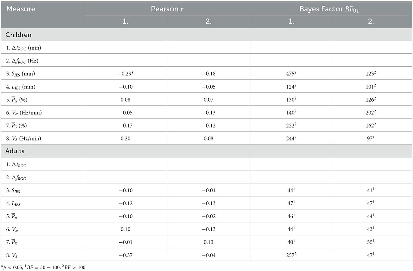
Table 3. Partial correlations and Bayes factor of EEG statistical features.
3.4. Clinical recovery duration are uncorrelated with the IES and bands parameters
To compare with the results described in the above subsections, we defined the clinical recovery duration from the instant where the hypnotic injection is turned off to the extubation time, where the patient showed the first signs of awareness or recovery of effective spontaneous ventilation. We report with moderate evidence, no correlations between IES total (resp. longest bolus) duration and the extubation time [r = −0.02, p = 0.88, BF01 = 8.8 (resp. r = −0.09, p = 0.53, BF01 = 7.3)] (Figures 7A, B). Additionally, a moderate evidence of insignificant correlation for the α−band total variation was found (r = −0.01, p = 0.97, BF01 = 8.9). For the remaining band parameters, only anecdotal evidences for the null hypothesis were found despite the moderate correlation obtained (: r = −0.24, p = 0.10, BF01 = 2.2; : r = 0.25, p = 0.09, BF01 = 2.2; Vδ: r = −0.29, p = 0.04, BF01 = 1.1).
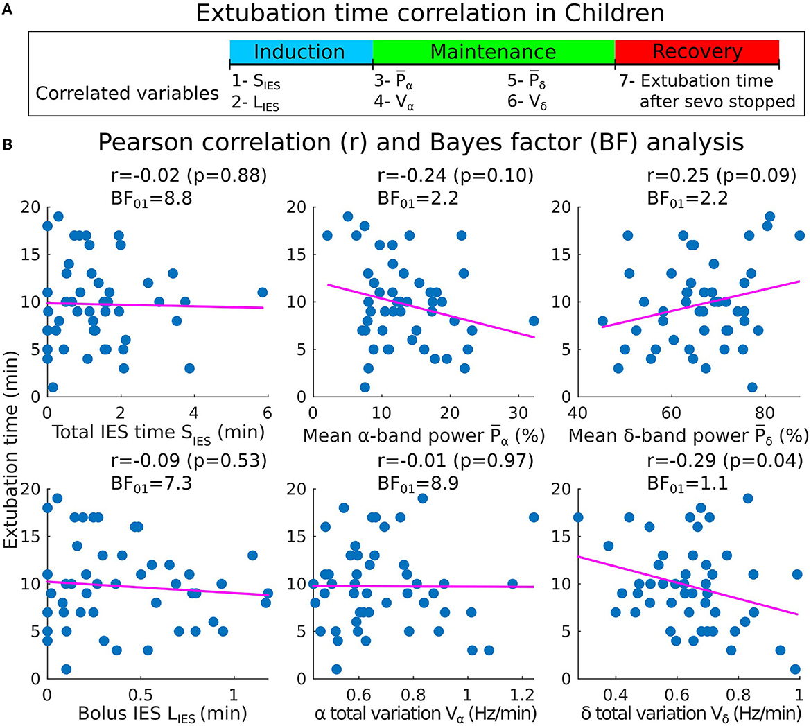
Figure 7. Pearson correlations between the induction/maintenance phases and the extubation time after the sevoflurane has stopped (children cohort). (A) Extubation time after the administration of sevoflurane has stopped vs. SIES, LIES, and Vα collected during induction and maintenance. (B) Scatter plots and Pearson correlations (coefficient r, p-value p) between the extubation time and SIES, LIES (first column), , Vα (second column), and Vδ (third column).
3.5. Bayesian inferences shows that longer emergence duration is unlikely to follow long IES duration
To investigate whether a long cumulated IES duration could predict a long α−band emergence duration, we computed the associated empirical conditional probability Pr{tROC>TROC∣SIES>TIES}. Using the distribution shown in Table 2, we set a threshold at the 70th percentile, resulting in TROC = 10s and TIES = 1.8 s for the children cohort. We found that P(tROC>TROC∣SIES>TIES) = 0.21, while for the adult population, the appropriate threshold changed to TIES = 0.5 s and the conditional probability was 0.25.
In the children population, we further computed the conditional probability of a long cumulative IES duration when a long IES duration was caused by a propofol bolus. Setting a threshold TBOL = 0.5 for deciding of the population associated with a long bolus suppression, we found the P{SIES>TIES∣LIES>TBOL} = 0.64. To conclude, a Bayesian conditional approach reveals that longer emergence duration is unlikely to follow long IES duration. However, there is a relatively high probability that a longer cumulative IES duration will follow a long IES bolus duration.
4. Discussion
In the present study, we used several mathematical indices to quantify the δ and α−bands and to explore the possible correlations of these parameters computed during induction and maintenance with the recovery phase. During induction, we considered the longest IES (induced by a bolus of propofol in children). While adults underwent intravenous hypnotic injection, induction with children starts with inhalation of sevoflurane followed by a bolus of propofol to avoid oro-tracheal intubation complications (34, 35). During maintenance, we computed the mean power of the α−band and the total variation Vα (Equation 21), a measure of the α−oscillations maximum amplitude instability. Small values of Vα are associated with low fluctuations around a flat line. Conversely, the higher Vα, the larger is the deviation. Thus, a high value of Vα characterizes a global instability during anesthesia. During both the induction and maintenance phases, we estimated the total time spent in IES. Finally, during the recovery phase, we estimated the frequency and duration shifts associated to the α−band emergence trajectory from the EEG time-frequency representation, as reported in previous research (25).
The present analysis revealed in general no relationship between the parameters we introduced (Figures 5, 6) in the different phases. These results invalidate our hypothesis concerning a possible correlation between the longest or total IES duration and a longer duration of the α−band emergence trajectory.
Furthermore, our results indicate that the IES durations are not only unrelated with the α−band emergence trajectory, but also with the clinical recovery duration, starting from the instant the hypnotic injection is turned off to the extubation time (Figure 7), where the patient showed first signs of awareness or recovery of spontaneous ventilation and which does not directly follow the end of the emergence trajectory. These findings are consistent with the results reported in Shortal et al. (36), where IES duration was also found to be uncorrelated with the degree of cognitive impairment after anesthesia, as measured by fitting the decay of expired isoflurane to a single exponential.
In addition to the lack of correlation between IES duration and the α−band emergence trajectory in the EEG time-frequency representation, our results also indicate that the α−band dynamics do not show further correlations as revealed by the total variation (Equation 21) of the α−band maximum frequency αmax. Previous research has suggested that a high total variation could reflect a constant re-adjustment that could be induced by real-time hypnotic concentration variation (37, 38). However, our results, which show insignificant correlation between the time spent in suppressions and the α−band total variation (Figure 3), reject this hypothesis. The total variation Vα could either increase due to a change in the hypnotic concentration or due to the intrinsic response of the brain to a fixed concentration. In the latter case, these changes could represent an instability of thalamo-cortical neuronal networks to converge to a stable constant α−oscillations, which are considered as a marker of brain synchronization (20).
Moreover, the mean α−band power has been used to monitor the depth of anesthesia and as a possible predictor for the arrival of IES (5, 13). Lower values of the power reflects a vulnerable brain and could have been associated to a longer time of emergence. However, this hypothesis was not confirmed in our analysis (Figure 7) where we found insignificant correlation between the mean power and the extubation time.
Based on these findings, it is plausible to suggest that the recovery of the brain from constant anesthetic injection is a memoryless process. Considering that propofol and sevoflurane, both of which are GABAergic agonists (39), enhance the role of inhibitory neurons, the level of neuronal activity mainly depends on the speed at which the hypnotic is absorbed (induction) or eliminated (recovery) by the brain. Indeed, general anesthesia causes thalamic neurons to intrinsically change states (40). During induction, these neurons typically switch from spiking to bursting, while during recovery the switch is from bursting to fast spiking. This is consistent with the changes seen in EEG, where a decrease in the δ (0.1–4 Hz) power and an increase of β (12–30 Hz) power indicate a return to normal neuronal activity (25). During the maintenance phase, the brain has theoretically acclimated to the hypnotics by displaying steady-state neural dynamics.
Statistical analysis
In this study, statistical analysis was conducted using MATLAB R2021a software. A significance level of α = 0.05 was used throughout the analysis. Qualitative variables were expressed as percentages and quantitative variables were expressed as the median (Inter-Quartile Range: [IQR]). Correlations between variables were determined using the Pearson (r) correlation test. To provide evidence in favor of the null hypothesis, Bayes factor (BF01) was used. No statistical outliers were found or removed in the correlation analyses.
General statement about general anesthesia
This study is a prospective observational study that included patients who underwent elective procedures requiring standardized general anesthesia procedure. The EEG data used in the study were collected from Louis-Mourier Hospital in Colombes, France between October 2019 and September 2021, in compliance with the evaluation of clinical practice and included a total of 77 patients (50 children and 27 adults), along with their demographic factors and other clinical information. Patients with incomplete or corrupted data were not included in the study. For adult patients, general anesthesia was induced through the intravenous administration of either sufentanil in iterative bolus doses between 5 and 15 gamma or TCI remifentanil ranging from 2.5 to 6 ng.ml−1 for the opioid agent, and propofol for the hypnotic agent with a TCI ranging from 3 to 10 μg.ml−1 (19). Patients were then intubated following curarization with rocuronium (0.5–0.7 mg.kg−1).
For children, the hypnotic agent sevoflurane was administered through inhalation with an initial concentration of 6%. Following insertion of the intravenous line, the children received 0.1 μg.kg−1 of sufentanil or 15 μg.kg−1 of alfentanil. Propofol was then administered in one or more bolus doses until the appearance of iso-electric suppressions for oro-tracheal intubation. The initial quantity of propofol was calibrated according to the child's weight using a 2 mg.kg−1 rule. The anesthesiologist made adjustments to the concentrations depending on the patient's reaction and the anesthesia phase. Additional drugs were given at the discretion of the anesthesiologist as long as the standard of care was respected. Finally, to prepare for the recovery and extubation phase, the concentration of sevoflurane was typically lowered to values between 0.5 and 2.5% 5 to 10 min before complete shut off.
Data availability statement
The raw data supporting the conclusions of this article will be made available by the authors, without undue reservation.
Ethics statement
Ethical review and approval was not required for the study on human participants in accordance with the local legislation and institutional requirements. Written informed consent to participate in this study was provided by the participants and/or the participants' legal guardian/next of kin.
Author contributions
DL and DH: designed research. CS and DH: analyzed data and wrote the manuscript. DL: collected data and corrected the manuscript. All authors contributed to the article and approved the submitted version.
Funding
DH research was supported by a grant ANR NEUC-0001, PSL and CNRS pre-maturation and the European Research Council (ERC) under the European Union's Horizon 2020 research and innovation programme (grant agreement no. 882673).
Conflict of interest
The authors declare that the research was conducted in the absence of any commercial or financial relationships that could be construed as a potential conflict of interest.
Publisher's note
All claims expressed in this article are solely those of the authors and do not necessarily represent those of their affiliated organizations, or those of the publisher, the editors and the reviewers. Any product that may be evaluated in this article, or claim that may be made by its manufacturer, is not guaranteed or endorsed by the publisher.
Abbreviations
EEG, electroencephalogram; GA, General anesthesia; IES, Iso-electric suppression; ROC, Recovery Of consciousness.
References
1. Worrell GA, Jerbi K, Kobayashi K, Lina JM, Zelmann R, Le Van Quyen M. Recording and analysis techniques for high-frequency oscillations. Progr Neurobiol. (2012) 98:265–78. doi: 10.1016/j.pneurobio.2012.02.006
2. Jaffard S, Meyer Y, Ryan RD. Wavelets: Tools for Science and Technology. SIAM. (2001). doi: 10.1137/1.9780898718119
3. Schomer DL, Da Silva FL. Niedermeyer's Electroencephalography: Basic Principles, Clinical Applications, and Related Fields. Lippincott Williams & Wilkins (2012). doi: 10.1093/med/9780190228484.001.0001
4. Ciuciu P, Abry P, Rabrait C, Wendt H. Log wavelet leaders cumulant based multifractal analysis of EVI fMRI time series: evidence of scaling in ongoing and evoked brain activity. IEEE J Select Top Signal Process. (2008) 2:929–43. doi: 10.1109/JSTSP.2008.2006663
5. Cartailler J, Parutto P, Touchard C, Vallée F, Holcman D. Alpha rhythm collapse predicts iso-electric suppressions during anesthesia. Commun Biol. (2019) 2:1–10. doi: 10.1038/s42003-019-0575-3
7. Averbuch AZ, Neittaanmäki P, Zheludev VA. Acoustic detection of moving vehicles. In: Spline and Spline Wavelet Methods With Applications to Signal and Image Processing. Springer (2019). p. 219–39. doi: 10.1007/978-3-319-92123-5_12
8. Flandrin P, Amin M, McLaughlin S, Torrésani B. Time-frequency analysis and applications. IEEE Signal Process Mag. (2013) 30:19. doi: 10.1109/MSP.2013.2270229
9. Spinnato J, Roubaud M, Burle B, Torrésani B. Detecting single-trial EEG evoked potential using a wavelet domain linear mixed model: application to error potentials classification. J Neural Eng. (2015) 12:036013. doi: 10.1088/1741-2560/12/3/036013
10. Dora M, Holcman D. Adaptive single-channel EEG artifact removal with applications to clinical monitoring. IEEE Trans Neural Syst Rehabil Eng. (2022) 30:286–95. doi: 10.1109/TNSRE.2022.3147072
11. Dora M, Jaffard S, Holcman D. The WQN algorithm to adaptively correct artifacts in the EEG signal. Appl Comput Harmonic Anal. (2022) 61:347–56. doi: 10.1016/j.acha.2022.07.007
12. Hastie T, Tibshirani R., Friedman J. H. The Elements of statistical Learning: Data Mining, Inference, and Prediction, Vol. 2. Springer (2009).
13. Shao YR, Kahali P, Houle TT, Deng H, Colvin C, Dickerson BC, et al. Low frontal alpha power is associated with the propensity for burst suppression: an electroencephalogram phenotype for a “vulnerable brain”. Anesth Anal. (2020) 131:1529. doi: 10.1213/ANE.0000000000004781
14. Sun C, Holcman D. Combining transient statistical markers from the EEG signal to predict brain sensitivity to general anesthesia. Biomed Signal Process Control. (2022) 77:103713. doi: 10.1016/j.bspc.2022.103713
15. Plummer GS, Ibala R, Hahm E, An J, Gitlin J, Deng H, et al. Electroencephalogram dynamics during general anesthesia predict the later incidence and duration of burst-suppression during cardiopulmonary bypass. Clin Neurophysiol. (2019) 130:55–60. doi: 10.1016/j.clinph.2018.11.003
16. Kay DC, Pickworth WB, Neidert GL, Falcone D, Fishman PM, Othmer E. Opioid effects on computer-derived sleep and EEG parameters in nondependent human addicts. Sleep. (1979) 2:175–91. doi: 10.1093/sleep/2.2.175
17. Smith NT, Dec-Silver H, Sanford TJ Jr, Westover CJ Jr, Quinn ML, Klein F, et al. EEGs during high-dose fentanyl-, sufentanil-, or morphine-oxygen anesthesia. Anesth Anal. (1984) 63:386–93. doi: 10.1213/00000539-198404000-00002
18. Egan TD. Remifentanil pharmacokinetics and pharmacodynamics: a preliminary appraisal. Clin Pharmacokinetics. (1995) 29:80–94. doi: 10.2165/00003088-199529020-00003
19. Absalom AR, Mason KP. Total Intravenous Anesthesia and Target Controlled Infusions. Springer (2017).
20. Brown EN, Lydic R, Schiff ND. General anesthesia, sleep, and coma. N Engl J Med. (2010) 363:2638–50. doi: 10.1056/NEJMra0808281
21. Purdon PL, Sampson A, Pavone KJ, Brown EN. Clinical electroencephalography for anesthesiologistspart I: background and basic signatures. Anesthesiology. (2015) 123:937–60. doi: 10.1097/ALN.0000000000000841
22. Hughes SW, Crunelli V. Thalamic mechanisms of EEG alpha rhythms and their pathological implications. Neuroscientist. (2005) 11:357–72. doi: 10.1177/1073858405277450
23. Cascella M, Bimonte S, Muzio MR. Towards a better understanding of anesthesia emergence mechanisms: research and clinical implications. World J Methodol. (2018) 8:9. doi: 10.5662/wjm.v8.i2.9
24. Kim H, Moon JY, Mashour GA, Lee U. Mechanisms of hysteresis in human brain networks during transitions of consciousness and unconsciousness: theoretical principles and empirical evidence. PLoS Comput Biol. (2018) 14:e1006424. doi: 10.1371/journal.pcbi.1006424
25. Purdon PL, Pierce ET, Mukamel EA, Prerau MJ, Walsh JL, Wong KFK, et al. Electroencephalogram signatures of loss and recovery of consciousness from propofol. Proc Natl Acad Sci USA. (2013) 110:E1142–51. doi: 10.1073/pnas.1221180110
26. Vijayan S, Ching S, Purdon PL, Brown EN, Kopell NJ. Thalamocortical mechanisms for the anteriorization of alpha rhythms during propofol-induced unconsciousness. J Neurosci. (2013) 33:11070–5. doi: 10.1523/JNEUROSCI.5670-12.2013
27. Ragnemalm I. Fast erosion and dilation by contour processing and thresholding of distance maps. Pattern Recogn Lett. (1992) 13:161–6. doi: 10.1016/0167-8655(92)90055-5
28. Savitzky A, Golay MJ. Smoothing and differentiation of data by simplified least squares procedures. Anal Chem. (1964) 36:1627–39. doi: 10.1021/ac60214a047
30. Liang F, Paulo R, Molina G, Clyde MA, Berger JO. Mixtures of g priors for Bayesian variable selection. J Am Stat Assoc. (2008) 103:410–23. doi: 10.1198/016214507000001337
31. Wetzels R, Wagenmakers EJ. A default Bayesian hypothesis test for correlations and partial correlations. Psychon Bull Rev. (2012) 19:1057–64. doi: 10.3758/s13423-012-0295-x
32. Rouder JN, Morey RD, Speckman PL, Province JM. Default Bayes factors for ANOVA designs. J Math Psychol. (2012) 56:356–74. doi: 10.1016/j.jmp.2012.08.001
33. Ly A, Verhagen J, Wagenmakers EJ. Harold Jeffreys's default Bayes factor hypothesis tests: explanation, extension, and application in psychology. J Math Psychol. (2016) 72:19–32. doi: 10.1016/j.jmp.2015.06.004
34. Asai T, Koga K, Vaughan R. Respiratory complications associated with tracheal intubation and extubation. Br J Anaesth. (1998) 80:767–75. doi: 10.1093/bja/80.6.767
35. Kwak H, Kim J, Kim Y, Chae Y, Kim J. The optimum bolus dose of remifentanil to facilitate laryngeal mask airway insertion with a single standard dose of propofol at induction in children. Anaesthesia. (2008) 63:954–8. doi: 10.1111/j.1365-2044.2008.05544.x
36. Shortal B, Hickman L, Mak-McCully R, Wang W, Brennan C, Ung H, et al. Duration of EEG suppression does not predict recovery time or degree of cognitive impairment after general anaesthesia in human volunteers. Br J Anaesth. (2019) 123:206–18. doi: 10.1016/j.bja.2019.03.046
37. Hight D, Voss LJ, Garcia PS, Sleigh J. Changes in alpha frequency and power of the electroencephalogram during volatile-based general anesthesia. Front Syst Neurosci. (2017) 11:36. doi: 10.3389/fnsys.2017.00036
38. Flores FJ, Hartnack KE, Fath AB, Kim SE, Wilson MA, Brown EN, et al. Thalamocortical synchronization during induction and emergence from propofol-induced unconsciousness. Proc Natl Acad Sci USA. (2017) 114:E6660–8. doi: 10.1073/pnas.1700148114
39. Alkire MT, Hudetz AG, Tononi G. Consciousness and anesthesia. Science. (2008) 322:876–80. doi: 10.1126/science.1149213
Keywords: EEG segmentation, optimal fit, correlation analysis, time-frequency analysis, alpha rhythms, iso-electric suppressions, Bayesian statistics
Citation: Sun C, Longrois D and Holcman D (2023) Spectral EEG correlations from the different phases of general anesthesia. Front. Med. 10:1009434. doi: 10.3389/fmed.2023.1009434
Received: 01 August 2022; Accepted: 15 February 2023;
Published: 06 March 2023.
Edited by:
Daniel Toker, University of California, Los Angeles, United StatesReviewed by:
Jamie Sleigh, The University of Auckland, New ZealandMichelle Redinbaugh, Stanford University, United States
Copyright © 2023 Sun, Longrois and Holcman. This is an open-access article distributed under the terms of the Creative Commons Attribution License (CC BY). The use, distribution or reproduction in other forums is permitted, provided the original author(s) and the copyright owner(s) are credited and that the original publication in this journal is cited, in accordance with accepted academic practice. No use, distribution or reproduction is permitted which does not comply with these terms.
*Correspondence: David Holcman, ZGF2aWQuaG9sY21hbkBlbnMuZnI=