Design of hybrid deep learning using TSA with ANN for cost evaluation in the plastic injection industry

In the plastic injection industry, plastic injection molding is one of the most extensively used mass production technologies and has been continuously increasing in recent years. Cost evaluation is essential in corporate operations to increase the market share and lead in plastic part pricing. The complexity of the plastic parts and manufacturing data resulted in a long data waiting time and inaccurate cost evaluation. Therefore, the aim of this research is to apply a cost evaluation approach that combines hybrid deep learning of a tunicate swarm algorithm (TSA) with an artificial neural network (ANN) for the cost evaluation of complicated surface products in the plastic injection industry to achieve a faster convergence rate for optimal solutions and higher accuracy. The methodology entails the ANN, which applies feature-based extraction of 3D-model complicated surface products to develop a cost evaluation model. The TSA is used to construct the initial weight into the learning model of the ANN, which can generate faster-to-convergent optimal solutions and higher accuracy. The result shows that the new hybrid deep learning TSA combined with the ANN provides more accurate cost evaluation than the ANN. The prediction accuracy of cost evaluation is approximately 96.66% for part cost and 93.75% for mold cost. The contribution of this research is the development of a new hybrid deep learning model combining the TSA with the ANN that includes the calculation of the number of hidden layers specifically for complicated surface products, which are unavailable in the literature. The cost evaluation approach can be practically applied and is accurate for complicated surface products in the plastic injection industry.

1 Introduction

The plastic injection industry accounts for approximately 80% of the modern plastic industry (Gao et al., 2017). In recent years, plastic injection molding has become the most extensively used mass production technology, continuously increasing the quantity of plastic products. According to a market analysis report from Grand View Research, the market value of global injection molded plastics in 2022 was approximately USD 303.78 billion, with an anticipatory 4.6% compound annual growth rate (CAGR) from 2023 to 2030 (Grandview Research, 2022). The expansion is predicted to be driven by the incremental demand for plastic products from numerous applications, including automotive parts, packaging, home appliances, electronics, and medical equipment. Modern advancements in reducing the rate of defective manufacturing have increased the importance of injection molding technology for complicated surface products. It is anticipated to be an obstacle to market growth throughout the forecasting period. The pricing of part is affected by various factors, and thorough cost evaluation is crucial to operating a successful business. Nevertheless, the complexity of the plastic parts and manufacturing data resulted in a long data waiting time and inaccurate cost evaluation (Che, 2010). The cost evaluation is overestimated, resulting in the loss of commercial opportunities due to the higher cost. On the other hand, cost evaluation, which is underestimated compared to actual expenditure, can result in losses in business. The costs of plastic injection parts vary widely depending on the quantity ordered and suppliers. The ordering of large quantities results in exponential losses. As a result, manufacturers look for efficient collaboration and rapid response to expand cost evaluation capabilities.

However, a number of research reviews have studied the emphasis and diversity of cost evaluation. Che (2010) mentioned automatic production technology that requires lower production costs and rapid injection speed, resulting in increased plastic product demand. Chang (2015) asserted that the key to business success in a highly competitive market is timeliness and accurate cost evaluation, which indicates the increased performance for lower cost, higher quality, and delivery on time. Shekarabi and Dorri (2017) stated that thorough cost evaluation and reducing the loss of time to market are necessary for durable business operations in the expeditiously expanding high-technology industry. Khosravani and Nasiri (2020) mentioned that plastic injection molding is popularly used to manufacture complicated surface products with varying sizes despite technological breakthroughs in this area for supporting a wider variety of applications. Chan et al. (2018) and Kadir et al. (2020) also mentioned that cost evaluations are generally based upon historical data on similar parts and the experience of the cost appraiser. These processes are without appropriate practical operation to reduce cost evaluation mistakes for complicated surface products and decision-maker variability. Taghinezhad et al. (2021) stated that traditional cost evaluation methods are inaccessible to decision-makers, and available elevation cost evaluation guidance is limited and outdated. However, a gap still exists in the method of previous research to decrease cost evaluation errors for decision-makers and increase the convergence rate to achieve faster optimal solutions in model development. Therefore, the aim of this research is to apply a cost evaluation approach that combines hybrid deep learning of the tunicate swarm algorithm (TSA) with an artificial neural network (ANN) for the cost evaluation of complicated surface products in the plastic injection industry to achieve a faster convergence rate for optimal solutions and higher accuracy, which can unravel the complications of conventional cost evaluation. The contribution of this research is that the new hybrid deep learning model integrating the TSA and ANN with the proposed calculation of the number of hidden layers, specifically for complicated surface products, which is unavailable in the literature, delivers less cost evaluation and a faster convergence rate.

This research is divided into four sections as follows: Section 2 illustrates the materials and methods that represent literature reviews and describes the methodology deployed on the new hybrid deep learning TSA with the ANN for the cost evaluation for complicated surface products; Section 3 discusses the capability results of model development in cost evaluation; and finally, Section 4 demonstrates conclusions and recommendations for the guidelines of future study.

2 Materials and methods

This section studies materials and methods of the theory and research related to this study, including cost evaluation in plastic injection, deep learning, TSA, and ANN. The methods propose new hybrid deep learning of the TSA with the ANN to develop a cost evaluation model for complicated surface products in the plastic injection industry. The details are as follows.

2.1 Cost evaluation in plastic injection

The product cost evaluation necessitates knowledge about all expenditures related to production and product development, including many other charges for the least error price. The cost evaluation analysis and control cost for using the most beneficial resources and reducing manufacturing costs are essential for the initial product development period. The product cost in the development section is defined as 70%–80% of the product cost and 80% of the product quality. The concept design phase only covers 6% of the overall cost (Che, 2010). The diverse cost evaluation approaches constantly evolve and aim to improve the precision and efficiency of cost evaluation (Tyagi et al., 2015). Therefore, knowledge about the factors that influence cost and practical cost evaluation is imperative to business survival in a competitive market (Chang, 2015). A wide variety of publications are available on cost evaluation, spanning numerous different costing approaches. Niazi et al. (2006) and Ganorkar et al. (2017) also divided cost evaluation methods based upon grouping with comparable features and covered various costing approaches that provide the concept in qualitative and quantitative methods, as shown in Figure 1. The quantitative methods are based upon detailed product design consideration divided into parametric and analytical methods. The analytical function uses the calculation of distinct product parameters or the total number of elementary units representing different factors used during manufacturing. The qualitative methods are principally based upon a comparable consideration of a new product and the previous experience of an estimator that can adjust from foundation data. This technique, also known as case-based reasoning, is excellent for an early-stage cost evaluation while the produced product is not yet completed.

Figure 1

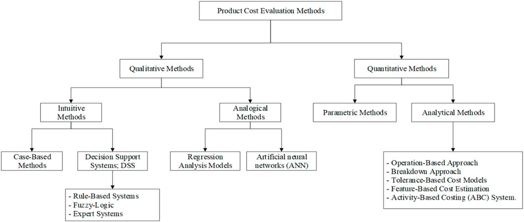
Figure 1. Classification of cost evaluation methods (Niazi et al., 2006; Ganorkar et al., 2017).

A number of literature reviews have been conducted on costing methods to study cost evaluation approaches. Wang (2007) presented the ANN with feature extraction to develop a cost estimation model for plastic products. This research compared the model learning cycle that selected the number of model learning cycles as 50,000 and reduced the projection area parameters. The mean absolute percentage error (MAPE) was decreased by 0.77%, and the cost percentage error was approximately ±2%. Che (2010) integrated particle swarm optimization (PSO) with the ANN and applied factor analysis to identify the peculiarity effect on the cost data of the product and mold for cost evaluation. The findings demonstrate that incorporating PSO with the back-propagation (BP) neural network improves the accuracy of cost identification for plastic injection molding by the cost percentage error (CPE) of parts, and mold costs are approximately ±0.4% and ±0.5%, respectively, which can lower the parameter settings of the BP neural network. Wang et al. (2013) applied PSO with the ANN to develop a cost estimation model of part costs in plastic products. The outcome of testing data for the CPE is approximately ±0.2% to ±1%. PSO can find optimal solutions and improve the convergence rate, which can achieve better accuracy. Tyagi et al. (2015) presented a product life-cycle cost identification mathematical model for a multigeneration manufacturing-based product that emphasizes market and technical risks. This study of mathematical models meets the need to obtain better accuracy and confidence in the prediction. Chan et al. (2018) developed a new cost identification method for additive manufacturing (AM) using big data analytics cyber manufacturing. This method applies feature extraction on elastic net (EN) regression with least absolute shrinkage and selection operator (LASSO) regression within each cluster. The outcome shows that the smaller cluster size affects the learning ability. The prediction error of LASSO is 85.16% less than that of EN regression, resulting in EN regression achieving better accuracy and efficiency than LASSO regression. Tosello et al. (2019) integrated AM in the injection molding process chain to optimize the value chain and manufacturing cost. The result indicates that using the AM inserts reduces lead times in product development by up to 66%, which can reduce the production time by at least 5 days and improve the manufacturing process. Ahn et al. (2020) developed a transportation cost evaluation model for prefabricated construction that adopted feature extraction of geo-fence-based large-scale GPS data with support vector regression (SVR) to predict transportation demand. The accuracy result of trailers and the duration are 86% and 88%, respectively, and the actual transportation cost decreased by approximately 14%, improving transportation cost evaluation efficiency. Tabkosai and Kengpol (2022) proposed a cost evaluation model for plastic products that integrated a 3D convolutional neural network (3D-CNN) with voxelization that can enhance excellent 3D voxel processing from a 3D model. The result proves that voxel 128³ resolutions are superior to voxel 64³ resolutions for both the part and mold. The accuracy of part and mold costs is approximately 97.55% and 92.66%, respectively.

According to previous research, various techniques are used in many different aspects of cost evaluation. However, a gap still exists in the method for reducing cost evaluation errors and a faster convergence rate for optimal solutions. Therefore, this research aims to apply the hybrid deep learning ability of the TSA to find optimization parameters of the ANN model to enhance learning capability and achieve higher accuracy to fill the gap mentioned above, which is unavailable in the literature.

2.2 Deep learning

Deep learning is a model that transfers the critical representation of self-learning characteristics at a multilayer ANN. Multi-dimensional scaling is a technique that automatically converts input attributes to output attributes (Emmert-Streib et al., 2020). Deep learning is the most popular method for information conversions due to its ability to handle information processing and instantly recognize an attribute of data at different levels of abstraction (Chien et al., 2020). The capability of deep learning models has surpassed that of widely used alignment-based methods with more outperformed in some circumstances (Mathieu et al., 2022).

Deep learning is a rising territory of machine learning (ML) and artificial intelligence (AI) that can have learning capabilities from data, which is a mainstream technology nowadays. Deep learning technology emerged from the ANN, which is used extensively in prediction, visual recognition, text analytics, cybersecurity, and other domains, as shown in Figure 2A (Sarker, 2021). A deep neural network typically consists of multilevel hidden layers, involving input and output layers. Figure 2B represents the typical neural network architecture compared with a deep neural network. The difference between a regular neural network and a deep learning network is the number of hidden layers. A typical neural network has one hidden layer, while a deep learning network has multiple hidden layers. The hidden nodes in each layer are processed from the input layer to the output layer (Xing and Du, 2018).

Figure 2

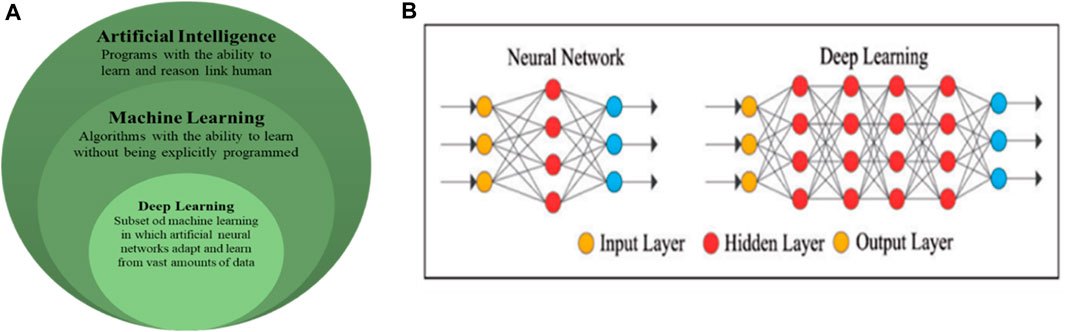
Figure 2. Relationship between deep learning (Sarker, 2021) and the typical architecture of a neural network and deep neural network (Xing and Du, 2018).

2.3 Tunicate swarm algorithm

TSA is an optimization technique for solving non-linear constrained problems, which draws inspiration from the survival behavior of tunicate swarms in the ocean’s depths. Among the simplest bio-inspired meta-heuristic optimization algorithms is the TSA. In over 74 benchmark problems, superiority over alternative optimization methods was demonstrated conclusively (Kaur et al., 2020). Fetouh and Elsayed (2020) mentioned that an effective and simple design encourages the consideration of implementing and enhancing this algorithm for the situation at hand. The TSA primarily emulates the swarming behavior and jet propulsions of marine tunicates that facilitate their navigation and foraging operations. A population of tunicates engages in swarming behavior in the TSA to locate the best food source; this behavior indicates the fitness function of the model. The tunicates in this swarm adjust their positions concerning the first optimal tunicates that are garnered and updated in each epoch. At the beginning of the TSA, a random initialization population of tunicates is generated within the allowed ranges of the control variables.

In the mathematical modeling for the first behavior of the tunicate, the jet propulsion must satisfy three essential conditions, namely, preventing collisions among the agent, approaching the position of the best agent, and maintaining proximity to the optimal solution (Sharma et al., 2020). Conversely, swarm behavior serves the purpose of notifying other seekers of their presence in order to locate the best optimal solution. The TSA starts with the tunicate populations being initialized randomly while considering the allowable bounds of the control variables. A^⃗ is a randomized vector to prevent conflicts between search agents in each tunicate. The new search agent position computation to avoid the collision between tunicates can be modeled as follows:

$\overrightarrow{\mathrm{A}}=\frac{\overrightarrow{\mathrm{G}}}{\overrightarrow{\mathrm{M}}},(1)$

$\overrightarrow{\mathrm{G}}={\mathrm{c}}_2+{\mathrm{c}}_3-\overrightarrow{\mathrm{F}},(2)$

$\overrightarrow{\mathrm{F}}=2\times {\mathrm{c}}_1,(3)$

where $\overrightarrow{\mathrm{A}}$ is a randomized vector for the initial tunicate, $\overrightarrow{\mathrm{G}}$ is the gravity force, $\overrightarrow{\mathrm{F}}$ is the movement of water in the ocean, and c₁, c₂, and c₃ are disorder grades with a range [0, 1].

The social force among search agents is the colony strength between the tunicates stored in a new vector $\overrightarrow{\mathrm{M}}$ that is determined as follows:

$\overrightarrow{\mathrm{M}}=\lfloor {\mathrm{P}}_{\min }+{\mathrm{c}}_1\times {\mathrm{P}}_{\max }-{\mathrm{P}}_{\min }\rfloor ,(4)$

where $\overrightarrow{\mathrm{M}}$ is the colony strength between the tunicates and P_min and P_max are the minimum speed and maximum speed of the tunicate to build social liaison, respectively. The variable P_min has a value of 1, and variable P_max has a value of 4.

In order to transition to the position of the optimal tunicate, one can prevent conflicts between tunicates and get closer to the optimal tunicates as follows:

$\overrightarrow{\text{PD}}=\left|\overrightarrow{\text{FS}}-r_{and}\times \overrightarrow{{\mathrm{P}}_{\mathrm{p}}}\left(\mathrm{x}\right)\right|,(5)$

where $\overrightarrow{\text{PD}}$ is the distance between the food source and tunicate, $\overrightarrow{\text{FS}}$ is the position of the food source (optimal fitness value), $\overrightarrow{{\mathrm{P}}_{\mathrm{p}}}\left(\mathrm{x}\right)$ is the position of the tunicate, and r_and is the disordered grade in space [0, 1].

The best tunicate can adjust its ranking to reflect the current state of affairs. The position of the food supply is related to this, as shown in the following equation:

$\overrightarrow{{\mathrm{P}}_{\mathrm{p}}}\left(\mathrm{x}\right)=\{\begin{array}{c}\overrightarrow{\text{FS}}+\overrightarrow{\mathrm{A}}\times \overrightarrow{\text{PD}},\text{if\hspace{0.17em}rand}\ge 0.5\\ \overrightarrow{\text{FS}}-\overrightarrow{\mathrm{A}}\times \overrightarrow{\text{PD}},\text{if\hspace{0.17em}rand\hspace{0.17em}}<0.5\end{array}.(6)$

In order to search for the optimum tunicate positions, the approach allows for keeping the optimal solutions and adjusting the others. The collective tunicate behavior can be expressed as follows:

$\overrightarrow{\mathrm{P}}\left(\mathrm{x}+1\right)=\frac{{\mathrm{P}}_{\mathrm{p}}\to \left(\mathrm{x}\right)+\overrightarrow{{\mathrm{P}}_{\mathrm{p}}}\left(\mathrm{x}+1\right)}{2\times {\mathrm{c}}_1}.(7)$

The final position inside a random region is determined by the position of the tunicate. The tunicate swarm algorithm can be summed up as follows.

- Parameters $\overrightarrow{\mathrm{A}}$, $\overrightarrow{\mathrm{G}}$, and $\overrightarrow{\mathrm{M}}$ prevent and encourage in a defined search space and escape conflict between tunicates.

- In order to use vector variations $\overrightarrow{\mathrm{A}}$, $\overrightarrow{\mathrm{G}}$, and $\overrightarrow{\mathrm{M}}$, it is anticipated that the investigation and exploitation method will obtain a greater value.

- The collective behavior exhibited by the TSA is comparable to the behavior of tunicate colonies and jet propulsion.

Many research studies apply the TSA. Aribowo et al. (2020) proposed the TSA to improve the performance of the feed-forward neural network (FFNN) that used optimization weight to obtain better output results for the adaptive power system stabilizer parameter. The outcome demonstrates that the TSA can adjust parameters and outperform the outputs of alternative approaches. Kaur et al. (2020) proposed a new bio-inspired metaheuristic optimization method that studies the TSA to analyze sensitivity, convergence, and scalability analysis with the ANOVA test. The outcome shows that the TSA can obtain a better optimal solution than other algorithms, which can solve problems with unknown search space. Fetouh and Elsayed (2020) applied an improved TSA with distribution network reconfiguration (DNR) for optimal control and operation of capacitor banks (CBs) and distributed generators (DGs) that can achieve the optimal solution and outperforms the other algorithms in the literature. The benefit of research can reduce power losses by approximately 96.97%. The results show that the TSA can enhance performance for fully automated distribution networks. Sharma et al. (2020) applied the TSA to evaluate the optimal solution of the unknown parameters for the photovoltaic module under standard temperature conditions. The RMSE results indicate that the optimization of the TSA is superior to other algorithms and yields an excellent convergence rate. Nguyen et al. (2020) designed the TSA for the Internet of Health Things (IoHT) to protect medical image data in a cloud server using energy-efficient lightweight encryption and fog computing. The efficiency of IoHT combined the peak signal-to-noise ratio (PSNR) with the number of pixel changing rate (NPCR), resulting in improved accuracy of medical reports and fewer computations on a cloud server. Houssein et al. (2021) combined a TSA with a local escaping operator (LEO) to improve the convergence rate and local search performance of swarm agents for image segmentation. The performance of TSA-LEO achieves optimal solutions and accelerates the convergence rate with better efficiency than other metaheuristic algorithms. According to the previous research mentioned above, it was found that the TSA can solve unknown search space and enhance the rapid convergence rate. Although the TSA is widely used in optimal solutions to solve unknown parameters, no evidence has been found to develop the TSA in the cost evaluation of complicated surface products. Therefore, this research aims to apply the TSA to optimize initial weight to improve the performance of the ANN that can achieve faster-to-convergent optimal solutions and higher accuracy in the cost evaluation model.

2.4 Artificial neural network

The ANN involves computations and mathematical models that include diverse processing components comparable with human brain processing, which obtain inputs and transfer output based upon their predetermined activation functions (Kengpol and Neungrit, 2014). The most widely used ANN for a wide range of issues is based upon a supervised procedure that employs multilayer perceptrons (MLPs) with BP learning algorithms. The ANN architecture comprises an input layer as the neuron is the input variable to problem solving. The different values are distinct in each characteristic, causing attribute disorder and influencing the obtained findings. Therefore, normalization is essential to convert data to a single based upon each attribute (Henderi, 2021). The hidden layer is responsible for conveying the weighted connections, which are indicated as weights in the computation process of the input layer and transferred to the output layer through the hidden layer. The weight value is important to the propagation of the network model. The magnitude of the signal that traverses from the hidden layer to the output layer is determined by the weight connected between them. The number of independent variables used to predict the target value of output in the model is directly proportional to the number of neurons in the input layer. The number of hidden layers and neurons is determined by the complication of the model, which describes the computation in the methodology section. The forward propagation is the initial process consisting of weights and biases to minimize the error for the neural network training of the input layer and processing transferred in backward propagation of the output layer. Figure 3 depicts the processing of necessary neurons at their hidden nodes.

Figure 3

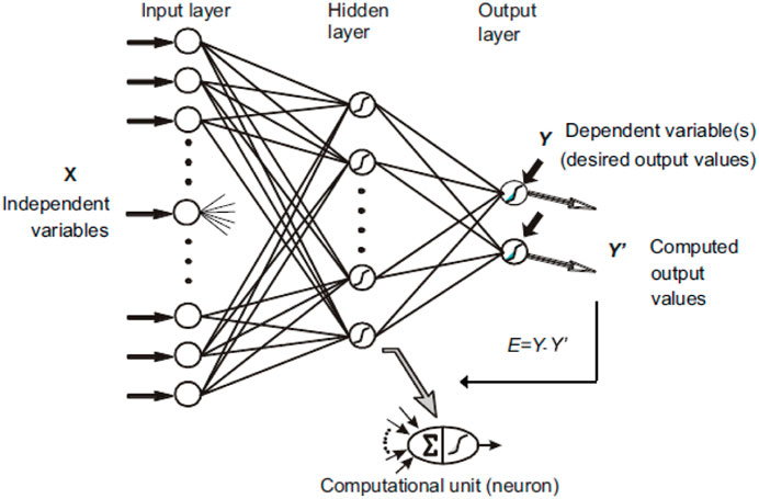
Figure 3. Architecture of the artificial neural network (ANN) (Henderi, 2021).

The neuron receives the hidden nodes from each input. Then, the activation function is used to compute the optimal solution in the output model through the summation of the input node values multiplied by their assigned weights. The mathematical function of the ANN can be explained as follows (Kengpol and Neungrit, 2014).

In order to define the number of hidden layers for large features and achieve optimal solutions, Equation 8 presents the calculation of the number of hidden layers, developed by the authors, which is usually estimated through trial and error tests to reduce cost errors in the development model.

$\text{Nh}=\sqrt{\text{Ns}}/\left(\mathrm{I}+\mathrm{O}\right),(8)$

where Nh is the number of hidden layers, Ns is the number of samples, I is the number of the input, and O is the number of the output.

The output result can be determined from Eqs (9) and (10):

$y_j=f\left(\sum w_{ij}{x}_i+b_j\right)=f\left(v\right),(9)$

$v=\sum w_{ij}{x}_i+b_j,(10)$

where y_j is the activation values, f is the activation function, v is the summation of weight in each input, w_ij is the weight variables of input neurons i to output neurons j, x_i is the input variable, and b_j is the bias variable.

The activation function applied the sigmoid function that is suitable for non-linear problems to predict the result as follows in Equation 11:

${\mathrm{f}}_{\mathrm{z}}=\frac{1}{1+{\exp }^{-\mathrm{z}}},(11)$

where f_z is the fitness function of the variable.

Several research studies propose an ANN. Juszczyk et al. (2018) suggested the capacity to receive information in the automated training process of neural networks and apply it to calculate sports field construction expenses. Kengpol et al. (2018) explained that the capability of the ANN has the advantage of predicting data that have never been seen before in the learning process. The ANN is one of the techniques used to solve non-linear problems, which necessitates computing intelligence. The BP algorithm is a supervised learning technique that accurately recognizes patterns and predictions (Kengpol and Klunngien, 2019). Elhoone et al. (2020) used an expert system based upon ANNs in conjunction with the Internet of Things (IoTs) to determine the most efficient AM procedures for a wide range of product development in a cyber network-processable environment. Moreover, the ANN can classify and detect complex non-linear problems without using complicated mathematics that achieves prediction accuracy (Wong et al., 2022). Predictive modeling is essential to research that can be studied and improved using the ANN as demonstrated by the success of these studies. However, no evidence has been encountered to propose a hybrid deep learning TSA with an ANN for the cost evaluation of complicated surface products in the plastic injection industry. Therefore, the purpose of this study is to provide a new approach to fill the gap mentioned above.

2.5 Research methodology

The cost evaluation model in the plastic injection industry applies a hybrid deep learning methodology using a TSA with an ANN for complicated surface products. Figure 4 represents the method that entails feature-based extraction of complicated surface products using the TSA to construct the initial weight into the ANN learning process, which is described in more detail as follows:

Figure 4

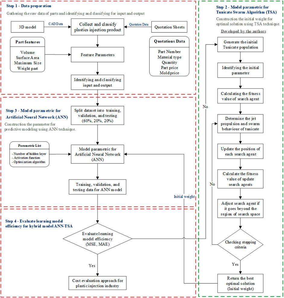
Figure 4. Cost evaluation of the hybrid tunicate swarm algorithm (TSA) with the ANN (developed by the authors).

Step 1: Data preparation.

1. Data collection: The data preparation method starts with collecting and categorizing raw data from the 3D-model complicated surface products and quotation data. The product design varies in appearance in application usage. This study emphasizes complicated surface products of electronic parts, automotive parts, packaging parts, and medical parts for developing a cost evaluation model. An example of a complicated surface part is given in Figure 5.

2. Feature parameters: The plastic injection industry has more advanced technology in product design and production processes that result in plastic products having a more complex appearance. The designer uses CAD/CAM technology to create a 3D model of specific products in the design stage. This method extracts feature-based parameters of a 3D model for complicated surface products as input variables into the ANN model. The input variables are quantitative parameters that require converting all non-calculable data into calculable values. The input variables involve the maximum size of the product in the X, Y, and Z axes, the surface part, the weight part, and the volume of the product, as shown in Figure 5. In this study, the focus is on the material polypropylene (PP) because of its wide usage and its most excellent feasibility for a high market value. The key factors in calculating the immemorial plastic injection cost evaluation include material costs, manufacturing costs, and molding costs (Wang, 2007). Table 1 represents the distinctions between standard cost evaluation approaches and our novel cost evaluation model in bringing feature parameters to use as a replacement for various factors.

Figure 5

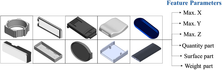
Figure 5. Example of complicated surface products and parameter features.

Table 1

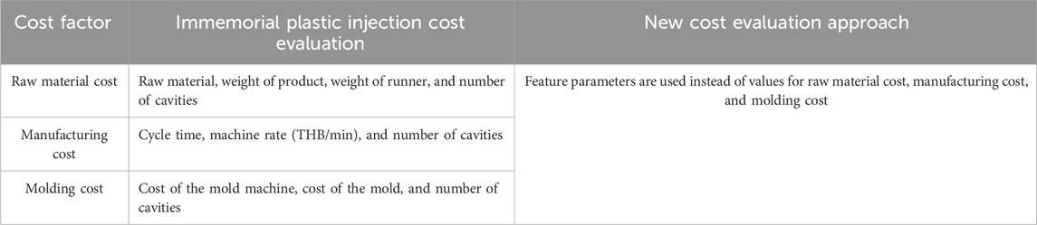
Table 1. Factor comparison of the traditional and new cost evaluation approaches.

Step 2: Model parametric for the TSA.

This section proposes a new method for constructing the initial weight from the TSA technique applied to an ANN that has more capabilities than other swarm intelligence algorithms to find the faster optimal solution. Therefore, this study enhances the learning model and achieves better accuracy. The step and flowchart are given in Figure 6. The steps proposed for the TSA methodology are given below.

Figure 6

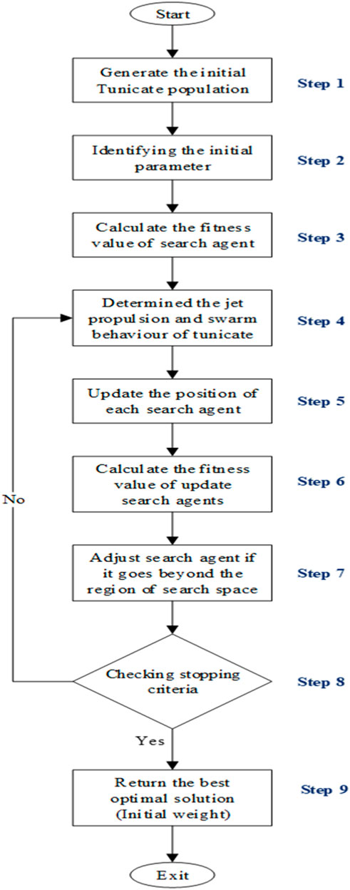
Figure 6. Flowchart of the proposed TSA (Arabali et al., 2022).

Step 1: Generating the initial tunicate population. The TSA produces the initial population of tunicates $\overrightarrow{{\mathrm{P}}_{\mathrm{p}}}\left(\mathrm{x}\right)$, which is equal to the number of nodes that are processed in the ANN model. The TSA process commences by randomly initializing the tunicate population, which is defined within the value range of 0–1, and the total population consists of 50,370 tunicates that consider the allowable limits of the control variables under the condition of the model learning ANN.

Step 2: Identifying the initial parameter. Table 2 represents the parameter setting of the TSA that is to define the initial parameters to be used in the next step of calculation, including c₁, c₂, c₃, and r_and, that specify random parameters in the range from 0 to 1 [0,1]. The constant value assigned to P_min is 1, and P_max is defined as 4. The max iteration is determined at 1,000 iterations.

Table 2

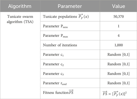
Table 2. Parameter setting of the tunicate swarm algorithm (TSA).

Step 3: Calculating the fitness value. The fitness function was obtained from the start of the calculation from the colony strength between the tunicates in vector and M ^⃗ from Equation 4. Then, the movement of water is calculated in the ocean $\overrightarrow{\mathrm{F}}$ from Equation 3. Then, the gravity force $\overrightarrow{\mathrm{G}}$ is determined from Equation 2, and the new search agent position $\overrightarrow{\mathrm{A}}$ is computed from Equation 1. Finally, the position of the food source that is represented by the best tunicate position (Fs) is computed to obtain the optimal fitness value. The optimal function is $\overrightarrow{\text{FS}}$ = ${\left[\overrightarrow{{\mathrm{P}}_{\mathrm{p}}}\left(\mathrm{x}\right)\right]}^2$ in each tunicate.

Step 4: Determining the jet propulsion and swarm behavior of the tunicate. In order to transition to the position of the optimal tunicate for evaluating the best search agent within the available search space after computing the fitness value, the distance between the food source and the tunicate $\overrightarrow{\text{PD}}$ is calculated from Equation 5. The best tunicate can adjust its ranking to reflect the current state of affairs. The position of the search agent is determined from Equation 6 for verifying the boundary condition of the position of the tunicate $\overrightarrow{{\mathrm{P}}_{\mathrm{p}}}\left(\mathrm{x}\right)$.

Step 5: Updating the position of each search agent: In order to adjust the locations of the tunicates and update the positions of the search agents, the new positions of the tunicates are determined by data concerning the optimal position of the tunicates and the social interactions among the tunicates in Equation 7.

Step 6: Calculating the fitness value of updated search agents. The fitness value of the updated search agents from Equation 7 that are out of bounds in the regulative search space are evaluated by the nearest limit that should be chosen.

Step 7: Adjusting the search agent if it goes beyond the region of search space. The fitness function associated with each new location search is computed, and the tunicate position that is the fitness value is updated by adjusting the search agent if it is better than the previous optimal solution. Then, the position of the tunicate $\overrightarrow{{\mathrm{P}}_{\mathrm{p}}}\left(\mathrm{x}\right)$ is updated.

Step 8: Checking stopping criteria. Termination requirements should be verified. The method continues iterating until the algorithm terminates, at which point the iteration count is incremented by one. Stylianos et al. (2022) proposed optimization iterations to enhance the performance of carbon nanocomposite reinforcement in cement-based materials. This method compared the number of iterations between 20 iterations, 200 iterations, and 1,000 iterations. The results show that a maximum number of 1,000 iterations achieved excellent accuracy at approximately 99.99%. Therefore, a maximum number of 1,000 iterations are applied in this research to repeat steps 5–8 to obtain great results.

Step 9: Returning the best optimal solution (initial weight). The output of the optimal solution acquired from the TSA is transferred to process learning for the initial weight of the ANN model.

In the process, the TSA yields the best optimal solution as the initial weight to use as the default weight in the feed forward of the ANN model, which is clarified in step 3 in the following order.

Step 3: Model parametric for the ANN

According to the literature review, this segment proposes the new hybrid TSA-ANN for the cost evaluation of complicated surface products. The learning process of the ANN uses a feature extraction of complicated surface products and obtains the initial weight from the output of the TSA that is applied to the FFNN. In order to minimize prediction errors, this section suggests a training and validation model configuration for an architecture that would evaluate the cost of complicated surface products in the plastic injection industry, which is explained in more detail as follows.

1. The dataset is split into training, validation, and testing sets (60%, 20%, and 20%, respectively): The most crucial aspect of learning process development is splitting data for model validation (Xu and Goodacre, 2018). Hemelings et al. (2021) adopted the splitting data process, which is significant in the learning model. This research divided the dataset into three groups for model development, namely, 60% of the training datasets, 20% of the validation datasets, and 20% of the testing datasets.

2. Model parametric for the ANN: This segment applies the feature parameters of 3D-model complicated surface products as the input variable of the ANN. The initial weight of the ANN was obtained from the TSA technique in the result of step 9 in Figure 6. The parametric list was obtained from trial and error to minimize errors by splitting datasets for training, validation, and testing datasets to find the optimal solution for the ANN model. The hybrid TSA-ANN model architecture in this research is given in Figure 7.

Figure 7

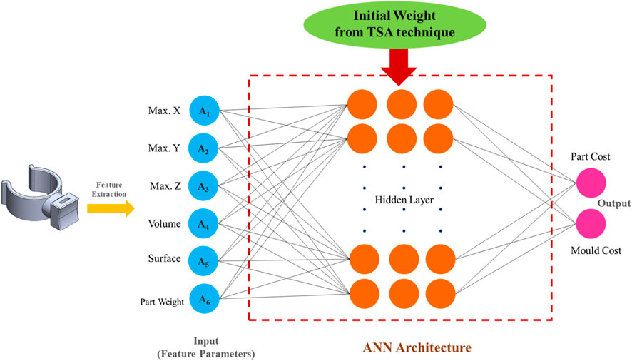
Figure 7. Hybrid deep learning TSA with ANN model architecture.

In the starting model development of the ANN, the input is denoted by the first layer, which consists of the input variable obtained from the feature extraction of complicated surface products as six nodes. The input variables involve the maximum size of the product in the X, Y, and Z axes, the surface part, the weight part, and the volume of the product. Due to the different value ranges for each attribute, normalization is necessary to convert the data to a similar scale (Henderi, 2021). In order to construct the equation for normalization between 0 and 1, the minimum value of the variable to be normalized is initially subtracted. Following the subtraction of the minimum value from the maximum value, the resulting value is divided by the minimum value, as shown in Equation 12:

${\mathrm{X}}_{\text{norm}}=\left({\mathrm{X}}_{\mathrm{i}}-{\mathrm{X}}_{\min }\right)/\left({\mathrm{X}}_{\max }-{\mathrm{X}}_{\min }\right),(12)$

where X_norm is the new normalization data, X_i is the set of observed values of X, X_max is the maximum value in X, and X_min is the minimum value in X.

Alwosheel et al. (2018) suggested that the minimum number of samples suitable for the ANN is 50 times the number of variables. The learning process of the ANN can achieve satisfactory performance, with a sample size of 2,000 (Alwosheel et al., 2018). However, the sample size according to the above definition for 6 input variables in this research is approximately 6 × 50 = 300. In order to obtain excellent learning capability of the ANN, the number of samples is specified as 2,000. The number of inputs is six variables, and the number of outputs is two target values for the calculation mentioned in Equation 8. Thus, the number of hidden layers is [$\sqrt{\mathrm{2,000}}$/(6 + 2)] = 5.59, so inference uses 6 hidden layers for this research.

The optimal number of hidden nodes is determined using the number of nodes with the least amount of error to validate the learning model. Table 3 demonstrates the model summary of the ANN, and the input layer has 6 hidden nodes for variables, in which the output shape is (none, 6). Next, the hidden layers 1, 2, and 3 define the number of hidden nodes as 64, and the output shape is (none, 64). Then, the hidden layers 4, 5, and 6 define the number of hidden nodes as 128, and the output shape is (none, 128). The final layer is the output layer of the part, and the mold that defines 1 hidden node for the target value as the output shape is (none, 1). The “None” in the output shape means a dynamic dimension of a batch without being pre-determined that is flexible to adjust the batch size by extrapolating shape from the context in each layer. The “Param #” column represents the number of parameters that are multiplied between the weight of the previous layer and the current layer, plus with bias, which can be explained as follows.

Table 3

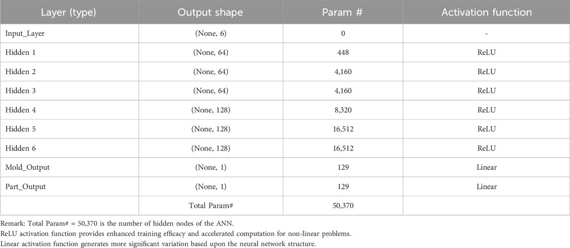
Table 3. Model summary of artificial neural network (ANN) architecture.

Hidden 1: The number of Param # in hidden 1 is 448, which is obtained as 6 (input variables) multiplied by 64 (hidden node in hidden 1) and plus by 64 (bias value in hidden 1).

Hidden 2: The number of Param # in hidden 2 is 4,160, which is obtained as 64 (hidden node in hidden 1) multiplied by 64 (hidden node in hidden 2) and plus by 64 (bias value in hidden 2).

Hidden 3: The number of Param # in hidden 3 is 4,160, which is obtained as 64 (hidden node in hidden 2) multiplied by 64 (hidden node in hidden 3) and plus by 64 (bias value in hidden 3).

Hidden 4: The number of Param # in hidden 4 is 8,320, which is obtained as 64 (hidden node in hidden 3) multiplied by 128 (hidden node in hidden 4) and plus by 128 (bias value in hidden 4).

Hidden 5: The number of Param # in hidden 5 is 16,512, which is obtained as 128 (hidden node in hidden 4) multiplied by 128 (hidden node in hidden 5) and plus by 128 (bias value in hidden 5).

Hidden 6: The number of Param # in hidden 6 is 16,512, which is obtained as 128 (hidden node in hidden 5) multiplied by 128 (hidden node in hidden 6) and plus by 128 (bias value in hidden 6).

Mold output: The number of Param # in the mold output layer is 129, which is obtained as 1 (target value of the mold cost) multiplied by 128 (hidden node in hidden 6) and plus by 1 (bias value in mold output).

Part output: The number of Param # in part output layer is 129, which is obtained as 1 (target value of part cost) multiplied by 128 (hidden node in hidden 6) and plus by 1 (bias value in part output).

Wibawa et al. (2018) used the rectifier linear unit (ReLU) activation function for the learning model to identify abnormal heart rhythms, which provides enhanced training efficacy and accelerated computation. Furthermore, the model optimization incorporated the Adam approach for weight adjustment, which yielded outstanding outcomes. Consequently, the ReLU activation function is implemented in the hidden layer of each dense that can apply the Adam approach to complicated functional mappings for non-linear problems to optimize the cost evaluation model, as shown in Equation 13. Feng and Lu (2019) proposed a straight-line equation as an identity function to the linear activation function that maintains a constant value that suits the default activation when developing a multilayer perceptron. The linear activation function as specified for the output layer in this study is denoted by Equation 14.

$\text{ReLU\hspace{0.17em}Activation\hspace{0.17em}Function};\mathrm{f}\left(x_i\right)=\left\{\begin{array}{c}0\text{\hspace{0.5em}for\hspace{0.17em}}{x}_i\le 0\\ \mathrm{x}\text{\hspace{0.5em}for\hspace{0.17em}}{x}_i>0\end{array}\right.=\max \left\{0,\mathrm{x}\right\},(13)$

where x_i is the input for each neuron of function f on i, the output is 0 when x_i< 0, and the output is x when x_i>0.

$\text{Linear\hspace{0.17em}Activation\hspace{0.17em}function};\mathrm{f}\left({\mathrm{x}}_{\mathrm{i}}\right)={\text{kx}}_{\mathrm{i}},(14)$

where x_i is the input for each neuron of function f on i and k is a constant value.

3. Training, validation, and testing data for the ANN model: The accuracy of training datasets is being able to learn the correct patterns. The validation datasets aid in precisely fine-tuning the learning model, and the testing datasets furnish reliable metrics that instill confidence in the deployment of deep learning. This process uses the trial and error method to minimize errors in each dataset, which aims to achieve better accuracy and faster convergence for the learning model of the ANN. The optimal solution to minimize errors is to evaluate the efficiency of the learning model using error metrics to compare the predicted costs with the actual costs, which are described in more detail in the next section.

Step 4: The learning model efficiency is evaluated for the hybrid deep learning TSA-ANN.

According to the information mentioned above, error metrics are employed to assess the performance of the learning model of training, validation, and testing datasets that compare the predicted costs with the actual costs. The outcomes of these evaluations are significantly impacted by the implementation of deep learning techniques. Dessain (2021) suggested that the mean square error (MSE) and mean absolute error (MAE) are commonly used indicators for assessing the effectiveness of cost evaluation models and achieving excellent results. Consequently, the MSE and MAE are applied in this research to evaluate learning model efficiency for the hybrid deep learning TSA-ANN, which can be formulated using Equations (15) and (16).

$\text{Mean\hspace{0.17em}square\hspace{0.17em}error};\text{\hspace{0.17em}MSE}=\frac{{\displaystyle {\sum }_{\mathrm{i}=1}^{\mathrm{n}}}{\left(\mathrm{A}{\mathrm{v}}_{\mathrm{i}}-\mathrm{E}{\mathrm{v}}_{\mathrm{i}}\right)}^2}{\mathrm{n}-1},(15)$

$\text{Mean\hspace{0.17em}absolute\hspace{0.17em}error};\text{\hspace{0.17em}MAE}=\frac{{\displaystyle {\sum }_{\mathrm{i}=1}^{\mathrm{n}}}\left|\mathrm{A}{\mathrm{v}}_{\mathrm{i}}-\mathrm{E}{\mathrm{v}}_{\mathrm{i}}\right|}{\mathrm{n}},(16)$

where Av_i is the actual observed value, Ev_i is the corresponding predicted value, and n is the number of observations.

The efficiency of learning evaluation is considered by error metrics of the MSE and MAE. The parametric list configuration of the ANN model is fine-tuning to minimize errors. If the error metrics show an unstable trend and still have high errors, it is essential to repeat and adjust the parametric lists. On the other hand, the error metrics trend is stable and obtains excellent accuracy, resulting in achieving the best model for cost evaluation in the plastic injection industry. The results of learning the new hybrid TSA-ANN model are illustrated in Section 3.

3 Results and discussion

This section outlines the methods utilized for cost evaluation in the plastic injection industry. The suggested method for evaluating the cost of the hybrid deep learning TSA-ANN involves the process of the ANN obtaining the initial weight from the TSA to develop a cost evaluation model. The error metrics used the MSE and MAE to assess the efficiency of the cost prediction in the context of part and mold costs. The performance comparison of learning evaluation models for the ANN and a new hybrid deep learning TSA-ANN is shown in Table 4.

Table 4

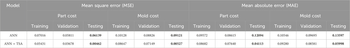
Table 4. Performance comparison of the artificial neural network (ANN) and a new hybrid deep learning tunicate swarm algorithm (TSA)–ANN.

The MSE of testing datasets for the ANN model in terms of part costs is approximately 0.06139 and mold cost is approximately 0.09121. The MSE for the new hybrid deep learning TSA-ANN of part and mold costs is approximately 0.00462 and 0.00527, respectively. The MAE of the ANN is approximately 0.12094 for part costs and 0.13597 for mold costs. The new hybrid deep learning TSA-ANN-obtained MAE of part and mold costs is approximately 0.04113 and 0.05998, respectively. The outcome indicates that the new hybrid deep learning TSA-ANN has fewer error than the ANN for both MSE and MAE. As a result, the convergence behavior of the model development for the new hybrid deep learning TSA-ANN is superior to that of the ANN.

Figures 8A–D depict the convergence behavior for the resultant of the MSE and MAE in both part and mold costs between the ANN and TSA-ANN. The curve of the ANN and TSA-ANN shows a likewise pattern that compares the training datasets with validation datasets. Figure 8A represents the learning rate of the MSE in terms of part costs, which initially exhibits a faster convergence and gradually decreases over the course of the subsequent 90 iterations for the ANN and 10 iterations for the TSA-ANN. The resultant of the TSA-ANN for the training rate is approximately 0.05601 and for the validation rate is approximately 0.03943. Then, the trend decreases until it stabilizes in 250 iterations at the intermediate trend and halts at the stable point where the learning trend has stabilized, which occurs in 500 iterations in the learning process where the training rate is at 0.05431 and the validation rate is at 0.03678. The MAE in the context of part costs shown in Figure 8B suggested astute convergence characteristics, despite the initial knobby nature of the path. The beginning stage appears to rapidly converge and move downward until it is at a stable point at 90 iterations for the ANN and 10 iterations for the TSA-ANN. The training rate of the TSA-ANN is approximately 0.07575, and the validation rate is approximately 0.06903, approaching the desired target value and terminating the runtime in 500 iterations at roughly 0.08682 for the training rate and 0.07640 for the validation rate.

Figure 8

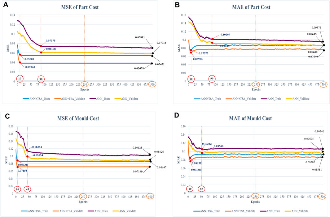
Figure 8. Learning curve comparison of the ANN and hybrid deep learning ANN with the TSA.

According to the outcome of the preceding discussion, the convergence behavior of the mold cost has a similar pattern to that of the part cost that compares two line plots between the training and validation datasets. The MSE of mold cost demonstrated a rapid decline trend, as shown in Figure 8C, within 45 iterations for the ANN and 10 iterations for the TSA-ANN. The result of the training rate and validation rate with convergence is approximately 0.08658 and 0.07158, respectively. The termination runtime of the training dataset is approximately 0.08647, and the validation dataset is approximately 0.07149 over the course of 500 iterations. The learning curve of the MAE is shown in Figure 8D, which initially demonstrates a faster convergence and steadily decreases within 55 iterations for the ANN and 10 iterations for the TSA-ANN. The runtime stops at the stable point throughout 500 iterations, with the training and validation rates of 0.09280 and 0.08581, respectively. Therefore, the outcome of the MSE and MAE for the part cost illustrates higher capability than that for the mold cost. In addition, the convergence behavior toward the termination runtime of the TSA-ANN results in a faster convergence than the ANN.

The comparison of the accuracy of the TSA-ANN for evaluating the part and mold costs of complicated surface products is shown in Figure 9. The accuracy of part cost is represented in green charts at approximately 92.44% for the ANN and 96.66% for the TSA-ANN. The accuracy of mold cost is indicated in blue charts at approximately 90.22% for the ANN and 93.75% for the TSA-ANN. Therefore, the new hybrid deep learning TSA-ANN model of testing datasets appears that the TSA can improve the learning ability of the ANN and obtain better accuracy than the ANN.

Figure 9

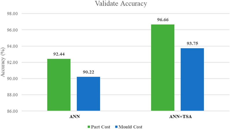
Figure 9. Accuracy comparison of the ANN and TSA-ANN on part and mold cost.

The results of the learning model above illustrate the methodology presented in the cost evaluation approach that combines the ANN with the TSA and has excellent efficiency. In terms of applications, the proposed cost evaluation model is verified using the cost percentage error (CPE) with complicated surface products of the new hybrid deep learning TSA-ANN. The computing equation is as follows (Juszczyk et al., 2018):

$\text{CPE}=\frac{\left({\text{Yp}}_{\mathrm{i}}-{\text{Ya}}_{\mathrm{i}}\right)}{{\text{Ya}}_{\mathrm{i}}}\times 100,(17)$

where Yp_i is the prediction cost of sample i and Ya_i is the actual cost of sample i.

The predicted cost evaluation of the new hybrid deep learning TSA-ANN in terms of part and mold costs is shown in Table 5. The first column of this table is the number of samples. The second column contains 20 samples, all of which have complicated surface products. The third column shows the cost prediction for the part cost, and the prediction of the mold cost is indicated in the final column.

Table 5

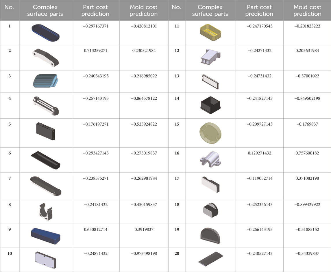
Table 5. Complicated surface products with the prediction of part and mold costs.

The CPE facilitates sight in errors in cost evaluation. Figure 10 depicts the CPE of the complicated surface products in both part and mold costs. The green charts obtained a CPE of approximately ±0.40% of 13 parts, accounting for 65% of the sample parts for mold cost. The violet charts obtained a CPE of approximately ±0.40% of 14 parts, accounting for 70% of the sample parts for part cost. The result illustrates cost evaluation errors of less than 1% in both part and mold costs, which can achieve a higher accuracy for complicated surface products. The validation and testing data of sample parts can achieve excellent performance for complicated surface products and can be applied to simple surface products that can reduce the complicatedness of cost evaluation in the plastic injection industry as well.

Figure 10

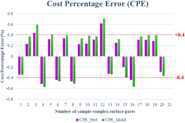
Figure 10. Cost percentage error (CPE) of the hybrid deep learning TSA-ANN on part and mold costs.

4 Conclusion and recommendations

The complexity of the plastic parts and manufacturing data resulted in a long data waiting time and inaccurate cost evaluation. Traditional cost evaluation approaches are limited and outdated, which are inappropriate practical operations to reduce cost evaluation mistakes for complicated surface products and decision-maker variability. However, a gap still exists in the method for decreasing cost evaluation errors and increasing the convergence rate for faster optimal solutions in model development. Therefore, the aim of this research is to apply a cost evaluation approach that combines hybrid deep learning of the TSA with the ANN for the cost evaluation of complicated surface products in the plastic injection industry to achieve a faster convergence rate for optimal solutions and higher accuracy.

The value of this research is the higher accuracy of the new hybrid deep learning TSA-ANN that can generate much less CPE of the complicated surface part in both part and mold costs. Although research has been conducted on cost estimation in plastic injection, these consider only cost estimation in the simple surface product. Wang (2007) obtained a CPE of approximately ±2% for part cost. Che (2010) attained a CPE of part and mold costs of approximately ±0.4% and ±0.5%, respectively, and Wang et al. (2013) achieved a CPE of approximately ±0.2% to ±1% for part costs. The outcome of the new hybrid deep learning TSA-ANN can achieve excellent efficiency for complicated surface products with the CPE of approximately ±0.40% of 13 parts, accounting for 65% of the sample parts for mold cost and approximately ±0.40% of 14 parts, accounting for 70% of the sample parts for part cost.

The new approaches reduce cost evaluation errors for complicated surface products in the plastic injection industry. The methodology entails TSA to construct the initial weight into the learning process of the ANN using the jet propulsion and swarm behavior function to achieve the best tunicates that can generate faster-to-convergent optimal solutions. The ANN applied feature-based extraction of complicated surface products as input variables for developing the model. The number of hidden layers obtained from calculation uses the value of six for this research. A fully connected multilayer neural network is an essential part of deep learning. The result shows that the new hybrid deep learning TSA-ANN provides a more accurate cost evaluation than using the ANN only. The TSA has the function to minimize errors to find the best tunicate that can be used as the default weight in the feed forward of the ANN and eventually achieve a faster-to-convergent optimal solution.

The benefit of this research is to establish a higher accuracy cost evaluation of complicated surface products. Moreover, the ANN can generate self-learning ability for non-linear problems, and the TSA can save time to find the optimal solution. Thus, the new hybrid deep learning TSA-ANN can minimize errors and decrease the complicatedness of cost evaluation.

The contribution of this research is to integrate a new hybrid deep learning application of the TSA with the ANN that fills a gap in the literature and proposes a method for calculating the number of hidden layers for reducing cost evaluation errors and obtaining a faster convergence rate, which is unavailable in the literature. The advantage of this study is that the new hybrid deep learning TSA-ANN achieves higher accuracy and is able to quote pricing rapidly for complicated surface products. This means a reduction in cost evaluation complexity in the plastic injection industry.

The limitations of this research are that a 3D-model file for complicated surface products is enormously needed, which can lead to higher computation, which can be time-consuming. In addition, the processing of the 3D-model data seeks high graphics processing unit (GPU) processors.

For future study, this new hybrid deep learning TSA-ANN cost evaluation model can also be applied to other industries, and the faster-to-convergent optimal solution should be enhanced further to the full extent.

Data availability statement

The raw data supporting the conclusion of this article will be made available by the authors, without undue reservation.

Author contributions

AK: writing–original draft and writing–review and editing. PT: writing–original draft and writing–review and editing.

Funding

The author(s) declare that no financial support was received for the research, authorship, and/or publication of this article.

Acknowledgments

This research would not have been successful without the exceptional support of my professor. The authors acknowledge the preciously provided knowledge, expertise, and exacting attention to detail, which is an inspiration and keeps our works on track. The authors acknowledge King Mongkut’s University of Technology North Bangkok (KMUTNB) for supporting the knowledge and companies that provide supporting data, the identities of which are protected by a confidentiality agreement.

Conflict of interest

The authors declare that the research was conducted in the absence of any commercial or financial relationships that could be construed as a potential conflict of interest.

Publisher’s note

All claims expressed in this article are solely those of the authors and do not necessarily represent those of their affiliated organizations, or those of the publisher, the editors, and the reviewers. Any product that may be evaluated in this article, or claim that may be made by its manufacturer, is not guaranteed or endorsed by the publisher.

References

Ahn, J., Han, S., and Al-Hussein, M. (2020). Improvement of transportation cost estimation for prefabricated construction using geo-fence-based large-scale GPS data feature extraction and support vector regression. Adv. Eng. Inf. 43, 101012. doi:10.1016/j.aei.2019.101012

CrossRef Full Text | Google Scholar

Arabali, A., Khajehzadeh, M., Keawsawasvong, S., Mohammed, A. H., and Khan, B. (2022). An adaptive tunicate swarm algorithm for optimization of shallow foundation. IEEE Access 10, 39204–39219. doi:10.1109/ACCESS.2022.3164734

CrossRef Full Text | Google Scholar

Chan, S. L., Lu, Y., and Wang, Y. (2018). Data-driven cost estimation for additive manufacturing in cyber manufacturing. J. Manuf. Syst. 46, 115–126. doi:10.1016/j.jmsy.2017.12.001

CrossRef Full Text | Google Scholar

Chang, K.-H. (2015). “Product cost estimating,” in e-Design (Amsterdam, Netherlands: Elsevier Inc), 787–844. doi:10.1016/B978-0-12-382038-9.00015-6

CrossRef Full Text | Google Scholar

Che, Z. H. (2010). PSO-based back-propagation artificial neural network for product and mold cost estimation of plastic injection molding. Comput. Industrial Eng. 58 (4), 625–637. doi:10.1016/j.cie.2010.01.004

CrossRef Full Text | Google Scholar

Chien, C.-F., Dauzère-Pérès, S., Huh, W., Jang, Y. J., and Morrison, J. (2020). Artificial intelligence in manufacturing and logistics systems: algorithms, applications, and case studies. Int. J. Prod. Res. 58, 2730–2731. doi:10.1080/00207543.2020.1752488

CrossRef Full Text | Google Scholar

Dessain, J. (2021). Machine learning models predicting returns: why most popular performance metrics are misleading and proposal for an efficient metric. Available at: https://ssrn.com/abstract=3927058or10.2139/ssrn.3927058.

Google Scholar

Elhoone, H., Zhang, T., Anwar, M., and Desai, S. (2020). Cyber-based design for additive manufacturing using artificial neural networks for Industry 4.0. Int. J. Prod. Res. 58 (9), 2841–2861. doi:10.1080/00207543.2019.1671627

CrossRef Full Text | Google Scholar

Emmert-Streib, F., Yang, Z., Feng, H., Tripathi, S., and Dehmer, M. (2020). An introductory review of deep learning for prediction models with big data. Front. Artif. Intell. 3, 4. PMID: 33733124; PMCID: PMC7861305. doi:10.3389/frai.2020.00004

PubMed Abstract | CrossRef Full Text | Google Scholar

Feng, J., and Lu, S. (2019). Performance analysis of various activation functions in artificial neural networks. J. Phys. Conf. Ser. 1237, 022030. doi:10.1088/17426596/1237/2/022030

CrossRef Full Text | Google Scholar

Fetouh, T., and Elsayed, A. M. (2020). Optimal control and operation of fully automated distribution networks using improved tunicate swarm intelligent algorithm. IEEE Access 8, 129689–129708. doi:10.1109/ACCESS.2020.3009113

CrossRef Full Text | Google Scholar

Ganorkar, A. B., Lakhe, R. R., and Agrawal, K. N. (2017). Cost estimation techniques in manufacturing industry: concept, evolution and prospects. Int. J. Econ. Account. 8 (3/4), 303–336. doi:10.1504/ijea.2017.10013472

CrossRef Full Text | Google Scholar

Gao, H., Zhang, Y., Zhou, X., and Li, D. (2017). Intelligent methods for the process parameter determination of plastic injection moulding. Front. Mech. Eng. 13, 1–11. doi:10.1007/s11465-018-0491-0

CrossRef Full Text | Google Scholar

Grandview Research (2022). Inject. Mould. Plast. Mark. Size Rep. 2023-2030. Available at: https://www.grandviewresearch.com/industry-analysis/injection-molded-plastics-market.

Hemelings, R., Elen, B., Breda, J., Blaschko, M., De Boever, P., and Stalmans, I. (2021). Convolutional neural network predicts visual field threshold values from optical coherence tomography scans. Investigative Ophthalmol. Vis. Sci. 62 (8), 1022.

Google Scholar

Henderi, H. (2021). Comparison of min-max normalization and Z-score normalization in the K-nearest neighbor (kNN) algorithm to test the accuracy of types of breast cancer. IJIIS Int. J. Inf. Inf. Syst. 4, 13–20. doi:10.47738/ijiis.v4i1.73

CrossRef Full Text | Google Scholar

Houssein, E. H., Helmy, B. E. D., Elngar, A. A., Abdelminaam, D. S., and Shaban, H. (2021). An improved tunicate swarm algorithm for global optimization and image segmentation. IEEE Access 9, 56066–56092. doi:10.1109/ACCESS.2021.3072336

CrossRef Full Text | Google Scholar

Juszczyk, M., Leśniak, A., and Zima, K. (2018). ANN based approach for estimation of construction costs of sports fields. Complexity 2018, 1–11. doi:10.1155/2018/7952434

CrossRef Full Text | Google Scholar

Kadir, A. Z. A., Yusof, Y., and Wahab, M. S. (2020). Additive manufacturing cost estimation models—a classification review. Int. J. Adv. Manuf. Technol. 107 (1), 4033–4053. doi:10.1007/s00170-020-05262-5

CrossRef Full Text | Google Scholar

Kaur, S., Awasthi, L. K., Sangal, A. L., and Dhiman, G. (2020). Tunicate Swarm Algorithm:A new bio-inspired based metaheuristic paradigm for global optimization. Eng. Appl. Artif. Intell. 90, 103541. doi:10.1016/j.engappai.2020.103541

CrossRef Full Text | Google Scholar

Kengpol, A., and Klunngien, J. (2019). The development of cyber-physical framework for classifying Health beverage flavor for the ageing society. Procedia Manuf. 39, 40–49. doi:10.1016/j.promfg.2020.01.226

CrossRef Full Text | Google Scholar

Kengpol, A., Klunngien, J., and Tuammee, S. (2018). Development of a decision support framework for Health beverage flavouring for the ageing society using artificial neural network. Int. J. Comput. Theory Eng. 10, 194–200. doi:10.7763/IJCTE.2018.V10.1225

CrossRef Full Text | Google Scholar

Kengpol, A., and Neungrit, P. (2014). A decision support methodology with risk assessment on prediction of terrorism insurgency distribution range radius and elapsing time: an empirical case study in Thailand. Comput. Industrial Eng. 75, 55–67. doi:10.1016/j.cie.2014.06.003

CrossRef Full Text | Google Scholar

Khosravani, M. R., and Nasiri, S. (2020). Injection molding manufacturing process: review of case-based reasoning applications. J. Intelligent Manuf. 31 (4), 847–864. doi:10.1007/s10845-019-01481-0

CrossRef Full Text | Google Scholar

Mathieu, A., Leclercq, M., Sanabria, M., Perin, O., and Droit, A. (2022). Machine learning and deep learning applications in metagenomic taxonomy and functional annotation. Front. Microbiol. 13, 811495. doi:10.3389/fmicb.2022.811495

PubMed Abstract | CrossRef Full Text | Google Scholar

Niazi, A., Dai, J., Balabani, S., and Seneviratne, L. (2006). Product cost estimation: technique classification and methodology review. J. Manuf. Sci. Engineering-transactions Asme - J MANUF SCI ENG 128 (2), 563–575. doi:10.1115/1.2137750

CrossRef Full Text | Google Scholar

Rosebrock, A. (2017). Deep learning for computer vision with Python: starter bundle. United States: PyImageSearch.

Google Scholar

Sarker, I. H. (2021). Deep learning: a comprehensive overview on techniques, taxonomy, applications and research directions. SN Comput. Sci. 2, 420. doi:10.1007/s42979-021-00815-1

PubMed Abstract | CrossRef Full Text | Google Scholar

Sharma, A., Dasgotra, A., Tiwari, S. K., Sharma, A., Jately, V., and Azzopardi, B. (2020). Parameter extraction of photovoltaic Module using tunicate swarm algorithm. Electronics 10 (8), 878. doi:10.3390/electronics10080878

CrossRef Full Text | Google Scholar

Shekarabi, S. A. H., and Dorri, B. (2017). Formulation and anticipated approach for developing a new business through integrated strategic morphological analysis and integrated fuzzy approach and estimate the cost of the integration of PSO and BP neural network in the plastic injection molding industry. Rev. Eur. Stud. 9 (1), 239. doi:10.5539/res.v9n1p239

CrossRef Full Text | Google Scholar

Stylianos, A. G., Faidra, G. T., Zoi, M. S., Paraskevas, P., and Nikolaos, A. D. (2022). Optimization of the carbon nanotubes reinforcement in cement-based materials. Procedia Struct. Integr. 37, 485–491. doi:10.1016/j.prostr.2022.01.113

CrossRef Full Text | Google Scholar

Tabkosai, P., and Kengpol, A. (2022). “Deep learning cost evaluation for plastic injection industry during the COVID-19 pandemic,” in 22nd International Working Seminar on Production Economics (IWSPE), Innsbruck, Autriche, February, 2022.

Google Scholar

Taghinezhad, A., Friedland, C., Rohli, R., Marx, B., Giering, J., and Nahmens, I. (2021). Predictive statistical cost estimation model for existing single family home elevation projects. Front. Built Environ. 7. doi:10.3389/fbuil.2021.646668

CrossRef Full Text | Google Scholar

Tosello, G., Charalambis, A., Kerbache, L., Mischkot, M., Pedersen, D. B., Calaon, M., et al. (2019). Value chain and production cost optimization by integrating additive manufacturing in injection molding process chain. Int. J. Adv. Manuf. Technol. 100 (1), 783–795. doi:10.1007/s00170-018-2762-7

CrossRef Full Text | Google Scholar

Tyagi, P. S., Cai, X., and Yang, K. (2015). Product life-cycle cost estimation: a focus on the multi-generation manufacturing-based product. Res. Eng. Des. 26, 277–288. doi:10.1007/s00163-015-0196-x

CrossRef Full Text | Google Scholar

Wang, H. S. (2007). Application of BPN with feature-based models on cost estimation of plastic injection products. Comput. Industrial Eng. 53 (1), 79–94. doi:10.1016/j.cie.2007.04.005

CrossRef Full Text | Google Scholar

Wang, H. S., Wang, Y. N., and Wang, Y. C. (2013). Cost estimation of plastic injection molding parts through integration of PSO and BP neural network. Expert Syst. Appl. 40 (2), 418–428. doi:10.1016/j.eswa.2012.01.166

CrossRef Full Text | Google Scholar

Wong, L.-W., Tan, G. W.-H., Ooi, K.-B., Lin, B., and Dwivedi, Y. K. (2022). Artificial intelligence-driven risk management for enhancing supply chain agility: a deep-learning-based dual-stage PLS-SEM-ANN analysis. Int. J. Prod. Res., 1–21. doi:10.1080/00207543.2022.2063089

CrossRef Full Text | Google Scholar

Xing, W., and Du, D. (2018). Dropout prediction in MOOCs: using deep learning for personalized intervention. J. Educ. Comput. Res. 57 (3), 547–570. doi:10.1177/0735633118757015

CrossRef Full Text | Google Scholar

Xu, Y., and Goodacre, R. (2018). On splitting training and validation set: a comparative study of cross-validation, bootstrap and systematic sampling for estimating the generalization performance of supervised learning. J. Analysis Test. 2, 249–262. doi:10.1007/s41664-018-0068-2

PubMed Abstract | CrossRef Full Text | Google Scholar