Insensitivity to propagation timing in a preview-enabled wind turbine control experiment

Lidar scanners are capable of taking measurements of a wind field upstream of a wind turbine. The wind turbine controller can use these measurements as a “preview” of future disturbances impacting the turbine. Such preview-enabled (or feedforward) controllers show superior performance to standard wind turbine control configurations based purely on a feedback architecture. To capitalize on the performance improvements that preview wind measurements can provide, feedforward control actions should be timed to coincide with the arrival of the wind field at the wind turbine location. However, the time of propagation of the wind field between the lidar measurement location and the wind turbine is not perfectly known. Moreover, the best time to take feedforward control action may not perfectly coincide with the true arrival time of the wind disturbance. This contribution presents results from an experiment where preview-enabled model predictive control was deployed on a fully-actuated, scaled model wind turbine operating in a wind tunnel testbed. In the study, we investigate the sensitivity of the controller performance to the assumed propagation delay using a range of wind input sequences. We find that the preview-enabled controller outperforms the feedback only case across a wide range of assumed propagation delays, demonstrating a level of robustness to the time alignment of the incoming disturbances.

1 Introduction

Wind energy has grown to playing an important role in global energy production, supplying approximately 7% of electricity in China, 9% of electricity in the United States, and upward of 20% in Germany and the United Kingdom in 2021 (Wiser et al., 2022). Accurate and highly performant control of wind turbines is becoming more important than ever as wind turbines grow in size and increase in flexibility, thereby incurring increased structural loading, and as the penetration of wind-generated electricity increases on power grids globally.

1.1 Wind turbine control

Wind turbines are large, flexible, rotating structures that convert kinetic energy in the wind to electrical energy by spinning an electrical generator. Modern, utility-scale wind turbines operate in a regime designed to extract the maximum power possible from the wind when wind speeds are low to medium and the generator is operating below its rated capacity. Once the wind speed is high enough, the generator reaches its rated electrical loading capacity and the mode of operation of the turbine switches to one of generating a fixed, rated power as the wind speed varies. These two main modes (or “regions”) of operation are referred to as “below-rated” and “above-rated” operation, respectively. Additionally, wind turbines have a “cut-in” mode of operation for very low wind speeds when the turbine begins to operate and a “cut-out” mode that shuts off the turbine completely at very high wind speeds to prevent damage in extreme wind conditions.

Control of the wind turbine in below- and above-rated operation is achieved using feedback of the rotational speed of the wind turbine rotor or generator. During below-rated operation, where the objective is to maximize energy production, the pitch angle of each of the blades is set at a fixed angle that maximizes the aerodynamic torque produced at the rotor, while the electrical torque on the generator is varied as the wind speed varies to maintain optimal aerodynamic efficiency. This may be done using either the nonlinear “k-omega-squared” feedback law (Pao and Johnson, 2011) or a tip-speed ratio tracking feedback controller (Abbas et al., 2022). During above-rated operation, the control objective is to mitigate loading on the turbine structure, drive train, and generator, while producing power at the generator’s rated capacity, again based on rotor speed feedback. Often, a gain-scheduled proportional-integral controller is used for the above-rated blade pitch controller (Pao and Johnson, 2011). This is done by dynamically altering the blade pitch angles to maintain a steady rotational speed as the wind speed varies.

The main components of the wind turbine control system are shown in black in Figure 1, where τ_gen represents the generator torque applied, β represents the blade pitch angle, and Ω represents the rotational speed of the wind turbine rotor. The oncoming wind field V drives the wind turbine. For more details on standard wind turbine control, we refer the reader to Pao and Johnson (2011).

FIGURE 1

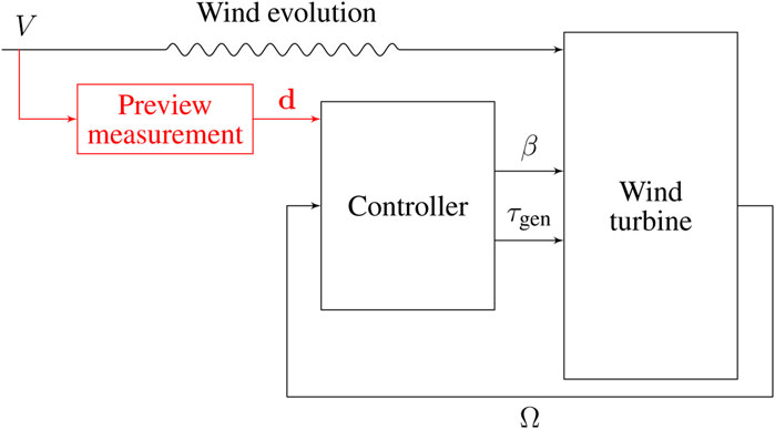
FIGURE 1. Block diagram of the wind turbine control system. Standard feedback components are shown in black, while additional components for feedforward control are shown in red.

1.2 Preview-enabled control

In addition to providing the energy required to turn the wind turbine rotor and generate power, the wind field is the main source of disturbances to the wind turbine control system. In particular, spatial and temporal variations in the wind speed cause the aerodynamic torque on the turbine rotor to fluctuate over time, in turn causing fluctuations in the rotational speed and requiring the feedback control system to constantly adjust the generator torque and blade pitch angle to maintain the rotor speed set point. Standard feedback-based architectures, such as the components shown in black in Figure 1, require that a change in the rotational speed Ω is measured before control action is taken to mitigate the disturbance. The feedback approach is very robust, but incurs delays because the effect of the disturbance must be experienced by the wind turbine before action is taken. This delay is amplified by the inertia of the turbine rotor and limited speed of blade pitch actuators.

The delays inherent to the feedback control system can be overcome by adding feedforward control action, which “preactuates” the blade pitch angle in anticipation of oncoming disturbances before they impact the turbine. To implement such feedforward control, a preview measurement of the oncoming disturbance must be taken. This is shown by the red elements in Figure 1. For wind turbine applications, lidar scanners have been shown to be capable of capturing the measurements of the wind field upstream of the turbine that are needed for preview-enabled control (Harris et al., 2005).

Various control architectures have been proposed and studied for preview-enabled control of wind turbines (Scholbrock et al., 2016). Of the methods investigated in the literature, model predictive control (MPC) has emerged as a popular approach (Lio et al., 2014), in part for its natural handling of future disturbances such as those provided by lidars. While MPC has been popular and shown promising results in simulation-based studies, physical experiments of preview-enabled MPC for wind turbines are scarce (Verwaal et al., 2015; Sinner et al., 2022). We are aware of two such studies. Verwaal et al. (2015) were the first to publish an experimental work demonstrating preview-enabled MPC of wind turbines, using a scaled model wind turbine. Their work was limited to a non-standard torque control in above-rated operation and low-frequency disturbances due to the hardware available. The study of Sinner et al. (2022) (the authors of the present work) instead used a fully-actuated scaled model wind turbine and more realistic disturbances, using a hot-wire anemometer in place of a lidar to provide preview disturbance measurements.

1.3 Contribution and scope

Experimental demonstrations of novel control approaches such as preview-enabled MPC are critical for translating promising simulation-based performance to industry adoption. Beyond proving a concept in reality, experiments also reveal important deficiencies and practical issues that may not appear in a computer simulation environment. An important practical issue for preview-enabled wind turbine control is the propagation time between the disturbance measurement location (upstream of the turbine), and the turbine location itself.

In this study, we consider this propagation time and investigate the sensitivity of control performance to accurate propagation time modeling with an experimental campaign on a scaled model wind turbine operating in a wind tunnel. We use MPC for the controller in our experiments, although we expect that the trends seen should broadly apply to any preview-enabled wind turbine control architecture. The rest of this paper proceeds as follows. In Section 2, we describe the propagation time in more detail and discuss other studies that have looked into propagation time modeling. We describe our experimental approach for investigating propagation time in Section 3 and provide numerical results in Section 4. We finish with further discussion of results in Section 5 and conclusions in Section 6.

2 Wind preview disturbance measurements and processing

In general, wind fields are complex, with spatial and temporal differences crossing a wide frequency spectrum. Variations in wind speed are the dominant disturbances to the wind turbine, and are the focus of this study. For real-time wind turbine control, we are most interested in distance scales on the order of the wind turbine rotor diameter, and temporal changes on the order of the time constant of the closed-loop wind turbine control system. These considerations have informed the design and operation of lidar scanners to extract useful information from the oncoming wind (Simley et al., 2014).

For the purpose of the discussion that this paper considers, the wind speed disturbance measurement location will be treated as a point location. In reality, continuous-wave lidar scanners sample a spread of locations in space, as shown in the left diagram of Figure 2. However, a weighting function is applied to amplify the measurements from the intended location, referred to as the focal distance, and lidar measurements are treated as though they are taken at a single discrete upstream location (pulsed lidars with multiple range gates notwithstanding). Simley et al. (2014) report that the optimal measurement location is approximately 1.1–1.5 rotor diameters (1.1D–1.5D) upstream of the wind turbine. Further, the lidar generally scans a pattern (or sweep) of points in the 2-dimensional plane at the measurement location, as shown in the right diagram of Figure 2, and averaged to generate a scalar wind speed measurement. As with spreading, we will proceed under the assumption that the averaging has already taken place and treat the lidar measurement as a scalar, rotor-effective wind speed (indicated in blue in Figure 2). For more details on processing raw lidar measurements, we refer readers to Simley et al. (2018) and the work of Simley generally.

FIGURE 2

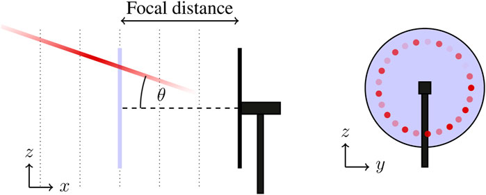
FIGURE 2. Aspects of the raw lidar sampling approach, including spreading along beam, line-of-sight limitations, and scan patterns shown in red, and their post-processed signal, the rotor-effective wind speed at the focal distance, shown in blue.

2.1 Disturbance propagation

The wind field undergoes two important dynamic changes between the upstream measurement location and the wind turbine locations: advection, referring to the transport of the air mass between the locations driven by the bulk fluid movement, and evolution, referring to the changes in wind field as it advects, driven by turbulence. The advection is the main concern of this paper; evolution has been investigated thoroughly by, e.g., Simley and Pao (2015) and informs the choice of filter described in Section 2.2. The flow advection speed is the key determinant of the delay that should be applied between the time when the upstream wind speed measurement is taken and the time that the measured wind field impacts the turbine and should be used by the wind turbine controller. We refer to this delay as the “propagation time.” Some authors have referred to the delay as the “arrival time.”

Most works, including our previous study (Sinner et al., 2022), assume that the wind propagates according to Taylor’s frozen turbulence hypothesis (Taylor, 1938). The frozen turbulence hypothesis postulates that larger turbulent structures (eddies) in the flow, such as those that are of a similar scale to the wind turbine rotor and are of concern for wind turbine control, travel downstream at the mean underlying wind speed. This makes computing the propagation time particularly straightforward: the propagation time is then simply the focal distance divided by the mean underlying wind speed, i.e.

$t_{\text{prop}}=\frac{d}{\bar{u}},(1)$

where t_prop is the propagation time; d is the distance between the measurement location and wind turbine (see Figure 2), and $\bar{u}$ is the underlying mean wind speed of the wind field V, assumed to be perpendicular to the turbine rotor (i.e., transverse and vertical components of the mean flow are assumed to be zero). Schlipf et al. (2010) studied the applicability of the frozen turbulence hypothesis for lidar-based wind turbine control applications on a utility-scale wind turbine, and demonstrated results that were consistent with the hypothesis.

Actuator disc theory describes the process by which momentum is extracted from the flow by a wind turbine and converted into kinetic energy spinning the wind turbine rotor (Burton et al., 2011, ch. 3). One of the major consequences from actuator disc theory is a slow-down of the bulk airflow as it passes through the wind turbine. This slow-down begins well upstream of the turbine, with the flow decelerating as it approaches the turbine. This deceleration region is referred to as the “induction zone” of the wind turbine. The presence of the induction zone has been confirmed in various experimental studies (e.g., Simley et al., 2016). The induction zone in front of the turbine suggests that the mean wind speed $\bar{u}$ in front of the turbine is a function of the upstream distance, meaning that the simple propagation time (1) from the frozen turbulence hypothesis is inaccurate.

Dunne et al. (2014) investigate a correction to the frozen turbulence model (1) to account for the induction zone based on actuator disc theory (Medici et al., 2011), and present experimental results to support their model. The corrected model, which still treats $\bar{u}$ as the free stream velocity outside of the induction zone, takes the form

$t_{\text{prop}}=\frac{d}{\bar{u}}M\left(d,a\right),(2)$

where M(d, a) depends on both the distance of the measurement point upstream of the turbine and the wind turbine’s axial induction factor a. M is expected to take values greater than 1. The axial induction factor describes the change in wind speed between a far upstream location and the wind turbine (Burton et al., 2011, ch. 3), and depends on the wind speed and the wind turbine’s rotational speed and blade pitch angle, which are dynamically changing during operation. This further complicates the matter of accurately estimating the propagation time.

2.2 Processing

In addition to advection, the wind field evolves between the measurement location and the turbine. High-frequency turbulence does not conform to the frozen turbulence hypothesis and should be removed from the wind speed measurement before it is used by the feedforward controller to prevent erroneous actuation (Simley et al., 2018). A low-pass filter is used to remove high-frequency turbulence. Filtering imparts a delay t_delay (known as the “group delay”) on the measurement such that the low-pass filtered output lags the input signal. This group delay should be removed from the propagation time when determining when the disturbance will arrive at the wind turbine.

For most filters, the group delay is frequency-dependent, meaning that the amount of delay imparted by the filter is not constant, creating a potentially difficult situation in determining the appropriate time to provide the filtered wind speed measurement to the controller. To avoid this issue we use a moving average filter, which has a frequency-independent group delay, in filtering upstream measurements.

The experimental apparatus that we use for our experiment, described further in Section 2.3, is digital. In subsequent discussion, we will therefore refer to time steps k, rather than times t. Time can be recovered as t = kT_s, where T_s = 0.01 s is the sampling time of the digital system (that is, a sampling rate of f_s = 100 Hz). Accordingly, we define $n_{\text{prop}}=\mathrm{r}\mathrm{o}\mathrm{u}\mathrm{n}\mathrm{d}\left(t_{\text{prop}}/T_s\right)$, where $\mathrm{r}\mathrm{o}\mathrm{u}\mathrm{n}\mathrm{d}\left(\cdot \right)$ rounds its argument to the nearest integer, and denote the filter group delay (in terms of time steps) by n_delay. The group delay of a constant magnitude, moving average filter with n_filt samples (where n_filt is an odd integer) is n_delay = (n_filt − 1)/2.

Finally, some preview-enabled controllers, including the model predictive controller (MPC) we use in our experiment, utilize knowledge of the wind speed measurement some time before the wind field impacts the turbine for planning purposes (prediction). We let n_control denote the number of time steps ahead that the controller requires the preview measurement. This is equivalent to the prediction horizon of the MPC. To align the filtered measurement with the assumed advection of the wind, the filtered measurement should be held in a buffer for n_buffer time steps, where

$n_{\text{buffer}}=n_{\text{prop}}-n_{\text{delay}}-n_{\text{control}}.(3)$

This relationship is also shown graphically in Figure 4.

2.3 Experimental testbed

In our experiment, we indirectly investigate the advection between the upstream measurement location and the wind turbine by comparing controller performance under a range of assumed propagation times. We run our experiments using a fully actuated, scaled model wind turbine (Figure 3A) operating in a wind tunnel testbed (Figure 3B) at the ForWind Center for Wind Energy Research in Oldenburg, Germany. The physical components of the testbed, described next, are identical to those used for our previous study (Sinner et al., 2022).

FIGURE 3

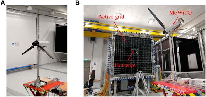
FIGURE 3. Wind tunnel experimental test bed at the ForWind Center for Wind Energy Research in Oldenburg, Germany. (A) The Model Wind Turbine Oldenburg (MoWiTO) used for the experiments. (B) MoWiTO in wind tunnel with active grid and hot-wire anemometer.

The Model Wind Turbine Oldenburg (MoWiTO 1.8), which is designed as an aerodynamically scaled version of the NREL 5 MW reference wind turbine (Jonkman et al., 2009), has a rotor diameter of 1.8 m and a rated operational speed (for this experiment) of 480 rpm. Preview measurements are taken using a tungsten hot-wire anemometer that is 1 mm long and 5 µm thick (in place of a lidar) placed 2.7 m, i.e., 1.5D, upstream of the turbine. The hot-wire anemometer is calibrated prior to each test session, and has an output signal standard deviation due to electrical noise of less than 0.3 m/s at the wind speeds tested. The blade pitch system encoder has a quantization error of 0.17° and the rotor shaft encoder has a quantization error of 4.17 rpm during run-time. However, after post-processing (which includes filtering), the rotor speed error is considered to be less than 1 rpm. For details on the MoWiTO, we refer the reader to Berger et al. (2018).

An active grid (Neuhaus et al., 2021) is used to generate complex inflows to the wind turbine. The controller, filter, and holding buffer are implemented in LabVIEW and deployed on National Instruments real-time controller hardware with a sampling rate of 100 Hz. The moving average filter uses n_filt = 35 samples. Figures 3B, 4 demonstrate the components of the testbed in photographic and schematic form, respectively. Given the 1.5D spacing between the hot-wire anemometer and the turbine, for above-rated wind turbine operation where a ≤ 0.33, Dunne et al. (2014) suggest that the value for M in the induction zone-corrected model (2) should be in the range 1.0–1.1 (see especially Figure 6 from Dunne et al. (2014)).

FIGURE 4

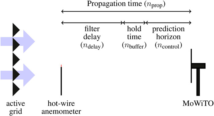
FIGURE 4. Diagram of the experimental testbed as well as the relationship between various components of the propagation time (represented by their number of time steps).

The MPC used for the experiments is designed to maintain the rated rotor speed in above-rated operation using blade pitch actuation. The model is a first-order linear response of the rotor speed to blade pitch and wind speed inputs, and the MPC objective function includes penalties on the rotor speed tracking error and its integral (state penalties) and on changes to the blade pitch angle (input penalty). Constraints include the blade pitch rate limit and absolute blade pitch angle limit. The MPC prediction horizon is set as n_control = 10 time steps. See Sinner et al. (2022) for full details on the controller development and implementation.

3 Experimental method

To determine the effect of the assumed propagation time on feedforward controller performance, we run repeated wind sequences through the wind tunnel while varying the length of the buffer n_buffer. The choice of filter size n_filt = 35 leads to a fixed group delay n_delay = 17. As the prediction horizon length is also fixed at n_control = 10, according to the relationship (3), altering n_buffer directly alters the assumed number of propagation time steps n_prop.

We run the experiment in two phases with distinct wind fields. In the first phase, a relatively simple gust wind input is provided to the turbine using the active grid (Figure 5A). The gust is repeated 10 times in sequence for each test value of n_buffer. Tested values of n_buffer are 5, 8, 11, 14, and 17, corresponding to values of n_prop of 32, 35, 38, 41, and 44. Thus, the range of values tested for the propagation time is 0.12 s, and the middle assumed propagation time (corresponding to n_prop) is 0.38 s. As the propagation time models (1) and (2) indicate, the mean wind speed in the tunnel $\bar{u}$ should affect the best choice for n_prop (with lower values of n_prop expected to perform better for higher wind speeds, and vice versa). We therefore repeat the ten-gust experiment at three different wind tunnel fan speeds (225 rpm, 239 rpm, and 253 rpm) corresponding to mean wind speeds of 6.3 m/s, 6.8 m/s, and 7.2 m/s, respectively, in the tunnel test section. As a control, we also run the sequence of 10 repeated gusts with the three fan speeds using an equivalent feedback-only (FB only) MPC (Sinner et al., 2022), which does not rely on preview wind disturbance measurements and therefore does not have a value for n_buffer or n_prop. For consistency, going forward, we will refer to preview-enabled configurations as “feedback/feedforward” (FB/FF) MPC. The testing matrix for the first phase is given in Table 1.

FIGURE 5

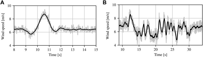
FIGURE 5. Input sequences used for experiment. The gray line shows the raw hot-wire anemometer measurement and the black line shows the output of the moving average filter (advanced by the group delay n_delay to align the signals for plotting purposes). Each sequence was repeated 10 times for each preview delay length. (A) Single instance of gust input sequence for phase 1, with a mean tunnel wind speed of 6.3 m/s. (B) Single instance of turbulence input sequence for phase 2.

TABLE 1

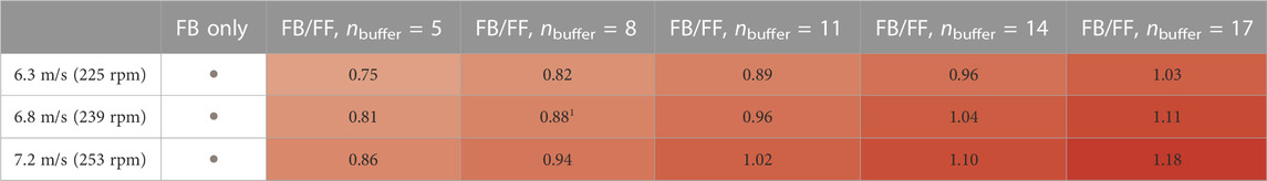
TABLE 1. Testing matrix for the first phase. Tunnel wind speeds (and corresponding fan speeds) are listed in the left-most column, while values for n_buffer are listed in the upper row. For each wind speed-n_d combination, a test set consisting of a repetition of ten gusts similar to that shown in Figure 5A is run. The gray dots denote the control case, which uses a feedback-only MPC that has no measurement of oncoming disturbances. The red cells denote the feedback/feedforward cases (which use preview measurements), where the number in the cell represents the equivalent M from the induction-zone corrected model (2) for the given wind speed-n_d combination and the shade of the cell represents the relative magnitude of M.

During the second phase, we run a more complex wind input sequence, representative of realistic turbulent inflow with a turbulence intensity of 18%. Again, the same wind input sequence is repeated ten times. A single instance of the ten-times repeated sequence is given in Figure 5B. For the second phase experiment, a single tunnel fan speed (263 rpm) is used, corresponding to a mean tunnel wind speed of 6.6 m/s for this input. Tested values of n_buffer are 7, 9, 11, 13, and 15, corresponding to values of n_prop of 34, 36, 38, 40, and 42. The control case (FB only MPC) is also run. The testing matrix for the second phase is given in Table 2.

TABLE 2

TABLE 2. Testing matrix for the second phase. The tunnel base wind speed (and corresponding fan speed) is shown in the left-most column, while values for n_buffer are listed in the upper row. For each wind speed-n_d combination, a test set consisting of a repetition of ten turbulent sequences similar to that shown in Figure 5B is run. As in Table 1, the shades and values in the cells represent the equivalent M for each wind speed and n_buffer combination.

4 Results

The controller’s primary objective is to regulate the rotor speed to the rated speed of 480 rpm using the blade pitch angle. Figures 6, 7 provide demonstrative time series responses from the phase 1 and phase 2 experiments, respectively. Note that the blade pitch angle (control input) for the FB/FF controller slightly leads that of the FB only case due to the wind speed disturbance preview, leading to improved rotor speed regulation.

FIGURE 6

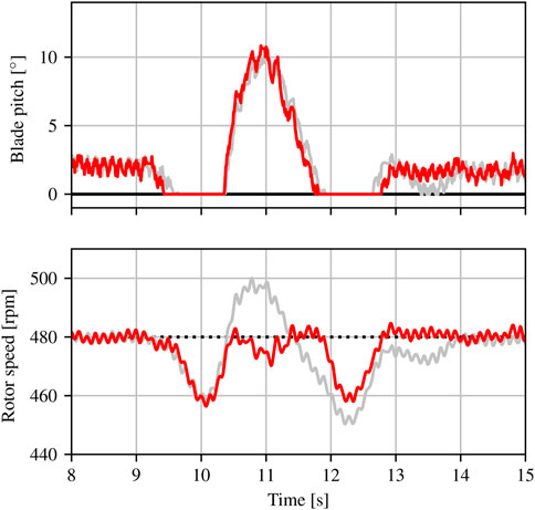
FIGURE 6. Responses of the FB only controller (gray) and FB/FF controller with n_buffer =11 (red) for a single gust at base wind speed 6.3 m/s from the phase 1 experiment. The upper plots show the blade pitch angle (control input) and the lower plots show the rotor speed (plant output).

FIGURE 7

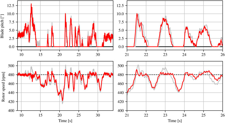
FIGURE 7. Responses of the FB only controller (gray) and FB/FF controller with n_buffer =11 (red) for a single turbulent sequence from the phase 2 experiment. The upper plots show the blade pitch angle (control input) and the lower plots show the rotor speed (plant output). The plots on the left show the response over the entire sequence, whereas the plots on the right show a subset of the response for detail.

We quantify performance in terms of features of the rotor speed response. For the phase 1 gust experiment, we look at the peak rotor speed deviations away from the rated speed as the clearest indicator of controller performance. For the phase 2 experiment, where there are multiple peaks and troughs over the turbulent wind sequence, the peak values do not convey useful information. Instead, we look at the root-mean-square (RMS) rotor speed error from the rated speed over the sequence to inform us of controller performance. It should be noted that because the turbulent flow is a transitional wind sequence containing both below-rated and above-rated operation, there are extended periods when the blade pitch controller is inactive and the torque controller takes over, which plays a significant role in the reported RMS errors. Nonetheless, the FB/FF controller should help to maintain above-rated operation and we still consider the RMS error a reasonable metric for the phase 2 experiment.

The peaks of the rotor speed response for each of the ten gusts for the phase 1 experiment are shown in Figure 8. The mean over the ten peaks is shown as a circle, and is provided numerically in Tables 3, 4 for clarity. Similarly, the RMS rotor speed errors for the phase 2 experiment are given in Figure 9, with means reported in Table 5. Along with the experimental results, we plot the (real-valued) choice of buffer size predicted by the frozen turbulence hypothesis, i.e., corresponding to M = 1.0 in the corrected model (2), as a vertical black line. For exposition, we allow this choice to take non-integer values.

FIGURE 8

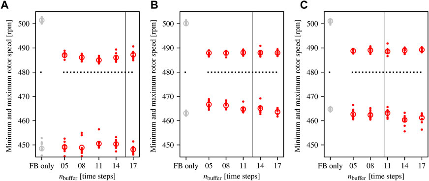
FIGURE 8. Peak rotor speed responses in the phase 1 experiment. The dotted line represents the rated rotor speed that the controller is targeting. Each point above (resp. below) the dotted line represents the maximum (resp. minimum) rotor speed during one of the ten gusts. The circular marker ◦ denotes the mean of the maximum or minimum over the ten gusts. The FB only control case is shown in gray, while FB/FF test cases are shown in red. The vertical black line indicates the buffer size suggested by the frozen turbulence hypothesis. (A) 6.3 m/s. (B) 6.8 m/s. (C) 7.2 m/s.

TABLE 3

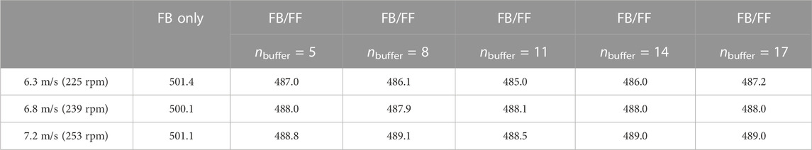
TABLE 3. Mean value of the maximum rotor speeds over the ten gusts during the phase 1 experiment, for each value of n_buffer (including the FB only configuration) and each tunnel wind speed.

TABLE 4

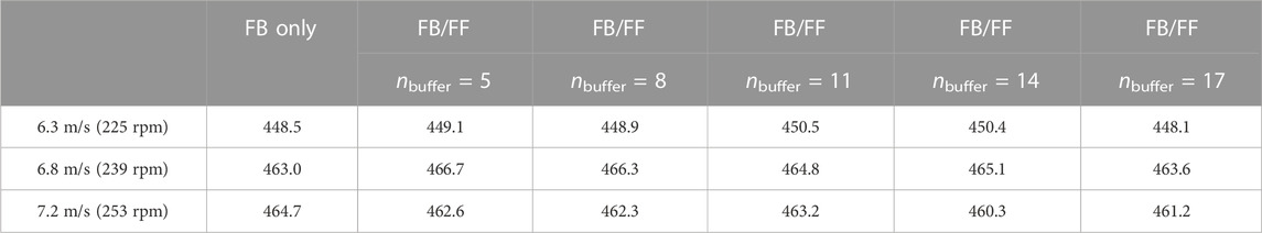
TABLE 4. Mean value of the minimum rotor speeds over the ten gusts during the phase 1 experiment, for each value of n_buffer (including the FB only configuration) and each tunnel wind speed.

FIGURE 9

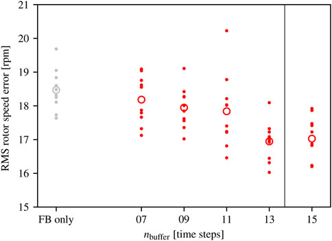
FIGURE 9. RMS rotor speed errors in the phase 2 experiment. Each point represents RMS rotor speed error during one of the ten gusts. The circular marker ◦ denotes the mean RMS error over the ten gusts. The FB only control case is shown in gray, while FB/FF test cases are shown in red. The vertical black line indicates the buffer size suggested by the frozen turbulence hypothesis.

TABLE 5

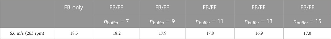
TABLE 5. Mean value of the RMS error over the ten repetitions of the turbulent sequence in the phase 2 experiment, for each value of n_buffer (including the FB only configuration).

5 Discussion

The results presented in Section 4 reinforce previous studies and experiments showing that the inclusion of feedforward control action can result in significant improvements in rotor speed regulation in above-rated operation. Overshoots in particular are dramatically reduced (Figure 8, as well as Figure 6). We now discuss the results of the test in more detail.

5.1 Qualitative analysis

Considering the phase 1 experiment (repeated gusts at various base wind speeds), several important trends are present besides the clear improvement in overspeed performance using preview-enabled control. First, the improvement in the minimum rotor speeds for FB/FF over FB only is less apparent than the improvement in maximum rotor speeds. This is again consistent with our previous findings (Sinner et al., 2022), and may partly be explained by the transition into below-rated operation during the lull before and after the gust, which cause the blade pitch angle to saturate at its low value of 0° and the rotor speed to drop. We therefore focus mostly on the maximum rotor speeds in the following.

Second, and perhaps most important, is an overall insensitivity to the assumed propagation delay. Across all three wind speeds tested, the FB/FF controller limits rotor overspeeds for all values of n_buffer tested. Considering the range of test values, this result, while somewhat surprising, is good news for preview-enabled wind turbine control, as it suggests that controllers may be robust to errors of 20% or more to the assumed propagation delay. In particular, this means that the buffer length may not need to be reset for small changes in the mean wind speed, making implementation easier.

Finally, although small, there does appear to be some sensitivity in the controller performance to the value of n_buffer for the FB/FF cases (Figure 8A). At a base wind speed of 6.3 m/s, a buffer length of n_buffer = 11 (corresponding to a number of propagation steps n_prop = 38 and propagation time t_prop = 0.38 s) appears to be best for limiting rotor overspeed. This is in fact slightly shorter than the 0.43 s that the frozen turbulence hypothesis (1) would suggest at 6.3 m/s and 2.7 m separation, i.e., suggesting a value M = 0.9 < 1 in the induction-zone corrected model (2). This result is surprising, as the correction applied should account for a slow-down (M > 1), rather than a speed-up (M < 1) in the flow (Dunne et al., 2014). Performance appears to degrade steadily, though not strongly, for buffer lengths above and below n_buffer = 11. For the higher wind speed cases (6.8 m/s and 7.2 m/s, Figures 8B, C, respectively), the only apparent differences with buffer length are in the minimum rotor speed values. As mentioned above, the minimum rotor speed responses are less clearly indicative of the feedforward control action, and we refrain from making analyses based on differences in the minimum rotor speeds alone.

We do not suggest that a value of M < 1 is physically representative of the true propagation time of the disturbance; instead, we consider the value seen as an indication that the best choice of buffer time for feedforward control of wind turbines is not simply that which best predicts the arrival of the gust. For instance, measurement and unmodeled actuation delays may mean it is best to provide the disturbance to the feedforward controller slightly in advance of the anticipated arrival time; and the best buffer length may be controller dependent and require testing various values to identify. It is also important to note that both the standard (1) and corrected (2) hypotheses assume that the large turbulent structures do not deform as they propagate downstream. While this may be true in the atmosphere, the presence of boundaries in the wind tunnel testbed and limitations in achievable flows with the active grid leads to some deformation of the flow. In particular, the gust profile (Figure 5A) may tilt somewhat as it propagates towards the turbine, with the higher wind speeds at the peak of the gust arriving more quickly than the lower wind speeds in the troughs. While the deformation appears to be minor over the tunnel test section between the hot-wire anemometer and MoWiTO (Neuhaus et al., 2021, esp. supplementary material), this may effectively shorten the best buffer length for the controller in the gust tests.

The phase 2 experiment (with repeated turbulent inflow, see Figure 5B) was run to provide the controller with a more challenging, variable inflow. This results in many transitions between below- and above-rated operation over the sequence (Figure 7). As mentioned in Section 4, the periods of operation below rated speed contribute significantly to the RMS rotor speed error values reported in Figure 9; Table 5, and the benefit of feedforward action in this case appears smaller. However, considering Figure 7, the FB/FF controller is still performing well in terms of reducing overshoots of the rated rotor speed. The FB/FF controller again shows some performance sensitivity to buffer length, with n_buffer = 13 appearing best. This corresponds to a propagation time of t_prop = 40 s, which at the 6.6 m/s base wind speed is in good agreement with the uncorrected frozen turbulence hypothesis (M = 1.0 in the corrected hypothesis (2)).

5.2 Statistical tests

The experiments conducted in this study were not designed to achieve a certain level of statistical significance. Nonetheless, it is informative to examine statistical significance through p-value testing to indicate whether there is indeed a change in performance with buffer length. For the sake of this discussion, we use a 95% confidence level to test the null hypotheses. We first test whether, at each wind speed for the phase 1 experiment, there is a difference in the median value of the maximum rotor speed across all buffer length cases (groups), including the FB only case. Given the small sample size, we use the Kruskal-Wallis H-test, with the null hypothesis that all groups come from populations with equal medians (Corder and Foreman, 2009, ch. 6). Similarly for the phase 2 experiment, we test whether there is a difference in the median RMS error across all groups. p-values for each wind speed are reported in the first line of Table 6. In all cases, we see p-values less than 0.001 and can reject the null hypothesis.

TABLE 6

TABLE 6. p-values for Kruskal-Wallis H-tests.

We next exclude the FB only group and rerun the H-tests to investigate whether there is a statistically significant difference across FB/FF controllers with different values of n_buffer. The p-values for these tests are given in the second line of Table 6. Consistent with the trends visually evident in Figures 8, 9, the p-values are sufficient to reject the null hypothesis of equal medians for the 6.3 m/s gust (from phase 1) and 6.6 m/s turbulence (phase 2). We fail to reject the null hypothesis for the 6.8 m/s and 7.2 m/s gusts.

The second row of Table 6 identifies significant differences in the median performance scores for the 6.3 m/s gust and the 6.6 m/s turbulence. To investigate these cases further, we test whether there is a statistically significant pairwise difference between the group with the best mean performance and the other groups for both cases. For the 6.3 m/s gust, the best performer is n_buffer = 11, while for the 6.6 m/s turbulence, the best performer is n_buffer = 13. We run a Mann-Whitney U-test, with the null hypothesis that the two groups are drawn from the same distribution (Corder and Foreman, 2009, ch. 4), for each pair; p-values are reported in Tables 7, 8. With multiple pairwise comparisons such as this, we increase the probability that one of the null hypotheses is incorrectly rejected (type 1 error). To counterbalance this effect, we make the (conservative) Bonferroni correction to our confidence level (Corder and Foreman, 2009), and require a new confidence level of 100–5/4 = 98.8% to reject the null hypothesis. The pairwise comparisons of n_buffer = 11 to n_buffer = 5 and n_buffer = 17 in the 6.3 m/s gust case and n_buffer = 13 to n_buffer = 7 and n_buffer = 9 succeed in rejecting the null hypothesis at this confidence level, indicating statistically significant differences between the distributions.

TABLE 7

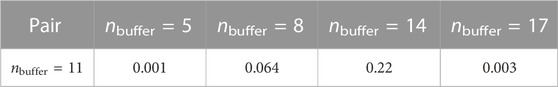
TABLE 7. p-values for pairwise Mann-Whitney U-tests for the 6.3 m/s gust maximum rotor speeds.

TABLE 8

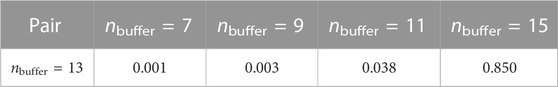
TABLE 8. p-values for pairwise Mann-Whitney U-tests for the 6.6 m/s turbulence RMS errors.

5.3 Simulated response

Finally, to support the evidence of insensitivity to the assumed propagation delay from the phase 1 and phase 2 wind tunnel tests, we ran computer simulations of the MoWiTO using the 10-gust input wind sequence at a mean wind speed of 7.2 m/s. This setup corresponds to the results presented in Figure 8C. We ran the simulations with all integer values of buffer size in the range [1, 30], and forced the “true” buffer size to n_buffer = 11 by providing a propagation time of t_prop = 0.38 s between the measured sequence and the sequence impacting the turbine. Random noise was added to the measured sequence to simulate electrical noise (which is then mostly removed by the moving average filter). No induction zone model is included (i.e., M = 1.0), and no wind evolution is modeled (i.e., the gust retains its shape between the measurement location and the wind turbine). Simulations were run in two configurations. In the first, the MoWiTO is modeled by a medium-fidelity nonlinear FAST model (Jonkman and Buhl Jr., 2005; Berger et al., 2018). In the second, the MoWiTO is modeled as a first-order linear system, which matches the model used by the controller perfectly. Minimum and maximum rotor speeds results analogous to those presented in Figure 8C are given in Figure 10.

FIGURE 10

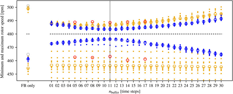
FIGURE 10. Simulated peak responses of the MoWiTO turbine for the 7.2 m/s phase 1 wind sequence. The brown data are produced using a medium-fidelity FAST model of the turbine whereas the blue data are produced using a linearized model that perfectly matches that used by the controller. The red (FB/FF) and gray (FB only) circles are the means from the corresponding wind tunnel test (see Figure 8C). The vertical black line indicates the “true” buffer sized used to run the simulation.

We note a few important differences between the simulated response and the wind tunnel experiments. First, the minimum rotor speeds for the FAST model are significantly lower. This is because the simulations do not include the MoWiTO’s torque controller, and instead the torque is kept at its maximum value throughout the simulations. The minimum speeds should therefore be ignored. The linear model does not have a torque model per se, and so does not suffer from this effect. Second, the maximum rotor speeds for the FB only case with the linear model, which had a mean value of 519 rpm, are not shown in the figure to allow us to focus on the trends in the FB/FF cases. We believe that the reason the peak overshoot is much higher for the linear model FB only case is that the linear model does not account for the increase in rotor speed sensitivity to blade pitch at higher blade pitch angles. This nonlinear effect tends to help prevent overshoot.

With these differences aside, the simulated responses strongly support the tunnel test results. In particular, the magnitudes of the maximum rotor speeds for the FAST model (plotted in brown) agree well with the tests (with slightly lower maximums in simulation than the wind tunnel experiment), and we again see that the maximum rotor speed is largely insensitive to the buffer size n_buffer. Increasing the buffer size to values about n_buffer = 20 (greater than a 20% error in the assumed propagation time), performance of the FB/FF controller starts to degrade noticeably, but does not approach the FB only controller’s performance until values around n_buffer = 30 (corresponding to a 50% error in the assumed propagation time). The response of the linear model (plotted in blue) is slightly less noisy because all modeling error is removed. Here, the trend is somewhat clearer due to reduced noise, with the best performance appearing at the expected value of n_buffer = 11 and a slow degradation in performance for lower and higher values of n_buffer. However, again, the overall performance sensitivity to the buffer size is low, reinforcing the results obtained in the wind tunnel experiments.

6 Conclusion and future prospects

In this paper, we investigated the sensitivity of a preview-enabled wind turbine blade pitch controller, utilizing upstream wind speed measurements, to the assumed propagation time for the wind speed disturbance. Experiments were conducted using a scaled model wind turbine operating in a wind tunnel testbed using a range of repeated test sequences and a range of assumed propagation delays. Our major conclusions from this study are as follows.

• The preview-enabled controller’s performance was rather insensitive to the assumed propagation delay, meaning that the controller has some degree of robustness. This is convenient for practical deployment of preview-enabled wind turbine controllers, as the assumed propagation delay may not need to be finely tuned to achieve the desired benefits of preview-enabled control.

• Although performance differences between the different assumed propagation times for the FB/FF case are relatively small, the preview-enabled controller performed best when the assumed propagation time was equal to or slightly less than the commonly-used frozen turbulence assumption, even though we would expect the induction zone in front of the turbine to slightly slow the flow. The reason may be that the delays due to pitch actuator dynamics, or model mismatch in the controller, mean that acting slightly early produced the best performance on sum. If so, the ideal propagation time may be turbine and controller dependent, and a testing period may always be needed to identify the best propagation delay.

Future prospects for assessing the role of assumed propagation time in preview-enabled wind turbine controllers’ performance include running similar experiments with different feedforward control architectures. This could help to determine whether the relative robustness of the FB/FF controller to the assumed propagation time is particularly strong in MPC or holds across a range of preview-enabled controllers. Moreover, similar experiments on an operational, utility-scale wind turbine using a lidar scanner instead of hot-wire anemometer would help to determine which, if any, of the effects seen in this study are particular to the wind tunnel experimental test bed.

Data availability statement

The raw data supporting the conclusion of this article will be made available by the authors, without undue reservation.

Author contributions

MS, VP, DS, MP, and LP contributed to the design of the experiments presented in this article. VP, MS, DS, and MP contributed to developing the controller and auxiliary code necessary for the experiment. VP and AL ran the wind tunnel experiments and collected data. The data was processed by VP, AL, and MS. DS ran supplementary simulations. Funding was provided by MK and LP. MS wrote the draft manuscript, and all authors read, provided comments on, and approved the submitted version. All authors contributed to the article and approved the submitted version.

Funding

This work was authored in part by the National Renewable Energy Laboratory, operated by Alliance for Sustainable Energy, LLC, for the U.S. Department of Energy (DOE) under Contract No. DE-AC36-08GO28308. Funding provided by the U.S. Department of Energy Office of Energy Efficiency and Renewable Energy Wind Energy Technologies Office. The authors gratefully acknowledge support from a Palmer Endowed Chair at the University of Colorado Boulder in the US and from the German State of Lower Saxony, which supported the wind tunnel campaign, active grid, and MoWiTO under the project “ventus efficiens.”

Acknowledgments

We thank Prof. Katya Arquilla for her insights on statistical testing.

Conflict of interest

The authors declare that the research was conducted in the absence of any commercial or financial relationships that could be construed as a potential conflict of interest.

Publisher’s note

All claims expressed in this article are solely those of the authors and do not necessarily represent those of their affiliated organizations, or those of the publisher, the editors and the reviewers. Any product that may be evaluated in this article, or claim that may be made by its manufacturer, is not guaranteed or endorsed by the publisher.

Author Disclaimer

The views expressed in the article do not necessarily represent the views of the DOE or the U.S. Government. The U.S. Government retains and the publisher, by accepting the article for publication, acknowledges that the U.S. Government retains a nonexclusive, paid-up, irrevocable, worldwide license to publish or reproduce the published form of this work, or allow others to do so, for U.S. Government purposes.

Footnotes

¹The combination n_buffer = 8, wind speed 6.8 m/s was run at a fan speed of 240 rpm rather than 239 rpm. This did not significantly change the tunnel wind speed.

References

Abbas, N. J., Zalkind, D. S., Pao, L., and Wright, A. (2022). A reference open-source controller for fixed and floating offshore wind turbines. Wind Energy Sci. 7, 53–73. doi:10.5194/wes-7-53-2022

CrossRef Full Text | Google Scholar

Berger, F., Kröger, L., Onnen, D., Petrović, V., and Kühn, M. (2018). Scaled wind turbine setup in a turbulent wind tunnel. J. Phys. Conf. Ser. (Deep Sea Offshore Wind R&D Conf.) 1104, 012026. doi:10.1088/1742-6596/1104/1/012026

CrossRef Full Text | Google Scholar

Burton, T., Jenkins, N., Sharpe, D., and Bossanyi, E. (2011). Wind energy handbook. New Jersey, United States: John Wiley & Sons, Ltd.

Google Scholar

Corder, G. W., and Foreman, D. I. (2009). Nonparametric statistics for non-statisticians. 1 edn. New Jersey, United States: John Wiley & Sons, Ltd. doi:10.1002/9781118165881

CrossRef Full Text | Google Scholar

Dunne, F., Pao, L., Schlipf, D., and Scholbrock, A. (2014). “Importance of lidar measurement timing accuracy for wind turbine control,” in Proc. American Control Conf., Portland, OR, June 4 - 6, 2014, 3716.

CrossRef Full Text | Google Scholar

Harris, M., Hand, M., and Wright, A. (2005). Lidar for turbine control. Tech. Rep. NREL/TP-500-39154. Golden, CO: NREL.

Google Scholar

Jonkman, J., and Buhl, M. (2005). FAST user’s guide. Tech. Rep. NREL/EL-500-38230. Golden, CO: NREL. doi:10.2172/15020796

CrossRef Full Text | Google Scholar

Jonkman, J., Butterfield, S., Musial, W., and Scott, G. (2009). Definition of a 5-MW reference wind turbine for offshore system development. Tech. Rep. NREL/TP-500-38060. Golden, CO: NREL.

Google Scholar

Lio, W. H., Rossiter, J. A., and Jones, B. L. (2014). “A review on applications of model predictive control to wind turbines,” in UKACC Int. Conf. Control, Loughborough, UK, 9-11 July 2014, 673–678.

Google Scholar

Medici, D., Ivanell, S., Dahlberg, J.-Å., and Alfredsson, P. H. (2011). The upstream flow of a wind turbine: Blockage effect. Wind Energy 14, 691–697. doi:10.1002/we.451

CrossRef Full Text | Google Scholar

Neuhaus, L., Berger, F., Peinke, J., and Hölling, M. (2021). Exploring the capabilities of active grids. Exp. Fluids 62, 130. doi:10.1007/s00348-021-03224-5

CrossRef Full Text | Google Scholar

Pao, L., and Johnson, K. (2011). Control of wind turbines. IEEE Control Syst. Mag. 2011, 44–62.

Google Scholar

Schlipf, D., Trabucchi, D., Bischoff, O., Hofsäß, M., Mann, J., Mikkelsen, T., et al. (2010). “Testing of frozen turbulence hypothesis for wind turbine applications with a scanning lidar system,” in Proc. Int. Symp. Advancement of boundary layer remote sensing (Paris, France: Larousse).

Google Scholar

Scholbrock, A., Fleming, P., Schlipf, D., Wright, A., Johnson, K., and Wang, N. (2016). “Lidar-enhanced wind turbine control: Past, present, and future,” in Proc. American Control Conf., Boston, MA, July 6-8, 2016, 1399–1406.

CrossRef Full Text | Google Scholar

Simley, E., Angelou, N., Mikkelsen, T., Sjöholm, M., Mann, J., and Pao, L. Y. (2016). Characterization of wind velocities in the upstream induction zone of a wind turbine using scanning continuous-wave lidars. J. Renew. Sustain. Energy 8, 013301. doi:10.1063/1.4940025

CrossRef Full Text | Google Scholar

Simley, E., Fürst, H., Haizmann, F., and Schlipf, D. (2018). Optimizing lidars for wind turbine control applications—Results from the IEA wind task 32 workshop. Remote Sens. 10, 863. doi:10.3390/rs10060863

CrossRef Full Text | Google Scholar

Simley, E., and Pao, L. (2015). “A longitudinal spatial coherence model for wind evolution based on large-eddy simulation,” in Proc. American Control Conf., Chicago, IL, July 1–3, 2015, 3708–3714.

CrossRef Full Text | Google Scholar

Simley, E., Pao, L. Y., Frehlich, R., Jonkman, B., and Kelley, N. (2014). Analysis of light detection and ranging wind speed measurements for wind turbine control. Wind Energy 17, 413–433. doi:10.1002/we.1584

CrossRef Full Text | Google Scholar

Sinner, M., Petrović, V., Langidis, A., Neuhaus, L., Hölling, M., Kühn, M., et al. (2022). Experimental testing of a preview-enabled model predictive controller for blade pitch control of wind turbines. IEEE Trans. Control Syst. Technol. 30, 583–597. doi:10.1109/tcst.2021.3070342

CrossRef Full Text | Google Scholar

Taylor, G. (1938). The spectrum of turbulence. Proc. R. Soc. Lond. 164.

CrossRef Full Text | Google Scholar

Verwaal, N., van der Veen, G., and van Wingerden, J.-W. (2015). Predictive control of an experimental wind turbine using preview wind speed measurements. Wind Energy 18, 385–398. doi:10.1002/we.1702

CrossRef Full Text | Google Scholar

Wiser, R., Bolinger, M., Hoen, B., Millstein, D., Rand, J., Barbose, G., et al. (2022). “Land-based wind market report,” in Tech. rep. (Berkeley, CA: U.S. DOE, LBNL).

Google Scholar