Computational Design of Sensitized Combustion Chemistry Experiments

In combustion chemistry experiments, reaction rates are often extracted from complex experiments using detailed models. To aid in this process, experiments are performed such that measurable quantities, such as species concentrations, flame speed, and ignition delay, are sensitive to reaction rates of interest. In this work, a systematic method for determining such sensitized experimental conditions is demonstrated. An open-source python script was created using the Cantera module to simulate thousands of 0D and hundreds of 1D combustion chemistry experiments in parallel across a broad, user-defined range of mixture conditions. The results of the simulation are post-processed to normalize and compare sensitivity values among reactions and across initial conditions for time-varying and steady-state simulations, in order to determine the “most useful” experimental conditions. This software can be utilized by researchers as a fast, user-friendly screening tool to determine the thermodynamic and mixture parameters for an experimental campaign. We demonstrate this software through two case studies comparing results of the 0D script against a shock tube experiment and results of the 1D script against a spherical flame experiment. In the shock tube case study we present mixture conditions compared to those used in the literature to study H + O₂ (+M)→HO₂(+M). In the flame case study, we present mixture conditions compared to those in the literature to study formyl radical (HCO) decomposition and oxidation reactions. The systematically determined experimental conditions identified in the present work are similar to the conditions chosen in the literature.

Introduction

In a typical combustion chemistry experiment attempting to measure a reaction rate, a set of conditions is chosen where a quantity that is sensitive to the target reaction rate can be measured. In shock tubes (Hanson and Davidson, 2014), some rapid compression machines (Mittal and Sung, 2007), and some flow reactor experiments (Dryer et al., 2014), this quantity is typically a species concentration as it varies in time. In stirred reactor (Burke et al., 2016) and some flow reactor configurations (Rasmussen et al., 2008; Guo et al., 2013) the species concentration at fixed residence time as it varies with temperature is measured. Occasionally, global parameters such as, ignition delay (Sung and Curran, 2014; Goldsborough et al., 2017) and flame speed (Santner et al., 2015) can be used to measure reaction rates. In each of these experiments, mixture conditions are chosen (within apparatus limits) such that measured quantities are sensitive to reaction rates of interest.

Sensitivity, S_i,j, can be computed by evaluating the normalized change in the ith dependent variable due to a normalized perturbation in the jth reaction rate (Eq. 1), or more specifically the pre-exponential factor A. Therefore, sensitivity analysis can determine the influence of each reaction rate on a measurable quantity. Sensitivity analysis is often used to improve mechanisms and influence experimental and theoretical efforts (Tomlin, 2013).

$S_{i,j}=\frac{\Delta y_i/y_i}{\Delta k_j/k_j}=\left(k/y\right)\left(dy/dk\right)=\frac{d\left(\ln y\right)}{d\left(\ln k\right)}(1)$

When performing an experiment with the goal of improving chemistry models, it is vital to choose mixture conditions where the measurement is sensitive to particular elementary reaction rates, while minimizing sensitivity to confounding reaction rates and other uncertain independent variables (reaction initiation, thermodynamic conditions, boundary conditions, etc.) However, experimental conditions are often chosen through intuition, expert opinion, prior results, convenience, and trial-and-error sensitivity analyses. Of course, experimental conditions are also constrained by the physical apparatus as well. Although this method has produced valuable data and predictive chemistry models, there is an opportunity for improvement.

In this work, we present two computational tools to aid in the choice of experiment conditions. These tools use sensitivity analysis to determine the experimental conditions that yield the most useful information about reaction rates. Two case studies were performed to compare experimental conditions to those identified in Choudhary et al. (2019) and Santner et al. (2015). These case studies were used in order to explain, validate, and improve our method. In Choudhary et al. (2019), OH concentration was measured in a shock tube for H₂/O₂/inert mixtures at 1,450–2,000 K in order to measure the reaction rate of H + O₂ (+M) → HO₂ (+M), where the third-body collider is argon, nitrogen, and carbon dioxide. In Santner et al. (2015), laminar burning rates of 1,3,5-trioxane/O₂/N₂ mixtures were measured in a spherical, heated, high pressure, constant volume chamber in order to measure the flame properties of formaldehyde (CH₂O) and formyl radical (HCO).

Methods

Code Overview: Commonalities of 0-D and 1-D Code

To operate the software, the user defines a range of parameters to simulate, the code creates mixtures based on user input, calculates sensitivity over that range of parameters, and the results are post-processed, organized, and plotted.

The thermodynamic state is defined from the user-defined pressure and temperature ranges. There are several methods to define the chemical composition of the mixture. Each mixture contains three components–a fuel, oxidizer, and diluent. To create more complex mixtures, each of these components can contain a fixed composition of multiple species. For example, the “fuel” can be defined as a 50/50 blend of H₂ and CO in order to simulate syngas. From these three components, a mixture can be defined using two of the following: the equivalence ratio, fuel/diluent ratio, oxidizer/diluent ratio, fuel mole fraction, oxidizer mole fraction, diluent mole fraction (see Supplementary Appendix SA for code input keywords). The user inputs a range of values for the two parameters that will be used to define the mixture. Mixture composition and thermodynamic parameters can be varied linearly or logarithmically between the given endpoints.

Each initial condition, defined by the mixture composition and thermodynamic state, is stored in a dictionary along with the sensitivities calculated by Cantera (Goodwin et al., 2009). Each simulation is independent, so they are performed in parallel to improve the computational speed.

After all cases have been simulated the results are post-processed. Most post-processing tasks are defined in detail in sections “Zero-Dimensional Simulations” and “One-Dimensional Simulations”, except for the treatment of duplicate reactions, which is common to both 0-D and 1-D simulations. Oftentimes, duplicate reactions are utilized in chemical mechanisms to simulate non-Arrhenius behavior. These reactions have individual sensitivities but are a part of a single reaction and are therefore summed in the software to find the actual sensitivity of the reaction.

Zero-Dimensional Simulations

Software was created in python to simulate a 0D constant pressure reactor and calculate sensitivity in Cantera (Goodwin et al., 2009) for a range of temperature, pressure, and mixture composition. After all cases have been simulated the results are run through a ranking process to determine which conditions allow for sensitive experiments. Simulations are rejected if the temperature rise is greater than 100 K (although this value can be adjusted by the user), signaling excessive heat release for a shock tube or flow reactor experiment. In an experiment, useful reaction data can only be quantified if the species of interest concentration is above detection limits. Therefore, sensitivities are set equal to zero whenever the concentration of the measurable species falls below a user-defined threshold. After these two filters, time-dependent sensitivities are then saved for post-processing and detailed analysis of particular conditions in a graphical user interface (GUI).

A major open question in this work is the method to determine which condition yields the most useful measurements. We present two techniques to quantify the information content of a simulation: S_max,i(t) and IS_i,j.

Our simplest quantifier is the time-dependent maximum sensitivity, S_max,i(t). This parameter is the reaction that species i is most sensitive to at time t. While easy to determine, S_max,i(t) does not incorporate the time-varying nature of experiments–it treats a 0D experiment as if it only utilizes measurements at one point in time. Additionally, it does not quantify the degree to which one reaction is more sensitive than others–it would provide the same result if the measured quantity is nearly as sensitive to the 2nd most sensitive reaction as to the 1st, or if one reaction dominates.

To provide a more quantitative measure, the integrated strength, IS_i,j, is defined as the integrated sensitivity of species i to reaction j over the entire time domain (Eq. 2). Inside of the integral of Eq. 2, the sensitivity is multiplied by a gate function, II(X_i), (Eq. 3), to indicate that experiments do not provide useful data when the species of interest is undetectable. Assuming experimental measurements are evenly spaced in time throughout the test period, IS_i,j determines the influence of reaction j on species i during a time-dependent experiment. In this paper, we use t_start= 0 s, however it could be delayed due to experiment considerations, such as the time shifting technique common in flow reactors (Rasmussen et al., 2008; Guo et al., 2013).

$I{S}_{i,j}={\displaystyle {\int }_{t_{start}}^{t_{end}}{S}_{i,j}\Pi \left(X_i\right)\text{d}t}(2)$

$\Pi \left(X_i\right)=\{\begin{array}{cc}1& \text{if }{X}_i\ge \text{detection}\text{limit}\\ 0& \text{if }{X}_i<\text{detection}\text{limit}\end{array}(3)$

IS_i,j quantifies the sensitivity over the entire time domain in order to compare and rank sensitivities within one simulation. However, it cannot be used to easily compare among simulations at varied thermodynamic conditions. In order to achieve this, and to indicate if a certain reaction dominates over others, the normalized integrated strength, ${\widehat{IS}}_{i,j}$ (Eq. 4), is defined as the integrated strength normalized by the average of the absolute value of integrated strength of the top five reactions (Eq. 5). It should be noted that the matrix that contains all sensitivities for each reaction (Eq. 5) is sorted by absolute value. Through this definition, ${\widehat{IS}}_{i,j}$ provides a value that is $\mathcal{O}\left(1\right)$, indicating the sensitivity of species i to reaction j integrated over the entire time domain, relative to other reactions. Although sensitivities are already normalized within Cantera, this normalization is necessary in order to compare sensitivities among different reactions, and at different conditions. This solves two problems. First, this normalization compares a sensitivity to others for the same simulation, indicating whether observables are significantly more sensitive to a particular reaction than to other reactions, as an experimentalist desires a condition where an observable is significantly more sensitive to one or two reactions than to all others. Second, it allows easy comparison among different simulation conditions. Without this additional normalization, effects that affect all sensitivities (such as increased temperature) would dominate over the desired metric–sensitivity of an observable to a reaction, relative to others at the same condition.

${\widehat{IS}}_{i,j}=\frac{I{S}_{i,j}}{{\overline{IS}}_{ i}}(4)$

${\overline{IS}}_{ i}=\frac{1}{5}{\displaystyle \sum }_{j=1}^5\left|I{S}_{i,j}\right|(5)$

In addition to the parameters described above, the 0-D software is also integrated with a GUI which allows the user to interact with a single simulation condition. With such a large dataset containing time-dependent predictions of multiple species concentrations for a broad range of initial conditions, the summary figures described above may motivate a closer look at individual conditions. The GUI displays the time-dependent sensitivity to the requested species for the five most sensitive reactions, and the concentrations of user-defined species. The GUI provides the user more detailed time-resolved information about specific species at a specified test condition.

One-Dimensional Simulations

Software was created in python to simulate a 1D adiabatic laminar flame, calculating flame speed and sensitivity in Cantera (Goodwin et al., 2009) over a range of user-defined thermodynamic conditions and mixture composition. Results are then saved for post-processing, and detailed analysis of the most sensitive reactions are written to. csv files.

The sensitivity of the flame speed to a reaction rate has little value unless it is compared to the sensitivity of other reactions. To provide this comparison, the normalized sensitivity, ${\widehat{S}}_j$ (Eq. 6), is defined as the sensitivity of the laminar flame speed to reaction j divided by the average sensitivity of the n most sensitive reactions (Eq. 7). Note that this normalization method is analogous to the method used in Zero-Dimensional Simulations (Eqs. 4, 5). We use n = 7 in this work, but this parameter is user-defined. The normalized sensitivity is a dimensionless number that indicates the reaction’s importance to the flame relative to other reactions. A value of ${\widehat{S}}_j$ significantly greater than 1 indicates that the flame speed is much more sensitive to reaction j than to other reactions.

${\widehat{S}}_j=\frac{S_j}{\overline{S}}(6)$

$\overline{S}=\frac{1}{n}{\displaystyle \sum }_{j=1}^n\left|S_j\right|(7)$

To expand on the method of normalized sensitivity, the code also calculates the average normalized sensitivity to reaction j, ${\overline{\widehat{S}}}_j$, across all cases (Eq. 8). This parameter indicates the sensitivity to a particular reaction across a broad range of conditions, showing the user which reactions should be investigated further. The results of this calculation are stored in a csv file to be viewed by the user. The code will also create a second csv of the n rxns with the highest average normalized sensitivity $\left({\overline{\widehat{S}}}_j\right)$, and creates figures of the top n rxns for the user to further analyze each reaction.

${\overline{\widehat{S}}}_j=\frac{{{\displaystyle \sum }}_{n=1}^n{\left|{\widehat{S}}_j\right|}_n}{n_{cases}}(8)$

Results and Discussion

Stanford Case Study

In order to measure H + O₂ (+N₂)→HO₂(+N₂), Choudhary et al. (2019). performed 9 experiments with 0.1% H₂/2%O₂/N₂ with temperatures from 1552–1908 K, and pressures from 9.35 to 21.68 atm. These conditions were chosen to improve the sensitivity of OH concentration to the target reaction rate [see Figure 7 in (Choudhary et al., 2019)]. The present software is applied over a broader range of conditions, as shown in Table 1. Over these conditions, 5,930 simulations were performed with a 1 ms residence time, which took 42 min and saved 280 kB of data. Simulations use the FFCM-1 model (Smith et al., 2016) with 292 reactions and 38 species for consistency with Choudhary et al.

TABLE 1

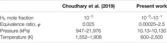
TABLE 1. Mixture conditions. The balance gas is nitrogen.

As a first step towards validation, Figure 1 shows a screenshot of the GUI reproducing Figure 8 (top) and 9 (top) from (Choudhary et al., 2019). The GUI loads the results of a large dataset, and the drop-down menus allow the user to choose the mixture condition (T, P, φ, X_fuel). The user chooses the species of interest (OH in this case) and the time of interest. The figure on the left plots the sensitivities of the five reactions with the largest sensitivity at the user-defined time of interest (indicated by the vertical line). The figure on the right plots the species-time evolution for the species selected from drop-down menus. This GUI allows the user to easily interrogate mixture conditions and obtain detailed time-domain results.

FIGURE 1

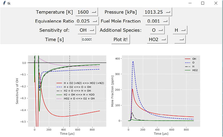
FIGURE 1. GUI screenshot.

Figure 2 demonstrates the reactions that are most important at each condition as quantified by S_max,i(750 μs). There appears to be a broad range of conditions where the target reaction (reaction 15) is most sensitive. However, the other reactions in the H₂–O₂ subset between reactions 1 and 27 appear to be sensitive over many conditions. Notably, reaction 270, H + O + M↔OH*+M, becomes most sensitive at extremely high temperatures and pressures.

FIGURE 2

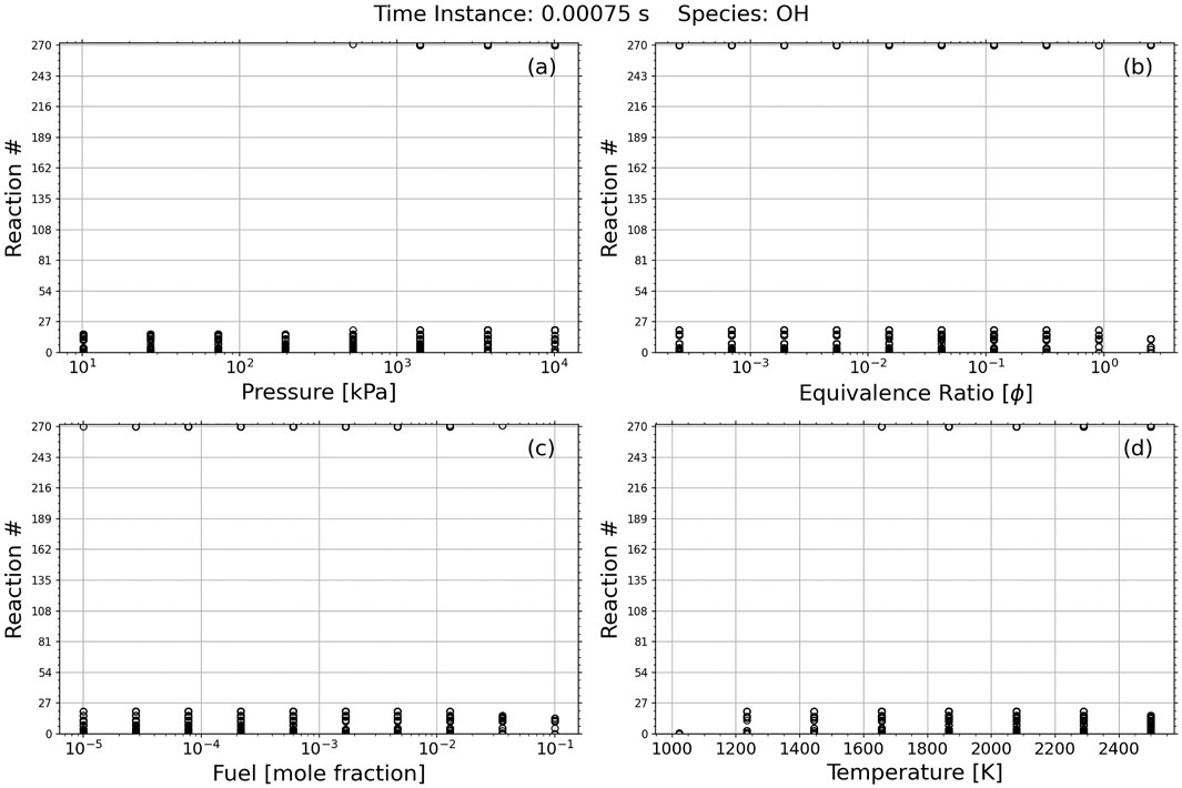
FIGURE 2. Most Sensitive reactions of OH at 750 μs.

Although Figure 2 indicates the conditions where the target reaction is most sensitive, it does not indicate the degree of sensitivity, or compare its sensitivity to that of other reactions. To accomplish this, Figure 3 demonstrates broad trends in the dependence of ${\widehat{IS}}_{OH, H+O_2\left(+N_2\right)\leftrightarrow H{O}_2\left(+N_2\right)}$ on temperature, pressure, equivalence ratio, and fuel mole fraction. Our method agrees with Choudhary et al. (2019) that OH measurements are most sensitive to the reaction of interest at the conditions in Table 1, which are indicated in Figure 3 by the blue dashed regions. Hydroxyl is expected to have a negative sensitivity to the reaction of interest, which is typically considered a chain terminating reaction. However, Figure 3D shows that OH has a positive sensitivity to HO₂ formation at high temperature, indicating an alternate pathway for OH formation through HO₂.

FIGURE 3

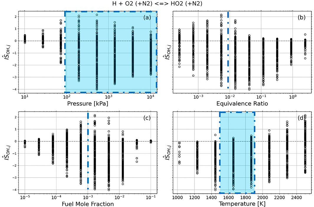
FIGURE 3. Trends in normalized integrated strength for the reaction of interest. The blue dashed lines and regions represent conditions of Choudhary et al. (2019).

With 5,930 overlapping simulation points displayed in Figure 3, it is difficult to determine the most sensitive conditions. To aid in this, the interdependence of mixture properties and sensitivity is shown in Figure 4. Each point represents a condition where OH mole fraction is most sensitive to the target reaction at 750 μs Several trends are apparent. Figure 4A shows that at nearly any T, P combination if T > 1200 K, there exists a mixture composition such that OH is most sensitive to the target reaction. Figures 4D,E indicate a broadening of useful mixture compositions as the pressure rises. Figures 4B,C similarly indicate a broader range of mixture composition as a temperature decreases from 2,500 to 1,200 K, until there are no conditions below 1,200 K where OH is most sensitive to H + O₂ (+N₂)→HO₂(+N₂). Finally, Figure 4F shows a correlation between equivalence ratio and fuel content. At high fuel content and low equivalence ratio, the mixtures are impossible (X_O2 > 1). At low fuel content and high equivalence ratio, reactivity is too low to produce OH concentrations above the assumed 1 ppm detection limit.

FIGURE 4

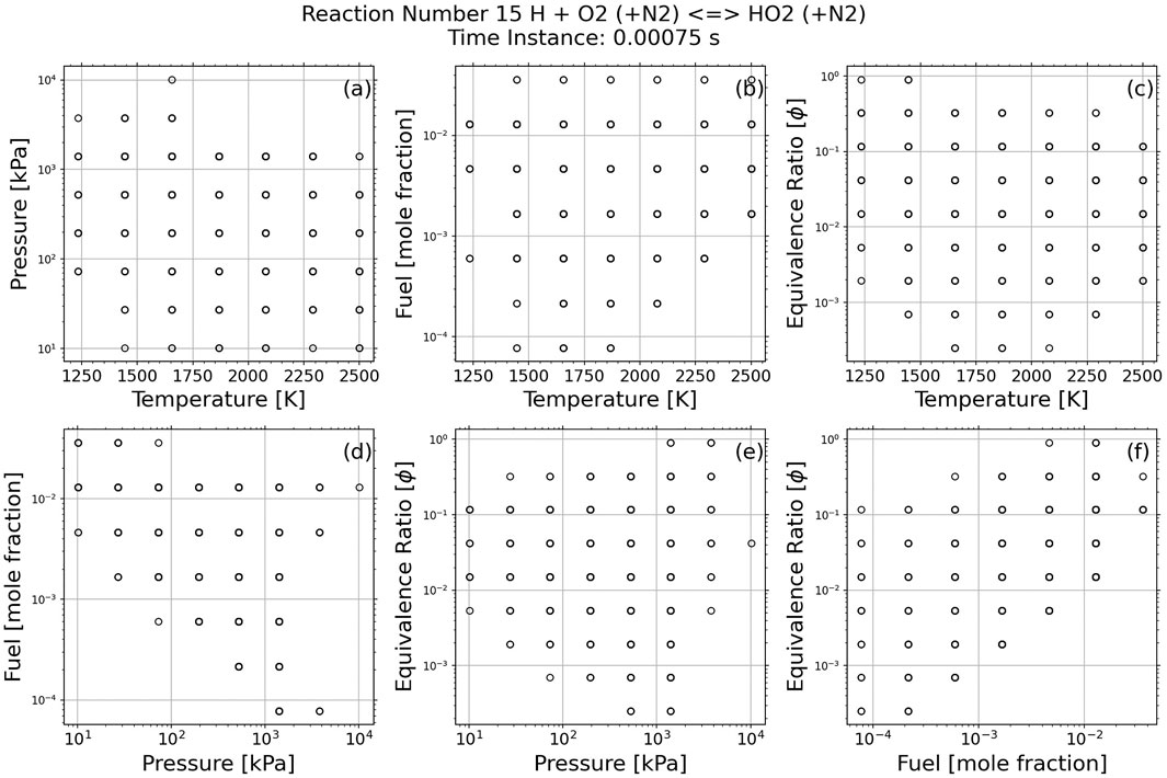
FIGURE 4. Conditions where reaction 15 is most sensitive for species OH.

Using the GUI, it is simple to investigate these trends. For example, at low pressure and low fuel mole fraction, OH is not sensitive to the reaction of interest, as shown in Figure 4D. At these low pressures, overall reactivity is decreased such that within the selected time window OH is sensitive to its fast formation reactions, such as H₂+O↔H + OH, rather than its slower destruction mechanism. Similarly, the dependence on temperature can be simply explained. At low temperature, particularly for low fuel content, reactivity is too low to produce detectable OH. At higher temperature, quasi-equilibrium is quickly reached such that OH is sensitive to dissociation and recombination reactions, although sensitivity values are low.

Santner et al. Case Study

In order to investigate reactions of formyl radical (HCO), Santner et al. (2015) measured the flame speed of trioxane/O₂/N₂ mixtures at 22 conditions as shown in Table 2. These conditions were chosen to improve the sensitivity of the flame speed to HCO + O₂↔CO + HO₂ and HCO + M↔H + CO + M (see Figures 2 and 4 in Santner et al., 2015). The present software was applied over a broader range of conditions, as seen in Table 2. Over these conditions, 288 simulations were performed with 242 cases converging taking a total of 22 min and 1,851 KB of data. Simulations use the Li et al. model (Li et al., 2007) modified to include trioxane reactions and species as in Santner et al. (2015).

TABLE 2

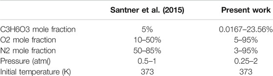
TABLE 2. Mixture Conditions. The balance gas is nitrogen.

As a first step of validation, Figure 5; Table 3 show the reactions that were most sensitive in each case. Over the range of conditions, reaction 29 (CO + OH↔CO₂+H) was the most sensitive in 968 cases. This is expected, as this reaction provides the majority of the heat release in the flame. Reaction 1 (H + O₂ ↔ O+ OH) shows maximum sensitivity in 254 cases, which is expected due to the strong chain-branching nature of this reaction. Reaction 46 (CH₂O+ HO₂ ↔ H₂O₂ + HCO) shows maximum sensitivity in 47 cases, and Reaction 13 [H + O₂ (+M) ↔ HO₂ (+M)] shows maximum sensitivity in 10, however from Figure 5 we can see that these cases have very low fuel mole fraction, where the flame speed would be so slow that it would be difficult to measure accurately. The reactions of interest, Reaction 30 (HCO + M ↔CO + H + M) and Reaction 31 (HCO + O₂ ↔CO + HO₂), were the most sensitive reaction for only 2 and one condition, respectively. Although these reactions are not the most sensitive, their rates have higher uncertainty than reactions 29 and 1, such that experiments should provide useful information.

FIGURE 5

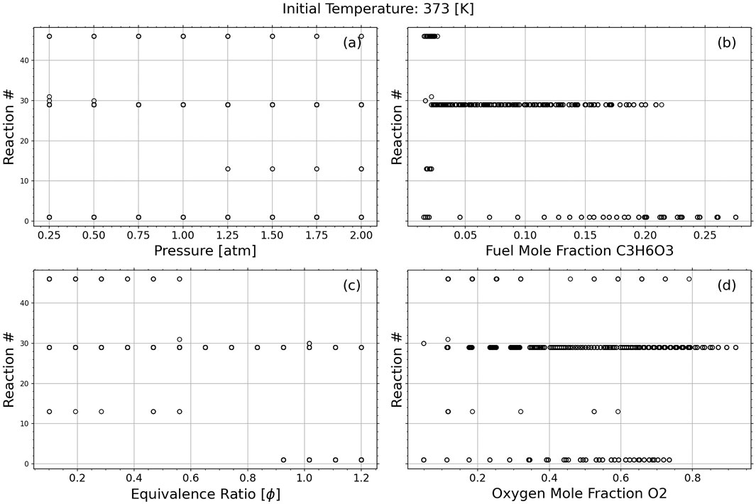
FIGURE 5. Most sensitive reactions per parameter.

TABLE 3

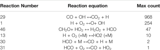
TABLE 3. Reactions that appear in Figure 5, including the number of conditions where the flame speed is most sensitive to each reaction.

In Figures 6, 7 we focus on each reaction of interest. The normalized sensitivity, as expressed in Eq. 5, shows how strong each reaction is compared against the top seven most sensitive reactions. In these figures we look at the effects of pressure, fuel mole fraction, oxygen mole fraction, and flame speed on the normalized reaction strength.

FIGURE 6

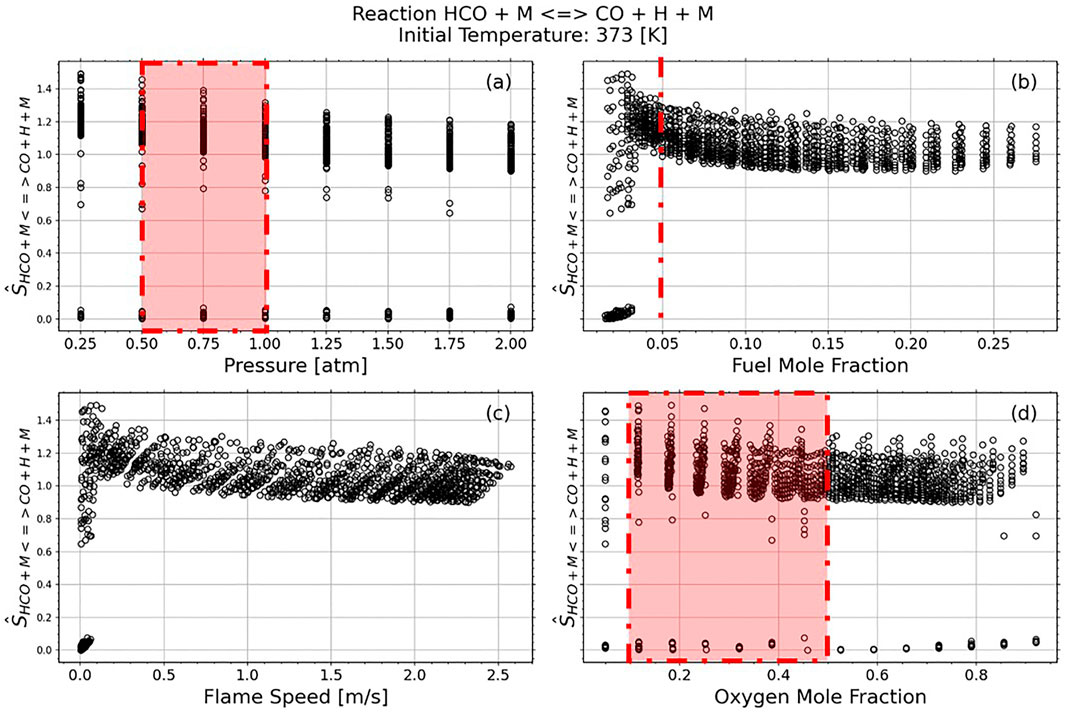
FIGURE 6. Reaction 30 HCO + M↔CO + H + M Normalized Sensitivity Strength against the top seven reactions per case. The red dashed lines indicate experimental conditions from Santner et al. (2015).

FIGURE 7

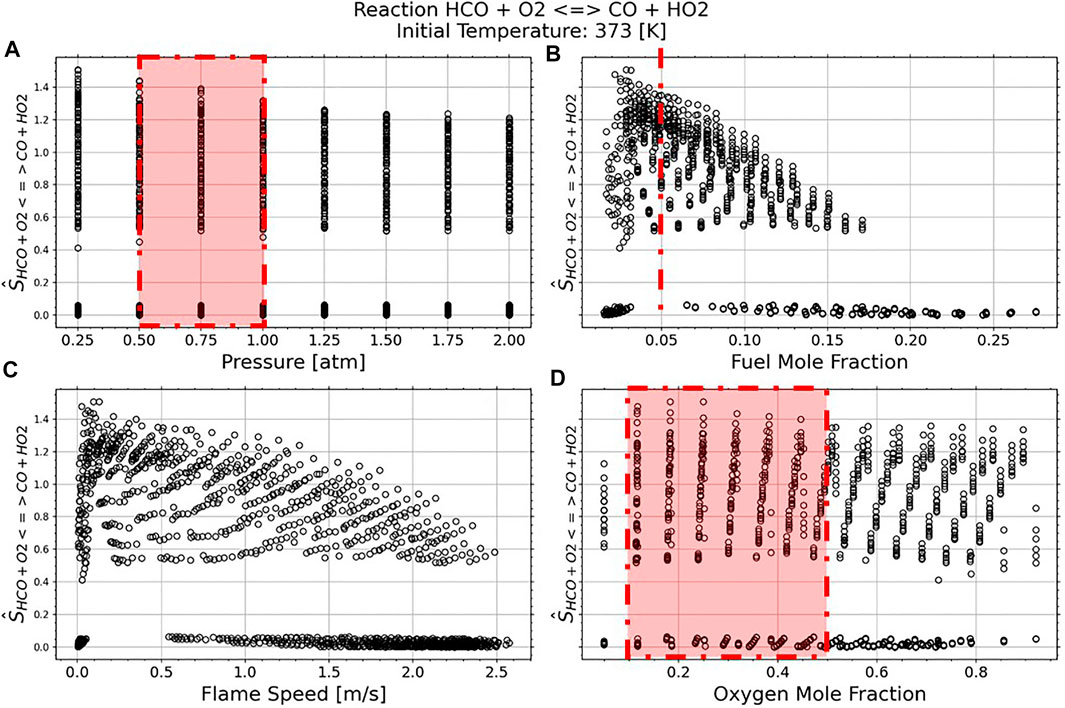
FIGURE 7. Reaction 31 HCO + O2↔CO + HO2 Normalized Sensitivity Strength against the top seven reactions per case. The red dashed lines indicate experimental conditions from Santner et al. (2015).

Figures 6B, 7B show that the normalized reaction sensitivity is near, or greater than, 1 for most conditions with fuel mole fractions between 2.5 and 5%, with maximum sensitivity occurring with a fuel mole fraction of 2.5%. This indicates that the flame is more sensitive to the target reaction than it is to the average of the top 7 most sensitive reactions. However, Figures 6C, 7C demonstrate that this maximally sensitized condition occurs with a flame speed of 0.1 m/s, which cannot be measured accurately in an expanding spherical flame due to radiation (Santner et al., 2014) and buoyancy (Qiao et al., 2007) effects. As indicated by the red regions in Figure 6, this result confirms the choices in Santner et al. (2015)—a 5% fuel mole fraction creates a mixture where the flame speed is sensitized to the target reaction rate, while producing fast enough flames to be accurately measured. Figures 6A, 7A demonstrate a slight increase in normalized sensitivity as pressure decreases, however low-pressure experiments are difficult due to the high critical ignition radius. For most cases, the oxygen mole fraction does not contribute to a change in normalized sensitivity strength.

The top 7 average normalized sensitivities, ${\overline{\widehat{S}}}_j$, are shown in Table 4 and calculated according to Eq. 8. This represents all cases performed in the simulation, where conditions are described in Table 3. From Table 4 we can see that reaction 29 is almost twice as sensitive as the next reaction, reaction 1. Flame speed is typically most sensitive to these two reactions, especially for small hydrocarbon fuels. They have been thoroughly studied and quantified. The target reactions in this study, reactions 30 and 31, are the 3rd and 4th most sensitive averaged over all cases. The next three most sensitive reactions have significantly lower average normalized sensitivity. Detailed figures for these reactions 17, 15, and 13, (Supplementary Appendix SB), show that the flame speed is significantly less sensitive to these reactions at the conditions where the flame speed is sensitive to reactions 30 and 31 (Figures 6C, 7C). Reactions 13, 15 and 17 are most sensitive for extremely low fuel mole fractions, particularly at higher pressures, where the target reactions (30 and 31) are less sensitive and an experiment is difficult to perform regardless. Thus, the experiments in (Santner et al., 2015) are performed at appropriate conditions where the flame speed is sensitized to the target reactions, within the constraints of the experimental apparatus, and assuming the chemistry model is accurate.

TABLE 4

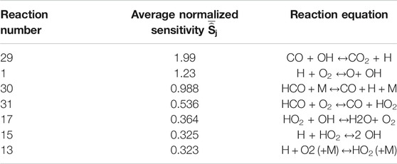
TABLE 4. Top seven reactions average normalize sensitivity.

Conclusion

A 0-D and 1-D software is presented that can streamline and formalize the process for determining experimental conditions. The 0D software evaluates the simulation results by integrating the sensitivity over time to provide a sensitivity strength over the span the experiment time. Sensitivities are normalized against the top n most sensitive reactions in order to compare the relative impact of a reaction on a measurable quantity across a range of initial conditions. Finally, these normalized sensitivities can be averaged over a broad range of thermodynamic and mixture conditions in order to identify wider trends.

Using these techniques, the results of the simulations are compared against the conditions chosen in Choudhary et al. (2019) and Santner et al. (2015), respectively, yielding similar results. In other words, the present, rigorous code would have chosen similar experimental conditions as (Santner et al., 2015; Choudhary et al., 2019) Finally, insight into the reaction mechanism is provided through the trends observed in summary plots. Included with the 0-D simulation is a GUI with the ability to interrogate individual simulations. Along with the 1-D simulation are csv files providing information on top n reactions, reactions that showed maximum sensitivity, and a list of all reactions involved with their average normalized sensitivity.

The present version of the software, version 1.0 is open-source and freely available at https://github.com/CSULA-Combustion-Lab/design-of-experiments

In the future, this software can be expanded beyond reaction rate sensitivity to include sensitivity to transport and thermodynamic parameters, which have been shown to be important in model predictions (Langer et al., 2021). Additionally, the optimization potential (product of sensitivity and uncertainty) (Cai and Pitsch, 2014; Langer et al., 2021) can be incorporated into this software.

Data Availability Statement

The datasets presented in this study can be found in online repositories. The names of the repository/repositories and accession number(s) can be found below: https://github.com/CSULA-Combustion-Lab/design-of-experiments

Author Contributions

JS is the PI of this project, contributing significantly to the code and text of the paper. PR and DL wrote an early version of the software with JS. This first draft of the software only included 0D simulations. PR focused on the simulations, and DL focused on the GUI. CI significantly improved on PR and DL’s original code. CI parallelized the software, reorganized and simplified it, and added the 1D simulations. CI also created the figures and the majority of the text in the manuscript.

Conflict of Interest

The authors declare that the research was conducted in the absence of any commercial or financial relationships that could be construed as a potential conflict of interest.

Acknowledgments

CI is the recipient of a CREST-CEaS fellowship, for which we are grateful. This work has been supported by an NSF HRD-1547723 Grant and the SoCalGas RD&D program.

Supplementary Material

The Supplementary Material for this article can be found online at: https://www.frontiersin.org/articles/10.3389/fmech.2021.705586/full#supplementary-material

References

Burke, U., Metcalfe, W. K., Burke, S. M., Heufer, K. A., Dagaut, P., and Curran, H. J. (2016). A Detailed Chemical Kinetic Modeling, Ignition Delay Time and Jet-Stirred Reactor Study of Methanol Oxidation. Combustion and Flame 165, 125–136. doi:10.1016/j.combustflame.2015.11.004

CrossRef Full Text | Google Scholar

Cai, L., and Pitsch, H. (2014). Mechanism Optimization Based on Reaction Rate Rules. Combustion and Flame 161, 405–415. doi:10.1016/j.combustflame.2013.08.024

CrossRef Full Text | Google Scholar

Choudhary, R., Girard, J. J., Peng, Y., Shao, J., Davidson, D. F., and Hanson, R. K. (2019). Measurement of the Reaction Rate of H + O2 + M → HO2 + M, for M= Ar, N2, CO2, at High Temperature with a Sensitive OH Absorption Diagnostic. Combustion and Flame 203, 265–278. doi:10.1016/j.combustflame.2019.02.017

CrossRef Full Text | Google Scholar

Dryer, F. L., Haas, F. M., Santner, J., Farouk, T. I., and Chaos, M. (2014). Interpreting Chemical Kinetics from Complex Reaction-Advection-Diffusion Systems: Modeling of Flow Reactors and Related Experiments. Prog. Energ. Combustion Sci. 44, 19–39. doi:10.1016/j.pecs.2014.04.002

CrossRef Full Text | Google Scholar

Goldsborough, S. S., Hochgreb, S., Vanhove, G., Wooldridge, M. S., Curran, H. J., and Sung, C.-J. (2017). Advances in Rapid Compression Machine Studies of Low- and Intermediate-Temperature Autoignition Phenomena. Prog. Energ. Combustion Sci. 63, 1–78. doi:10.1016/j.pecs.2017.05.002

CrossRef Full Text | Google Scholar

Goodwin, D., Speth, R. L., Moffat, H. K., and Weber, B. W. (2009). Cantera: An Object-Oriented Software Toolkit for Chemical Kinetics, Thermodynamics, and Transport Properties. Ind. Software Technol. 11, 23. doi:10.5281/zenodo.1174508

CrossRef Full Text | Google Scholar

Guo, H., Sun, W., Haas, F. M., Farouk, T., Dryer, F. L., and Ju, Y. (2013). Measurements of H2O2 in Low Temperature Dimethyl Ether Oxidation. Proc. Combustion Inst. 34, 573–581. doi:10.1016/j.proci.2012.05.056

CrossRef Full Text | Google Scholar

Hanson, R. K., and Davidson, D. F. (2014). Recent Advances in Laser Absorption and Shock Tube Methods for Studies of Combustion Chemistry. Prog. Energ. Combustion Sci. 44, 103–114. doi:10.1016/j.pecs.2014.05.001

CrossRef Full Text | Google Scholar

Langer, R., Lotz, J., Cai, L., vom Lehn, F., Leppkes, K., Naumann, U., et al. (2021). Adjoint Sensitivity Analysis of Kinetic, Thermochemical, and Transport Data of Nitrogen and Ammonia Chemistry. Proc. Combustion Inst. 38, 777–785. doi:10.1016/j.proci.2020.07.020

CrossRef Full Text | Google Scholar

Li, J., Zhao, Z., Kazakov, A., Chaos, M., Dryer, F. L., and Scire, J. J. (2007). A Comprehensive Kinetic Mechanism for CO, CH2O, and CH3OH Combustion. Int. J. Chem. Kinet. 39, 109–136. doi:10.1002/kin.20218

CrossRef Full Text | Google Scholar

Mittal, G., and Sung, C.-J. (2007). A Rapid Compression Machine for Chemical Kinetics Studies at Elevated Pressures and Temperatures. Combustion Sci. Tech. 179, 497–530. doi:10.1080/00102200600671898

CrossRef Full Text | Google Scholar

Qiao, L., Gu, Y., Dahm, W. J. A., Oran, E. S., and Faeth, G. M. (2007). Near-limit Laminar Burning Velocities of Microgravity Premixed Hydrogen Flames with Chemically-Passive Fire Suppressants. Proc. Combustion Inst. 31, 2701–2709. doi:10.1016/j.proci.2006.07.012

CrossRef Full Text | Google Scholar

Rasmussen, C. L., Hansen, J., Marshall, P., and Glarborg, P. (2008). Experimental Measurements and Kinetic Modeling of CO/H2/O2/NOxconversion at High Pressure. Int. J. Chem. Kinet. 40, 454–480. doi:10.1002/kin.20327

CrossRef Full Text | Google Scholar

Santner, J., Haas, F. M., Dryer, F. L., and Ju, Y. (2015). High Temperature Oxidation of Formaldehyde and Formyl Radical: A Study of 1,3,5-trioxane Laminar Burning Velocities. Proc. Combustion Inst. 35, 687–694. doi:10.1016/j.proci.2014.05.014

CrossRef Full Text | Google Scholar

Santner, J., Haas, F. M., Ju, Y., and Dryer, F. L. (2014). Uncertainties in Interpretation of High Pressure Spherical Flame Propagation Rates Due to thermal Radiation. Combustion and Flame 161, 147–153. doi:10.1016/j.combustflame.2013.08.008

CrossRef Full Text | Google Scholar

Smith, G. P., Tao, Y., and Wang, H. (2016). Foundational Fuel Chemistry Model Version 1.0 (FFCM-1). Available at: http://nanoenergy.stanford.edu/ffcm1

Google Scholar

Sung, C.-J., and Curran, H. J. (2014). Using Rapid Compression Machines for Chemical Kinetics Studies. Prog. Energ. Combustion Sci. 44, 1–18. doi:10.1016/j.pecs.2014.04.001

CrossRef Full Text | Google Scholar

Tomlin, A. S. (2013). The Role of Sensitivity and Uncertainty Analysis in Combustion Modelling. Proc. Combustion Inst. 34, 159–176. doi:10.1016/j.proci.2012.07.043

CrossRef Full Text | Google Scholar