The deposition kinetics of barium sulphate scale: model development

The formation and deposition of mineral scales, such as barium sulphate (BaSO₄) and calcium carbonate (CaCO₃), is a common problem in many industrial and life science processes. This is caused by chemical incompatibility due either to the mixing of incompatible aqueous solutions or due to changes of the physical conditions, usually temperature and pressure. Many laboratory studies have been conducted using techniques broadly classified into batch and flowing tests to understand the reaction and mechanisms which occur in the initial stages of scale formation and its subsequent deposition on a solid surface. In this study we focused on the dynamic (kinetic) deposition of barium sulphate arising from the mixing of two incompatible brines, one containing barium (Ba²⁺) ions and other containing sulphate (SO₄²⁻) ions, suitably charged balanced by other inert anions and cations. The mechanism of barium sulphate (barite) deposition is often assumed to be a one-step reaction in which the ions in the bulk fluid directly deposit onto a surface. However, there is strong evidence in the literature that barium sulphate may deposit through an intermediary nanocrystalline phase which we refer to as BaSO_4(aq) in this paper. This initial nucleation species or nanocrystalline material [BaSO_4(aq)] may remain suspended in the aqueous system and hence may be transported through the system before it ultimately is deposited on a surface, possibly covered by a previously deposited barite coating. This does not preclude the direct deposition of barite on the surface which may indeed also occur. In this paper, we have formulated a barite formation/deposition model which includes both of these mechanisms noted above, i.e., i) barite formation in solution of a nanocrystalline precursor which may be transported and deposited at an interface and ii) the direct kinetic deposition of barite from the free ions in solution. When only the former mechanism applies (nanocrystal formation, transport and deposition) we refer to the model Model 1 and, when both mechanism occur together it is called Model 2. Although this is a fully kinetic model, it, must honour the known equilibrium state of the system in order to be fully consistent and this is demonstrated in the paper. The kinetic approach is most important in flowing conditions, since the residence time in a given part of the macroscopic system (e.g., in a pipe or duct) may be shorter that the time required to reach the full equilibrium state of the system. The reaction extent can be affected by advection, introduction of viscous dissipation forces, formation of hydrodynamic boundary layers and the mass transport in the boundary layer close to the depositing surface. In this paper, we call the latter the diffusion penetration length, denoted δ, and the relation of this quantity with the hydraulic layer is discussed. In this work, we have coupled the barium sulphate depositional model with a full computation fluid dynamics calculation (CFD) model in order to study the behaviour of this system and demonstrate the importance of non-equilibrium effects. Studied using different kinetic constants. The Navier-Stokes equations are solved to accurately model the local residence time, species transport, and calculate the hydraulic and mass transfer layers. A number of important concepts for barium sulphate kinetic deposition are established and a wide range of sensitivity calculations are performed and analysed. Geometry alteration due to flow constriction in the pipe or duct caused by the depositing scale is also an important phenomenon to consider and model in a flowing system, and this is rarely done, especially with a full kinetic deposition model. The geometry change affects both hydraulic and mass transport layers in the vicinity of the depositing surface and may often change the deposition regime in terms of the balance of dominant mechanism which apply. The change in geometry requires occasional re-gridding of the CFD calculations, which is time consuming but essential in order to study some critical effects I the system. The effect of geometry change on the local residence time is investigated through by performing a “ramping up” of the flow rate and explicitly deforming the geometry as the deposition occurs. The influence of surface roughness on the reaction rates was also studied using different kinetic constants. Our results show that in the laminar flow regime, the extent of deposition on a surface is limited by the diffusion penetration length (δ) referred to above. This means that there will be more deposits at lower flow rates, where the diffusion penetration length is larger. As the deposition reduces the flow path cross-section area near the inlet vicinity, the velocity increases. Thus, the hydraulic layer becomes smaller, resulting in a smaller diffusion penetration length, which causes the deposition location to move towards the end of the flow path, where the velocity is still smaller. The results of this study have the potential to contribute to the development of more effective strategies for preventing scaling in a wide range of industrial processes.

Introduction and background

Mineral scale formation and prevention

Mineral scale formation is widely known to pose serious problems in subsurface applications including geothermal (Canic et al., 2015), carbon capture and sequestration (Fu et al., 2012), and oil and gas production. The most common scales which occur in oilfields are calcium carbonate (CaCO₃) and barium sulphate (BaSO₄), but several other scales can also form. In this paper, we focus on the deposition of barium sulphate (BaSO₄), but the techniques can also be applied to other scales. Various production problems arise from these scale deposits such as, e.g., pipeline blockage, reduction of rock permeability and porosity (Poonoosamy et al., 2015; Putnis, 2015; Weber et al., 2021b), jamming of safety valves (SSSVs), sticking and loss of wireline tools, ESP (electrical submersible pump) blocking/destruction, production of NORM, etc. There are various approaches to the problem of oilfield scale prevention and management, such as preventative measures applying scale inhibitors or remedial treatments where we try to dissolve the scale (chemical) or remove it physically (mechanical). However, these prevention measures pose some environmental threat in case of excessive use (Hasson et al., 2011) and understanding the kinetics of scale formation can both reduce the cost of using inhibitors and can be of environmental benefit.

A key step in addressing any scaling problem in a given field is to assess the type and magnitude of the problem using chemical scale prediction models. In essence, these are aqueous phase thermodynamic equilibrium models which calculate for a given water composition, temperature (T) and pressure (P), whether any mineral is supersaturated. For example, barium sulphate is supersaturated if in a solution with ionic compositions for barium and sulphate (before equilibrium) of (Ba²⁺) and (SO₄²⁻), then SR > 1, where SR (Saturation ratio) is given by:

$\mathrm{S}\mathrm{R}=\left[{\mathrm{B}\mathrm{a}}^{2+}\right].\left[{\mathrm{S}\mathrm{O}}_4^{2-}\right]/{\mathrm{K}}_{\mathrm{s}\mathrm{p}}$

Where K_sp is the solubility product. If SR > 1, then the supersaturated solution will (in time) gradually precipitate the mineral until SR = 1 which is by definition, equilibrium. The barium and sulphate ions remaining in solution have a concentration product of K_sp (i.e., SR = 1) and this defines the solubility of that mineral. The description to this point is relatively straightforward textbook chemistry. However, the rate at which equilibrium is reached depends on the kinetics of the scaling reactions and this is less straightforward. To add further to the complexity, this is far less straightforward in subsurface applications for the reasons discussed below.

The kinetics of scale formation

Although equilibrium scale prediction has been studied and applied for many years, there are still various unresolved issues in carrying this out. Clearly, the central assumption of all conventional scale prediction models (in common with all PVT prediction) is that the system is homogeneous (fully mixed) and at full chemical equilibrium; only under such conditions can classical thermodynamics be applied. It has been recognised for some time that the underlying assumption of equilibrium in scale formation may be incorrect (Boak and Sorbie, 2006; Weber et al., 2021a; Yang et al., 2021), or at least incomplete, when the scaling fluid system is flowing (Prasianakis et al., 2017). Studies on the kinetics of mineral scaling have investigated the nucleation time (Gebauer et al., 2014; Dai et al., 2016; Prasianakis et al., 2017; Yi-Tsung Lu et al., 2021), crystal step growth (Zhang et al., 2018), effect of kink sites (Weber et al., 2018), face specific crystal growth (Godinho and Stack, 2015; Bracco et al., 2017), and deposition at the pore level (Godinho et al., 2016; Meldrum and O'Shaughnessy, 2020; Yoon et al., 2019).

Under flow, the residence time in a given region (a section of pipe, a grid block, a well component such as an ICV, etc.) may be short compared with the reaction time to form and deposit the solid scale, especially at lower SR values (but still with SR > 1). In addition, the bulk solution kinetics may just represent one step in the total scale deposition process (Ruiz-Agudo et al., 2015); the initial kinetic formation of nanocrystals will be followed by transport and diffusion to grow micro-crystals or the nanocrystals may deposit at a solid surface such as the pipe wall in a well or on the rock in a porous medium (Chakraborty and Patey, 2013; De La Pierre et al., 2017). Thus the kinetics may be made up of a series of processes which occur at different rates and the totality of the rate process (i.e., the practical rate in kg/day that a given scale is deposited at) must be calculated by integrating all of the sub-processes which are occurring in the system.

To make matters more complex, hydrodynamics and chemical transport in the fluid phase need to be taken into account (Zhen-Wu et al., 2016). Numerous researchers have previously attempted to tackle parts of the above problem by experimentally and theoretically studying the kinetics of barite (and calcite) formation/deposition both in static and dynamic conditions (Wat et al., 1992; Yoon et al., 2012; Bhandari et al., 2016; Godinho et al., 2016). However, the location of scale formation and the mutual interplay of the bulk reaction, deposition and the hydrodynamic behaviour of the system are still essential issues of study. Several different approaches have been taken to the study of barite kinetic deposition. However, it is clear from our understanding that (i) no single approach will be relevant for all conditions, and (ii) certain approaches are relevant to parts of the overall process (e.g., bulk kinetics, seeded kinetics, surface deposition, etc.).

Considering the fluid mechanics, it is well known that scale forms more quickly when the system is stirred rather than static, and scale formation rate may change under turbulent conditions (Yan et al., 2017; Anabaraonye et al., 2021; Løge et al., 2022) (indeed, it can be faster or slower!). Studies have also shown that the rate of barite formation may depend on whether “seed” particles are present (Boak and Sorbie, 2006; Kügler et al., 2016) and so, the presence of nano crystals of barite (or calcite) may “auto catalyse” the scaling reaction itself, thus making the process a complex combination of homogenous nucleation, heterogeneous nucleation, crystal aggregation and surface deposition processes.

The current study, is in essence a continuation of the following works, previously carried out by authors:

(1) Approach 1—Bulk and Sand Pack: here, the kinetics of barite formation in bulk solution and in porous sand packs were measured. The kinetics of course were different in bulk and in porous flow and some (second order) kinetic expressions were found for the bulk kinetics. The slowing (but not stopping) of the kinetic processes by scale inhibitor (SI, a phosphonate) was also measured and kinetic expressions were developed, which appropriately matched the experimental system studies (Wat et al., 1992).

(2) Approach 2—Bulk and Seeded Kinetics: In this work, further investigation of the kinetic expressions for barite deposition was carried out in bulk and how this is changed by “seeding” with barite crystals or silica sand. It was clearly demonstrated that the bulk deposition rates (homogenous nucleation and crystal growth) are speeded up by seeding with sand or preformed barite crystals, with the rate being much faster for barite crystal seeding (Boak and Sorbie, 2006).

(3) Approach 3—Barite Deposition in a Flow Cell: This study took a different experimental approach using a flow cell for barite deposition which could be modelled very well as a Stirred Tank Reactor (STR). Using this approach, the kinetic formation parameters were measured by matching to the set of governing equations derived in the paper. It was shown that the changing balance between kinetic barite deposition time and the fluid residence time in the cell could be accurately predicted by the STR Model (Boak et al., 2007).

(4) Approach 4—Metal Surface Deposition: This was one of a series of studies to combine the kinetics of bulk barite deposition with surface deposition. Different regimes of deposition were recognised, including one where very low (sub MIC*) levels of scale inhibitor (SI) could lead to enhanced barite deposition compared with the uninhibited case! (see also SPE 87444, 2004). * MIC = Minimum Inhibitor Concentration, which is the level of concentration of SI required for a specified reduction in scale formation (Graham et al., 2005).

(5) Approach 5—Barite deposition kinetics in gravel packs (sand packs): This work was specifically designed to derive the kinetics of barite deposition in gravel packs** and the model described was used in practice to design “safe operating” regions where the gravel packs within the well would not scale up. **A gravel pack is a screen filled with coarse gravel (sand) which is designed to filter out any formation sand produced in an oil well (Shields et al., 2010).

(6) Approach 6—Barite surface deposition using Synchrotron X-ray diffraction (XRD): This more fundamental study looked at barite deposition on metal surfaces and showed which crystal structures formed initially and over time. The growth rates of specific planes of the barite crystal could be seen by the diffraction of intense X-rays (produced in a synchrotron). The growth rates were different for the various crystal planes of barite. Also, the action of SI on the crystal planes which were most disrupted by the inhibitor could be identified (Mavredaki et al., 2011).

As noted above, the scope of our studies is ambitious in that it incorporates flow both in macroscopic scale (e.g., pipes, constrictions) and microscopic scale (i.e., porous media). Ultimately, a general theory coupling both the bulk barite kinetics, the surface deposition kinetics, the flow fields and the system geometry should deal with systems at all length scales. In the context of a porous medium, barite deposition will also affect both porosity and permeability and some researchers have proposed models attempting to couple different physics (Molins et al., 2014; Steefel et al., 2014; Godinho et al., 2016; Yoon et al., 2019) to develop insights into mineral precipitation and deposition mechanisms. These studies, along with experimental works at different scales, such as microfluidics, core-floods and packed columns, have been used to investigate the effect of flow on precipitation and deposition, trying to demark the reaction-limited and transport-limited regions of the system (May et al., 2012; Boyd et al., 2014; Yoon et al., 2019). It is also essential to see how secondary porosity (Putnis, 2015) caused by the deposits affects the flow behaviour and subsequent mineral reactions either in bulk fluid or newly deposited surfaces.

The issue of lengthscale and multi-scale physics of barite deposition

As yet, we have made no reference to the lengthscale at which the barite depositional processes are occurring, but this will be important. The schematic illustration in Figure 1 shows that we may be considering deposition of barite at lengthscales of a pipe or in a pore within a porous medium. Clearly, the physical dimensions, flow rates, flow regime (laminar/turbulent), residence times, etc., will be very different, as will be the balance of physical driving forces on scale deposition, such as advection, diffusion, surface reaction (surface area/bulk fluid volumes) etc. It goes without saying that the interaction between all of these parameters determines the amount, the location and the final rate of surface (or bulk) deposition of barite. That is, it is a multi-scale reactive flowing system with coupling between the different scales, processes and physical forces and our ambition in this work is to develop a formulation of the problem and an approach which is applicable to all length scales.

FIGURE 1

FIGURE 1. Different geometries and length scales of deposition of barite in a physical system.

In this work, we study the interplay and mutual effects of different physics involved in the precipitation (we define this as a reaction in bulk fluid) and deposition (we define this as a surface reaction) process in a reactive-transport system. A general theory of such processes must works across all length scales and be applicable at (a) the macro-scale: large scale pipes, in the wellbore or the production system; (b) the mesoscale: the intermediate scale, including, for example, in tube blocking experiments or other lab-scale depositional experiments; (c) the micro-scale: the pore-scale where the models could be used for deposition in porous media (Emmanuel et al., 2010; Borgia et al., 2012; Stack, 2014; Stack, 2015).

This study demonstrates how multiple physics are involved in a reactive transport process by performing numerical experiments in a simple tube. This study shows that, in laminar flow, “diffusion penetration length” limits the extent of the surface reaction. Also, a surface Damköhler number is derived and used to investigate whether surface deposition is diffusion-controlled or surface reaction controlled. We investigated the deposition regime under different chemistries and hydrodynamic conditions, including constant flow rates, linearly “ramping-up” flow rate, and deforming geometries with a fixed flow rate. The concepts developed apply at all scales, from pore to pipe. Of course, the values of the governing parameters are very different, and the balance of depositional mechanisms can (and do) change very significantly with lengthscale.

Methodology

The bulk and surface reactions defining the barium sulphate system

Classical formation of barite in bulk fluid views the process as one of initial nucleation of nanocrystals in the bulk fluid which may aggregate to form micro-crystals which grow further by a crystal growth mechanism. We denote the nanocrystalline form of barite, which can still flow with the fluid, as BaSO_4(aq) and this has been observed experimentally (Ruiz-Agudo et al., 2015). The BaSO_4(aq) may still transport through the system in the bulk aqueous phase and it may subsequently deposit on susceptible surfaces to form solid barite, denoted BaSO_4(s). This describes the deposition mechanism deposition as being through an intermediary species, i.e., BaSO_4(aq). On the other hand, barium and sulphate ions may also deposit directly on the surface [or on pre-formed BaSO_4(s)], from the free ions Ba²⁺_(aq) and SO₄²_(aq) in solution. These processes are shown in the following reaction scheme, which also shows the notation for the concentrations of the four species which define the chemical model:

$\begin{array}{l}1.B{a}_{\left(aq\right)}^{2+}+S{O}_{4\left(aq\right)}^{2-}\underset{k_{1b}}{\overset{k_{1f}}{\rightleftarrows }}BaS{O}_{4\left(aq\right)}\mathrm{B}\mathrm{u}\mathrm{l}\mathrm{k}\to \mathrm{B}\mathrm{u}\mathrm{l}\mathrm{k}\\ {\mathrm{c}}_1{\mathrm{c}}_2{\mathrm{c}}_3\end{array}(1)$

$\begin{array}{l}2.BaS{O}_{4\left(aq\right)}\underset{k_{2b}}{\overset{k_{2f}}{\rightleftarrows }}BaS{O}_{4\left(s\right)}\mathrm{B}\mathrm{u}\mathrm{l}\mathrm{k}\to \mathrm{S}\mathrm{u}\mathrm{r}\mathrm{f}\mathrm{a}\mathrm{c}\mathrm{e}\\ {\mathrm{c}}_3{\mathrm{c}}_4\end{array}(2)$

$\begin{array}{l}3.B{a}_{\left(aq\right)}^{2+}+S{O}_{4\left(aq\right)}^{2-}\underset{k_{3b}}{\overset{k_{3f}}{\rightleftarrows }}BaS{O}_{4\left(s\right)}\mathrm{B}\mathrm{u}\mathrm{l}\mathrm{k}\to \mathrm{S}\mathrm{u}\mathrm{r}\mathrm{f}\mathrm{a}\mathrm{c}\mathrm{e}\\ {\mathrm{c}}_1{\mathrm{c}}_2{\mathrm{c}}_4\end{array}(3)$

The forward and backward rate constants for the 3 reactions defining the barite formation and deposition are also shown above; these are denoted k_1f, k_1b, k_2f, k_2b, k_3f and k_3b. These processes are illustrated schematically in Figure 2, and it is shown above that the concentrations of the four species are given by c₁ to c₄ where c₁ = Ba²⁺, c₂ = SO₄²⁻, c₃ = BaSO_4(aq) and c₄ = BaSO_4(s). Note that the latter concentration (in mol/L or mg/L, for example,) of a deposited solid is tracked for mass balance purposes in the kinetic equation (below) but the actual activity of the solid must be taken as a constant. In the equilibrium equations above, Eq. 1 describes the bulk nucleation from Ba²⁺_(aq) and SO₄²_(aq) in solution (with concentrations c₁ and c₂, respectively) and formation of nano-crystals; i.e., the formation of BaSO_4(aq) with concentration c₃. Eq. 2 describes the deposition of the nano-crystal from the bulk to the surface as BaSO_4(s) at a “concentration” of c₄. Eq. 3 shows the direct deposition of the Ba²⁺_(aq) and SO₄²_(aq) ions from the bulk fluid directly onto the surface, forming BaSO_4(s). Below, we go on to examine the chemistry and mathematics of this complete kinetic model of barite formation and surface deposition in a flowing system.

FIGURE 2

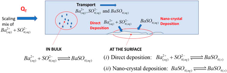
FIGURE 2. Barium sulphate precipitation and deposition mechanism.

In the calculations below, we refer to two (related) kinetic models of deposition as follows:

Model 1 refers to the case including only reactions 1 and 2 above; and

Model 2 refers to the case where all 3 reactions 1, 2, and 3 are included.

Assuming the kinetics reaction rates from the stoichiometry of the reactions in Eqs 1–3, then the kinetic equations for c₁-c₄ [representing Ba²⁺, SO₄²⁻, BaSO_4(aq) and BaSO_4(s), respectively] are as follows:

For Model 1 (reactions in Eqs 1, 2 only considered), then:

$\begin{array}{l}\frac{d{c}_1}{dt}=-k_{1f}{c}_1{c}_2+k_{1b}{c}_3\left(\mathrm{a}\right)\\ \frac{d{c}_2}{dt}=-k_{1f}{c}_1{c}_2+k_{1b}{c}_3\left(\mathrm{b}\right)\\ \frac{d{c}_3}{dt}=k_{1f}{c}_1{c}_2-k_{1b}{c}_3-k_{2f}{c}_3+k_{2b}{c}_4\left(\mathrm{c}\right)\\ \frac{d{c}_4}{dt}=k_{2f}{c}_3-k_{2b}{c}_4\left(\mathrm{d}\right)\end{array}(4)$

And for Model 2 (all 3 reactions in Eqs 1–3), then:

$\begin{array}{l}\frac{d{c}_1}{dt}=-k_{1f}{c}_1{c}_2+k_{1b}{c}_3-k_{3f}{c}_1{c}_2+k_{3b}{c}_4\left(\mathrm{a}\right)\\ \frac{d{c}_2}{dt}=-k_{1f}{c}_1{c}_2+k_{1b}{c}_3-k_{3f}{c}_1{c}_2+k_{3b}{c}_4\left(\mathrm{b}\right)\\ \frac{d{c}_3}{dt}=k_{1f}{c}_1{c}_2-k_{1b}{c}_3-k_{2f}{c}_3+k_{2b}{c}_4\left(\mathrm{c}\right)\\ \frac{d{c}_4}{dt}=k_{2f}{c}_3-k_{2b}{c}_4+k_{3f}{c}_1{c}_2-k_{3b}{c}_4\left(\mathrm{d}\right)\end{array}(5)$

The terms in red in Eq. 5 are the kinetic terms arising from the additional direct barite deposition reaction in Eq. 3. This system of Ordinary Differential Equations (ODEs) must be solved to obtain the concentration of each species over time. However, as in all consistent sets of chemical reaction, the steady-state reached by the kinetic system must of course be the equilibrium state of the set of Eqs 1–3. The constraints in this system of both equilibrium and kinetic equations are explained in Supplementary Appendix SA.

The reactive transport system—reaction-diffusion-advection

The coupled reactive transport model

To describe the full physics and chemistry of the barite deposition for a system in laminar flow it is necessary to couple the bulk chemical reaction (Eq. 1), the surface reactions (Eqs 2, 3) with the Stokes flow equation. In the simpler flowing case, these equations must be solved in a fixed geometry, e.g., a pipe, a constriction, a valve, etc. However, in a more realistic system with barite deposition (or the deposition on any solid), this deposition can change the flow geometry dynamically. Thus, in the general case our simulation model must be able to accommodate the “deforming geometry” of the system. In this work, this is achieved by using the multi-physics flow model COMSOL5.6, which can model all aspects of this reacting and dynamically evolving system. Supplementary Figure SA6 of the Supplementary Information shows the relation between the various parts of the coupled physics. The bulk reaction uses the velocity field from the Stokes equation. Once the aqueous phase barite reaches the reaction site, the tube wall reacts and converts to immobile barite as a solid phase. This immobile solid deposited barite causes the geometry to change, and the deforming geometry gridding module in COMSOL solves this change. Since the flow path changes because of changing geometry, the flow field is then solved again in the next time step.

Stokes flow

In simulating the flow field, we used Stokes flow rather than the complete Navier-Stokes equation. Stokes flow neglects the inertial term within the momentum equation and is useful for lower Reynolds number laminar flows. In Eq. 6, u is the velocity field, $\rho$ is the density of the fluid, K is the viscous force tensor, and F is a volumetric force tensor and Eq. 7 is the continuity equation assuming the fluid in incompressible.

$\rho \frac{\partial \mathbf{u}}{\partial t}=\nabla \cdot \left[p\mathbf{I}+\mathbf{K}\right]+\mathbf{F}(6)$

$\rho \nabla \cdot \mathbf{u}=0(7)$

The inlet boundary conditions is defined by the mass inflow for a mixture of barium and sulphate ions in solution, and the formulation is as follows in Eq. 8:

$-\int \rho \left(\mathbf{u}\cdot n\right)d\mathrm{\Omega }=m(8)$

where $\mathrm{\Omega }$ is the surface integration operator.

The outlet boundary condition in shown in Eq. 9 where p₀ is the defined outlet boundary pressure, which is atmospheric in our calculations, p is the pressure, and K is the viscous force.

$\left[-p\mathbf{I}+\mathbf{K}\right]\mathbf{n}=-p_0\mathbf{n}(9)$

Aqueous phase transport

Equation 10 shows the advection-diffusion-reaction partial differential equation (PDE) that governs the bulk aqueous phase transport in which c_i is the species i concentration in mol/m³. Eq. 11 gives the expression for J_i, which is the diffusive flux of species i in mol/m².s, u is the velocity field in m/s. Eq. 12 shows the expression for the boundary condition at the outlet, and n refers to the normal vector in the outlet boundary, D_i is the diffusion constant in m²/s, and k is the related reaction rate constant. In the rate Eq. 12, v is the stoichiometric coefficient, which is 1 for reactants and −1 for products, in all the reactions modelled here.

$\frac{\partial c_i}{\partial t}+\nabla \cdot {\mathbf{J}}_i+\mathbf{u}\cdot \nabla c_i=R_i(10)$

${\mathbf{J}}_i=-D_i\nabla c_i(11)$

$n\cdot D_i\nabla c_i=0,outletboundarycondition(12)$

The diffusion coefficient used in this numerical simulation is D = 1e-8 m²/s.

Surface reaction/barite deposition

The “surface reaction” is the deposition of the transported nano-crystals of barite [denoted as BaSO_4(aq)] (Eq. 2) or by direct deposition from reaction of the free ions (Eq. 3). The formulation of the surface reaction is shown below in Eqs 13, 14.

$\frac{\partial c_{s,i}}{\partial t}=R_{s,i}(13)$

$R_{s,i}=v_i\cdot k_s\prod _{i\in react}{c}_{s,i}(14)$

The coupling between surface reaction and bulk reaction, discussed under the Aqueous phase transport section, is implemented as a normal flux out of the flowing system onto the surface. This flux out of the system would only be diffusive in laminar flow. Eq. 15 shows the boundary condition used for coupling reaction in the bulk phase and reaction on the surface, where k_s is the surface reaction constant. Eq. 15 considers diffusion in directions x, the principal flow direction, and y, transverse to the flow direction onto the wall. In the advection dominated systems where flow is in the x-direction, we can often ignore the derivative of concentration in the x-direction although we are accounting for it in all of the numerical modelling results.

$D_i\left(\frac{\partial c_i}{\partial x}+\frac{\partial c_i}{\partial y}\right)=k_{s}c(15)$

Diffusion penetration length, δ

Since the only mechanism for the deposition on the surface in laminar flow is through the normal diffusive flux, it is important to understand the extent of this near surface diffusive zone. It was noted above that under advection domination we can often ignore the derivative of concentration in the x-direction. In the analytical development below, we will assume $\left(\frac{\partial c_i}{\partial x}\right)\ll \left(\frac{\partial c_i}{\partial y}\right)$ in order explain the behaviour of the system under different depositional regimes, in particular we discuss the concept of the diffusion penetration length, δ.

To define δ, we use the transport terms of Eq. 6 at steady-state conditions where the diffusive fluxes in Eq. 16 are shown in Eq. 17, as follows:

$\nabla \cdot {\mathbf{J}}_i+\mathbf{u}\cdot \nabla c_i=0(16)$

$J_i=-D_i\nabla c_i=D_i\left(\frac{\partial c_i}{\partial x}+\frac{\partial c_i}{\partial y}\right)(17)$

In Eq. 17, we assume that the advection is dominant in the x-direction, and thus, we can remove the diffusive flux in the x-direction. Hence, from Eq. 16 the diffusion penetration length, δ, can be derived as shown below in Eqs 18, 19:

$-D_i\left(\frac{c_i}{y^2}\right)+u\left(\frac{c_i}{x}\right)=0(18)$

$\mathrm{w}\mathrm{h}\mathrm{i}\mathrm{c}\mathrm{h}\mathrm{i}\mathrm{m}\mathrm{p}\mathrm{l}\mathrm{i}\mathrm{e}\mathrm{s}\Rightarrow y\left(x\right)=\sqrt{\frac{D_{i}x}{u}}=\delta \left(x\right)(19)$

This length, δ, (which is a function of distance along the tube, x), is the extent that fluid in bulk can “feed” the surface reaction. To illustrate the significance of this quantity, we will bring forward an example calculation in a long tube of radius 2.5 mm. In this calculation, we assume the Model 1 kinetics where only the reactions in Eqs 1, 2 occur; i.e., Eq. 1 = the formation of the barite nanocrystalline material (BaSO_4(aq)) followed by, Eq. 2 = the deposition of the nanocrystals on the surface to form BaSO_4(s). As shown above, the second reaction only occurs at the surface as described by Eqs 13, 14, where the surface reaction rate constant is k_s. Figure 3A shows the concentration profiles of BaSO_4(aq) at two different locations along the length (x) of the pipe cross-section, at x = 5 mm and x = 15 mm as shown in Figure 3E, along with the velocity profile. The “arc length” here is the distance along the pipe diameter, and the walls are at 0 and 5 mm on the x-axis in Figures 3A, B which show the profiles of BaSO_4(aq) across the tube for no surface reaction (k_s = 0) and with surface reaction (k_s ≠ 0), respectively. Note that in Figure 3A (no surface reaction), the concentration near the walls is high because of the high residence time spent there due to the low fluid velocity (shown). Also, in Figure 3A it is found that the BaSO_4(aq) concentration is low in the pipe centre because of the lower residence time at the centre of the tube. The case where the surface reaction happens on the walls (k_s ≠ 0) is shown in Figure 3B. In this case, the BaSO_4(aq) concentration near the walls falls to nearly zero, and we observe clear maxima in the concentration profiles, as seen in this figure, and this predicted behaviour is even more unusual. This predicted unusual BaSO_4(aq) profile has not previously been reported. The location of the maximum in a particular concentration profile for the system with a surface reaction (k_s ≠ 0) marks the boundary between the zone that the diffusion penetration length controls the surface reaction rate and the area near the middle of the pipe, which is advection dominated. The diffusion penetration length, δ, is the distance between this concentration maximum and the wall where deposition is occurring. Eq. 19 above indicates that this penetration length increases with distance (x) travelled along the pipe, where δ ∼ x^1/2, and we have confirmed numerically that this is case. Figures 3C, D show the effect of the diffusion coefficient on diffusion penetration length. We can observe that at the same location in the tube, the behaviours of the concentration curves differ. In higher diffusion, we cannot see the maximum in the smaller flow rate as opposed to what we observe for the smaller diffusion coefficient. In Figure 3D the diffusion penetration length for smaller flow rates is large, so more of the nanocrystalline or “aqueous” barite [BaSO_{4 (aq)}] will be involved in surface reaction. In Figure 3C, the diffusion penetration length is smaller so we can observe that beyond that length, the concentration of BaSO_{4 (aq)} becomes higher. Experimental evidence will be presented below to support these modelling predictions.

FIGURE 3

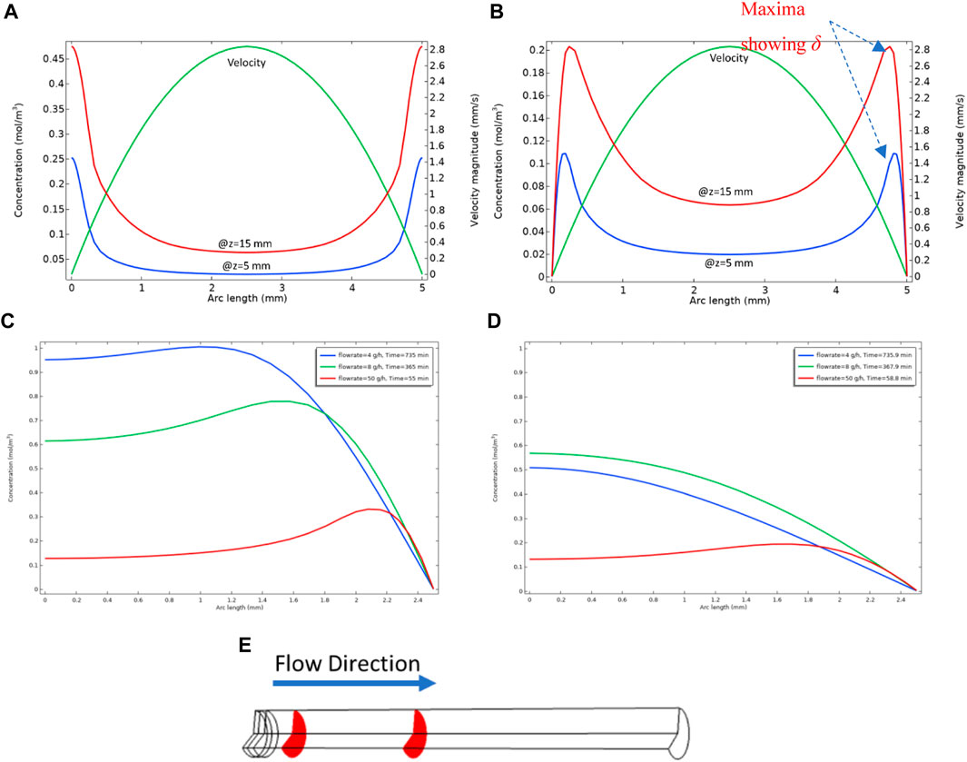
FIGURE 3. (A) Concentration of BaSO_4(aq) in bulk WITHOUT surface reaction (k_s = 0) in the planes shown in (E) with diffusion coefficient = 1e-8 m²/s, (B) shows the concentration of BaSO_4(aq) WITH surface reaction (k_s ≠ 0) in the planes shown in (E) with diffusion coefficient = 1e-8 m²/s, (C) BaSO_{4 (aq)} concentration profile at z = 15 mm with diffusion coefficient = 1e-9 m²/s, showing centre of the tube (x = 0) to the wall (x = 2.5 mm) on x–axis (D) BaSO_{4 (aq)} concentration profile at z = 15 mm with diffusion coefficient = 1e-8 m²/s, showing centre of the tube (x = 0) to the wall (x = 2.5 mm) on x–axis, (E) Tube used for numerical experiments, the red planes show x = 5 mm and x = 15 mm. The plots show steady-state condition.

Surface Damköhler number

We have discussed in the previous section that the primary mechanism of the surface reaction and subsequent deposition is the normal diffusive flux, which is effective within the reach of the diffusion penetration length, δ. We now establish the conditions under which the surface reaction or bulk diffusion dominates the surface reaction mechanism.

A surface Damköhler number, $D{a}_s$, can be derived based on the boundary condition that couples the reaction in bulk and the surface reactions in Eq. 15. A dimensional analysis on this boundary condition is carried out to derive the surface Damköhler number.

Assuming that the dominant diffusive flux occurs in the normal (y) direction to the flow direction (x), then Eq. 15 may be written as Eq. 20a. Define $\theta$ and $\overline{y}$ as dimensionless concentration and length as shown in Eqs 20b, c. Then, by substituting these quantities in Eq. 20a, we arrive at Eq. 20d. The dimensionless coefficient on the RHS of Eq. 20d is then defined as the surface Damköhler number, $D{a}_s$, as in Eq. 20e.

$\begin{array}{l}{D}_i\left(\frac{\partial c_i}{\partial y}\right)=k_{s}c\left(\mathrm{a}\right)\\ \theta =\frac{c}{c_0}\left(\mathrm{b}\right)\\ \overline{y}=\frac{y}{L}\left(\mathrm{c}\right)\\ \frac{d\theta }{d\overline{y}}=\frac{k_{s}L}{D}\theta \left(\mathrm{d}\right)\\ D{a}_s=\frac{k_{s}L}{D}=\frac{surfacereactionrate}{bulkdiffusionrate}\left(\mathrm{e}\right)\end{array}(20)$

The surface Damköhler number is the ratio of surface reaction rate to the diffusion rate within the diffusion penetration length, δ, implying that L∼ δ in Eq. 20c. That is, if Da_s > 1, then the deposition is surface controlled and if Da_s < 1, then the deposition is diffusion controlled. In very high Damköhler numbers, Da_s >> 1, the deposition remains almost the same, even for very high k_s values, because the diffusion penetration length limits the extent of the reaction.

Results and discussion for the constant rate simulations and experiments

Input data for simulation

As the simplest approach to model the deposition of barium sulphate, we will consider the depositional process at the walls of the tube at a constant flow rate, firstly with no change in the geometry of the system. We performed these calculations for the various cases in Table 1 for the injection of 50 control volumes (control volume = flowrate*time/tube volume).

TABLE 1

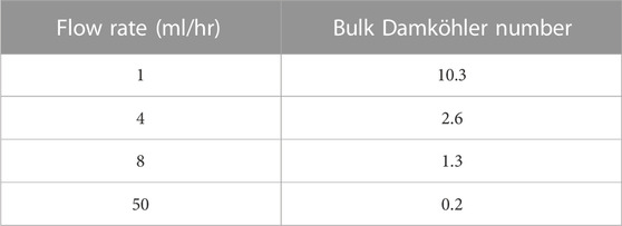
TABLE 1. Flow rate and Bulk Damköhler number in the constant flow rate study.

We performed the simulation in a simple tube with a diameter of 5 mm and length of 50 mm.

To solve the ODE system of Eqs 4, 5, we need a set of reaction kinetics constants. We used the values of k_1f = 2E-3 m³/(s.mol), k_1b = 1E-9 1/s, k_2b = 1E-7 1/s as tabulated in Supplementary Table SA2 of the Supplementary Information. We used a random reaction kinetics constant for reaction 2 in Eqs 4, 5 to replicate the inconsistency of the suitable deposition sites along the deposition surface, as presented in Supplementary Figure SA5 of the Supplementary Information. Simulations were performed for the mechanisms in both Model 1, i.e., deposition through an intermediate species of BaSO_4(aq), and Model 2, i.e., through direct deposition as well as through an intermediate phase. We chose three different values of k_3f = 1E-8, 1E-6, and 1E-4 m⁴/(s.mol); these values show an intermediate deposition dominated, a balanced deposition rate between the two mechanisms, and a direct deposition dominated regime, respectively.

Following the constant flow rate examples, a calculation is presented for a “ramped” flow rate from a low to a high value. In the changing flow rate case, we ramped the flow rate linearly over time from 1 ml/h to 100 ml/h in 4,000 min in this case, as presented in Figure 4. As a result of this increase in flow rate, the bulk Damköhler number [Da_bulk = k_1f*C_Ba,0/volumetric flow (Fogler, 2010)] decreases from 10.32 to 0.10. This slow flow rate implies that the reaction governs the system initially, and as the flow increases, advection replaces the reaction as the governing mechanism.

FIGURE 4

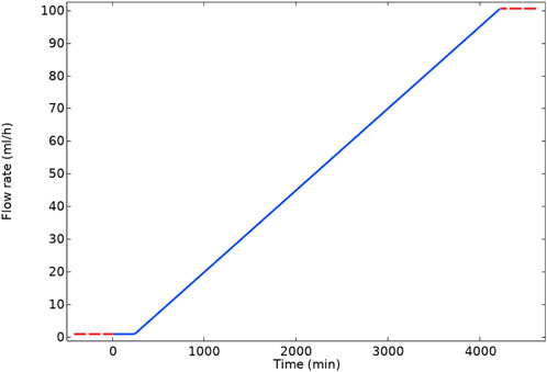
FIGURE 4. Flow rate ramp with time.

We can also calculate the equilibrium constant $\stackrel{\sim }{K}$ in each case $\stackrel{\sim }{K}=k_f/k_b$. (Values of $\stackrel{\sim }{K}$ in Supplementary Appendix, plus derivation of k_3b). We also used a diffusion coefficient of D = 1e-8 m (Fu et al., 2012)/s.

Wall deposition of barite with constant flow

This set of calculations is presented to identify the behaviour of a reactive transport system in the case of constant flow rate (no geometry change due to deposition), for the Model 1 and Model 2 kinetic deposition models. This case is not completely realistic in that flow velocity changes occur if any deposition/blockage forms and this is not (yet) accounted for. However, the constant flow rate/no geometrical deformation cases provide valuable information that assists in the explanation of the ramp-up and deforming geometry cases. Detailed discussion of this topic can be found in supporting information accompanied with this paper.

Since the detailed numerical results reported below are quite complex, we anticipate our findings by explaining the main observations from the Model 1 and Model 2 simulations.

1. At the lower flow rates, the residence time is high thus a high percentage of reactants (i.e., barium and sulphate in this study) convert to aqueous barite, [BaSO_4(aq)].

2. In addition, at low flow rates, the diffusion penetration length (δ) is relatively large; for example, at the volumetric flow rate of 1 ml/h, the diffusion penetration length is larger than the tube radius or channel width.

From the points above, we note there is more material being produced in the system through reaction at lower flow rates. However, due to the hydrodynamics of the system (the large diffusion penetration length), the surface consumes much or almost all of that material. That is, most of this deposition happens near the inlet of the tube due to the kinetics/hydrodynamics of the system. At higher flow rates, the deposition location moves gradually towards the outlet end of the tube. The increasing flow rate reduces the residence time and thus there is more material for deposition further along the tube near the end. Also, at higher flow rates, the diffusion penetration length, δ, also decreases which leads to lower absolute mass deposition of barite (per volume throughput) on the surfaces.

Barite deposition pattern using Model 1—constant flow rate

Figure 5 shows the surface barite deposition rate for a range of flow rates for Model 1; i.e., including the kinetic reactions in Eqs 1, 2 only. In this example, for simplicity of interpretation, we take the kf2 value as being constant, rather than being variable as shown in Figure 3A. It is observable from Figure 5 that in the lower flow rates, most of the deposition occurs near the inlet of the tube when we inject 50 control volumes. This deposition pattern near the inlet at lower flow rates is a consequence of the Model 1 reaction mechanism, i.e., first BaSO_4(aq) formation and subsequent deposition at the surface. The surface reaction consumes BaSO_4(aq) produced in bulk near the inlet, and lower BaSO_4(aq) will remain in the system for transportation further down the tube and subsequent deposition. At higher flow rates, the residence time is shorter in the system. Thus, for the deposition to happen, 1) it takes more time for the bulk reaction to produce BaSO_4(aq) and 2) the bulk fluid transports BaSO_4(aq) further down the tube where higher levels of deposition subsequently occur.

FIGURE 5

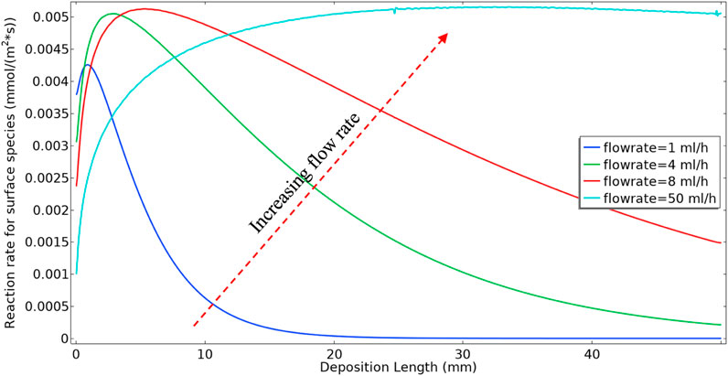
FIGURE 5. Deposition rate in constant flow rate approach.

Figure 6 shows the volume-averaged concentration of BaSO_4(aq) in the bulk phase. In these calculations, the surface reaction is “switched on” after injecting 2 control volumes of the reactants into the cell. The calculation was performed in this manner to establish a simplified initial condition with the system full of input Ba²⁺, SO₄²⁻ and BaSO_4(aq), with no surface deposition. The results in Figure 5 show that the behaviour of the final average value of BaSO_4(aq) in the system is not monotonic. At lower flow rates, because of higher residence time, there will be more production of BaSO_4(aq) in bulk. Also, for lower flow rates, the diffusion penetration length is more extensive. Thus surface reaction can consume nearly all BaSO_4(aq) in bulk at the slowest flow rate, i.e. 1 ml/h. At the highest flow rate, i.e. 100 ml/h, 1) the residence time is much lower, which results in a smaller production of BaSO_4(aq), and 2) the diffusion penetration length is smaller than at lower flow rates; thus, surface reaction consumes a smaller fraction of the BaSO_4(aq). However, it is evident that there is a balance between the two effects of residence time and diffusion penetration length, which in this case, leads to the greatest mass of BaSO_4(aq) being generated at 8 ml/h, and a lesser amount at the higher flow rate of 50 ml/h.

FIGURE 6

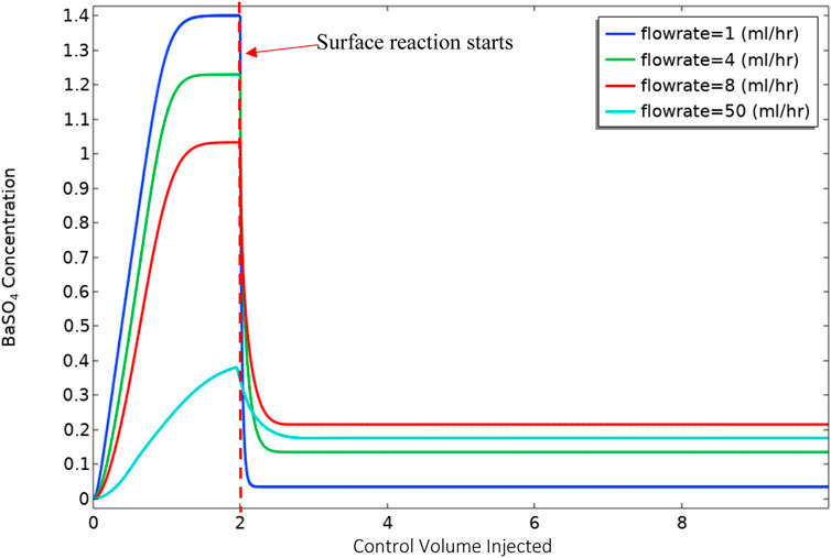
FIGURE 6. Volume-averaged BaSO_4(aq) concentration versus control volume injected.

Figure 7 shows the barite deposition in mg of BaSO_4(s) per 10 mm section along the system for the 8 and 50 ml/h cases after the same total volume throughput (50 control volumes). Clearly, (i) in the lower 8 ml/h flow rate case, the absolute deposition of BaSO_4(s) is much higher, it is highest closer to the inlet and it then decreases along the system; and (ii) in the higher 50 ml/h flow rate case, the deposition of BaSO_4(s) is much lower overall, it is lower closer to the inlet and it then increases along the system. This has already been explained by the balance of bulk and surface reactions discussed above.

FIGURE 7

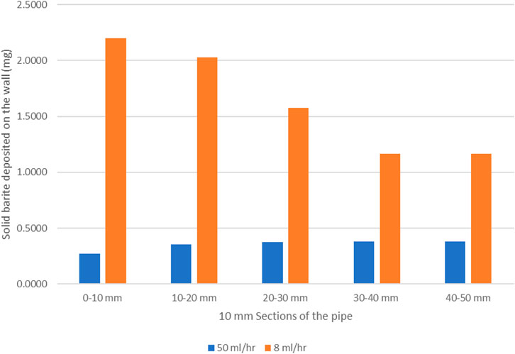
FIGURE 7. Mass of solid barite deposited on the wall as a function of distance from inlet.

Barite deposition pattern using Model 2—constant flow rate

Recall that the Model 2 formulation includes both the formation of mobile nanocrystals of barite (BaSO_4(aq)) as an intermediate form which deposits as solid barite at a surface and in addition the direct deposition of Ba²⁺ and SO₄^2- ions onto the surface (as BaSO_4(s)). This latter direct deposition includes all three kinetic Eqs 1–3, where Eq. 3 has a kinetic depositional rate constant, k_3f. In this example, both kf2 and kf3 are taken as being slightly variable as shown on Supplementary Figure SA5 of Supplementary Information, to additionally show the effects of surface property (deposition rate) heterogeneity on these constants. Figure 8 shows the surface reaction rate (deposition rate) for three kinetics values of k_3f (all slightly variable as indicated in Supplementary Figure SA5B of Supplementary Information) for this direct deposition mechanism, and these values lead to three different deposition regimes within Model 2. The smallest value, k_3f = 1e-8 m⁴/(s*mol), has a smaller deposition amount similar to Model 1 (see Figure 8A). As the value increases, there is a balanced deposition regime between the two deposition mechanisms through intermediate phase and direct ion deposition, which is the case for k_3f = 1e-4 m⁴/(s*mol) (see Figure 8B). We have also included a dominant direct deposition regime, k_3f = 1e-4 m⁴/(s*mol) (see Figure 8C). It is observable from Figure 8C that the direct deposition mechanism mostly occurs at the inlet end of the tube. The ion direct deposition mechanism has a higher rate for a higher flow rate, which is because of higher reactant throughput into the cell. The k_3f parameter depends on the surface behaviour, i.e., it would probably be a higher value for rougher surfaces. The numerical experiment with the direct deposition model provides information on how a real system might evolve under the conditions in which the ion deposition on the surface is favourable. Obviously, we would expect that surfaces that greatly enhance the direct deposition, will also lead to a blockage near the inlet of the flowing tube. This would also affect the reaction in the bulk, since the reactants that lead to mobile barite [BaSO_{4 (aq)}] are being consumed on the surface. The implication of this for the downstream would be lower deposition through the mobile barite.

FIGURE 8

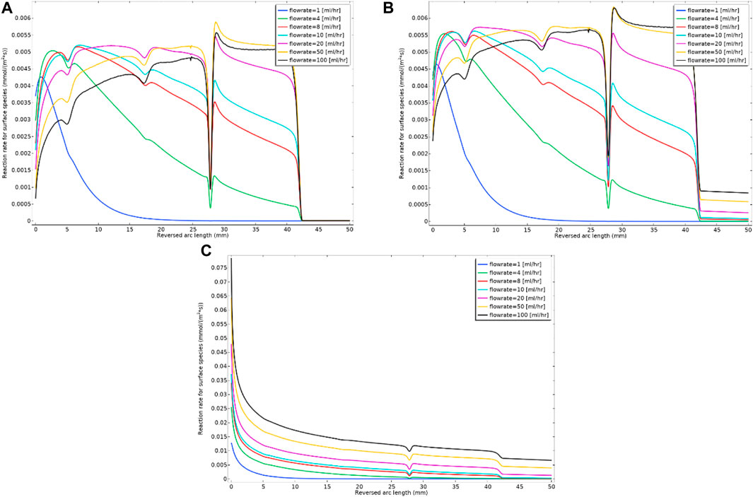
FIGURE 8. Surface reaction rate (deposition rate) for three different kinetics constants of (A) k_3f = 1e-8 m⁴/(s.mol); (B) k_3f = 1e-6 m⁴/(s.mol) and (C) k_3f = 1e-4 m⁴/(s.mol) for the constant flow rate and Model 2 kinetics.

Model 2 enhances the flexibility and accuracy of barite deposition prediction, since it accounts for both possible mechanisms of direct surface deposition from the bulk (Eq. 3) as well as via the intermediate nanocrystal deposition (Eq. 2). If the surface is not rough, Model 1 might be sufficient to calculate the deposition rate (as shown in Figure 8A) and the calculation degrees of freedom would be reduced to account for a new reaction, i.e., direct ion deposition.

As the deposition takes place in the system, the geometry of the system should change as the tube becomes blocked. Thus the constant flow rate approach may address the initial reaction and the deposition in the system. However, it does not consider the hydrodynamic changes in the system caused by the tube becoming constricted. Obviously, these constrictions affect both the residence time in a given section of the tube and also the diffusion penetration length. This will be addressed later in this paper, where deformed geometry is used to model all aspects of these changes.

Comparing the constant flow rate experiments with simulation

The barite deposition in channel experiments

Before making a direct comparison with the channel experiments in which barium and sulphate ions are mixed at the inlet of a channel, we describe the experimental set up. Figure 9 shows the configuration of the flow channel (working section, length L = 120 mm; width, W = 3 mm) and the design of the inlet mixing assembly, which is required to obtain good (but not complete) mixing near the inlet. The two reactants are being injected from two separated inlets at a constant flow rate, thus the viscous layers’ behaviour is an impedance to the perfect mixing in the vicinity of the inlet; this can be observed experimentally in Figure 9B.

FIGURE 9

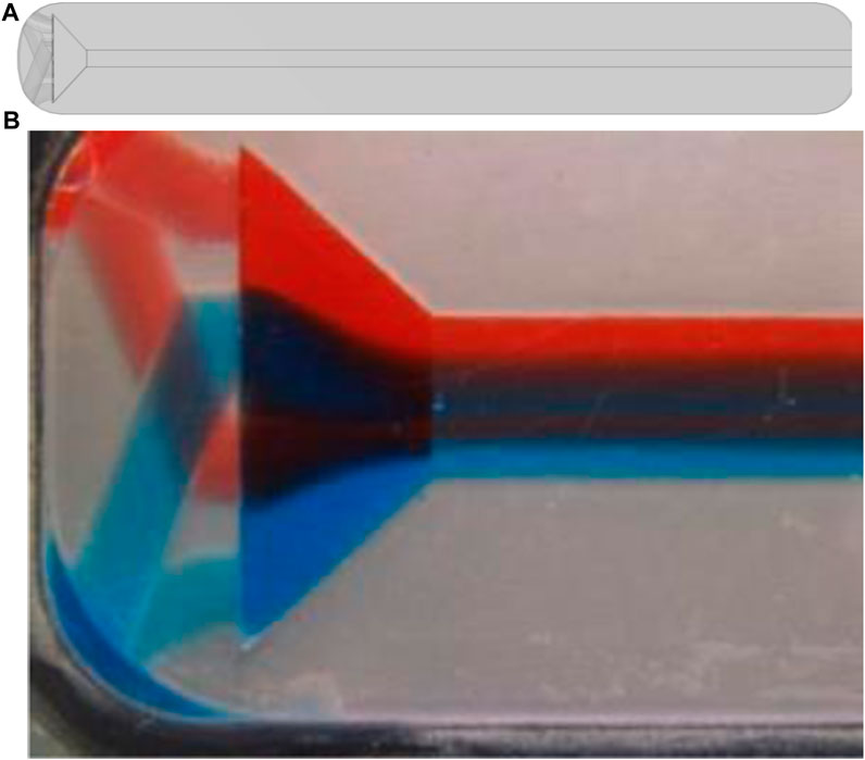
FIGURE 9. (A) Experimental setup for simple flow channel with four inlets to achieve more mixing in the channel, (B) dye experiment to show mixing.

We replicated the same behaviour of mixing by simulating the laminar flow, using the Navier-Stokes equations, which can be seen in Figure 10A. This will enable us to have a closer look at the concentration profiles within the cross-section of the experimental setup. The cross-section is particularly important as diffusive flux is the dominant means of mass transport to the walls in the laminar flow regime. We can observe from Figure 10Aiv that full mixing is not completely taking place. The same behaviour can be observed in the experiment with reactants in Figure 10B where we can track the plume of high concentration barite inside the two dotted areas.

FIGURE 10

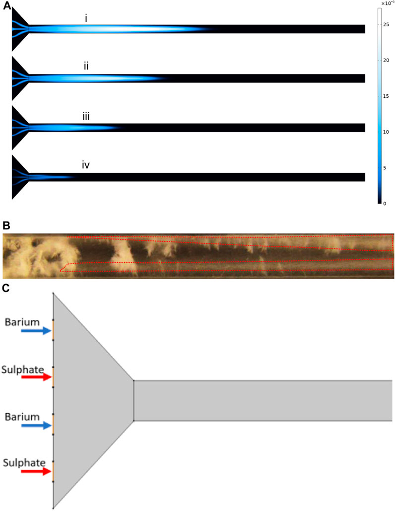
FIGURE 10. (A) BaSO_{4 (aq)} concentration profile at different time steps at flow rate of 8 ml/h. (B) The cloudiness showed by the dotted lines represents BaSO(aq). (C) The schematic of thesimulation showing inlet positions for Barium and Sulphate.

To further understand the concentration distribution in the cell cross-section, we extracted the concentrations from the simulation which is represented in Figure 11. Figure 11A shows the cross-sections that are used to plot the concentrations. The actual concentration profiles are shown in Figure 11B. These concentration profiles are important to further understand the effect of diffusion penetration length and the extent that the bulk material can feed the surface reaction. It can be seen that near the inlet of the tube, there are two peaks in the concentration which are analogue to what is observable in Figure 10B. That is, enclosed “hazy” dotted areas in Figure 10B are identified as regions of the species BSsO_4(aq)—the intermediary form of barite - which is actually transported through the system.

FIGURE 11

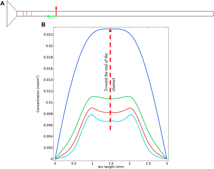
FIGURE 11. (A) Location of the cross sections in the simulation geometry. (B) Cross sectional concentration profile.

Diffusion penetration length from formula

The diffusion penetration length is given by Eq. 19 above; i.e., $\delta \left(x\right)=\sqrt{\frac{D_{i}x}{u}}$. By using this equation, we can calculate the diffusion penetration length for flow rates of 8 and 50 ml/h, as shown in Figure 12. We can approximately calculate the diffusion penetration length from experiment shown in Figure 13. In Figure 10B, as noted above, we interpret the cloudiness near the wall–which appear like “vapour trails”—to represent the diffusion penetration length. This feature (the “vapour trails”) have appeared in almost all of our flow experiments in channels for barite deposition. The measurements in Figure 10B indicate that the diffusion penetration length is approximately, δ∼0.64 mm which is in good agreement with the calculated value from Eq. 19 which is δ∼0.7 mm. A video of this experiment is available in supporting information which shows the dynamic development of the “vapour trails” and also the subsequent deposition of barite (see deposition_video.mp4 in the Supplementary Appendix SB).

FIGURE 12

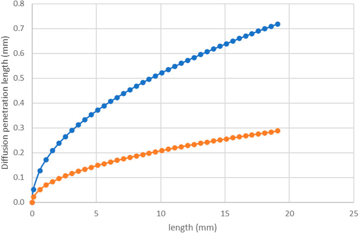
FIGURE 12. Diffusion penetration length, δ vs. distance along the tube (x) calculated using Eq. 19 for 8 ml/h (orange line) and 50 ml/h (blue line).

FIGURE 13

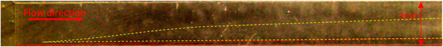
FIGURE 13. Deposition in simple channel experiment (L = 30 mm of 120 mm total length, W = 2 mm).

Figure 13 shows a frame of the experiment in which two different regions are defined. The region defined by yellow dotted line represents a plume of high concentration BaSO_{4 (aq)} we can observe from the figure that this region does not penetrate the red region despite its high concentration. As shown and discussed in Figure 11B, due to the type of flow and the diffusion transport mechanism, the bulk concentration cannot feed the surface after a particular length that is diffusion penetration length: this diffusion penetration length is defined by the red dotted line in Figure 13.

Figure 14 shows the cumulative consumed barium from experiment and model. We used ICP analysis to measure the barium concentration in the effluent of the experimental cell. The diagram shows that the barium sulphate reaction rate kinetics constant in this case lies between 1.4e-4—0.002 m³/mol/s, showing that the modelling procedure is in reasonable semi-quantitative agreement with the experimental observation.

FIGURE 14

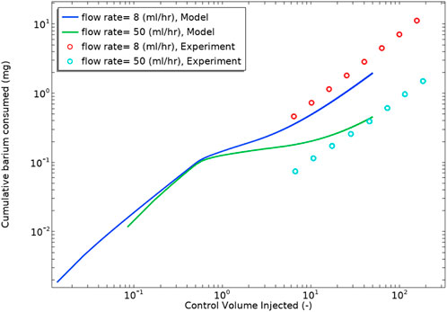
FIGURE 14. Cumulative consumed barium derived from experiment and modelling vs. control volume injected. The Saturation Index of the brine used is 3.4.

The mixing pattern is also observable from the numerical simulations. In the experimental setup, the barium is flowing from the top inlet (indicated as red in Figure 9B), and the sulphate is flowing from the bottom (indicated as blue in Figure 9B).

Figure 15 shows the cumulative deposited barite on the top and bottom surfaces. It can be observed that the total deposited barite is higher on the top surface which is closer to the barium plume. Since the barium is the limiting reactant here, the deposition is higher where its concentration is higher.

FIGURE 15

FIGURE 15. Cumulative deposited barite on the top and bottom of the flow channel.

In summary, the main conclusions from the steady-flow unsteady-state simulations and experiments are as follows:

1. In the coupled simulation of the flow and mass transport, there are two boundary layers which are of importance to consider:

a. The hydrodynamic boundary layer which is a narrow region near the wall where flow is theoretically zero.

b. The diffusion penetration length as identified in Eq. 19 that defines the effective mass transfer length in the laminar flow.

2. The deposition process will change the mixing behaviour near the wall and in the bulk by changing the geometry and local residence times. It is therefore important to take into account the deformations which we will address below.

3. At low flowrates, the deposition will take place near the inlet vicinity and as the flow rate increases the deposition location moves to the end of the tube.

Deposition on the wall with changing flow and explicit inclusion of the depositional geometry

In this section, we now build on the previous work described above in two major ways, as follows:

(i) We allow the deposition of barite at the channel surface to cause a constriction which we model using a deformable grid. As a consequence of the channel constriction (being variable along the system) this changes the local flow rates at different points in the channel, and

(ii) We model a “ramped flow” as described in Figure 4 where the total flow rate also changes from a low value to a high value over time.

Although this system is quite complex and several interaction processes are occurring at the same time, some definite observations and predictions are made from the observed results. In addition, this is much more like a real field system (e.g., in a wellbore or pipe) where barite deposition may typically be taking place.

As mentioned earlier, the barium and sulphate ions and mobile barite [BaSO_4(aq)] deposit on the surface within reach of diffusion penetration length, δ, as described by Eq. 19. δ depends on the velocity and the longitudinal length in the system; for example, our derivation shows that δ grows as $\sqrt{x}$ along the tube. As the deposition process takes place, the hydrodynamic state of the system changes its behaviour since the barite deposit will shrink the system volume and thus flowing area. This will, in turn, affect the reaction ions (Ba²⁺ and SO₄²) residence time and also the available surface for deposition. This change in residence time and available reactant surface feeds back into the reaction, thus changing the deposition behaviour. So it is vital to investigate this “feedback” behaviour arising from the complex coupled effects of a changing flow rate on the deposition behaviour.

As a result of the increase in the flow rate over the ramped period, the diffusion penetration length decreases, as described by Eq. 19, and this change is shown in Figure 16A for different flow rates. Figure 16B shows BaSO_4(aq) concentration in the bulk phase in the channel cross-section at z = 10 mm. As mentioned previously, we include the surface deposition reaction after the bulk reaction is at a steady state. Thus, before the surface reaction occurs, the system is filled with BaSO_4(aq) as seen at t = 100 min in Figure 16B. Once the surface reaction occurs and the diffusion penetration layer establishes and then the surface reaction starts to consume BaSO_4(aq) within the reach of the (now changing) diffusion penetration length.

FIGURE 16

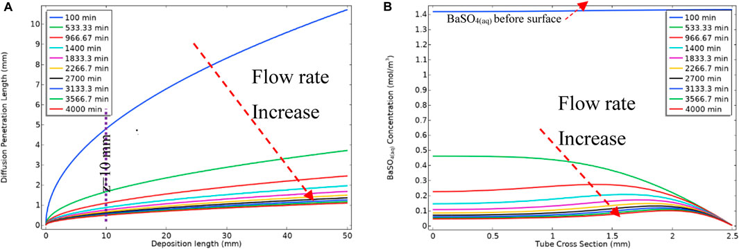
FIGURE 16. (A) Diffusion penetration length vs. the deposition length at different time steps (B) Concentration of BaSO_4(aq) at z = 10 mm cross-section of the tube.

Deposition pattern for the changing flow rate case for Model 1

Figure 17 shows the surface reaction (deposition) rate along the surface. The green curve, at 533.33 min, is showing the deposition along the surface for the high bulk Da number, which is equivalent to a slow flow rate. It is observable that most of the deposition at this state is happening at the tube inlet. As we decrease the bulk Da number (by increasing the flow rate), the deposition rate decreases at the inlet end of the cell and increases at the outlet of the cell. This change in deposition location is because the deposition mechanism is through the deposition of the intermediate barium sulphate phase, i.e., BaSO_4(aq). As the flow rate increases, 1) the residence time decreases, so less reaction time is available for the BaSO_4(aq), and 2) the fluid transports the “intermediate” BaSO_4(aq) further down the tube and more deposition the occurs in that location.

FIGURE 17

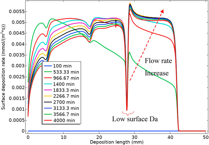
FIGURE 17. Surface deposition rate vs. the deposition length.

Figure 18 shows the volume-averaged concentration of BaSO_4(aq) over the bulk and surface averaged deposition rates and deposited mass over the depositing surface. Once the surface reaction starts (indicated in Figure 18), the amount of BaSO_4(aq) drops sharply. This sharp drop, as indicated in Figure 16A, occurs since the diffusion penetration length at the low flow rate is larger than the tube diameter, and surface reaction consumes virtually all of the BaSO_4(aq). Hence, the BaSO_4(aq) concentration then settles at a constant value until the flow rate ramp starts. Once the flow rate ramp starts, the BaSO_4(aq) concentration in bulk starts to increase until a bulk Damköhler number of around 1. This increase in the BaSO_4(aq) concentration is then observed for the following reasons:

1) There is more reactant throughput into the tube while the bulk governing mechanism is still reaction dominated.

2) The diffusion penetration length is becoming smaller (because of the higher flow rate), limiting the consumption of BaSO_4(aq) by the surface reaction. From a bulk Damköhler number of 1 onwards (green circle in Figure 18), BaSO_4(aq) concentration starts to drop. This reduction in the BaSO_4(aq) concentration is because the reaction mechanism in bulk is becoming advection dominated, so despite the smaller diffusion penetration layer, BaSO_4(aq) drops due to lower residence time. This drop continues until it settles at a constant flow rate. The deposition rate also becomes slower (the yellow circle in Figure 18) as the system moves into a highly advection dominated regime.

FIGURE 18

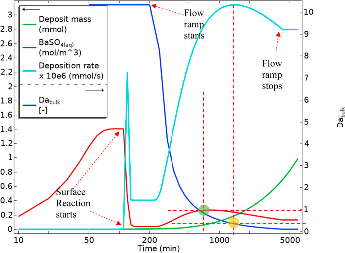
FIGURE 18. Average quantities of BaSO_4(aq) in bulk, Deposition rate on the surface, Deposit mass, and Bulk Damköhler number in Model 1.

Deposition pattern for the changing flow rate case for Model 2

Figure 19A shows the surface deposition rate using Model 2 in a regime where deposition through the intermediate phase is dominant. This difference in deposition regime is observable by comparing Figures 5, 8A, and the same discussion for Model 1 applies here. Figure 19B, however, is within a balanced deposition regime, as explained earlier. In a deposition regime through an intermediate phase of BaSO_4(aq), see Figures 17, 19A, the deposition rate reduces at the inlet of the tube as the flow rate increases. However, in a balanced deposition regime of through intermediate and direct deposition, the deposition rate at the tube’s inlet remains almost the same during the flow ramp up because the barium and sulphate ions are constantly replenishing into the tube they directly deposit on the surface. In a highly direct deposition dominated environment, as in Figure 19C, most of the deposition occurs at the beginning of the cell.

FIGURE 19

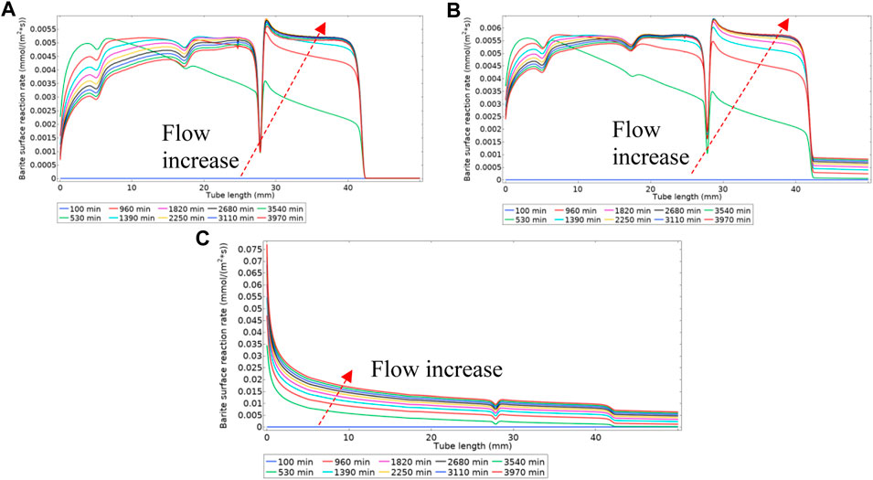
FIGURE 19. Surface reaction rate (deposition rate) for three different kinetics constants of (A) k_3f = 1e-8 m⁴/(s.mol) (B) k_3f = 1e-6 m⁴/(s.mol) (C) k_3f = 1e-4 m⁴/(s.mol).

Figure 20 gives a volume-average and surface-average of the bulk and surface reaction versus time. This figure shows the averaged values for three different k_3f (surface reaction constant) in the three regimes discussed earlier. The discussion for Figure 18 also applies here for the concentration of BaSO_4(aq), bulk Damköhler number, and the mass deposited. Deposition rates for three different deposition regimes, shown as dashed lines in Figure 20, show the balance between the deposition through an intermediate and direct deposition. The blue dashed curve in Figure 20 shows the intermediate dominated deposition regime, and the deposition curve has a maximum that shows the advection is governing the deposition at this stage. In the two other curves, dashed green and dashed red, the deposition rate increases until the flow ramp up stops. This deposition behaviour is because the primary deposition mechanism is through direct ions deposition on the surface, as shown in Figures 19B, C.

FIGURE 20

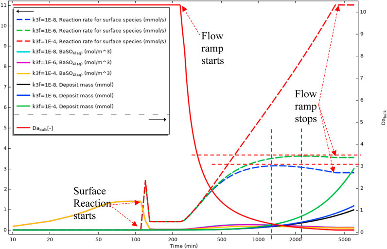
FIGURE 20. Average quantities of BaSO_4(aq) in bulk, Deposition rate on the surface, Deposit mass, and Bulk Damköhler number in Model 2.

Deposition pattern for the changing flow rate/changing geometry case for Model 1

Thus far in this paper, we have tried to isolate the various individual aspects of the dynamics in the barite depositional system, and then attempt to interpret their interplay. In the previous cases, the bulk reaction, the surface reaction, and the flow rate ramp-up start in sequence to investigate the effect of each individual aspect of the physics in the system. In this case, all of the various parts of the physics now occur simultaneously from the start of the simulation. We then try to interpret the results and findings based on the previous discussions.

In this case, we also change the tube geometry based on the mass of solid deposits on the surface. In this work, we consider the change in the geometry as a reduction in the channel width, and no flow can pass through the deposit itself (it is impermeable). As the geometry changes, the flow field changes and this impacts on the transport equation.

Figure 21 shows BaSO_4(aq) averaged values in bulk, the mass deposited, the deposition rate, and the bulk Damköhler number versus time. It is observable that the BaSO_4(aq) concentration decreases as the surface reaction consumes it. From a point onwards (red vertical dashed line 1 in Figure 21), the BaSO_4(aq) concentration increases. This increase is because of reducing the system volume and maintaining the inlet flow, BaSO_4(aq) concentration increases. In this case, the residence time also decreases; however, the reaction mechanism stays in the reaction dominated regime. After the maximum in the BaSO_4(aq), red dashed line 2 in Figure 21, the BaSO_4(aq) decreases because the system enters an advection dominated regime leading to lower residence time and lower production of the BaSO_4(aq). The deposition rate also decreases constantly through both reaction dominant and advection dominant regimes. This reduction in the deposition rate is because, in the reaction regime, the BaSO_4(aq) is consumed very fast by surface reaction, reducing the surface deposition rate. In the advective regime, the residence time decreases and slows the surface deposition.

FIGURE 21

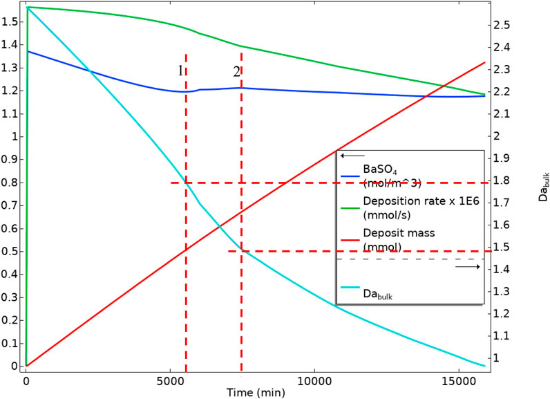
FIGURE 21. Average quantities of BaSO_4(aq) in bulk, Deposition rate on the surface, Deposit mass, and Bulk Damköhler number in Model 1 in a deforming geometry.

Figure 22 shows the bulk Damköhler number versus the available area inside the tube. As the deposition is occurring, the available area for the surface reaction (deposition) decreases. This reduction in the surface area and the shorter residence time for the production of the BaSO_4(aq) will reduce the surface reaction rate in the system.

FIGURE 22

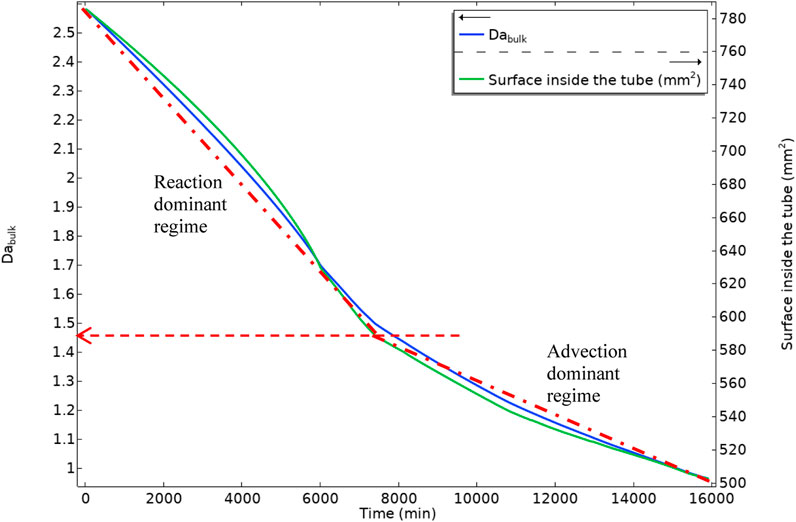
FIGURE 22. Bulk Damköhler number and the tube inside surface area versus time, dashed-dot lines are showing two different slopes in bulk Damköhler number.

Figure 23 shows the actual deformed geometry along the system with time. It is observable that the deposition takes place at the initial part of the tube. As this deposition near the inlet happens, the local residence time reduces, and the BaSO_4(aq) plume moves further down the tube. The BaSO_4(aq) concentration is a driving force for the deposition, so the more it moves down the line, the more deposition occurs closer to the outlet of the tube. At later times, the available surface area for deposition at the tube inlet also contributes to the reduction in deposition rate close to the tube inlet.

FIGURE 23

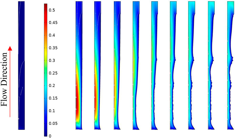
FIGURE 23. Tube deformed geometry at 0, 1666.6, 3333.2, 4999.8, 6666.4, 8333, 9999.6, 11666.2, 13332.8, and 14999.4 min respectively from left to right. The surface colour shows the concentration of BaSO_4(aq).

Figure 24 shows the system dynamics in terms of local residence time and local velocity change with deforming geometry. It is observable from Figure 24A that the residence time in the section near the inlet drops with a sharper slope in comparison with the section near the outlet. The residence time in the section near the inlet (blue curve in Figure 24) has two slopes. As discussed above, at lower flow rates, the deposition mainly occurs near the inlet of the cell. That deposition changes the geometry leading to a lower residence time that reduces the deposition rate. This reduction in deposition rate, in turn, reduces the deformation rate of the system and thus a smaller change in local residence time. The local residence time near the outlet section (green curve in Figure 24) also has a sharper slope when the local residence time near the beginning has dropped significantly. This change in slope is because the BaSO_4(aq) plume has moved further down the tube with a subsequent deposition.

FIGURE 24

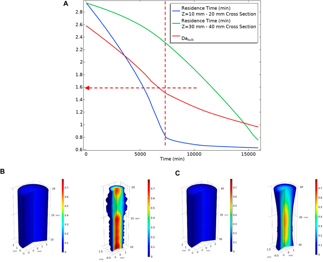
FIGURE 24. (A) Local Residence Time at two different sections of the tube (B) A section of the tube from Z = 10 mm to Z = 20 mm Left: before the deposition occurs, Right: After deposition changed geometry at t = 15,000 min. The surface colour shows velocity. (C) A section of the tube from Z = 30 mm to Z = 40 mm Left: before the deposition occurs, Right: After deposition changed geometry at t = 15,000 min. The surface colour shows velocity.

Summary and conclusion

In this work, a detailed study is presented of the dynamic behaviour of barite (BaSO₄) deposition by using a Computational Fluid Dynamics approach coupled with a kinetic model of barium sulphate formation and surface deposition. The full Navier-Stokes equations are solved in a flow channel coupled with a transport equation to accurately capture the effect of residence time. Our results give us a much improved understanding of the interplay between different aspects of both the chemical kinetic and fluid flow physics of the process. Accurately predicting the deposition of scale in a laminar flow system requires understanding the important characteristic length known as the diffusion penetration length (δ); this quantity represents the mass transfer region where solutes are transported from the bulk fluid to the solid surface. To calculate this length, resolving the flow field using high-resolution Navier-Stokes equations is central to our understanding of the depositional process. It is important to distinguish the diffusion penetration length from the hydraulic boundary layer, which should not be confused despite their interrelatedness. Furthermore, in simulating turbulent flow, such as with the Reynolds Averaged Navier Stokes equations, it becomes crucial to address the near-wall effect through a range of equations, as turbulence affects the effective diffusivity of the system. An accurate understanding of the hydrodynamic layer is vital in calculating the local residence time and diffusion time and can, therefore, help predict the location of the deposited scale. Since the velocity is zero near the wall, understanding of the hydrodynamic layer would provide insight in calculating the local residence time and diffusion time. Thus, it can help to predict the location of the deposited scale.

Our understanding was built up by taking a range of approaches to the modelling of this reactive-transport system by calculating the effect on the barite deposition behaviour by exploring the following scenarios:

1. Constant flow cases.

2. A ramp-up flow scan calculations.

3. Simulating cases allowing for the deforming geometry due to barite deposition.

We have shown the effect of parameters that change the Damköhler number (Da) on the reaction in the fluid bulk and on the surface. This provides a good understanding of how a flowing system can change the balance of deposition mechanisms from reaction dominated to advection dominated or vice-versa.

We have demonstrated that a system may go from a reaction dominated deposition regime into an advection dominated regime as the deposition is taking place. Thus, the deformation of the geometry and changes in the local residence time should be taken into account in calculations performed in industrial cases.

Two different but related models of the deposition mechanisms are presented here, denoted as Model 1 and Model 2. The variability in the surface deposition rate demonstrated that the surface effect is important in choosing either of these models. In rougher surfaces, where deposition constant would be higher, Model 2 is closer to reality, whereas in smoother surfaces, Model 1 may captures the deposition mechanism quite adequately.

The simulation framework is qualitatively supported and illustrated by results from a set of barite deposition flow laboratory experiments work which show the evolution of the deposition regime from a reaction dominated mechanism into an advection dominated one.

As a result of this mechanistic study, we show that at lower flowrates, the deposition takes place near the inlet vicinity of the tube, and as the flow increases, the deposition location moves towards the outlet vicinity of the tube. However, within the same case, if there is a rough surface within the pipe or duct, the deposition may happen closer to the inlet of the system as the reaction mechanism tends to be more by direct ion deposition as opposed to deposition through an intermediate phase (the nanocrystalline BaSO_{4 (aq)}).

Data availability statement

The original contributions presented in the study are included in the article/Supplementary Material, further inquiries can be directed to the corresponding author.

Author contributions

HR, as the PhD student, carried out much of the work supervised by KS and EM (his PhD supervisors). KS devised the details of the barium sulphate kinetic model and wrote much of the paper. EM contributed to the developing ideas in the work and made many technical suggestions. EM also edited the paper and made many suggestions on the presentation of the work. All authors contributed to the article and approved the submitted version.

Funding

HR’s PhD studentship was funded by the Danish Hydrocarbon Research and Technology Centre (DHRTC) under contract CTR.2.D.04_CA_126. Energi Simulation are thanked for supporting the Chair in CCUS and Reactive Flow Simulation held by EM.

Conflict of interest

The authors declare that the research was conducted in the absence of any commercial or financial relationships that could be construed as a potential conflict of interest.

Publisher’s note

All claims expressed in this article are solely those of the authors and do not necessarily represent those of their affiliated organizations, or those of the publisher, the editors and the reviewers. Any product that may be evaluated in this article, or claim that may be made by its manufacturer, is not guaranteed or endorsed by the publisher.

Supplementary material

The Supplementary Material for this article can be found online at: https://www.frontiersin.org/articles/10.3389/fmats.2023.1198176/full#supplementary-material

References

Anabaraonye, B. U., Bentzon, J. R., Khaliqdad, I., Feilberg, K. L., Andersen, S. I., and Walther, J. H. (2021). The influence of turbulent transport in reactive processes: A combined numerical and experimental investigation in a taylor-Couette reactor. Chem. Eng. J. 421, 129591. doi:10.1016/j.cej.2021.129591

CrossRef Full Text | Google Scholar

Bhandari, N., Kan, A., Dai, Z., Zhang, F., Yan, F., Ruan, G., et al. (2016). “Effect of hydrodynamic pressure on mineral precipitation kinetics and scaling risk at HPHT,” in SPE International Oilfield Scale Conference and Exhibition, Aberdeen, UK., May 11-12, 2016.

CrossRef Full Text | Google Scholar

Boak, L. S., and Sorbie, K. S. (2006). “The kinetics of sulphate deposition in seeded and unseeded tests,” in SPE International Oilfield Scale Symposium, Aberdeen, UK, May 30-June 1, 2006.

Google Scholar

Boak, L. S., Sorbie, K. S., and Ziadi, C. (2007). “Barite deposition kinetic studies: Flow cell experimental results and modelling,” in 18th International Oil Field Chemistry Symposium, Geilo, Norway, March 25-28, 2007.

Google Scholar

Borgia, A., Pruess, K., Kneafsey, T. J., Oldenburg, C. M., and Pan, L. (2012). Numerical simulation of salt precipitation in the fractures of a CO2-enhanced geothermal system. Geothermics 44, 13–22. doi:10.1016/j.geothermics.2012.06.002

CrossRef Full Text | Google Scholar

Boyd, V., Yoon, H., Zhang, C., Oostrom, M., Hess, N., Fouke, B., et al. (2014). Influence of Mg2+ on CaCO3 precipitation during subsurface reactive transport in a homogeneous silicon-etched pore network. Geochimica Cosmochimica Acta 135, 321–335. doi:10.1016/j.gca.2014.03.018

CrossRef Full Text | Google Scholar

Bracco, J. N., Lee, S. S., Stubbs, J. E., Eng, P. J., Heberling, F., Fenter, P., et al. (2017). Hydration structure of the barite (001)–water interface: Comparison of X-ray reflectivity with molecular dynamics simulations. J. Phys. Chem. C 121 (22), 12236–12248. doi:10.1021/acs.jpcc.7b02943

CrossRef Full Text | Google Scholar

Canic, T., Baur, S., Bergfeldt, T., and Kuhn, D. (2015). “Influences on the barite precipitation from geothermal brines,” in Proceedings World Geothermal Congress, Melbourne, Australia, April 19-25, 2015.

Google Scholar

Chakraborty, D., and Patey, G. N. (2013). How crystals nucleate and grow in aqueous NaCl solution. J. Phys. Chem. Lett. 4 (4), 573–578. doi:10.1021/jz302065w

PubMed Abstract | CrossRef Full Text | Google Scholar

Dai, C., Stack, A. G., Koishi, A., Fernandez-Martinez, A., Lee, S. S., and Hu, Y. (2016). Heterogeneous nucleation and growth of barium sulfate at organic-water interfaces: Interplay between surface hydrophobicity and Ba(2+) adsorption. Langmuir 32 (21), 5277–5284. doi:10.1021/acs.langmuir.6b01036

PubMed Abstract | CrossRef Full Text | Google Scholar

De La Pierre, M., Raiteri, P., Stack, A. G., and Gale, J. D. (2017). Uncovering the atomistic mechanism for calcite step growth. Angew. Chem. Int. Ed. Engl. 56 (29), 8464–8467. doi:10.1002/anie.201701701

PubMed Abstract | CrossRef Full Text | Google Scholar

Emmanuel, S., Ague, J. J., and Walderhaug, O. (2010). Interfacial energy effects and the evolution of pore size distributions during quartz precipitation in sandstone. Geochimica Cosmochimica Acta 74 (12), 3539–3552. doi:10.1016/j.gca.2010.03.019

CrossRef Full Text | Google Scholar

Fogler, H. S. (2010). Essentials of chemical reaction engineering: Essenti chemica reactio engi. London, UK: Pearson Education.

Google Scholar

Fu, Y., van Berk, W., and Schulz, H.-M. (2012). Hydrogeochemical modelling of fluid–rock interactions triggered by seawater injection into oil reservoirs: Case study Miller field (UK North Sea). Appl. Geochem. 27 (6), 1266–1277. doi:10.1016/j.apgeochem.2012.03.002

CrossRef Full Text | Google Scholar

Gebauer, D., Kellermeier, M., Gale, J. D., Bergstrom, L., and Colfen, H. (2014). Pre-nucleation clusters as solute precursors in crystallisation. Chem. Soc. Rev. 43 (7), 2348–2371. doi:10.1039/c3cs60451a

PubMed Abstract | CrossRef Full Text | Google Scholar

Godinho, J. R. A., and Stack, A. G. (2015). Growth kinetics and morphology of barite crystals derived from face-specific growth rates. Cryst. Growth and Des. 15 (5), 2064–2071. doi:10.1021/cg501507p

CrossRef Full Text | Google Scholar

Godinho, J. R., Gerke, K. M., Stack, A. G., and Lee, P. D. (2016). The dynamic nature of crystal growth in pores. Sci. Rep. 6, 33086. doi:10.1038/srep33086

PubMed Abstract | CrossRef Full Text | Google Scholar

Graham, A., Boak, L., Neville, A., and Sorbie, K. (2005). “How minimum inhibitor concentration (MIC) and sub-MIC concentrations affect bulk precipitation and surface scaling rates,” in Proceedings of the International Symposium on Oilfield Chemistry, Houston, TX, USA, February 2-4, 2005, 2–4.

CrossRef Full Text | Google Scholar

Hasson, D., Shemer, H., and Sher, A. (2011). State of the art of friendly “green” scale control inhibitors: A review article. Industrial Eng. Chem. Res. 50 (12), 7601–7607. doi:10.1021/ie200370v

CrossRef Full Text | Google Scholar

Kügler, R. T., Beißert, K., and Kind, M. (2016). On heterogeneous nucleation during the precipitation of barium sulfate. Chem. Eng. Res. Des. 114, 30–38. doi:10.1016/j.cherd.2016.07.024

CrossRef Full Text | Google Scholar

Løge, I. A., Bentzon, J. R., Klingaa, C. G., Walther, J. H., Anabaraonye, B. U., and Fosbøl, P. L. (2022). Scale attachment and detachment: The role of hydrodynamics and surface morphology. Chem. Eng. J. 430, 132583. doi:10.1016/j.cej.2021.132583

CrossRef Full Text | Google Scholar

Mavredaki, E., Neville, A., and Sorbie, K. (2011). Assessment of barium sulphate formation and inhibition at surfaces with synchrotron X-ray diffraction (SXRD). Appl. Surf. Sci. 257 (9), 4264–4271. doi:10.1016/j.apsusc.2010.12.034

CrossRef Full Text | Google Scholar

May, R., Akbariyeh, S., and Li, Y. (2012). Pore-scale investigation of nanoparticle transport in saturated porous media using laser scanning cytometry. Environ. Sci. Technol. 46 (18), 9980–9986. doi:10.1021/es301749s

PubMed Abstract | CrossRef Full Text | Google Scholar

Meldrum, F. C., and O'Shaughnessy, C. (2020). Crystallization in confinement. Adv. Mater 32 (31), e2001068. doi:10.1002/adma.202001068

PubMed Abstract | CrossRef Full Text | Google Scholar

Molins, S., Trebotich, D., Yang, L., Ajo-Franklin, J. B., Ligocki, T. J., Shen, C., et al. (2014). Pore-scale controls on calcite dissolution rates from flow-through laboratory and numerical experiments. Environ. Sci. Technol. 48 (13), 7453–7460. doi:10.1021/es5013438

PubMed Abstract | CrossRef Full Text | Google Scholar

Poonoosamy, J., Kosakowski, G., Van Loon, L. R., and Mader, U. (2015). Dissolution-precipitation processes in tank experiments for testing numerical models for reactive transport calculations: Experiments and modelling. J. Contam. Hydrol. 177-178, 1–17. doi:10.1016/j.jconhyd.2015.02.007

PubMed Abstract | CrossRef Full Text | Google Scholar

Prasianakis, N. I., Curti, E., Kosakowski, G., Poonoosamy, J., and Churakov, S. V. (2017). Deciphering pore-level precipitation mechanisms. Sci. Rep. 7 (1), 13765. doi:10.1038/s41598-017-14142-0

PubMed Abstract | CrossRef Full Text | Google Scholar

Putnis, A. (2015). Transient porosity resulting from fluid–mineral interaction and its consequences. Rev. Mineralogy Geochem. 80 (1), 1–23. doi:10.2138/rmg.2015.80.01

CrossRef Full Text | Google Scholar

Ruiz-Agudo, C., Ruiz-Agudo, E., Putnis, C. V., and Putnis, A. (2015). Mechanistic principles of barite formation: From nanoparticles to micron-sized crystals. Cryst. Growth and Des. 15 (8), 3724–3733. doi:10.1021/acs.cgd.5b00315

CrossRef Full Text | Google Scholar

Shields, R., Bourne, H., Vazquez, O., Sorbie, K., and Singleton, M. (2010). “Dynamic scaling evaluation in gravel packs using low-sulphate seawater,” in SPE International Symposium and Exhibition on Formation Damage Control, Lafayette, Louisiana, February 10-12, 2010.

CrossRef Full Text | Google Scholar

Stack, A. G. (2014). Next generation models of carbonate mineral growth and dissolution. Greenh. Gases Sci. Technol. 4 (3), 278–288. doi:10.1002/ghg.1400

CrossRef Full Text | Google Scholar

Stack, A. G. (2015). Precipitation in pores: A geochemical frontier. Rev. Mineralogy Geochem. 80 (1), 165–190. doi:10.2138/rmg.2015.80.05

CrossRef Full Text | Google Scholar

Steefel, C. I., Appelo, C. A. J., Arora, B., Jacques, D., Kalbacher, T., Kolditz, O., et al. (2014). Reactive transport codes for subsurface environmental simulation. Comput. Geosci. 19 (3), 445–478. doi:10.1007/s10596-014-9443-x

CrossRef Full Text | Google Scholar

Wat, R., Sorbie, K., Todd, A., Ping, C., and Ping, J. (1992). “Kinetics of BaSO4 crystal growth and effect in formation damage,” in SPE Formation Damage Control Symposium, Lafayette, Louisiana, February 26, 1992.

CrossRef Full Text | Google Scholar

Weber, J., Bracco, J. N., Poplawsky, J. D., Ievlev, A. V., More, K. L., Lorenz, M., et al. (2018). Unraveling the effects of strontium incorporation on barite growth—in situ and ex situ observations using multiscale chemical imaging. Cryst. Growth and Des. 18 (9), 5521–5533. doi:10.1021/acs.cgd.8b00839

CrossRef Full Text | Google Scholar

Weber, J., Bracco, J. N., Yuan, K., Starchenko, V., and Stack, A. G. (2021a). Studies of mineral nucleation and growth across multiple scales: Review of the current state of research using the example of barite (BaSO4). ACS Earth Space Chem. 5, 3338–3361. doi:10.1021/acsearthspacechem.1c00055

CrossRef Full Text | Google Scholar

Weber, J., Cheshire, M. C., Bleuel, M., Mildner, D., Chang, Y.-J., Ievlev, A., et al. (2021b). Influence of microstructure on replacement and porosity generation during experimental dolomitization of limestones. Geochimica Cosmochimica Acta 303, 137–158. doi:10.1016/j.gca.2021.03.029

CrossRef Full Text | Google Scholar

Yan, F., Dai, Z., Ruan, G., Alsaiari, H., Bhandari, N., Zhang, F., et al. (2017). Barite scale formation and inhibition in laminar and turbulent flow: A rotating cylinder approach. J. Petroleum Sci. Eng. 149, 183–192. doi:10.1016/j.petrol.2016.10.030

CrossRef Full Text | Google Scholar

Yang, F., Stack, A. G., and Starchenko, V. (2021). Micro-continuum approach for mineral precipitation. Sci. Rep. 11 (1), 3495. doi:10.1038/s41598-021-82807-y

PubMed Abstract | CrossRef Full Text | Google Scholar

Yi-Tsung Lu, A., Kan, A. T., and Tomson, M. B. (2021). Nucleation and crystallization kinetics of barium sulfate in the hydrodynamic boundary layer: An explanation of mineral deposition. Cryst. Growth and Des. 21 (3), 1443–1450. doi:10.1021/acs.cgd.0c01027

CrossRef Full Text | Google Scholar

Yoon, H., Chojnicki, K. N., and Martinez, M. J. (2019). Pore-scale analysis of calcium carbonate precipitation and dissolution kinetics in a microfluidic device. Environ. Sci. Technol. 53 (24), 14233–14242. doi:10.1021/acs.est.9b01634

PubMed Abstract | CrossRef Full Text | Google Scholar

Yoon, H., Valocchi, A. J., Werth, C. J., and Dewers, T. (2012). Pore-scale simulation of mixing-induced calcium carbonate precipitation and dissolution in a microfluidic pore network. Water Resour. Res. 48 (2). doi:10.1029/2011wr011192

CrossRef Full Text | Google Scholar

Zhang, J. W., and Nancollas, G. H. (2018). “Chapter 9. Mechanisms of growth and dissolution of sparingly soluble salts,” in Mineral-water interface geochemistry. Editors F. H. Michael, and F. W. Art (Berlin, Germany: De Gruyter), 365–396.

Google Scholar

Zhen-Wu, B. Y., Dideriksen, K., Olsson, J., Raahauge, P. J., Stipp, S. L. S., and Oelkers, E. H. (2016). Experimental determination of barite dissolution and precipitation rates as a function of temperature and aqueous fluid composition. Geochimica Cosmochimica Acta 194, 193–210. doi:10.1016/j.gca.2016.08.041

CrossRef Full Text | Google Scholar