Numerical simulation of inductive heating in thermoplastic unidirectional cross-ply laminates

Thermoplastic Composites can be re-melted allowing them to be joined via welding. This is an attractive alternative to conventional methods that are used to join thermoset composite parts such as mechanical fastening and adhesive bonding. In this work the inductive heating of uni-directional (UD) plies of thermoplastic carbon fiber reinforced polymer (CFRP) laminates is investigated. The focus is on developing a numerical electromagnetic and thermal simulation model that captures the main processes involved in eddy current generation and heat generation, in particular in the interface areas of the UD plies. A measurement technique has been developed to obtain the electric properties of the ply material. Furthermore, to support the modelling of both the induction heating equipment and work piece a field measurement of the magnetic field surrounding the coil and work piece has been developed. Inductive heating experiments were carried out on several thick composite laminate plates with different ply lay-ups to compare and validate the electro-magnetic-thermal simulation model. The measured surface temperatures were compared with the results from the simulation model. The results of this work can be used to support the design of UD-ply laminates to improve their ability to be welded via inductive heating. In addition, the results of this work can be used to assist in pre-determining induction welding equipment settings and heating times.

1 Introduction

In the Large Passenger Aircraft Platform 2 of the European R&D program Clean Sky 2, a Multifunctional Fuselage Demonstrator (MFFD) for single aisle aircraft is developed that serves as a platform for examining the full potential of Thermoplastic (TP) composites. This TP composite MFFD shall demonstrate the benefits of integrating various functionalities and help future European airliner production to become faster, greener, and more competitive. Significant weight reduction and thus environmental improvements of aircraft are expected as a result of innovative manufacturing, assembly, and installation processes. These innovations in turn will drive down costs and improve product competitiveness to European aeronautics. The TP composite MFFD consists of an assembly of multi-functional building blocks for the next-generation fuselage and cabin. Development of advanced joining technologies and effective use of materials is necessary to enable a competitive assembly.

One example of such advanced joining techniques is induction welding (Christopoulos, 1990). TP composites can be re-melted allowing them to be joined via welding (Mitschang, et al., 2000). At present, the inductive heating of woven fabric composites is well documented and understood (Yousefpour, et al., 2004). Several heating mechanisms take place in the induction heating of TP carbon fiber reinforced polymer (CFRP). The extent in which each mechanism contributes to the heating process, depends on the material that is heated and the process parameters that are applied. However, a Uni-Directional (UD) CFRP material is more difficult to heat than a weave CFRP material. According to literature (Ahmed, et al., 2006) this could be due to the absence of a current returning path that is naturally embedded in the weave.

The objective of this work is to develop 3D electromagnetic simulation models coupled to 3D thermal simulation models that can provide insight into the inductive heating of UD plies of thermoplastic CFRP laminates. Investigations include the influence of the UD plies and the ply interfaces on the eddy current generation and heat generation inside a UD CFRP laminate when placed inside an electromagnetic field that is induced by a coil. First, basic steps for modelling eddy current generation in a CFRP laminate are introduced. Second, a numerical simulation model based on electromagnetic Finite Element (FE) analysis is introduced. This model is extended with an updated version of a cross-ply interface model (de Wit, et al., 2021) previously developed by the authors. The updated interface model is constructed analogous to a surface implementation (Cheng, et al., 2021) but is extended to a volumetric implementation in this work. Third, electrical conductivity measurements were performed to determine necessary material parameters for the numerical modelling. Furthermore, magnetic field measurements near the induction welding equipment were performed to obtain confidence in the electromagnetic modelling of the setup. Fourth, inductive heating measurements were carried out and compared with the results obtained from the simulation models. Finally, the main conclusions and steps for further research are presented.

2 Electromagnetic modelling

For induction welding (IW) of TP CFRP, the electromagnetic properties of the plies and the laminate layup are of key importance for the electromagnetic behavior of the electromagnetic eddy currents that emerge in the CFRP composite laminate. Apart from the magnetic permeability and magnetic permittivity, the electric conductivity of the material is a key determinant for the eddy current density distribution in the laminate. Although these properties depend on temperature and frequency, in the current study these properties are kept constant.

2.1 Cross-ply laminates and ply interfaces

Induction heating is accomplished via Eddy currents that are generated in the carbon fibers through the magnetic field from a coil. For Eddy currents to occur, closed loops of electrically conductive paths are necessary. Hence, current flowing along the fibers has to be able to return back along another set of fibers. If there is sufficient galvanic connection a conductive loop is created. Typically, in woven fabrics this is easily established as the fibers make contact in the weave. For UD material this contact is not evident.

If insufficient contact between fibers is present such as in UD material, the only way for current to flow in a closed loop is via capacitive coupling through the polymer matrix. For most polymers this can only occur at very high frequencies (several MHz). In such cases additional heat is generated via dielectric losses in the polymer. Since equipment that can operate at frequencies of several MHz is not applicable in our setup this form of heating is not considered.

For UD material another option remains to create electrical closed loops. When UD material is stacked at different angles with respect to each other cross-ply interfaces are formed that close the current loop (O’Shaughnessey et al., 2016). This is shown in Figure 1.

FIGURE 1

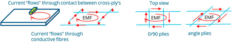
FIGURE 1. Cross-plies form a closed loop such that current can ‘flow’ through the plies. EMF stands for electromagnetic field.

At these interfaces contact resistance forms an additional heating mechanism in addition to the Joule Heating coming from the fiber resistance (Kim et al., 2000). These cross-fiber contacts result in a more isotropic in-plane conductivity and increased out-of-plane conductivity in this interface layer. To incorporate this important effect, the augmented electric conductivity properties in the cross-ply interfaces must be included in the FE model.

2.2 Cross-ply interface definition

In this work we develop an approach for solid FE modelling of electromagnetic eddy currents in cross-ply laminates including their cross-ply interfaces. To develop the interface concept, we consider a small two-ply laminate sample with arbitrary thickness (t), width (w) and length (L). Furthermore, two interface cases are considered. The first consists of a [0,0] UD laminate and the second of a [0,90] cross-ply laminate. The x-axis is taken along the two-ply laminate length direction, y-axis is taken along the two-ply width direction and z-axis along the thickness of the two-ply thickness direction. Each ply has a total thickness of t_ply. The cross-section is sketched in Figure 2.

FIGURE 2

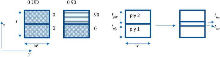
FIGURE 2. Front view of the small 2-ply laminate sample. A UD [0,0]and a cross-ply [0,90] laminate are shown. The 0 fibers are oriented in x-direction. Each ply has a total thickness t_ply. The cross-ply interface layer of arbitrary finite thickness t_int per ply is considered in between the ply. Hence, the interface layer thickness is 2*t_int.

In the region around the interface between the plies, a cross-ply interface layer of arbitrary but finite thickness t_int per ply is introduced, see Figure 2. This interface layer is considered to have the augmented anisotropic electric conductivity properties. Furthermore, these properties are taken homogeneous throughout the whole interface. The in-plane conductivities in the interface layer are assumed to result from the combination or mixture of the conductivities of the two plies. The out-of-plane conductivity in the interface layer is taken equal to the out-of-plane conductivity (or resistivity) of the considered cross-ply.

2.3 Electric resistances of plies and interface

The anisotropic resistance tensor for each of the two plies (ply 1 and ply 2) in the small laminate sample (recall Figure 2) contains the resistances of each of the two plies in the three directions x,y,z, see Figure 3.

FIGURE 3

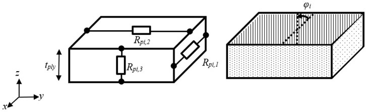
FIGURE 3. Illustration of the anisotropic resistances (left) and fiber orientation expressed by ply angle ${\mathit{\phi }}_{\mathit{i}}$ (right) for a single ply in the small laminate sample.

Hence, the resistances are written as:

${\mathit{R}}_{\mathit{p}\mathit{i}}=\left[{\mathit{R}}_{\mathit{p}\mathit{i},\mathbf{1}}^{{\mathit{\phi }}_{\mathit{i}}},{\mathit{R}}_{\mathit{p}\mathit{i},\mathbf{2}}^{{\mathit{\phi }}_{\mathit{i}}},{\mathit{R}}_{\mathit{p}\mathit{i},\mathbf{3}}^{{\mathit{\phi }}_{\mathit{i}}}\right],\mathit{i}=\mathbf{1,2}(1)$

In Eq. 1, i is de ply index and each ply can have arbitrary ply orientation, expressed by a ply angle ${\phi }_i$. The resistances of a ply in the small laminate sample at an arbitrary ply angle ${\phi }_i$ can be determined by assuming a linear relation between the resistance in fibre direction ($R_{11}$) and the resistance in transverse direction ($R_{22}$) of a single ply, see (Cheng, et al., 2021). In this work however, this relation is considered non-linear:

${{\mathit{R}}_{\mathit{p}\mathit{i},\mathbf{1}}}^{{\mathit{\phi }}_{\mathit{i}}}={\mathit{\alpha }\mathit{R}}_{\mathbf{11}}+{\mathit{\beta }\mathit{R}}_{\mathbf{22}},{{\mathit{R}}_{\mathit{p}\mathit{i},\mathbf{2}}}^{{\mathit{\phi }}_{\mathit{i}}}={\mathit{\beta }\mathit{R}}_{\mathbf{11}}+{\mathit{\alpha }\mathit{R}}_{\mathbf{22}},\mathit{i}=\mathbf{1,2}(2)$

$\mathit{\alpha }={\left(\mathbf{cos}{\mathit{\phi }}_{\mathit{i}}\right)}^{\mathbf{2}},\mathit{\beta }={\left(\mathbf{sin}{\mathit{\phi }}_{\mathit{i}}\right)}^{\mathbf{2}}(3)$

Since the interface layer has finite thickness (recall Figure 2 right), the total resistance in each direction x,y,z of the small two-ply laminate sample must be equal to the total resistance of the sample without the interface layer (Figure 2 left). This yields that the resistance of the whole interface is equal to the combined resistance of its components. Hence, the lower half of the interface that contains the ply 1 properties and the upper half of the interface that contains the ply 2 properties.

Consequently, the in-plane resistances of the interface, i.e., in x,y directions, are composed of the parallel resistances of the interface components:

${\mathit{R}}_{\mathit{i},\mathit{j}}=\frac{{\mathit{R}}_{\mathit{i}\mathbf{1},\mathit{j}}{\mathit{R}}_{\mathit{i}\mathbf{2},\mathit{j}}}{{\mathit{R}}_{\mathit{i}\mathbf{1},\mathit{j}}{+\mathit{R}}_{\mathit{i}\mathbf{2},\mathit{j}}},\mathbf{j}=\mathbf{1,2}(4)$

Here $R_{i,j}$ is the resistance of the whole interface in direction j, and $R_{i1,j}$ is the lower interface component resistance and $R_{i2,j}$ is the upper interface component resistance, in direction j, with j = 1,2,3 that refers to the x,y,z directions.

The out-of-plane resistance of the interface, i.e.,.in z direction, is composed of the serial interface component resistances, and an additional ply-contact resistance. In (Xu, et al., 2018) this ply-contact resistivity (denoted by ${\rho }_c$ ) is determined experimentally for two-ply laminate samples.

2.4 Numerical simulation model electromagnetic field

The electromagnetic simulations are carried out in the FE package Abaqus (Simulia, 2023). In Abaqus a time-harmonic eddy current analysis procedure is used, which assumes that a tim-harmonic excitation such as an alternating current in the coil results in a time-harmonic electromagnetic response of electric and magnetic field with the same frequency everywhere in the domain.

The equations involved solving the inductive heating of thermoplastic material are presented in generic terms following the outline in (Chen, 2016). The electric and magnetic fields are governed by Maxwell’s equations

$\nabla \bullet \mathit{E}={\mathit{\rho }}_{\mathit{E}};\nabla \bullet \mathit{B}=\mathbf{0};\nabla \times \mathit{E}=-\frac{\partial \mathit{B}}{\partial \mathit{\tau }};\nabla \times \mathit{H}=\mathit{J}+\frac{\partial \mathit{D}}{\partial \mathit{\tau }}(5)$

Where ${\rho }_E$ the electric charge density, $\mathit{E}$ the electric field, $\mathit{B}$ the magnetic induction, $\mathit{D}$ the electric flux density, $\mathit{J}$ the electric current density, $\mathit{H}$ the magnetic field and $\tau$ corresponds to time. The following constitutive relations are substituted:

$\mathit{D}={\mathit{ϵ}}_{\mathbf{0}}{\mathit{ϵ}}_{\mathit{r}}\mathit{E};\mathit{B}={\mathit{\mu }}_{\mathbf{0}}{\mathit{\mu }}_{\mathit{r}}\mathit{H};\mathit{J}=\mathit{\sigma }\bullet \mathit{E}(6)$

Where ${ϵ}_0$ absolute permittivity, ${ϵ}_r$ relative permittivity, ${\mu }_0$ absolute magnetic permeability, ${\mu }_{\mathit{r}}$ relative permeability and $\sigma$ the conductivity tensor.

The joule heating is computed via:

$\dot{\mathit{Q}}={\mathit{J}}^{\mathit{T}}\bullet {\mathit{\sigma }}^{=-\mathbf{1}}\bullet \mathit{J}(7)$

This joule heating is used to calculate the temperature distribution of the thermoplastic laminate by the heat equation:

$\mathit{\rho }{\mathit{c}}_{\mathit{p}}\frac{\partial \mathit{T}}{\partial \mathit{\tau }}-\nabla \bullet \left(\mathit{\lambda }=\nabla \mathit{T}\right)=\dot{\mathit{Q}}(8)$

Where $\rho$ is the density, $c_p$ the specific heat coefficient, $\mathit{\lambda }$ the thermal conductivity tensor.

In the case of eddy current analysis it is typical that large portions of the model consist of electrically non-conductive regions such as air. In such case the problem becomes ill-conditioned and Abaqus uses an iterative solution technique to prevent a negative impact on the computed electric and magnetic fields. In some cases this technique may not work and Abaqus advices to add artificial electrical conductivity to convert to a solution. It is recommended to set this artificial conductivity about five to eight orders of magnitude less than that of the conductors in the model. As will be shown in the next section, the electric conductivity in ply direction is an order of magnitude four higher than in the non-ply direction. Hence, it is difficult to add artificial conductance and not affect the computed results in out-of-ply directions in Abaqus.

2.4.1 Model geometry, load and boundary conditions

To capture 3D effects of the induction setup a 3D FEA model is constructed. The overall lay-out of the coil and laminate is shown in Figure 4. A top view of the lay-out showing the coil centered above the laminate is shown in Figure 4B.

FIGURE 4

FIGURE 4. (A) Overall lay-out of the coil and laminate. (B) Top view of the coil above the laminate.

The distance between coil and laminate is 14 [mm]. The coil cross section has an outer diameter of 6.35 [mm] and inner diameter of 4.35 [mm]. The overall dimensions of the coil and it’s position with respect to the laminate are shown in Figure 4, Figure 5.

FIGURE 5

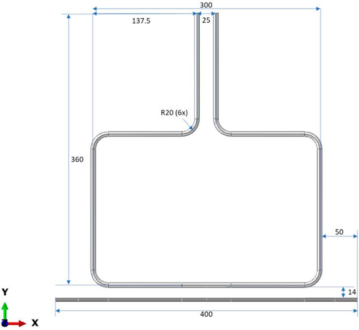
FIGURE 5. Dimensions of the coil in [mm] and position with respect to the laminate.

To reduce the computational effort and make use of symmetry conditions in the model only 1/4th of the model is included in the Abaqus model. Therefore, the symmetry plane parallel to the coil winding is modeled as a perfect magnetic conductor, see Figure 6.

FIGURE 6

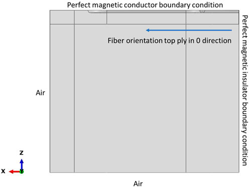
FIGURE 6. Model of 1/4th of the geometry. On the symmetry plane a perfect magnetic conductor boundary condition is applied. On the anti-symmetry plane a perfect magnetic insulator boundary condition is applied. At the two remaining edges of the plate a volume of air is modelled.

The boundary condition for the parallel symmetry plane is written as:

$\mathit{n}\times \mathit{H}=\mathbf{0}(9)$

This corresponds to the assumption that the current field is mirrored in this symmetry plane.

Perpendicular to the coil, the symmetry plane is modelled as a perfect magnetic insulator, see Figure 6. The boundary condition is written as:

$\mathit{n}\times \mathit{A}=\mathbf{0};\nabla \times \mathit{A}=\mathit{B}(10)$

Which corresponds to the assumption that the magnetic field normal to the symmetry plane equals zero and the current cannot have a tangential component.

Because the laminates considered in this work have a ply orientation of 0° or 90° these symmetry conditions can also be applied to the composite laminate. Furthermore, surrounding the coil and laminate a box of air is modelled with dimensions 400 × 400 × 500 mm. The external surfaces of this box of air are assumed magnetic insulators:

$\mathit{n}\times \mathit{H}=\mathbf{0}(11)$

For the thermal simulation model only the geometry of the thermoplastic plate was considered. Hence, the boundary conditions with respect to air were modelled via a film coefficient:

$-{\mathit{\lambda }}_{\mathit{n}}\frac{\partial \mathit{T}}{\partial \mathit{n}}=\mathit{h}\left({\mathit{T}}_{\mathit{s}\mathit{k}\mathit{i}\mathit{n}}-{\mathit{T}}_{\mathit{a}}\right)(12)$

Where $h$ is the so-called film coefficient and $T_a$ the ambient or in this case room temperature. ${\lambda }_n$ is the thermal conductivity along the unit normal on the surface n. The convective heating coefficients for each surface of the plate are computed using the approach outlined in (Moser, 2012). For completeness the computed coefficients are shown in Figure 7.

FIGURE 7

FIGURE 7. Convection coefficients used on the top and bottom surface of the plate and the external sides exposed to the surrounding air.

The one-quarter model consists of a composite laminate with dimensions 200 [mm]x200 [mm] and 36 plies. Each ply has a thickness of 0.138 [mm]. Hence, the laminate thickness equals 5 [mm]. The coil consists of a single rectangle of which one-quarter is modelled. The coil is assumed to have homogenous material properties. To prevent Abaqus to calculate eddy currents for the volume of the coil that are then subtracted from the applied current load a conductivity of 1 [S/m] is used. Furthermore, a current of 199.5 [A] is applied in circumferential direction of the coil at a frequency of 194 [kHz].

2.4.2 Material properties

The material properties that are used in the present model for the air, coil and laminate are listed in Table 1.

TABLE 1

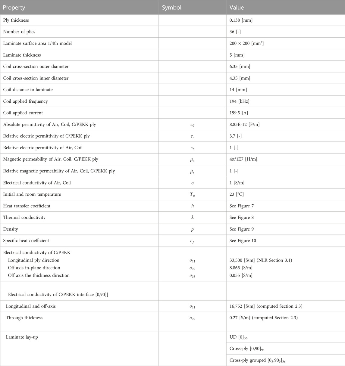
TABLE 1. Material properties for the air, coil and AS4D/PEKK taken from (Grouve, et al., 2020) unless indicated otherwise. Furthermore, dimensions and applied loading that were applied to the model.

FIGURE 8

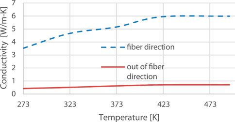
FIGURE 8. Thermal conductivity in fiber direction and out-of-fiber direction. These values were taken from (Yousefpour & Hojjati, 2011).

FIGURE 9

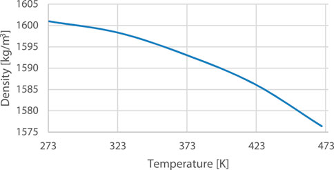
FIGURE 9. Density as a function of temperature for fibers, taken from (Yousefpour & Hojjati, 2011).

FIGURE 10

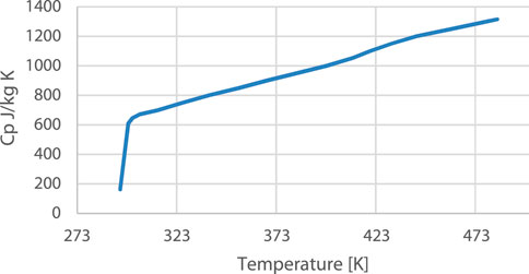
FIGURE 10. Specific heat for Toray Cetec TC1320 PEKK/AS4D. These properties were measured by NLR for several samples taken from the composite plates manufactured for this study. The average value of the measurements of the samples was taken.

The air surrounding the 1/4th coil and laminate is a box of 400 [mm] x 400 [mm] x 500 [mm]. Each ply is modeled separately and considered an homogenous anisotropic sheet. For meshing two elements are used in thickness direction for each ply, see Figure 11.

FIGURE 11

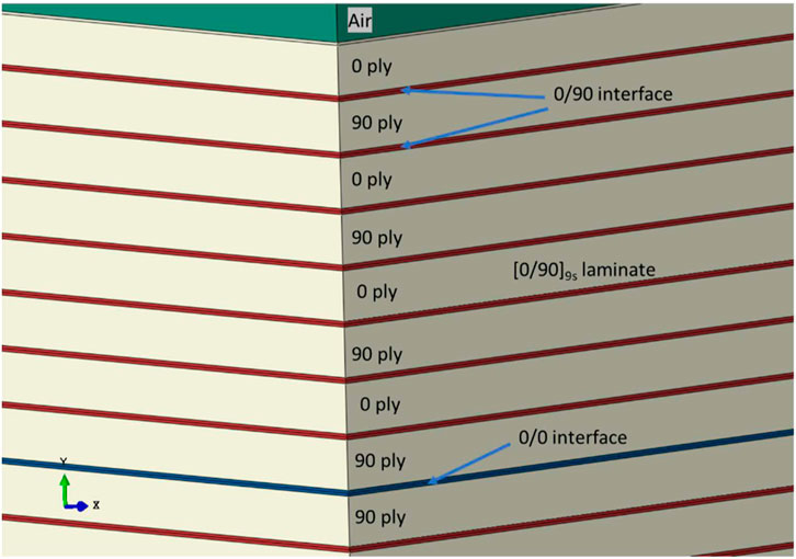
FIGURE 11. Modelling of plies and interfaces for a [0/90]_9s laminate. Each interface layer consists of a part of the top ply and a part of the bottom ply.

The whole model comprises 2.3 M EMC3D8 elements. A larger model did not fit on our current available computer hardware. Furthermore, in previous work (de Wit, et al., 2022) the mesh density that corresponds to this number of elements was found sufficient to capture both magnetic field and eddy current field. The interfaces between plies are taken as 10% of ply thickness. The interfaces consume 2 elements in thickness direction from each ply except for top and bottom ply that only assign one element to the interface.

3 Experiments to support the modelling

Although material data sheets include recognized standards for mechanical and thermal material properties, electrical properties are less common to be included. For UD material, an additional property involving the cross-ply electrical properties is application specific. Furthermore, to obtain confidence in the electromagnetic modelling field measurements were done on the induction heating setup to compare and validate the modelling approach.

3.1 UD ply electrical conductivity measurements

The anisotropic electrical conductivity of a single ply was characterized by measuring the resistance as outlined in (de Wit, et al., 2022). For completeness, the procedure is summarized here. A measurement in the longitudinal, transverse, and through-thickness direction was performed. For the experimental setup unconsolidated strips of UD tape material with a thickness of 0.21 [mm] were clamped between electrodes. For the resistance measurements in longitudinal direction (i.e., fibre direction) a 6.35 [mm] wide and 1,000 [mm] long specimen was used. For the resistance measurement in the transverse and through-thickness direction shorter specimens of 20 [mm] were used and the clamping devices were adjusted.

Five samples were used for each measurement and the Direct-Current (DC) resistance, as well as, the Alternating-Current (AC) impedance. The impedance was measured at several frequencies, that is: 50 [Hz], 25 [kHz], 50 [kHz], 75 [kHz], and 100 [kHz]. Each specimen was measured at two instances to exclude the influence of the test setup and clamping procedure. By using the specimen dimensions the resistance in Ohm was transformed to conductivity in [S/m].

The AC conductivity measurements were extrapolated to the frequency of the induction welding simulation (for this measurement, 384 [kHz]). The results of the longitudinal conductivity measurements were compared with values found in the literature for AS4D/PEKK. For two types of AS4D/PEKK Table 2 shows the electrical conductivity values compared to values obtained from literature.

TABLE 2

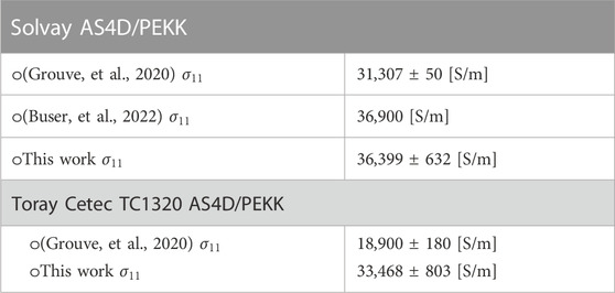
TABLE 2. Electrical conductivity properties found in literature and measured by NLR for AS4D/PEKK.

The values found are in close agreement with those obtained by (Grouve, et al., 2020) (Buser, et al., 2022). For the interface modelling conductivity properties have to be assigned to the interface elements as well. Such values can be determined via a similar measuring approach as outlined. Unfortunately, the measured electrical conductivity properties showed little consistency. It is the intention of the authors to repeat these measurements in future works.

3.2 Experimental magnetic field measurements

To obtain confidence in the numerical electromagnetic simulations, measurements were performed on the magnetic field surrounding the induction coil to compare the values with those obtained through simulation. The magnetic field was measured near the induction coil in the presence of air with no workpiece, with an aluminum workpiece, and a composite workpiece. In addition, the applied electrical load that is necessary for the FEA model was verified by measuring the current in the induction coil.

3.2.1 Experimental setup

Induction coils are designed with a specific application in mind. Therefore, many shapes and forms can be found for which different electromagnetic fields are constructed. In addition, the eddy currents that are generated in the workpiece are dependent on the coil shape and placement. Induction coils applied for studying inductive heating in composites, for instance (Grouve, et al., 2020), (Cheng, et al., 2021), usually have a different orientation and shape than the inductive heating equipment at NLR that was designed for welding long and slender structures. The inductive heating equipment corresponds to a setup developed by KVE Composites Group (Kok & Van Engelen). The generator consists of an Ambrell EASYHeat 83,100 LI that generates 10 [kW] at a frequency in the range of 150–400 [kHz]. The equipment is mounted on a KUKA KR 240 R2700 PRIME robot arm.

To capture the main characteristics of the electromagnetic field a long slender coil was used (dimensions listed in 2.4.1) that the authors expect to create a uniform field over a larger distance in the workpiece, see Figure 12A.

FIGURE 12

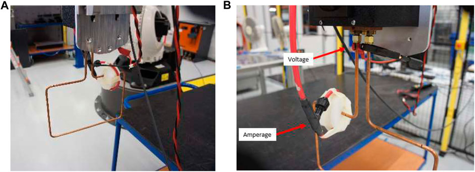
FIGURE 12. (A) Measurement of the Voltage and (B) Amperage applied to the coil.

An operator of the induction equipment has the option to choose the coil amperage. Based on this amperage, the induction machine applies an optimal frequency. It is unknown if the applied current matches the actual current in the coil. For electromagnetic simulations in Abaqus (Simulia, 2023) it is necessary to confirm the current in the induction coil. Therefore, the amperage and voltage in the coil were measured with a setup as shown in Figure 12B.

After the current measurements the coil was placed on a Styrofoam table that does not interfere with the magnetic field. For measuring the magnetic field a probe was used. The circular probe is made of a non-magnetic material (i.e., brass). The probe has an inner diameter of approximately 15 [mm] and a thickness of 5 [mm]. Using a known constant magnetic field the probe has been calibrated.

In order to measure the magnetic field close to the coil the magnetic field probe is positioned next to the coil as shown in Figures 13A, B.

FIGURE 13

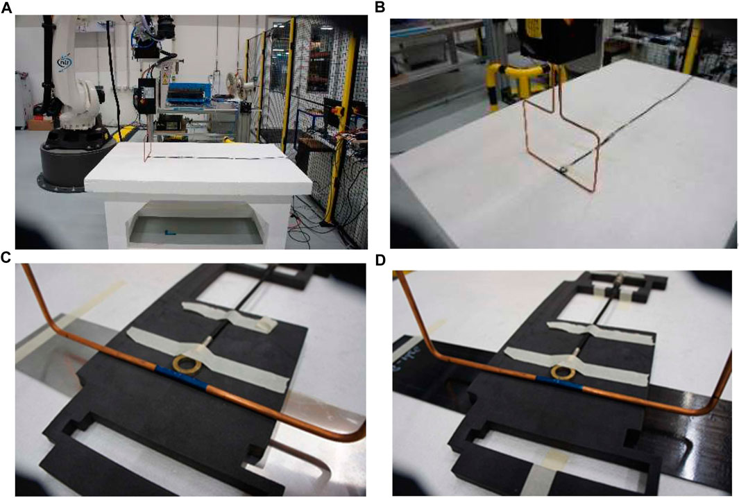
FIGURE 13. (A) The test setup for measuring the magnetic field around the induction coil. (B) Coil used to measure the magnetic field surrounding the induction coil and workpiece. Measurement of the magnetic field strength above the aluminum (C) and composite (D) plate.

The probe was connected to an oscilloscope for data acquisition in the frequency domain. The magnetic field that was captured inside the magnetic field probe was measured.

For the measurements with aluminium plate and composite plate a non-conductive material was placed in between the coil and workpiece to fix the positioning of the field probe, see Figures 13C, D. As a result, the coil and the probe have a constant spacing of 14 [mm] with the workpiece.

For the measurements in free air, with the aluminium plate, and with the composite plate the coil was moved horizontally in steps of 2 mm away from the probe. At each step the induction welding equipment was activated for 2 seconds to minimise heating of the workpiece. In this time, a measurement was taken and the frequency response from 100 [kHz] to 300 [kHz] was logged.

From basic electromagnetism theory, see Equation 13, it is known that magnetic flux density (B) decreases for increasing distance from the coil (r).

$\mathit{B}=\frac{{\mathit{\mu }}_{\mathbf{0}}\mathit{I}}{\mathbf{2}\mathit{\pi }\mathit{r}}(13)$

where ${\mu }_0$ is absolute magnetic permeability and $I$ is applied current.

Therefore, the magnetic field decreases within the probe inner surface. To compare the theoretical values, the probe measurements (and in the next section the simulation results) have to be recomputed to represent the average value over the probe inner area. It is assumed that the magnetic field is uniform in the length direction of the coil and the simulation and theoretical data is averaged using a circular integral corresponding to the probe inner diameter.

3.2.2 Measurement results and discussion

The voltage and amperage measurements were performed prior to the magnetic field measurement. Here the input amperage was increased from approximately 50 [A] to 200 [A]. The measured RMS values of the amperage and voltage are listed in Table 3.

TABLE 3

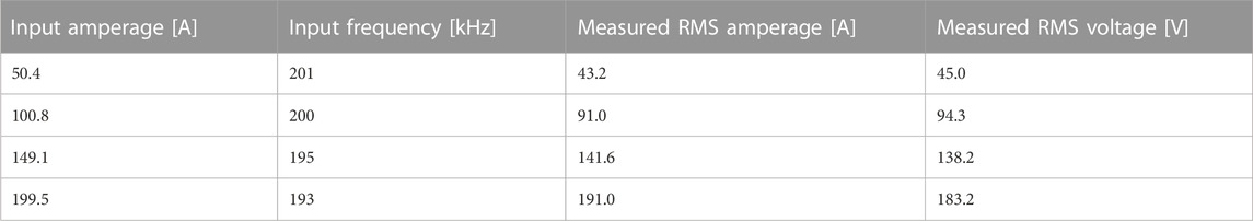
TABLE 3. RMS values of applied amperage and frequencies as measured.

From Table 3 it is observed that the optimal frequency set by the induction welding equipment decreases for increasing amperage. This is because at higher amperages a lower frequency is required to obtain the same induction power. The measured RMS amperage is slightly lower compared to the input amperage. From the detailed time response of the amperage signal it is observed that variations in time could be the cause of these differences.

For the magnetic B-field measurements an input amperage of 199.5 [A] at 193 [kHz] is used. The accuracy of the magnetic B-field measurements is determined by comparing the theoretical values of the magnetic B-field strength with the measured values, see Figure 14. Here the theoretical values are averaged over the probe inner diameter.

FIGURE 14

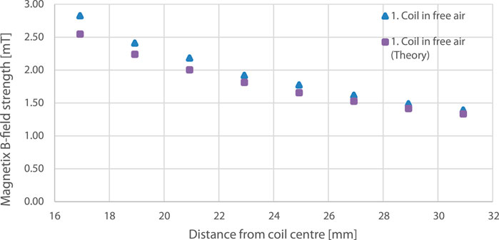
FIGURE 14. Magnetic B-field strength that was measured and the theoretical values computed with Eq. 13.

The results are in good agreement and follow the same trend. A difference of 4%–11% between the theory and the experiment is observed for each measurement. There are several aspects that could be the cause of this difference. Firstly, the theory is based on Direct-Current (DC) while for the experiment Alternating-Current (AC) at a relatively high frequency is used. Secondly, the probe is calibrated in a constant AC magnetic field that differs from the varying magnetic field. Despite theoretically correct averaging of the theoretical data over the inner area of the probe this could differ from reality. Thirdly, a slight position inaccuracy of the probe (e.g., in the order of 0.5 [mm]) will significantly affect the result, especially for the measurements closest to the coil. Because the coil that was used to measure the magnetic field strength has a certain thickness the measurements could not be conducted closer to the coil than 17 [mm].

The results of the magnetic B-field strength measurements and the simulated values via FEA are shown in Figure 15.

FIGURE 15

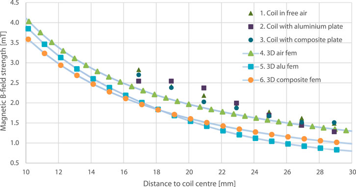
FIGURE 15. Magnetic B-field strength computed at a distance from the coil using a 3 D FEA simulation model that was introduced in Section 2.4 versus the measured values.

The measurements in air and with a composite workpiece are in good agreement. As can be expected the composite plate has a negligible effect on the magnetic field. The measured magnetic B-field strength for the aluminium plate is lower than expected near the coil. The reason has not been determined but may be due to the averaging of B-field strength values of the field probe area that was used to compute the measurement values. Furthermore, as can be seen from the results plotted in Figure 15 the simulated values for the 3D electromagnetic model are close to the values measured near the coil. It is expected that further mesh refinement would improve these results as was shown in previous work with a 2 D model (de Wit, et al., 2022).

4 Experiments to validate the modelling

Inductive heating measurements were carried out to obtain data to compare the numerical simulation model results with measurements on equipment that captures key aspects of our induction welding equipment.

4.1 Experimental setup

The inductive heating measurements were performed on three square plates. The material consisted of Toray TC1320 PEKK AS4D, the ply thickness was approximately 0.138 [mm] and the global dimensions were 400 [mm] x 400 [mm] x 5 [mm]. Three different lay-ups were manufactured, plate A2, a Uni-Directional (UD) [0]₃₆, plate A1, a cross ply [0,90]_9s and plate A3, a cross-ply grouped [0₃,90₃]_3s. The three plates were manufactured via Automatic Fibre Placement (AFP) as three sub packages of 500 [mm] x 500 [mm] UD plates. After AFP these plates were then consolidated inside an autoclave at 8 [bar].

Each plate was placed inside the inductive heating equipment and was supported at the edges by a glass plate. Hence, except for a 30 [mm] support on either side the entire composite plate was hanging freely in the air. The coil was placed at a distance of 14 [mm] above the surface of the plate and was aligned with the center of the plate as shown in Figure 16. The 0° direction was aligned with the length direction of the coil.

FIGURE 16

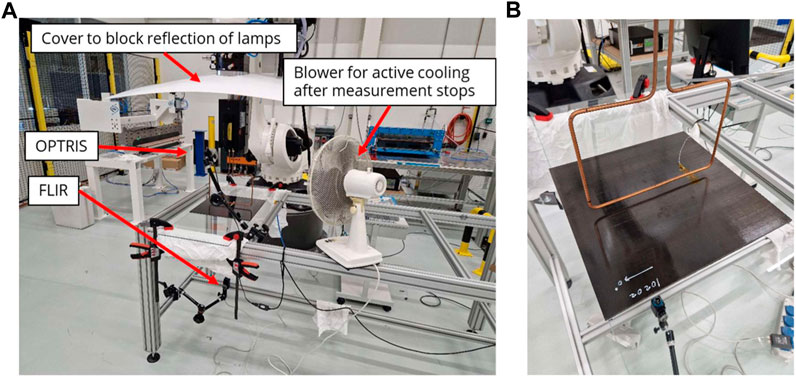
FIGURE 16. Measurement setup for the inductive heating measurements. (A) Key components of the measurement setup. (B) White marking on the laminate corresponds to the 0° ply orientation. Furthermore, the positioning of the thermocouple below the coil can be seen.

The surface temperature of the plate was measured by two infrared (IR) cameras. An Optris PI 640 measured the top of the plate and a FLIR A35 the bottom of the plate. The top camera was positioned at an angle with the plate surface to ensure visibility under the coil, while the bottom camera was positioned perpendicular to the bottom surface. Furthermore, two thermocouples were located at top and bottom at 100 [mm] from the edge of the plate and below the coil (200 [mm] from the other edge). The coil was centred above the plate, 200 [mm] from the far edges and 50 [mm] on either side of the closest edges.

To compare the temperature measurements with the results from the simulation the plate was heated up to a temperature where no melting or other thermal effects that are not part of the modelling were expected. The plate was therefore heated from room temperature (approx. 22 [⁰C]) until 150 [⁰C] and then cooled down to approximately 100 [⁰C]. After reaching 100 [⁰C] the measurement was stopped and a fan was turned on to speed up the cooling process until room temperature. The necessary equipment settings were determined using the [0,90]_9s plate which reached 150 [⁰C] after 37 [s] and then was passively cooled down for another 60 [s] via natural convection. These settings were applied to the other plates as well. A frequency of approximately 194 [kHz] and an Amperage of 199.5 [A] was used for this heating process and was used throughout the other heating experiments as well.

4.2 Measurement and simulation results and discussion

A1 Cross ply [0,90]_9s After some tuning for the top and bottom of each plate a contour plot of the measured temperatures was created and a similar colour spectrum was used for the simulated values. The results are shown in Figure 17.

FIGURE 17

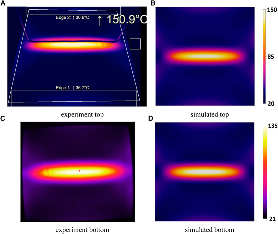
FIGURE 17. Temperature contour plot for the cross ply [0,90]_9s plate (A1). (A–C) correspond to measurements whereas (B–D) correspond to simulated values.

As can be seen from Figure 17 (a) and (c), not only the plate underneath the coil increases in temperature but also the edges of the plate rise in temperature via a pattern that is typical for this plate geometry and coil. Using the FLIR software for the bottom of the plate we did not manage to create more contrast. Still some edge heating can be observed. The contour plots taken from the simulated plate shown in Figure 17 (b) and (d) are in good agreement with the results of the experiments.

From each of the surface measurements the maximum temperatures were taken. In addition, the maximum temperature at the edges further away from the coil were taken and combined in a graph together with the measurements from the thermocouples and the FEM calculated values. The results are shown in Figure 18.

FIGURE 18

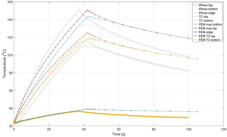
FIGURE 18. Temperature measurements cross-ply [0,90]_9s plate (A1). The surface temperatures were measured via Optris (top surface), FLIR (bottom surface) and two thermocouples placed 100 [mm] from the edge underneath the coil. The FEM values were taken from the simulation model.

The Optris camera recalibrates several times during the measurement and therefore a jump in the recorded temperature is visible. As can be seen from Figure 18 the Optris and FLIR camera measure immediately the turning off of the induction coil whereas the thermocouples require some time to heat up and cool down before measuring a change in temperature. Therefore the peak temperature is a smooth curve on the thermocouple graph rather than the sudden jump that is seen with the IR cameras.

The simulated values are in qualitative agreement with the measured values. The top surface of the plate in the simulation model reached 140 [⁰C] in 37 [s] whereas the measurements showed 151 [⁰C]. Therefore, the simulation of the inductive heating was continued until 42 [s] when the maximum surface temperature was equal to 151 [⁰C]. Furthermore, the difference between top and bottom maximum surface temperature is larger for the experiments (approximately 15 [⁰C]) as compared to the simulated values (approximately 5 [⁰C]). Since conductive thermal properties were taken from literature, rather than measured properties some deviation may be expected there. Finally, as can be seen from the cooling part of the graph, the drop in temperature measured during the experiments is somewhat larger than what was computed. Hence, the film coefficients applied to the model to represent the convective cooling should be a bit higher than those that were computed.

A2, Uni-Directional (UD) [0]₃₆ The UD plate is expected not to heat up at all. Since all plies are running parallel to the coil there is no current return path via cross-ply interfaces. However, some plies might be in contact in longitudinal direction. Simulations of this type of plate suggest heating due to small eddy currents that are generated in the laminate supposedly due to a non-zero electric conductivity in the longitudinal fiber direction. Hence, plate A2 was used to prove that this phenomenon occurs in practice. As can be seen from the thermal images in Figure 19 there is a slight increase in temperature at the edges of the plate

FIGURE 19

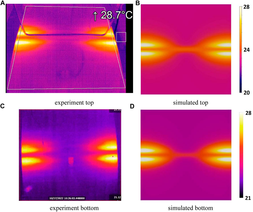
FIGURE 19. Temperature contour plot for the UD [0]₃₆ plate (A2). (A–C) Some increment in temperature is observed near the edges of the plate. (B–D) Temperature contour plot from the simulations.

The edges of the plate contribute to generation of a current return path and corresponding joule heating. The simulation model shows a similar heating pattern. For completeness, the measured and calculated temperatures as recorded for the A2 plate are shown in Figure 20.

FIGURE 20

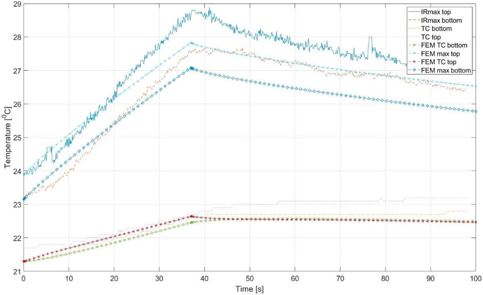
FIGURE 20. Recorded and computed temperatures for the UD [0]₃₆ plate (A2).

Note that the maximum temperatures are located near the edges of the plate instead of underneath the coil. Furthermore, the thermocouples that are placed 100 [mm] away from the edge underneath the coil record only a minor increase in temperature, approximately 1.5 [⁰C] whereas the maximum temperature at the top increases to almost 29 [⁰C] from room temperature (23 [⁰C]). Furthermore, as we can see from the temperature graph the top and bottom maximum recorded values differ slightly as well as the thermocouple values. This is partly due to the fact that the Optis and FLIR camera did not register the same room temperature and always showed a difference of approximately 1 [⁰C]. We did not locate any other heat sources that would cause the top of the plate to be warmer than the bottom. During the heating of the other two plates A1 and A3 this temperature difference was not an issue but for this case the difference is visible in the graph.

Comparing the simulated values with those recorded during the measurements the values are in good agreement. In both the experiment and the simulation the heating was 37 [s] and the difference in maximum temperature is only 1.5 [⁰C]. The results for the thermocouples are in good agreement although the temperature increment is very little.

A3, a grouped cross-ply [0₃,90₃]_3s The third plate consisted of less cross-ply interfaces and initially we expected via coarse mesh FE analysis that this plate would heat up less than the cross-ply plate A1. The A1 plate has 34 cross-ply interfaces, whereas the A3 plate has only 10 cross-ply interfaces. However, the temperature plot in Figure 21 shows that after 37 [s] of inductive heating the plate reached a temperature of approximately 155 [⁰C] which is roughly the same temperature as the A1 plate (recall Figure 17) that reached 151 [⁰C].

FIGURE 21

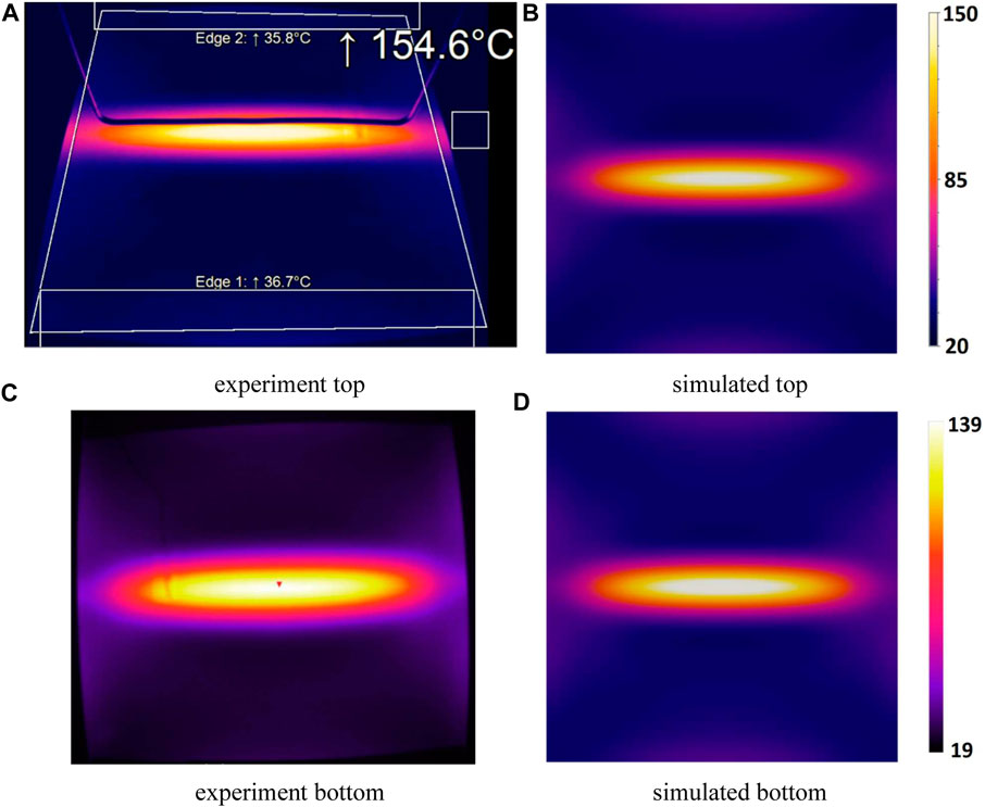
FIGURE 21. Temperature plot of top and bottom temperatures of the grouped cross-ply [0₃,90₃]_3s plate (A3). (A) and (C) correspond to measurements whereas (B) and (D) correspond to simulated values.

One possibility is that in addition to the cross-ply interfaces having an effect on the surface temperature also the current penetration depth (Christopoulos, 1990) is of influence. The higher the electric conductivity of the workpiece the less deep the eddy currents penetrate and instead form at the surface of the workpiece. This would lead to higher top surface temperatures. Through conduction effects within the laminate the bottom surface temperature could then also increase. For the A3 plate the bottom surface temperature is slightly higher than that of the A1 plate as can be seen in Figure 22 that shows a recording of the maximum IR measurements and the thermocouple measurements for the A3 plate.

FIGURE 22

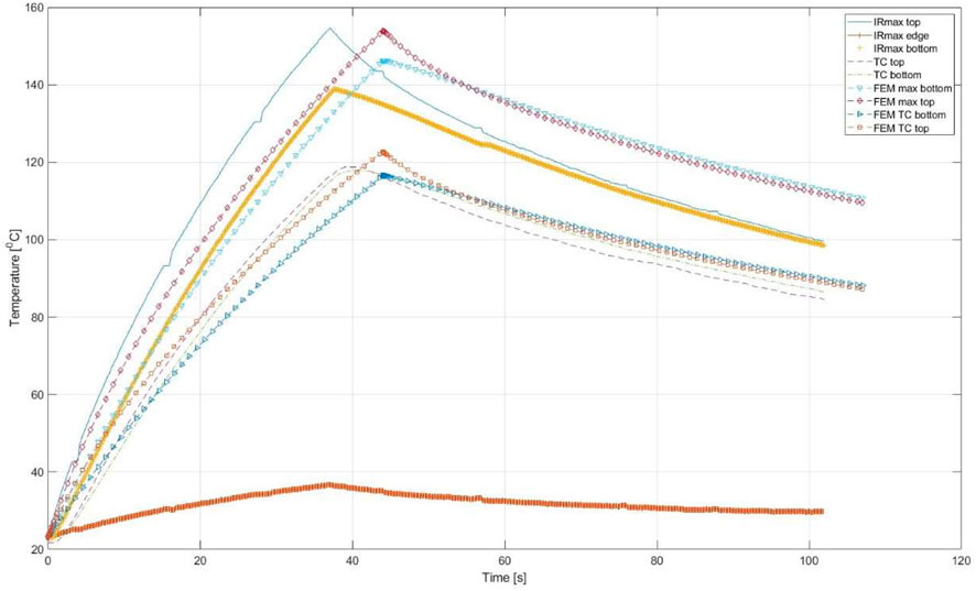
FIGURE 22. Temperature measurements of the grouped cross-ply [0₃,90₃]_3s plate (A3).

The top of the plate reaches a maximum temperature of approximately 155 [⁰C] and the bottom a temperature of approximately 139 [⁰C]. For the A1 plate the top reached 151 [⁰C] and the bottom 136 [⁰C]. Hence, the difference between the two measurements is small and therefore both plates are considered to heat up similarly. A probable cause could be that the number of cross-ply interfaces does not have to be significant in order for a relatively thick laminate to heat up.

For the simulated A3 plate the maximum temperature reaches 151 [⁰C] after 44.6 [s] whereas the A1 plate reached 151 [⁰C] after 44 [s]. Furthermore, in the simulation for plate A3 after 37 [s] the temperature is 138 [⁰C]. For plate A1 in the simulation for the plate A1 after 37 [s] the temperature is 140 [⁰C]. Hence, in the simulations the A1 plate heats up slightly faster than the A3 plate. However, this difference is considered small and may be also due to the mesh not capturing every effect as we could not further refine the mesh for such a thick plate.

5 Conclusions and further work

Several experimental tests were developed to obtain material properties and verify the electromagnetic simulation approach. The measured material properties were compared with data found in literature and showed good agreement. The results of the magnetic field measurements and applied load on the coil supported the modelling steps for building the electromagnetic FE model. The thermal experiments showed that increasing the number of cross-ply interfaces may not always lead to higher temperature at the laminate upper and lower surfaces. Finally, the results from the simulations were in good agreement with the data recorded for the thermal experiments. Some further improvements in the modelling require the measuring of each relevant material property of the material over the relevant temperature range. The authors intend to further improve on the developed measurement techniques to include through the thickness measurements of the electrical conductance and to develop a simplified 3D FE model that is less computationally demanding than the current 3D approach. The results of the present work will be used for further investigation of inductive welding of long and slender joins.

Data availability statement

The raw data supporting the conclusion of this article will be made available by the authors, without undue reservation.

Author contributions

AdW and WV contributed to conception and design of the study. NvH and LS setup the experiments and recorded the data. AdW wrote the first draft of the manuscript. NvH and WV wrote sections of the manuscript. All auteurs contributed to manuscript revision.

Funding

This project has received funding from the Clean Sky 2 Joint Undertaking (JU) under grant agreement No 945583. The JU receives support from the European Union’s Horizon 2020 research and innovation programme and the Clean Sky 2 JU members other than the Union.

Conflict of interest

The authors declare that the research was conducted in the absence of any commercial or financial relationships that could be construed as a potential conflict of interest.

Publisher’s note

All claims expressed in this article are solely those of the authors and do not necessarily represent those of their affiliated organizations, or those of the publisher, the editors and the reviewers. Any product that may be evaluated in this article, or claim that may be made by its manufacturer, is not guaranteed or endorsed by the publisher.

References

Ahmed, T., Stavrov, D., Bersee, H., and Beukers, A. (2006). Induction welding of thermoplastic composites - an overview. Compos. Part A Appl. Sci. Manuf. 37, 1638–1651. doi:10.1016/j.compositesa.2005.10.009

CrossRef Full Text | Google Scholar

Buser, Y., Bieleman, G., Wijskamp, S., and Akkerman, R. (2022). “Characterisation of orthotropic electrical conductivity of unidirectional c/paek thermoplastic composites,” in Proceedings of the 20th European Conference on Composite Materials - Composites Meet Sustainability, Lausanne, Switzerland, June 2022.

Google Scholar

Chen, L. (2016). Finite element methods for Maxwell equations. Oakland, CA, USA: University of California.

Google Scholar

Cheng, J., Wang, B., Xu, D., Qiu, J., and Takagi, T. (2021). Resistive loss considerations in the finite element analysis of eddy current attenuation in anisotropic conductive composites. NDT E Int. 119–102403. doi:10.1016/j.ndteint.2021.102403

CrossRef Full Text | Google Scholar

Christopoulos, C. (1990). An introduction to applied electromagnetism. Toronto, OA, Canada: Wiley.

Google Scholar

de Wit, A. J., van Hoorn, N., Nahuis, B. R., and Vankan, W. J. (2022a). “Numerical simulation of eddy current generation in uni-directional thermoplastic composites,” in Proceedings of the 20th European Conference on Composite Materials - Composites Meet Sustainability, Lausanne, Switzerland, June 2022.

Google Scholar

de Wit, A. J., van Hoorn, N., Nahuis, B. R., and Vankan, W. J. (2021). Prediction of thermo-mechanic effects through numerical simulation of induction heating of thermoplastic composites. Amsterdam, Netherlands: Royal Netherlands Aerospace Centre - NLR.

Google Scholar

de Wit, A. J., van Hoorn, N., Straathof, L. S., and Vankan, W. J., 2022b. Eddy current simulation and experiments for assessments of inductive heating in uni-directional thermoplastic composites. International Congress on Welding Additive Manufacturing and associated Non Destructive Testing, June 2022, Paris, France, .

Google Scholar

Grouve, W., Vruggink, E., Sacchetti, F., and Akkerman, R. (2020). Induction heating of UD C/PEKK cross-ply laminates. Procedia Manuf. 47, 29–35. doi:10.1016/j.promfg.2020.04.112

CrossRef Full Text | Google Scholar

Kim, H. J., Yarlagadda, S., Shevchenko, N. B., Fink, B. K., and Gillespie, J. W. (2000). Development of a numerical model to predict in-plane heat generation patterns during induction processing of carbon fiber-reinforced prepreg stacks. Jounral Compos. Mater. 37 (16), 1461–1483. doi:10.1177/0021998303034460

CrossRef Full Text | Google Scholar

Moser, L. (2012). Experimental analysis and modeling of susceptorless induction welding of high performance thermoplastic polymer composites. Kaiserslautern, Germany: Kaiserslautern: Institute für Verbundwerkstoffe GmbH. PhD thesis.

O'Shaughnessey, P. G., Dubé, M., and Villegas, I. F. (2016). Modeling and experimental investigation of induction welding of thermoplastic composites and comparison with other welding processes. J. Compos. Mater. 50 (21), 2895–2910. doi:10.1177/0021998315614991

CrossRef Full Text | Google Scholar

Simulia, (2023). Abaqus 2023 theory manual. Rhode Island: Dassault Systèmes Simulia Corp.

Google Scholar

Xu, X., Ji, H., Qui, J., Cheng, J., Wu, Y., and Takagi, T. (2018). Interlaminar contact resistivity and its influence on eddy currents in carbon fiber reinforced polymer laminates. NDT E Int. 94, 79–91. doi:10.1016/j.ndteint.2017.12.003

CrossRef Full Text | Google Scholar

Yousefpour, A., Hojjati, M., and Immarigeon, J.-P. (2004). Fusion bonding/welding of thermoplastic composites. J. Thermoplast. Compos. Mater. 17, 303–341. doi:10.1177/0892705704045187

CrossRef Full Text | Google Scholar

Yousefpour, A., and Hojjati, M. (2011). Welding thermoplastics and thermoplastic composite materials. Hoboken, NJ, US: John Wiley& Sons.

Google Scholar