Physics-based manifold learning in scaffolds for tissue engineering: Application to inverse problems

In the field of bone regeneration, insertion of scaffolds favours bone formation by triggering the differentiation of mesenchymal cells into osteoblasts. The presence of Calcium ions (Ca²⁺) in the interstitial fluid across scaffolds is thought to play a relevant role in the process. In particular, the Ca²⁺ patterns can be used as an indicator of where to expect bone formation. In this work, we analyse the inverse problem for these distribution patterns, using an advection-diffusion nonlinear model for the concentration of Ca²⁺. That is, given a set of observables which are related to the amount of expected bone formation, we aim at determining the values of the parameters that best fit the data. The problem is solved in a realistic 3D-printed structured scaffold for two uncertain parameters: the amplitude of the velocity of the interstitial fluid and the ionic release rate from the scaffold. The minimization in the inverse problem requires multiple evaluations of the nonlinear model. The computational cost is alleviated by the combination of standard Proper Orthogonal Decomposition (POD), to reduce the number of degrees of freedom, with an adhoc hyper-reduction strategy, which avoids the assembly of a full-order system at every iteration of the Newton’s method. The proposed hyper-reduction method is formulated using the Principal Component Analysis (PCA) decomposition of suitable training sets, devised from the weak form of the problem. In the numerical tests, the hyper-reduced formulation leads to accurate results with a significant reduction of the computational demands with respect to standard POD.

1 Introduction

Material-associated osteoinduction is the process by which steam cells differentiate into osteoblasts due to their interaction with the material conforming bone graft substitutes or scaffolds. Scaffolds are biocompatible structures that support bone formation when inserted into a proper physiological environment. The causes behind osteoinduction are not completely understood, and identifying the material properties that stimulate cell differentiation and favour bone regeneration is of major interest in tissue engineering. Some of the factors behind osteoinduction have been related to the architecture or morphology of the material (that is, its microstructure and porosity), its chemical composition, and the presence of calcium (Ca²⁺) and phosphate ions in the interstitial fluid (Ripamonti et al., 2007; Danoux et al., 2015; Habraken et al., 2016; Bohner et al., 2022). Also, Ca²⁺ gradients are related to cell migration and osteoinductive differentiation (Tang et al., 2018). Analysing the distribution of ions through scaffolds is therefore crucial to determine the effect that different physical and geometrical parameters can have on osteoinduction.

Numerical simulation enables to test different designs and compositions while reducing experimental costs, with the final objective of reducing in vivo and in vitro experimentation to a minimum (Santamaría et al., 2013; Guyot et al., 2014; Van hede et al., 2021). In this framework, a multiparametric advection-diffusion nonlinear model for the concentration of Ca²⁺ ions across calcium phosphate scaffolds is proposed in Muixí et al. (2022). The Ca²⁺ steady-state distribution is there viewed as an indicator of where to expect bone formation for different material configurations. Actually, the highly-crowded regions in the numerical simulations qualitatively agree with the patterns of bone growth in experimental observations by Barba et al. (2017). The model in Muixí et al. (2022) accounts for six physical parameters which are difficult to estimate, related to the diffusivity of the ions, the velocity and the viscosity of the interstitial fluid and the release rate of ions from the scaffold. The value of each parameter ranges in a large interval accounting for uncertainty in the input data.

The goal of this work is to study the associated inverse problem: given a set of observables or observational data for a final Ca²⁺ distribution, we aim to identify the value of the parameters in the model that best fit the observations. With this, we would be able to estimate the value of uncertain parameters given the experimental outcome for some configuration. This is done through the definition of a cost functional that quantifies the misfit between the outcome of the simulation and the observables. The minimization of this functional requires multiple evaluation of the parametric model, which leads to a high computational cost. For illustrative purposes, we restrict ourselves to the identification of two parameters: the velocity amplitude of the interstitial fluid and the release rate of Ca²⁺ from the scaffold, which are the parameters leading to more differentiated patterns.

The numerical efforts in the minimization can be reduced with a Reduced Order Modelling (ROM) formulation of the problem. Here, we apply the widely used Proper Orthogonal Decomposition (POD) (Berkooz et al., 1993; Patera and Rozza, 2007; Quarteroni and Rozza, 2014; Díez et al., 2021). POD discovers a linear space of low dimension embedding the manifold of parametric solutions by doing a Principal Component Analysis (PCA) of a precomputed family of solutions (the training set). Afterwards, the PCA low-order basis is used to approximate the solution in subsequent evaluations of the model, significantly reducing the number of degrees of freedom.

Nevertheless, in the case of nonlinear models, POD fails to drastically reduce the computational cost. In a standard POD formulation, we first build the full-order system of equations and then project it into the PCA reduced space. For nonlinear systems, this means assembling a full-order system at every iteration of, for instance, the Newton’s method scheme. To remedy this issue, several hyper-reduction methods have been proposed, including the Discrete Empirical Interpolation Method (DEIM) (Chaturantabut and Sorensen, 2010; Negri et al., 2015), the Best Points Interpolation Method (BPIM) (Nguyen and Peraire, 2008), among others. Here, the POD is combined with an adhoc hyper-reduction technique to estimate the nonlinear contributions, which is also based in the PCA of suitable training sets and offers an easy-to-implement strategy to build the reduced systems in the Newton’s formulation of the problem.

This paper is structured as follows. In Section 2, the forward and the inverse problems are presented, as well as the employed reduced-order methodology. The POD formulation is summarized in Section 2.2.1 and the adhoc hyper-reduction technique is described in 2.2.2. In Section 3, numerical results for the inverse problem are shown in a realistic domain, based on a 3D-printed calcium phosphate structured scaffold. Finally, the main results and the limitations of the strategy are discussed in Section 4.

2 Materials and methods

2.1 Problem statement

We consider the multiparametric advection-diffusion nonlinear model proposed in Muixí et al. (2022) for the concentration of Ca²⁺ in the interstitial fluid that passes through a scaffold. The model accounts for the scaffold releasing ions in the interstitial fluid and the fluid dragging them, changing the concentration distribution. Bone formation is expected in regions with a high concentration of Ca²⁺. Here, the parametrisation is given by the velocity amplitude of the fluid, υ, and the Ca²⁺ release rate from the scaffold into the surrounding fluid, r, which are parameters with a significant effect on the amount of expected bone formation.

We aim to infer the value of the parameters, υ and r, given a set of observables (or outcomes) associated to the concentration of Ca²⁺, by solving the corresponding inverse problem. The multiple model evaluation needed to solve the inverse problem motivates the use of a ROM technique to accelerate the computation. Due to the nonlinear character of the model, we combine the Proper Orthogonal Decomposition (POD) to reduce the dimension of the systems, with an adhoc hyper-reduction strategy to make the assembly process more efficient.

The problem is solved in a realistic domain based on a 3D-printed structured calcium phosphate scaffold, see Figure 1. This geometry was first developed and experimentally tested for osteoinduction in intramuscular implantation by Barba et al. (2017). The scaffold has a geometrically structured distribution, with regular pores with an average size of 289 μm and a porosity of 54.1%. We consider a representative volume of dimensions 1930 × 2040 × 1960μm³.

FIGURE 1

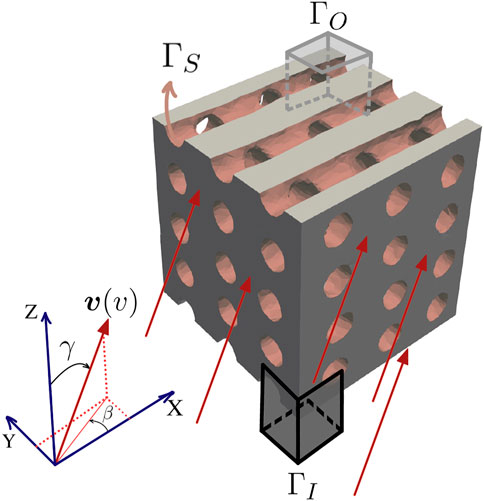
FIGURE 1. Domain for the interstitial fluid across a representative volume of the 3D-printed structured scaffold. The three dark grey faces (through the origin) mark the inlet faces, Γ_I, where Dirichlet conditions are set to 0. The opposite light grey faces correspond to the outlet, Γ_O. Light red surfaces indicate the scaffold-fluid interface, Γ_S, where the release Robin conditions are imposed.

2.1.1 Forward problem and parametrization

The steady nonlinear advection-diffusion problem reads

$\left\{\begin{array}{cccccc}\hfill & -\mathbf{\nabla }\cdot \left(\nu \left(c\right)\mathbf{\nabla }c\right)+\mathit{\upsilon }\cdot \mathbf{\nabla }c=0\hfill & \hfill & \text{in}\hfill & \hfill & \mathrm{\Omega },\hfill \\ \hfill & c=0\hfill & \hfill & \text{on}\hfill & \hfill & {\mathrm{\Gamma }}_I,\hfill \\ \hfill & \mathbf{\nabla }c\cdot \mathit{n}=0\hfill & \hfill & \text{on}\hfill & \hfill & {\mathrm{\Gamma }}_O,\hfill \\ \hfill & -\nu \left(c\right)\mathbf{\nabla }c\cdot \mathit{n}=r\left(c-1\right)\hfill & \hfill & \text{on}\hfill & \hfill & {\mathrm{\Gamma }}_S,\hfill \end{array}\right.(1)$

where c is the adimensional concentration of Ca²⁺ (normalized to the maximum value of 1), and Ω ⊂ IR³ is the domain through the scaffold occupied by the intersitital fluid. The boundary ∂Ω is partitioned into $\partial \mathrm{\Omega }=\overline{{\mathrm{\Gamma }}_I}\cup \overline{{\mathrm{\Gamma }}_O}\cup \overline{{\mathrm{\Gamma }}_S}$, being Γ_I the inlet of the fluid, Γ_O the outlet and Γ_S the part of the boundary in contact with the scaffold, as shown in Figure 1. In the equations, ν(c) is the diffusivity, υ≔υ(x; υ) is the advection velocity and υ denotes its amplitude (see Eq. 4), r is the Ca²⁺ release rate from the scaffold, and n stands for the outward unit normal vector. We account for the uncertainty and variability of two parameters: υ and r.

On the inlet Γ_I, Dirichlet boundary conditions are set to zero to simulate the entry of clean interstitial fluid in the domain and to avoid upstream diffusion against the flow direction. On the outlet Γ_O, homogeneous Neumann boundary conditions are imposed. On Γ_S, which is the solid-fluid interface, we impose Robin boundary conditions with ionic release rate r. A higher (positive) value of r implies a faster relase of ions from the scaffold into the fluid. Note that the Robin condition sets a saturation concentration of c = 1. For this analysis, r is parametrised in the range I_r = [5, 20]μm/s.

The expression for the concentration-dependent diffusivity ν(c) is

$\nu \left(c\right)=D_{\mathrm{SE}}10^{-c},(2)$

where D_SE is the constant Stokes-Einstein diffusion coefficient for Ca²⁺, obtained as

$D_{\mathrm{SE}}=\frac{k_{B}T}{6\pi \eta \rho },(3)$

with k_B = 1.38 ⋅ 10^–23 JK⁻¹ the Boltzmann constant, T = 37°C the temperature, ρ = 114 pm the ionic radius of Ca²⁺ (Manhas et al., 2017) and η = 1.2 ⋅ 10^–3 Pa⋅s the viscosity of the fluid, which is taken in the range of blood plasma’s viscosity (Késmárky et al., 2008). With the diffusivity law in (Eq. 2), an increase in the concentration c implies a decrease in the diffusivity. Actually, diffusivity is reduced by one order of magnitude in fully crowded regions (where c = 1), when compared to regions without Ca²⁺ (where c = 0).

The advection velocity υ is an input for the problem. It is expressed as a combination of normalized velocity fields υ_x, υ_y and υ_z, coming from potential flows in X, Y and Z directions, respectively, that is

$\mathit{\upsilon }\left(\mathit{x};\upsilon \right)=\upsilon \left(\sin \gamma \cos \beta {\mathit{\upsilon }}_x\left(\mathit{x}\right)+\sin \gamma \sin \beta {\mathit{\upsilon }}_y\left(\mathit{x}\right)+\cos \gamma {\mathit{\upsilon }}_z\left(\mathit{x}\right)\right),(4)$

with υ the velocity amplitude and combination angles $\gamma =\beta =\frac{\pi }{4}$. The amplitude v varies in the interval I_υ = [1, 60]μm/s.

The intervals for the two parameters, namely I_r and I_υ, are chosen in Muixí et al. (2022) by numerical experimentation, covering cases in which the final distribution presents highly differentiated patterns.

2.1.2 Newton’s method formulation

The nonlinear Boundary Value Problem (BVP) (Eq. 1) is solved using Newton’s method. Given an initial guess to the solution, c⁰, we seek a succession of approximations c^k+1 = c^k + δc for k = 0, 1, … until convergence. For parameters υ and r, the weak form of the kth Newton iteration reads: given an approximation c^k ∈ V, with $V=\{w\in H^1(\mathrm{\Omega }):w{|}_{{\mathrm{\Gamma }}_I}=0\}$, find δc ∈ V such that

$\begin{array}{cc}\hfill a_1\left(\delta c,c^k,w\right)+a_2\left(\delta c,c^k,w\right)& +a_3\left(\delta c,w;\upsilon \right)+a_4\left(\delta c,w;r\right)\hfill \\ \hfill & =-\left(a_1\left(c^k,c^k,w\right)+a_3\left(c^k,w;\upsilon \right)\right.\hfill \\ \hfill & \left.+a_4\left(c^k,w;r\right)-a_4\left(1,w;r\right)\right)\hfill \\ \hfill & \forall w\in V,\hfill \end{array}(5)$

with

$\begin{array}{cc}\hfill & a_1\left(\delta c,c^k,w\right)={\int }_{\mathrm{\Omega }}\nu \left(c^k\right)\mathbf{\nabla }\delta c\cdot \mathbf{\nabla }w\mathrm{d}\mathrm{\Omega },\hfill \\ \hfill & a_2\left(\delta c,c^k,w\right)={\int }_{\mathrm{\Omega }}{\nu }^{\prime }\left(c^k\right)\delta c\mathbf{\nabla }{c}^k\cdot \mathbf{\nabla }w\mathrm{d}\mathrm{\Omega },\hfill \\ \hfill & a_3\left(\delta c,w;\upsilon \right)={\int }_{\mathrm{\Omega }}\mathit{\upsilon }\cdot \mathbf{\nabla }\delta cw\mathrm{d}\mathrm{\Omega },\hfill \\ \hfill & a_4\left(\delta c,w;r\right)={\int }_{{\mathrm{\Gamma }}_S}r\delta cw\mathrm{d}\mathrm{\Gamma },\hfill \end{array}(6)$

and then set c^k+1 = c^k + δc. We use the notation ${\nu }^{\prime }(c)=\frac{\mathrm{d}\nu }{\mathrm{d}c}(c)$. The initial guess c⁰ is taken as the solution for the linear case with constant diffusivity ν = D_SE.

The discretization of (Eq. 5) leads to a system of the form

$\mathit{K}\left({\mathit{c}}^k;\mathit{\mu }\right)\mathit{\delta }\mathit{c}=\mathit{f}\left({\mathit{c}}^k;\mathit{\mu }\right),(7)$

with c^k and δc the vectors of nodal values for c^k and δc, respectively, and μ = (υ, r) the parameters in the model. Convergence is reached when both the relative values of the Euclidean norm of δc and of the residual f(c^k; μ) are below some tolerance, here set to 10^–6. Due to the nonlinear dependence on c of the weak form of the problem (Eq. 6), the system has to be assembled at every iteration k. In order to effectively reduce the cost, we reduce the number of unknowns in (Eq. 7) using POD. In a nonlinear context, POD reduction is not sufficient and in order to properly approximate the nonlinear contributions in K(c^k; μ) and f(c^k; μ), an adhoc hyper-reduction technique is devised in Section 2.2.

2.1.3 Observables

Regions with high concentrations of Ca²⁺ are the regions where we expect bone formation. Actually, in Muixí et al. (2022), highly-concentrated regions present qualitatively similar patterns to those of bone growth in the experiments by Barba et al. (2017). Thus, we assume that the amount of formed bone for a parametric setting is characterized through the volumes of regions with a minimum Ca²⁺ concentration and the total concentration in the domain.

We define four observables, or quantities of interest, for a given concentration field c. Three observables account for the relative volumes occupied with minimum concentration thresholds β = 0.1, 0.5 and 0.9, namely

$V_{\beta }\left(c\right)=\left|{\mathrm{\Omega }}_{\beta }\right|/\left|\mathrm{\Omega }\right|,(8)$

where $\left|\mathrm{\Omega }\right|$ stands for the volume of the domain Ω and

${\mathrm{\Omega }}_{\beta }=\left\{\mathit{x}\in \mathrm{\Omega }:c\left(\mathit{x}\right)>\beta \right\}.(9)$

The normalized total concentration of Ca²⁺ in the domain is computed as

$V_{\mathrm{T}}\left(c\right)=\frac{1}{|\mathrm{\Omega }|}{\int }_{\mathrm{\Omega }}c\mathrm{d}\mathrm{\Omega },(10)$

where the normalization accounts for the maximum value of concentration, c = 1, as stated by the Robin boundary condition on Γ_S in the system of Eq. 1.

The vector containing the observables for a given concentration field c(υ, r) is denoted by

$\mathit{V}\left(\upsilon ,r\right)=\left(V_{0.1}\left(c\right),V_{0.5}\left(c\right),V_{0.9}\left(c\right),V_{\mathrm{T}}\left(c\right)\right).(11)$

Note that these four observables are adimensional and take values between 0 and 1.

2.1.4 Inverse problem

The inverse problem consists in identifying the parameters υ and r that minimize the discrepancy between some given observables V^∗ and the outcome of the parametric model V(υ, r). This discrepancy is quantified through the functional $\mathcal{J}(\upsilon ,r)$, defined as

$\mathcal{J}\left(\upsilon ,r\right)=\Vert {\mathit{V}}^{\ast }-\mathit{V}\left(\upsilon ,r\right)\Vert ,(12)$

where ‖⋅‖ stands for the Euclidean norm. Thus, the inverse problem over the parametric space reads: given V^∗, find υ^∗ ∈ I_υ and r^∗ ∈ I_r such that

$\left({\upsilon }^{\ast },r^{\ast }\right)=\underset{\upsilon \in I_{\upsilon },r\in I_r}{\mathrm{argmin}}\mathcal{J}\left(\upsilon ,r\right).(13)$

The minimization requires multiple evaluations of the forward problem (Eq. 1), corresponding to different values of the parameters. The numerical methodology described in Section 2.2 aims at making this computation efficient.

2.2 Numerical methodology

The multiple evaluations required in solving the inverse problem (Eq. 13) call for the use of a reduced-order strategy to reduce the computational cost. For any given parameters μ = (υ, r), the solution is computed with the Newton’s method, iteratively solving the linear system of Eq. 7 until convergence. In order to make each evaluation more efficient, we propose:

• using the Proper Orthogonal Decomposition (POD) to reduce the number of unknowns in Eq. 7, and

• approximating the nonlinear contributions in K(c^k; μ) and f(c^k; μ) with an adhoc hyper-reduction technique, thus avoiding the assembly of the full-order system at every iteration.

2.2.1 Proper orthogonal decomposition

Solutions of a parametric problem with n_p parameters lie in a manifold of low dimension, equal to the number of independent parameters, which is embedded in the larger space ${\mathrm{I}\mathrm{R}}^{n_d}$, with n_d the number of degrees of freedom in the discretization. POD discovers a linear space of dimension n_k, with n_p ≤ n_k ≪ n_d, including the manifold of parametric solutions, by performing a Principal Component Analysis (PCA) of a precomputed family of solutions or snapshots (the training set). Then, for subsequent evaluations of the model, the solution of the system is approximated in the PCA linear subspace of dimension n_k, readily reducing the number of unknowns from n_d to n_k by following a Reduced Basis approach.

The training set is defined as the solutions of the nonlinear full-order problem (Eq. 1) corresponding to a representative sampling of the parametric space, given by μⁱ for i = 1, …, n_S, with n_S < n_d. These solutions or snapshots are denoted by xⁱ = c(μⁱ). Snapshots are centered as

${\widehat{\mathit{x}}}^i={\mathit{x}}^i-\bar{\mathit{x}},(14)$

for i = 1, …, n_S, where $\bar{\mathit{x}}$ stands for the mean of the snapshots defined as

$\bar{\mathit{x}}=\frac{1}{n_S}\sum _{i=1}^{n_S}{\mathit{x}}^i.(15)$

Centered snapshots are then collected in a matrix $\mathit{X}\in {\mathrm{I}\mathrm{R}}^{n_d\times n_S}$, this is,

$\mathit{X}=\left[{\widehat{\mathit{x}}}^1{\widehat{\mathit{x}}}^2\dots {\widehat{\mathit{x}}}^{n_S}\right].(16)$

Centering the snapshots is recommended to improve the numerical properties of PCA.

The PCA, which is based on the Singular Value Decomposition (SVD), is used to eliminate redundancies in X. The SVD of X reads

$\mathit{X}=\mathit{U}\mathbf{\Sigma }{\mathit{V}}^{\mathsf{\text{T}}},(17)$

with $\mathit{U}\in {\mathrm{I}\mathrm{R}}^{n_d\times n_d}$ and $\mathit{V}\in {\mathrm{I}\mathrm{R}}^{n_S\times n_S}$ two unitary matrices, and $\mathbf{\Sigma }\in {\mathrm{I}\mathrm{R}}^{n_d\times n_S}$ a diagonal matrix containing the singular values of X in descendent order, ${\sigma }_1\ge {\sigma }_2\ge \cdots \ge {\sigma }_{n_S}\ge 0$. The first n_S columns of U define an orthonormal basis for the linear subspace generated by the snapshots. In order to keep only the relevant information, we choose n_k such that

$\sum _{i=1}^{n_k}{\sigma }_i\ge \left(1-\epsilon \right)\sum _{i=1}^{n_S}{\sigma }_i,(18)$

for some tolerance ɛ. The linear space spanned from the n_k first columns of U, assembled in a matrix ${\mathit{U}}^{\star }\in {\mathrm{I}\mathrm{R}}^{n_d\times n_k}$, approximates the linear space that contains the manifold of snapshots, up to tolerance ɛ.

For a new parametric point μ which is not in the training set, the solution c is approximated by

$\mathit{c}\simeq \bar{\mathit{x}}+{\mathit{U}}^{\star }\mathit{z}=\bar{\mathit{x}}+\sum _{i=1}^{n_k}{\mathit{u}}^i{z}^i,(19)$

for some coefficients $\mathit{z}\in {\mathrm{I}\mathrm{R}}^{n_k}$. In the same way, we approximate

$\mathit{\delta }\mathit{c}\simeq {\mathit{U}}^{\star }\mathit{\delta }\mathit{z}=\sum _{i=1}^{n_k}{\mathit{u}}^i\delta z^i,(20)$

in the n_d × n_d system of Eq. 7, with z the new vector of unknowns. The POD reduced system becomes

$\begin{array}{cc}\hfill & \left[{\mathit{U}}^{\star \mathsf{\text{T}}}\mathit{K}\left({\mathit{c}}^k;\mathit{\mu }\right){\mathit{U}}^{\star }\right]\mathit{\delta }\mathit{z}={\mathit{U}}^{\star \mathsf{\text{T}}}\mathit{f}\left({\mathit{c}}^k;\mathit{\mu }\right),\hfill \\ \hfill & {\mathit{c}}^{k+1}={\mathit{c}}^k+{\mathit{U}}^{\star }\mathit{\delta }\mathit{z},\hfill \\ \hfill & {\mathit{z}}^{k+1}={\mathit{z}}^k+\mathit{\delta }\mathit{z},\hfill \end{array}(21)$

which is a system with n_k equations and n_k unknowns.

2.2.2 Adhoc hyper-reduction strategy based on PCA

The n_k × n_k POD reduced system (21) depends on the solution c^k from the previous iteration in the Newton scheme, as well as on the parameters of the model μ = (υ, r). Using standard POD, we need to assemble the full-order K (c^k; μ) and f(c^k; μ) at every iteration of the Newton scheme, as the approximation of the solution c^k is updated, and then reduce them by multiplying by ${\mathit{U}}^{\star \mathsf{\text{T}}}$.

In order to circumvent the computational expense from assembling the full-order system at every iteration, we propose an adhoc hyper-reduction strategy to approximate the nonlinear contributions in K(c^k; μ) and f(c^k; μ). Following the same philosophy as in POD, we aim to approximate the nonlinear contributions as a linear combination of reduced precomputed matrices and vectors, of dimension n_k × n_k and n_k × 1, respectively. These matrices and vectors are assembled from the PCA reduced bases of suitable training sets, which are defined next based on the expressions of the bilinear forms in the Newton weak formulation (Eq. 5).

All terms in formulation (Eq. 5) are linear with respect to c^k, ν(c^k) or ν(c^k)$\mathbf{\nabla }$c^k. In particular, note that from the diffusivity law in (Eq. 2) we have

${\nu }^{\prime }\left(c\right)=-\ln \left(10\right)\nu \left(c\right).(22)$

To simplify the notation, we define

$y\left(c\right)≔\nu \left(c\right),(23)$

and

$\mathit{g}\left(c\right)≔\nu \left(c\right)\mathbf{\nabla }c.(24)$

The nodal evaluation of these expressions leads to vectors $\mathit{y}(\mathit{c})\in {\mathrm{I}\mathrm{R}}^{n_d}$ and $\mathit{g}(\mathit{c})\in {\mathrm{I}\mathrm{R}}^{3n_d}$, accounting for the three components of g(c) at every node of the finite-element mesh. We compute the gradient on the nodes by means of an L² projection.

In the Newton’s algorithm, matrices and vectors that are linear with respect to c^k are approximated using the POD approximation of c^k in (Eq. 19), which is obtained from the snapshots xⁱ, with i = 1, …, n_S, through the PCA decomposition of the training set matrix $\mathit{X}\in {\mathrm{I}\mathrm{R}}^{n_d\times n_S}$ (Eq. 16). Analogously, to approximate the terms which are linear with respect to y(c^k) or g(c^k), we define two additional training sets, Y and G.

First, we consider yⁱ = y(xⁱ), for i = 1, …, n_S, computed by the nodal evaluation of the diffusivity law (Eq. 2). Following the same notation as in Section 2.2.1, these vectors are centered with mean $\bar{\mathit{y}}$, and they are then collected in matrix $\mathit{Y}\in {\mathrm{I}\mathrm{R}}^{n_d\times n_S}$,

$\mathit{Y}=\left[{\widehat{\mathit{y}}}^1,{\widehat{\mathit{y}}}^2\dots {\widehat{\mathit{y}}}^{n_S}\right].(25)$

The SVD decomposition of Y leads to $\mathit{Y}={\mathit{U}}_{\mathit{Y}}{\mathbf{\Sigma }}_{\mathit{Y}}{\mathit{V}}_{\mathit{Y}}^{\mathsf{\text{T}}}$. Applying the analogous criterion to (Eq. 18), we define ${\mathit{U}}_{\mathit{Y}}^{\star }\in {\mathrm{I}\mathrm{R}}^{n_d\times n_{k\mathit{Y}}}$ as the matrix with the first n_kY columns of U_Y, denoted by ${\mathit{u}}_{\mathit{Y}}^1,\dots ,{\mathit{u}}_{\mathit{Y}}^{n_{k\mathit{Y}}}$. With this, the nodal vector y^k = y(c^k) is approximated by

$\mathit{y}\left({\mathit{c}}^k\right)\simeq \bar{\mathit{y}}+{\mathit{U}}_{\mathit{Y}}^{\star }{\mathit{z}}_{\mathit{Y}}=\bar{\mathit{y}}+\sum _{i=1}^{n_{k\mathit{Y}}}{\mathit{u}}_{\mathit{Y}}^i{z}_{\mathit{Y}}^i,(26)$

where z_Y is computed as

${\mathit{z}}_{\mathit{Y}}={\mathit{U}}_{\mathit{Y}}^{\star \mathsf{\text{T}}}\left({\mathit{y}}^k-\bar{\mathit{y}}\right).(27)$

Similary, we define gⁱ = g(xⁱ), for i = 1, …, n_S. These snapshots are centered with mean $\bar{\mathit{g}}$ and collected in matrix $\mathit{G}\in {\mathrm{I}\mathrm{R}}^{3n_d\times n_S}$,

$\mathit{G}=\left[{\widehat{\mathit{g}}}^1,{\widehat{\mathit{g}}}^2\dots {\widehat{\mathit{g}}}^{n_S}\right].(28)$

With analogous notation, the nodal vector g^k = g(c^k) is approximated by

${\mathit{g}}^k\simeq \bar{\mathit{g}}+{\mathit{U}}_{\mathit{G}}^{\star }{\mathit{z}}_{\mathit{G}}=\bar{\mathit{g}}+\sum _{i=1}^{n_{k\mathit{G}}}{\mathit{u}}_{\mathit{G}}^i{z}_{\mathit{G}}^i,(29)$

with

${\mathit{z}}_{\mathit{G}}={\mathit{U}}_{\mathit{G}}^{\star \mathsf{\text{T}}}\left({\mathit{g}}^k-\bar{\mathit{g}}\right).(30)$

Approximation of the reduced matrix

Denoting by A_j the matrix associated to the form a_j in (Eq. 5), with j = 1, …, 4, we are able to split the contributions in the matrix of the system as

$\mathit{K}\left({\mathit{c}}^k;\mathit{\mu }\right)={\mathit{A}}_1\left({\mathit{y}}^k\right)+{\mathit{A}}_2\left({\mathit{g}}^k\right)+{\mathit{A}}_3+{\mathit{A}}_4.(31)$

Note that matrices A₁ and A₂ have to be updated at every iteration k of the Newton scheme. On the contrary, matrices A₃ and A₄ depend only on the parameters and remain constant. The dependence on μ is omitted for the sake of clarity. Equivalently, the n_k × n_k matrix in the POD reduced system (Eq. 21) reads

${\mathit{U}}^{\star \mathsf{\text{T}}}\mathit{K}\left({\mathit{c}}^k;\mathit{\mu }\right){\mathit{U}}^{\star }={\mathit{A}}_1^{\mathit{red}}\left({\mathit{y}}^k\right)+{\mathit{A}}_2^{\mathit{red}}\left({\mathit{g}}^k\right)+{\mathit{A}}_3^{\mathit{red}}+{\mathit{A}}_4^{\mathit{red}},(32)$

with

$\begin{array}{cc}\hfill & {\mathit{A}}_1^{\mathit{red}}\left({\mathit{y}}^k\right)={\mathit{U}}^{\star \mathsf{\text{T}}}{\mathit{A}}_1\left({\mathit{y}}^k\right){\mathit{U}}^{\star },\hfill \\ \hfill & {\mathit{A}}_2^{\mathit{red}}\left({\mathit{g}}^k\right)={\mathit{U}}^{\star \mathsf{\text{T}}}{\mathit{A}}_2\left({\mathit{g}}^k\right){\mathit{U}}^{\star },\hfill \\ \hfill & {\mathit{A}}_3^{\mathit{red}}={\mathit{U}}^{\star \mathsf{\text{T}}}{\mathit{A}}_3{\mathit{U}}^{\star },\hfill \\ \hfill & {\mathit{A}}_4^{\mathit{red}}={\mathit{U}}^{\star \mathsf{\text{T}}}{\mathit{A}}_4{\mathit{U}}^{\star }.\hfill \end{array}(33)$

From the expression for a₁ in (Eq. 6), matrix ${\mathit{A}}_1^{\mathit{red}}({\mathit{y}}^k)$ is linear with respect to y^k. Using (Eq. 26), this matrix is approximated as a linear combination of n_k × n_k matrices,

${\mathit{A}}_1^{\mathit{red}}\left({\mathit{y}}^k\right)\simeq {\mathit{A}}_1^{\mathit{red}}\left(\bar{\mathit{y}}\right)+\sum _{i=1}^{n_{k\mathit{Y}}}{\mathit{A}}_1^{\mathit{red}}\left({\mathit{u}}_{\mathit{Y}}^i\right)z_{\mathit{Y}}^i.(34)$

Matrices ${\mathit{A}}_1^{\mathit{red}}\left(\bar{\mathit{y}}\right)$ and ${\mathit{A}}_1^{\mathit{red}}({\mathit{u}}_{\mathit{Y}}^i)$, i = 1, …, n_kY, are computed and saved a priori as a preprocess. Then, at the kth iteration of the Newton scheme, matrix ${\mathit{A}}_1^{\mathit{red}}({\mathit{y}}^k)$ is taken as a linear combination of these saved matrices using the coefficients from (Eq. 27).

Matrix ${\mathit{A}}_2^{\mathit{red}}({\mathit{g}}^k)$ is also approximated by

${\mathit{A}}_2^{\mathit{red}}\left({\mathit{g}}^k\right)\simeq {\mathit{A}}_2^{\mathit{red}}\left(\bar{\mathit{g}}\right)+\sum _{i=1}^{n_{k\mathit{G}}}{\mathit{A}}_2^{\mathit{red}}\left({\mathit{u}}_{\mathit{G}}^i\right)z_{\mathit{G}}^i,(35)$

in this case, using the PCA reduced space for training set G since the bilinear form a₂ (Eq. 6) is linear with respect to g^k.

By approximating the Jacobian, the convergence of Newton’s method slightly deteriorates and it needs more iterations. Nevertheless, we still experience an improvement in efficiency: instead of assembling the finite element n_d × n_d matrix at every iteration, we compute the projections z_Y and z_G and approximate the system matrix as a linear combination of precomputed matrices of dimension n_k × n_k, with n_k ≪ n_d. Moreover, in our experience, approximating the Jacobian leads to the same accuracy for POD than assembling the full-order matrices, as discussed in Section 3.

Approximation of the reduced vector

We denote by f_j the right-hand side vector associated to the form a_j in (Eq. 5), with j = 1, 3, 4. The vector of the system is

$\mathit{f}\left({\mathit{c}}^k;\mathit{\mu }\right)=-\left({\mathit{f}}_1\left({\mathit{g}}^k\right)+{\mathit{f}}_3\left({\mathit{c}}^k\right)+{\mathit{f}}_4\left({\mathit{c}}^k\right)-{\mathit{f}}_4\left(\mathbf{1}\right)\right),(36)$

where each term can be computed as

$\begin{array}{cc}\hfill & {\mathit{f}}_1\left({\mathit{g}}^k\right)={\mathit{A}}_1\left({\mathit{y}}^k\right){\mathit{c}}^k,\hfill \\ \hfill & {\mathit{f}}_3\left({\mathit{c}}^k\right)={\mathit{A}}_3{\mathit{c}}^k,\hfill \\ \hfill & {\mathit{f}}_4\left({\mathit{c}}^k\right)={\mathit{A}}_4{\mathit{c}}^k.\hfill \end{array}(37)$

The POD reduction of the system leads to the system vector

$\begin{array}{ll}\hfill {\mathit{U}}^{\star \mathsf{\text{T}}}\mathit{f}\left({\mathit{c}}^k;\mathit{\mu }\right)=& -\left({\mathit{f}}_1^{\mathit{red}}\left({\mathit{g}}^k\right)+{\mathit{f}}_3^{\mathit{red}}\left({\mathit{c}}^k\right)\right.\hfill \\ \hfill & \left.+{\mathit{f}}_4^{\mathit{red}}\left({\mathit{c}}^k\right)-{\mathit{f}}_4^{\mathit{red}}\left(\mathbf{1}\right)\right).\hfill \end{array}(38)$

Note that ${\mathit{f}}_3^{\mathit{red}}$ and ${\mathit{f}}_4^{\mathit{red}}$ can be simply evaluated at every iteration k of the Newton scheme as

$\begin{array}{c}\hfill {\mathit{f}}_3^{\mathit{red}}\left({\mathit{c}}^k\right)={\mathit{U}}^{\star \mathsf{\text{T}}}{\mathit{A}}_3\bar{\mathit{x}}+{\mathit{A}}_3^{\mathit{red}}{\mathit{z}}^k,\\ \hfill {\mathit{f}}_4^{\mathit{red}}\left({\mathit{c}}^k\right)={\mathit{U}}^{\star \mathsf{\text{T}}}{\mathit{A}}_4\bar{\mathit{x}}+{\mathit{A}}_4^{\mathit{red}}{\mathit{z}}^k,\end{array}(39)$

which follows from approximating the solution by (Eq. 19). The contributions related to $\bar{\mathit{x}}$ are to be computed once as a preprocess. The computational cost of subsequent evaluations is therefore reduced to cheap matrix-vector products of dimension n_k. For the evaluation of ${\mathit{f}}_1^{\mathit{red}}({\mathit{g}}^k)$, we take approximations from the training set G, as

${\mathit{f}}_1^{\mathit{red}}\left({\mathit{g}}^k\right)\simeq {\mathit{f}}_1^{\mathit{red}}\left(\bar{\mathit{g}}\right)+\sum _{i=1}^{n_{k\mathit{G}}}{\mathit{f}}_1^{\mathit{red}}\left({\mathit{u}}_{\mathit{G}}^i\right)z_{\mathit{G}}^i.(40)$

All n_k-dimensional vectors in combination (Eq. 40) are also computed and stored as a preprocess.

It is worth mentioning that, in some implementations, assembling the vector on the right-hand side is very efficient. In this cases, we recommend to approximate the system matrix as described above while assembling the full-order system vector at every iteration of the Newton scheme, since approximating the residual implies a loss of accuracy in the POD solution, as explained in Section 3.

2.2.3 Algorithmic description

In this section, we summarize the steps of the ROM strategy described in Sections 2.2.1, 2.2.2 to solve nonlinear problem (Eq. 1). We distinguish an offline phase and an online (real-time) phase. The offline phase is executed once, given a sampling of the parametric space and a tolerance ɛ. It consists of the computation of the three training sets (X, Y and G), the corresponding PCA dimensionality reductions and the computation of the reduced matrices ${\mathit{A}}_1^{\mathit{red}}({\mathit{u}}_{\mathit{Y}}^i)$, i = 1, …, n_kY, and ${\mathit{A}}_2^{\mathit{red}}({\mathit{u}}_{\mathit{G}}^i)$, i = 1, …, n_kG, and reduced vectors ${\mathit{f}}_1^{\mathit{red}}({\mathit{u}}_{\mathit{G}}^i)$, i = 1, …, n_kG, as detailed in Algorithm 1. Contrarily, the online phase is executed for all new evaluations of the model. This phase includes the ROM solution of the problem for parameters μ which are not in the training set, by iterating over the hyper-reduced Newton formulation, Algorithm 2.

Algorithm 1. Offline phase.

Input: Sampled parameters μⁱ = (vⁱ, rⁱ), for i = 1, …, n_S, tolerance ɛ

POD approximation

1: Compute the snapshots xⁱ by solving the full-order problem K(cⁱ; μⁱ) xⁱ = f(μⁱ), for i = 1, …, n_S

2: Center the snapshots and assemble them in matrix X as in (16)

3: dimensionality reduction of X: from the SVD factorization X = UΣV^T, choose n_k by applying criterion (18) and define U^⋆ with the first n_k columns of U

Additional training sets

4: Build matrix Y as in (25)

5: PCA dimensionality reduction of Y: from the SVD factorization of Y, choose n_kY by applying criterion (18) and define ${{\mathit{U}}_{\mathit{Y}}}^{\star }$

6: Build matrix G as in (28)

7: PCA dimensionality reduction of G: from the SVD factorization of G, choose n_kG by applying criterion (18) and define ${\mathit{U}}_{\mathit{G}}^{\star }$

Save reduced matrices and vectors

8: Compute and store the n_k × n_k matrices ${\mathit{A}}_1^{\mathit{red}}({\mathit{u}}_{\mathit{Y}}^i)$ for i = 1, …, n_kY, ${\mathit{A}}_2^{\mathit{red}}({\mathit{u}}_{\mathit{G}}^i)$ for i = 1, …, n_kG, ${\mathit{A}}_1^{\mathit{red}}(\bar{\mathit{y}})$ and ${\mathit{A}}_2^{\mathit{red}}(\bar{\mathit{g}})$

9: Compute and store the the n_k × 1 vectors ${\mathit{f}}_1^{\mathit{red}}({\mathit{u}}_{\mathit{G}}^i)$ for i = 1, …, n_kG

Output: matrices U^⋆, ${{\mathit{U}}_{\mathit{Y}}}^{\star }$, ${\mathit{U}}_{\mathit{G}}^{\star }$, ${\mathit{A}}_1^{\mathit{red}}({\mathit{u}}_{\mathit{Y}}^i)$ for i = 1, …, n_kY, ${\mathit{A}}_2^{\mathit{red}}({\mathit{u}}_{\mathit{G}}^i)$ and ${\mathit{f}}_1^{\mathit{red}}({\mathit{u}}_{\mathit{G}}^i)$ for i = 1, …, n_kG, ${\mathit{A}}_1^{\mathit{red}}(\bar{\mathit{y}})$ and ${\mathit{A}}_2^{\mathit{red}}(\bar{\mathit{g}})$

Algorithm 2. Online phase.

Input: new parametric point μ, matrices U^⋆, ${{\mathit{U}}_{\mathit{Y}}}^{\star }$, ${\mathit{U}}_{\mathit{G}}^{\star }$, ${\mathit{A}}_1^{\mathit{red}}({\mathit{u}}_{\mathit{Y}}^i)$ for i = 1, …, n_kY, ${\mathit{A}}_2^{\mathit{red}}({\mathit{u}}_{\mathit{G}}^i)$ and ${\mathit{f}}_1^{\mathit{red}}({\mathit{u}}_{\mathit{G}}^i)$ for i = 1, …, n_kG, ${\mathit{A}}_1^{\mathit{red}}(\bar{\mathit{y}})$, ${\mathit{A}}_2^{\mathit{red}}(\bar{\mathit{g}})$ and tolerance tol for the Newton method

Newton iterative scheme

1: Set k = 0 and take c⁰ as the closest snapshot in the parametric space

2: Assemble A₃ and reduce ${\mathit{A}}_3^{\mathit{red}}={\mathit{U}}^{\star \mathsf{\text{T}}}{\mathit{A}}_3{\mathit{U}}^{\star }$

3: Assemble A₄ and reduce ${\mathit{A}}_4^{\mathit{red}}={\mathit{U}}^{\star \mathsf{\text{T}}}{\mathit{A}}_4{\mathit{U}}^{\star }$

4: Compute ${\mathit{U}}^{\star \mathsf{\text{T}}}{\mathit{A}}_3\bar{\mathit{x}}$ and ${\mathit{U}}^{\star \mathsf{\text{T}}}{\mathit{A}}_4\bar{\mathit{x}}$

5: Assemble f₄(1; r) and reduce ${\mathit{f}}_4^{\mathit{red}}(\mathbf{1})={\mathit{U}}^{\star \mathsf{\text{T}}}{\mathit{f}}_4(\mathbf{1};r)$

6: while stopping criterion is not satisfied do

7: Compute ${\mathit{f}}_3^{\mathit{red}}$ and ${\mathit{f}}_4^{\mathit{red}}$ using $\mathit{z}={\mathit{U}}^{\star \mathsf{\text{T}}}\left({\mathit{c}}^k-\bar{\mathit{x}}\right)$ as in (39)

8: Compute ${\mathit{A}}_1^{\mathit{red}}$ using ${\mathit{z}}_{\mathit{Y}}={{\mathit{U}}_{\mathit{Y}}}^{\star \mathsf{\text{T}}}\left({\mathit{y}}^k-\bar{\mathit{y}}\right)$ as in (34)

9: Compute ${\mathit{A}}_2^{\mathit{red}}$ and ${\mathit{f}}_1^{\mathit{red}}$ using ${\mathit{z}}_{\mathit{G}}={\mathit{U}}_{\mathit{G}}^{\star \mathsf{\text{T}}}\left({\mathit{g}}^k-\bar{\mathit{g}}\right)$ as in (35) and (40)

10: Compute $\mathit{A}={\mathit{A}}_1^{\mathit{red}}+{\mathit{A}}_2^{\mathit{red}}+{\mathit{A}}_3^{\mathit{red}}+{\mathit{A}}_4^{\mathit{red}}$

11: Compute $\mathit{f}={\mathit{f}}_1^{\mathit{red}}+{\mathit{f}}_3^{\mathit{red}}+{\mathit{f}}_4^{\mathit{red}}-{\mathit{f}}_4^{\mathit{red}}(\mathbf{1})$

12: Solve the reduced system Az = f

13: Compute δc = U^⋆z and c^k+1 = c^k + δc

14: if ‖δc‖₂ < tol then

15: Stop iterating

16: else

17: k = k + 1

18: end if

19: end while

Output: reduced-order solution c^k+1 ≃c(μ)

3 Results

This section assesses the performance of the ROM strategies described in Section 2.2 to approximate the solution of the inverse problem in (Eq. 13). First, we show the accuracy of standard POD for the forward problem in Section 3.1. The hyper-reduced POD formulation is tested in Section 3.2. Finally, the inverse problem is solved in Section 3.3 for some values of the parameters.

Throughout the section, the values for the amplitude υ and the release rate r are expressed in μm/s. The tolerance for convergence of the Newton scheme is set to 10^–6, and the initial approximation is taken as the closest snapshot in the training set (closeness is measured with Euclidean distance in the parametric space). The truncation tolerance in criterion (Eq. 18) to approximate the solution in (Eq. 20) is ɛ = 10^–3. All errors are measured with the relative Euclidean norm with respect to the full-order finite element (FE) solution. Computations are performed using the open-source solver FEniCS (Alnaes et al., 2015; Langtangen and Logg, 2017).

3.1 POD for the forward problem (without hyper-reduction)

We test the accuracy of a standard POD approximation for the forward problem in (Eq. 1), as described in Section 2.2.1. The FE discretization of the domain leads to full-order solutions with dimension n_d = 45,542. The goal is to reduce the number of degrees of freedom from n_d to n_k, using the PCA reduced space of a training set X (Eq. 16). In this case, we assemble the full-order n_d × n_d matrices K (c^k; μ) and vectors f (c^k; μ) at every iteration k of the Newton scheme, and we project them into the reduced space as in (21). This is, even though we assemble the full-order system, we end up solving a n_k × n_k system at every iteration.

We consider three training sets with 16, 42 and 208 snapshots. These correspond to all possible combinations of parameters in the following sets:

1) 16 snapshots: υ ∈ {1, 20, 40, 60}, r ∈ {5, 10, 15, 20},

2) 42 snapshots: υ ∈ {1, 10, 20, …, 60}, r ∈ {5, 8, 11, …, 20},

3) 208 snapshots: υ ∈ {1, 5, 10, …, 60}, r ∈ {5, 6, 7, …, 20}.

The PCA dimensionality reduction of these training sets with tolerance ɛ = 10^–3 leads to reduced dimensions n_k = 12, 16 and 18, respectively. The reduction in the number of degrees of freedom is significant in the three cases, from n_d = 45,542 to n_k ≪ n_d.

Table 1 shows the relative errors obtained with the three training sets, for the nodal solution and two of the observables, V_0.9 and V_T, when approximating the solutions corresponding to some parameters which are not in the training sets, namely, for (v, r) = (12, 18.5) (25, 9.5) and (53, 6.5). As expected, errors on the nodal solution decrease with the number of snapshots in the training set: for the poorer training set errors are of the order of 10^–3, while for the most-populated training set errors become of the order of 10^–5. We observe a similar behaviour for the observables when computed from the reduced-order solutions. However, the definition of V_0.9 using a threshold value accentuates the discrepancies between the reduced-order and the reference full-order solution.

TABLE 1

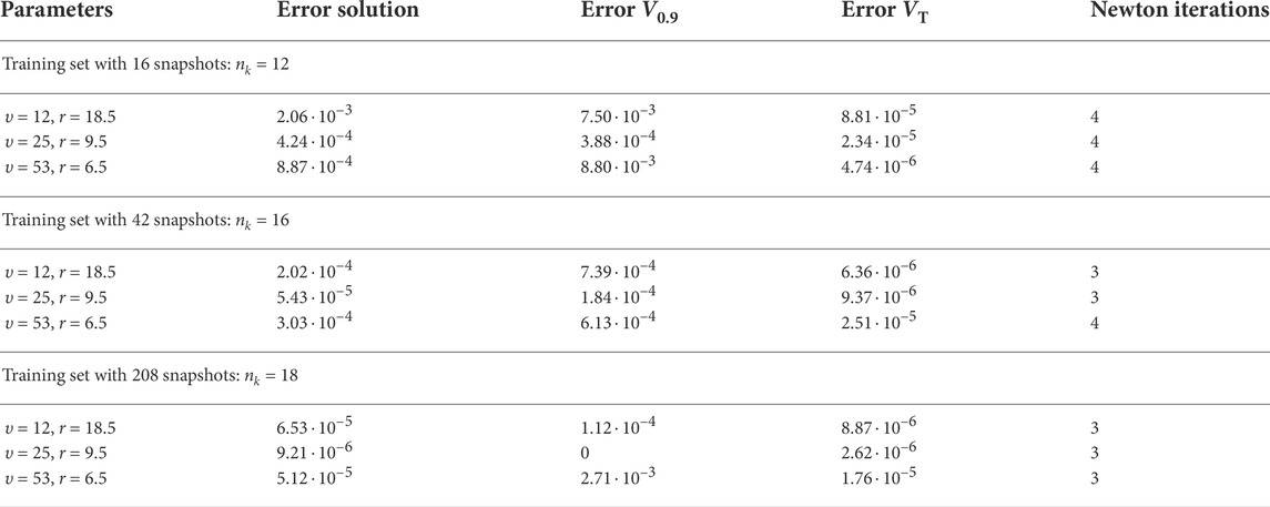
TABLE 1. Relative errors and number of Newton iterations of standard POD when solving the BVP in (Eq. 1). Training sets with 16, 42 and 208 snapshots are used to approximate solutions for parameters (υ, r) = (12, 18.5) (25, 9.5) and (53, 6.5). The truncation tolerance in POD is ɛ = 10^–3, and the tolerance for convergence in the Newton scheme is 10^–6.

The accuracy is remarkable in all cases given the number of snapshots. Also, note that the number of Newton iterations needed to converge is below five in all cases. These results validate the suitability of POD to solve the forward problem.

3.2 Performance of the hyper-reduction strategy

Next, we use the hyper-reduction strategy presented in Section 2.2.2 to assemble the system in the POD formulation. We consider the intermediate training set with 42 snapshots, reducing the number of degrees of freedom to n_k = 16.

Test 1: Hyper-reduction of (only) the matrix

The first test consists in hyper-reducing only the Jacobian in the Newton formulation, while keeping the standard POD assembly and projection of the residual. This is, we approximate the nonlinear dependences on c^k in matrix K(c^k; μ) with the hyper-reduction strategy based on tranining sets Y and G, but the full-order vector f(c^k; μ) is assembled at every iteration of the Newton scheme.

The accuracy of the hyper-reduced formulation is compared with that of standard POD in Table 2 for the previous parametric points (v, r) = (12, 18.5), (25, 9.5) and (53, 6.5). We take different truncation tolerances in the matrix approximations (Eq. 34) and (Eq. 35). We consider the approximation of A₁ and A₂ given by only their evaluation on the means $\bar{\mathit{y}}$ and $\bar{\mathit{g}}$, this is, ${\mathit{A}}_1({\mathit{c}}^k)\simeq {\mathit{A}}_1^{\mathit{red}}(\bar{\mathit{y}})$ and ${\mathit{A}}_2({\mathit{c}}^k)\simeq {\mathit{A}}_2^{\mathit{red}}(\bar{\mathit{g}})$ (n_kY = n_kG = 0). Also, we truncate the approximation with tolerances ɛ_K = 10^–1 and ɛ_K = 10^–3 for both training sets Y and G. With ɛ_K = 10^–1 the number of terms in the approximations are n_kY = 3 and n_kG = 4. By decreasing the tolerance to ɛ_K = 10^–3, the number of terms increases to n_kY = 14 and n_kG = 17.

TABLE 2

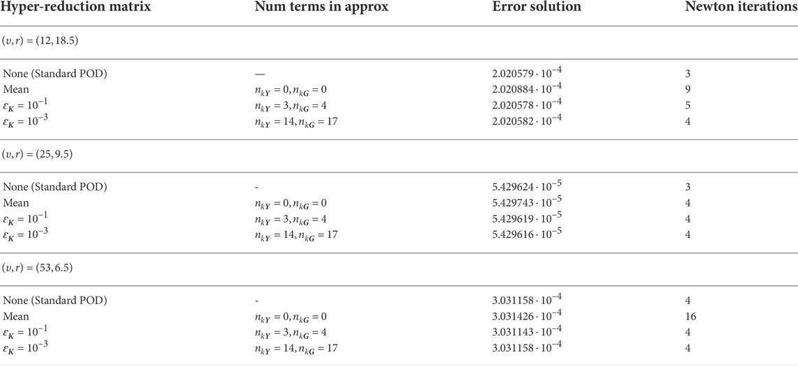
TABLE 2. Relative errors and number of Newton iterations when approximating only the matrix in the POD formulation with hyper-reduction. The hyper-reduction takes n_kY and n_kG terms in approximations (Eq. 34) and (Eq. 35) for A₁ and A₂, respectively. Solutions corresponding to parameters (υ, r) = (12, 18.5), (25, 9.5) and (53, 6.5). Training set with 42 snapshots, which leads to reduced systems of dimension n_k = 16.

Note that all options lead to the same relative error in the reduced-order solution up to (at least) 7 decimals. Indeed, the accuracy of the solution is dictated by the residual of the system, which here is computed with the standard POD approach. The number of iterations needed to converge increases for rough approximations of the matrix. In particular, we observe the highest number of iterations when the matrix is approximated by its mean. However, we remark that in this case the scheme less computationally demanding.

Indeed, for n_kY > 0 and n_kG > 0, the coefficients in the linear combination of terms are updated as the solution of the Newton scheme is modified. The computational expense of assembling a full-order matrix at every iteration is replaced by the computation of y^k = y (c^k) and g^k = g (c^k) and the linear combination of precomputed n_k × n_k matrices. Contrarily, approximating the matrices for their evalution on the means implies taking a constant matrix for all iterations k of the Newton scheme, with no additional computations.

Test 2: Hyper-reduction of the vector

From the previous test, we deduce that the hyper-reduced approximation of the matrix is robust in terms of accuracy. Next, we study the effect of applying the hyper-reduction strategy to the right-hand side vector, approximating the contribution of ${\mathit{f}}_1^{\mathit{red}}({\mathit{g}}^k)$ by (Eq. 40).

Approximating the residual is more critical since we may converge to a different solution. Accuracy is then affected by both the POD approximation of the solution and the approximation of the residual. Table 3 lists the errors and the number of Newton iterations for the previous parametric points, when using standard POD and for the hyper-reduced residual formulation with tolerance ɛ_f = 10^–3. For the matrix, we consider its approximation using the mean values ${\mathit{A}}_1({\mathit{c}}^k)\simeq {\mathit{A}}_1^{\mathit{red}}(\bar{\mathit{y}})$ and ${\mathit{A}}_2({\mathit{c}}^k)\simeq {\mathit{A}}_2^{\mathit{red}}(\bar{\mathit{g}})$, as well as the hyper-reduction with tolerance ɛ_K = 10^–3.

TABLE 3

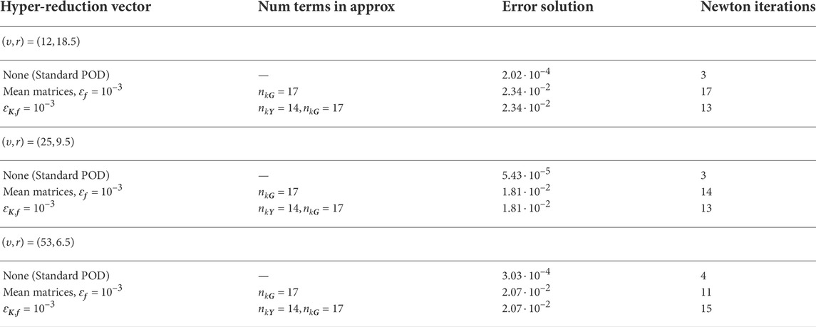
TABLE 3. Relative errors and number of Newton iterations when approximating the matrix and the vector in the POD formulation with hyper-reduction, with tolerance ɛ_f for the vector and mean matrices, and tolerance ɛ_K,f for approximating both the matrix and the vector. Solutions corresponding to parameters (υ, r) = (12, 18.5) (25, 9.5) and (53, 6.5). Training set with 42 snapshots.

We observe again that the accuracy of the reduced-order solution is determined by the approximation of the residual. With the same tolerance ɛ_f, we obtain the same relative error for both approximations of the matrix. As expected, errors increase when approximating the residual: for standard POD errors are of the order of 10^–4, while errors from the hyper-reduced formulation are of the order of 10^–2. The number of Newton iterations also increases, being below 20 in all cases. However, it is worth mentioning that we avoid assembling the full-order matrices and vectors, which is beneficial in terms of efficiency.

3.3 Inverse problem: Parameter identification

We define V* as the observables computed from the full-order FE solution for parameters υ = 35 and r = 12.5. We aim at recovering an approximation for the parameters, υ^⋆ and r^⋆, by solving the corresponding inverse problem (Eq. 13). In order to minimize the discrepancy functional $\mathcal{J}(\upsilon ,r)$ (Eq. 12), we evaluate it on a 50 × 50 grid on the parametric space I_υ × I_r using the hyper-reduced formulation for the training set with 42 snapshots.

In the Fenics implementation, assembling and projecting the residual of the system is very efficient. Thus, in our case, the most suitable option is to hyper-reduce the matrix, approximating the nonlinear dependences on c^k by their evaluation on the means $\bar{\mathit{y}}$ and $\bar{\mathit{g}}$, and to fully assemble the vector at every iteration of the Newton scheme to avoid losing accuracy.

Figure 2A shows the value of the functional $\mathcal{J}(\upsilon ,r)$ on the 50, ×, 50 parametric discretization. In this case, the minimization finds υ* = 35.9184 and r* = 12.9592, which are not the best possible approximations for the given discretization. We observe that there is a relation between the two parameters: there are different combinations that lead to a small value of the discrepancy functional. Actually, in Figure 2B, we mark the points for which $\mathcal{J}(\upsilon ,r)/\max (\mathcal{J})<10^{-2}$. This indicates the ill-posedness of the simultaneous minimization over parameters υ and r.

FIGURE 2

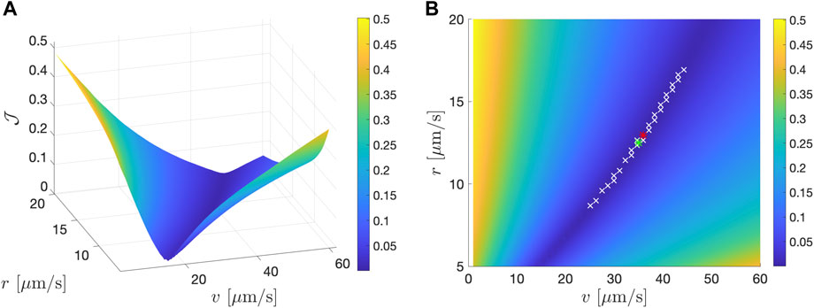
FIGURE 2. (A) Discrepancy functional $\mathcal{J}(\upsilon ,r)$ evaluated on a 50 × 50 grid on the parametric space I_υ × I_r. (B) White crosses indicate the points for which $\mathcal{J}(\upsilon ,r)/\max (\mathcal{J})<10^{-2}$. The obtained minimum (in red) is not he best possible approximation for (υ, r) = (35, 12.5) (in green).

We repeat the process by minimizing with respect to each one of the parameters separately. First, we fix r = 12.5 and discretize I_υ with 50 equispaced points. The value of the functional with respect to υ is plotted in Figure 3A. In this case, the minimization problem is well-defined, and leads to the opitmal υ* = 34.7143. Setting υ = 35 and discretizing for r, the minimum is also optimal, r* = 12.6531, Figure 3B.

FIGURE 3

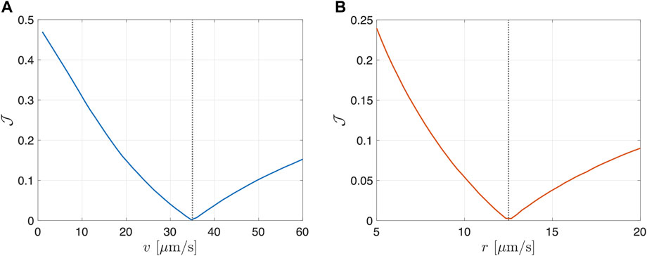
FIGURE 3. (A) Discrepancy functional $\mathcal{J}(\upsilon ,r)$ evaluated on a 50-point discretization of I_υ for r = 12.5. (B) Discrepancy functional $\mathcal{J}(\upsilon ,r)$ evaluated on a 50-point discretization of I_r for υ = 35.

4 Discussion and conclusion

We solve the inverse problem associated to the Ca²⁺ concentration in the intersitital fluid across a realistic 3D-printed structured scaffold. Given the values of some observables that characterize the expected bone formation, we aim at recovering the value of two parameters: the velocity amplitude, υ, and the ionic release rate from the scaffold, r.

The nonlinearity of the model and the multiple evaluations required to solve the inverse problem motivate the definition of a ROM strategy. We combine POD, to reduce the number of degrees of freedom, with a novel adhoc hyper-reduction strategy to accelerate the assembly of the full-order system at every iteration of the Newton method. The hyper-reduction is based on the PCA reduction of two additional training sets, which are derived from the weak form of the problem at hand. The idea is to approximate the nonlinear contributions in the matrices and vectors in the Newton scheme by linear combinations of precomputed matrices and vectors of reduced dimension. The formulation is exclusive for this problem, but it can be easily extended to other nonlinear problems with a suitable definition of the training sets. This strategy is applicable in cases in which the nonlinearity is explicitly described in the equations.

From the numerical tests, we conclude that the accuracy of the reduced-order solution is only dictated by the hyper-reduction of the vector of the system. For a fixed approximation of the residual, we obtain the same accuracy independently of the number of terms in the approximation of the Jacobian. In particular, replacing the nonlinear contributions of the matrix by their evaluation on the mean of the training sets is a competitive option in terms of accuracy and efficiency. The hyper-reduction of the matrix increases the number of Newton iterations needed to converge, but it still implies a gain in efficiency since the assembly of the full-order system is avoided. The hyper-reduction of the residual is more critical since it affects the accuracy of the reduced-order solution. However, we still obtain reasonable errors below 5%.

The solution of the inverse problem indicates a relation between the two parameters, υ and r. In order to obtain a well-posed minimization problem, we need to fix one of them and minimize with respect to the other. However, from a practical point of view, obtaining a relation between the parameters (instead of some unique values) that lead to the desired observables is also of interest.

Data availability statement

The raw data supporting the conclusion of this article will be made available by the authors, without undue reservation.

Author contributions

AM, SZ, AG-G, and PD worked on the conceptualisation, methodology and formal analysis. AM and AG-G worked on the investigation. AM wrote the draft of the manuscript. AG-G, SZ, and PD contributed to project supervision, manuscript revision, read and approved submitted version.

Funding

The authors acknowledge the financial support from the Ministerio de Ciencia e Innovación (MCIN/AEI/10.13039/501100011033) through the grants PID2020-113463RB-C32, PID2020-113463RB-C33 and CEX2018-000797-S.

Conflict of interest

The authors declare that the research was conducted in the absence of any commercial or financial relationships that could be construed as a potential conflict of interest.

Publisher’s note

All claims expressed in this article are solely those of the authors and do not necessarily represent those of their affiliated organizations, or those of the publisher, the editors and the reviewers. Any product that may be evaluated in this article, or claim that may be made by its manufacturer, is not guaranteed or endorsed by the publisher.

References

Alnaes, M. S., Blechta, J., Hake, J., Johansson, A., Kehlet, B., Logg, A., et al. (2015). The FEniCS project version 1.5. Arch. Numer. Softw. 3. doi:10.11588/ans.2015.100.20553

CrossRef Full Text | Google Scholar

Barba, A., Diez-Escudero, A., Maazouz, Y., Rappe, K., Espanol, M., Montufar, E. B., et al. (2017). Osteoinduction by foamed and 3D-printed calcium phosphate scaffolds: effect of nanostructure and pore architecture. ACS Appl. Mater. Interfaces 9, 41722–41736. doi:10.1021/acsami.7b14175

PubMed Abstract | CrossRef Full Text | Google Scholar

Berkooz, G., Holmes, P., and Lumley, J. L. (1993). The proper orthogonal decomposition in the analysis of turbulent flows. Annu. Rev. Fluid Mech. 25, 539–575. doi:10.1146/annurev.fl.25.010193.002543

CrossRef Full Text | Google Scholar

Bohner, M., Maazouz, Y., Ginebra, M.-P., Habibovic, P., Schoenecker, J., Seeherman, H., et al. (2022). Sustained local ionic homeostatic imbalance (SLIHI) caused by calcification modulates inflammation to trigger ectopic bone formation. Acta Biomater. 145, 1–24. doi:10.1016/j.actbio.2022.03.057

PubMed Abstract | CrossRef Full Text | Google Scholar

Chaturantabut, S., and Sorensen, D. (2010). Nonlinear model reduction via discrete empirical interpolation. SIAM J. Sci. Comput. 32, 2737–2764. doi:10.1137/090766498

CrossRef Full Text | Google Scholar

Danoux, C., Bassett, D., Othman, Z., Rodrigues, A., Reis, R., Barralet, J., et al. (2015). Elucidating the individual effects of calcium and phosphate ions on hmscs by using composite materials. Acta Biomater. 17, 1–15. doi:10.1016/j.actbio.2015.02.003

PubMed Abstract | CrossRef Full Text | Google Scholar

Díez, P., Muixí, A., Zlotnik, S., and García-González, A. (2021). Nonlinear dimensionality reduction for parametric problems: a kernel proper orthogonal decomposition. Int. J. Numer. Methods Eng. 122, 7306–7327. doi:10.1002/nme.6831

CrossRef Full Text | Google Scholar

Guyot, Y., Papantoniou, I., Chai, Y. C., Van Bael, S., Schrooten, J., Geris, L., et al. (2014). A computational model for cell/ECM growth on 3D surfaces using the level set method: a bone tissue engineering case study. Biomech. Model. Mechanobiol. 13, 1361–1371. doi:10.1007/s10237-014-0577-5

PubMed Abstract | CrossRef Full Text | Google Scholar

Habraken, W., Habibovic, P., Epple, M., and Bohner, M. (2016). Calcium phosphates in biomedical applications: materials for the future? Mater. Today 19, 69–87. doi:10.1016/j.mattod.2015.10.008

CrossRef Full Text | Google Scholar

Késmárky, G., Kenyeres, P., Rábai, M., and Tóth, K. (2008). Plasma viscosity: a forgotten variable. Clin. Hemorheol. Microcirc. 39, 243–246. doi:10.3233/CH-2008-1088

PubMed Abstract | CrossRef Full Text | Google Scholar

Langtangen, H. P., and Logg, A. (2017). Solving PDEs in Python. The FEniCS tutorial. Springer. doi:10.1007/978-3-319-52462-7

CrossRef Full Text | Google Scholar

Manhas, V., Guyot, Y., Kerckhofs, G., Chai, Y. C., and Geris, L. (2017). Computational modelling of local calcium ions release from calcium phosphate-based scaffolds. Biomech. Model. Mechanobiol. 16, 425–438. doi:10.1007/s10237-016-0827-9

PubMed Abstract | CrossRef Full Text | Google Scholar

Muixí, A., Zlotnik, S., Calvet, P., Espanol, M., Lodoso-Torrecilla, I., Ginebra, M.-P., et al. (2022). A multiparametric advection-diffusion reduced-order model for molecular transport in scaffolds for osteoinduction. Biomech. Model. Mechanobiol. 21, 1099–1115. doi:10.1007/s10237-022-01577-2

PubMed Abstract | CrossRef Full Text | Google Scholar

Negri, F., Manzoni, A., and Amsallem, D. (2015). Efficient model reduction of parametrized systems by matrix discrete empirical interpolation. J. Comput. Phys. 303, 431–454. doi:10.1016/j.jcp.2015.09.046

CrossRef Full Text | Google Scholar

Nguyen, N., and Peraire, J. (2008). An efficient reduced-order modeling approach for non-linear parametrized partial differential equations. Int. J. Numer. Methods Eng. 76, 27–55. doi:10.1002/nme.2309

CrossRef Full Text | Google Scholar

Patera, A. T., and Rozza, G. (2007). Reduced basis approximation and A-posteriori error estimation for parametrized partial differential equations. Cambridge, MA, USA: MIT Pappalardo Graduate Monographs in Mechanical Engineering, Massachusetts Institute of Technology.

Google Scholar

Quarteroni, A., and Rozza, G. (2014). Reduced order methods for modeling and computational reduction, 9. Springer. doi:10.1007/978-3-319-02090-7

CrossRef Full Text | Google Scholar

Ripamonti, U., Richter, P. W., and Thomas, M. E. (2007). Self-inducing shape memory geometric cues embedded within smart hydroxyapatite-based biomimetic matrices. Plastic Reconstr. Surg. 120, 1796–1807. doi:10.1097/01.prs.0000287133.43718.89

PubMed Abstract | CrossRef Full Text | Google Scholar

Santamaría, V. A. A., Malvè, M., Duizabo, A., Tobar, A. M., Ferrer, G. G., Aznar, J. G., et al. (2013). Computational methodology to determine fluid related parameters of non regular three-dimensional scaffolds. Ann. Biomed. Eng. 41, 2367–2380. doi:10.1007/s10439-013-0849-8

CrossRef Full Text | Google Scholar

Tang, Z., Li, X., Tan, Y., Fan, H., and Zhang, X. (2018). The material and biological characteristics of osteoinductive calcium phosphate ceramics. Regen. Biomater. 5, 43–59. doi:10.1093/rb/rbx024

PubMed Abstract | CrossRef Full Text | Google Scholar

Van hede, D., Liang, B., Anania, S., Barzegari, M., Verlée, B., Nolens, G., et al. (2021). 3D-printed synthetic hydroxyapatite scaffold with in silico optimized macrostructure enhances bone formation in vivo. Adv. Funct. Mater. 32, 2105002. doi:10.1002/adfm.202105002

CrossRef Full Text | Google Scholar