Error Analysis in Numerical Simulation of the Static Pressure Capability of Magnetic Fluid Seals

Magnetic fluid is a typical type of functional fluid which can be magnetized and controlled by an external magnetic field. In magnetic fluid seals, magnetic fluid is attracted in sealing gaps by a magnetic field gradient to form non-contact sealing. Compared to traditional sealing methods, they possess unique advantages such as zero leakage, long lifetime, low friction torque, and high reliability. Although the design and performance estimation of magnetic fluid seals rely mostly on numerical simulation, a number of simplifications or even mistakes during the simulation process exist in previous studies. The error caused by simplifications and mistakes has not been studied, leading to a possible problem of simulation results in reliability and consistency with experimental data. Here, we examined the influence of common simplifications and mistakes in numerical simulation of the static pressure capability of magnetic fluid seals, including material properties, geometric modeling, and theoretical formulas. A novel method of structure optimization based on a derivative-free multiparameter algorithm is also presented. A test bench for magnetic fluid seals is established, and the difference between simulation and experimental results is discussed. This research provides a precise, efficient, and standard procedure for numerical simulation of magnetic fluid seals.

1 Introduction

Magnetic fluid is a typical type of magneto-sensitive functional material, which contains magnetic nanoparticles, surfactants, and carrier fluid. To enhance stability, magnetic nanoparticles (usually 10–100 nm) are coated with proper surfactants before they are dispersed in a carrier fluid. Magnetic fluid can be magnetized and controlled by an external magnetic field. Its response and tunable characteristics including rheological, morphological, thermal, and optical properties have become a research focus recently (Zhao et al., 2014; Afifah et al., 2016; Chen et al., 2021). Due to its unique and controllable properties, magnetic fluid has been widely applied in fields such as cancer treatment (Kozissnik et al., 2013), high accuracy sensors (Alberto et al., 2018), dampers (Li and Gong, 2019), water purification (Yang et al., 2019), and so on (Huang et al., 2021).

Among them, magnetic fluid seals (MFSs) are one of the most mature applications. In an MFS, magnetic fluid is attracted in sealing gaps by a magnetic field gradient to resist a pressure difference. As a non-contact sealing technology, it possesses unique advantages including zero leakage, long lifetime, low friction torque, and high reliability (Li, 2010). Therefore, it is suitable for high-demand sealing conditions such as rotary blood pumps (Mitamura et al., 2008), robot joints (Yang et al., 2018), and silicon crystal growing furnaces (Zahn, 2001), especially with a requirement of vacuum environment and a long maintenance cycle.

Numerical simulation is a necessary procedure during the design and performance estimation of MFSs. Generally, the finite element method (FEM) is used to obtain the magnetic field distribution. The static pressure capability of an MFS depends on the magnetization intensity of applied magnetic fluid and the gradient of magnetic field intensity in sealing gaps. However, it is practically impossible to measure the magnetic field intensity experimentally, because the sealing gaps are usually smaller than 0.2 mm, far narrower than the thickness of the smallest Hall sensor available (about 1 mm) (Szczech and Horak, 2017). Meanwhile, to realize the largest pressure capability with a limited axial length and sealing part volume, it is essential to optimize the geometric structure and predict the pressure capability during the design process. Kim et al. (2010) designed an MFS for underwater robotic vehicles by FEM, and conducted sealing experiments as a comparison. The difference in the static pressure capability between simulation and experiments is 9.3%, and the largest difference 33.5% occurs at a rotary speed of 400 rpm. Yang et al. (2013) proposed an MFS structure with multiple magnetic sources to improve pressure capability for sealing gaps larger than 0.25 mm. The simulation result was in good consistency with experiments when gaps were 0.4 mm, but the difference increased with the increase of sealing gaps. The difference was up to 36.0% when gaps were 0.7 mm. Szczęch (2020) studied the influence of pole tooth shapes and magnetic fluid volume on the difference, as well as the pressure transfer mechanism among stages. He found that the difference was mainly due to the simplification in determining the magnetic fluid–free surface, and errors accumulated from individual stages. Cong et al. (2012) designed a twin-shaft MFSs for wafer-handling robots, and optimized the geometric dimensions in numerical simulation by varying sealing gaps, tooth width, slot width, tooth height, and thickness of the shaft in turn. Parmar et al. (2021) realized the optimization of design parameters using mass data generated by FEM simulation and then multivariate regression analysis.

In summary, previous studies have provided a general numerical simulation of pressure capability during the design of various MFS structures, and extended MFSs to many engineering applications. However, the difference between simulation results and experimental data has always been a problem for researchers. The influence of simplifications and mistakes on the simulation error has not been thoroughly studied yet. A precise and standard procedure for numerical simulation of MFSs still needs to be proposed. Moreover, most researchers optimized the geometric structures of MFSs by varying different parameters in turn, which was inefficient and neglected the complex joint influence of those parameters.

In this research, the source of errors in numerical simulation of the static pressure capability of MFSs is examined. The influence of common simplifications and mistakes in existing studies is analyzed, including material properties, geometric modeling, and theoretical formulas. A standard procedure for FEM simulation of MFSs is proposed. Furthermore, a novel method of geometric parameter optimization based on a derivative-free multiparameter optimization algorithm is put forward. Finally, a test bench for MFSs is established and sealing experiments are conducted. Differences between improved numerical simulation and experimental results are discussed.

2 Material and Structure

Magnetic properties of magnetic fluid have a direct influence on the pressure capability of MFSs, and are key properties in the definition of materials in numerical simulation. Here, we take two types of magnetic fluid prepared in our laboratory as examples, MF-1 and MF-2. The relationship between the applied magnetic field and magnetization of magnetic fluid (M-H curves) shown in Figure 1 was measured using a vibrating sample magnetometer (VSM, LDJ Model 9600) at 20 °C. Important physical and magnetic properties are listed in Table 1. The coercivity of these two types of magnetic fluid is low enough, so they can be regarded as superparamagnetic materials. Therefore, a single-valued relationship exists between magnetization M and magnetic field intensity H, and between magnetic induction B and magnetic field intensity H. MF-1 is taken as an example in the demonstration of the following simulation, while both types are used in sealing experiments.

FIGURE 1

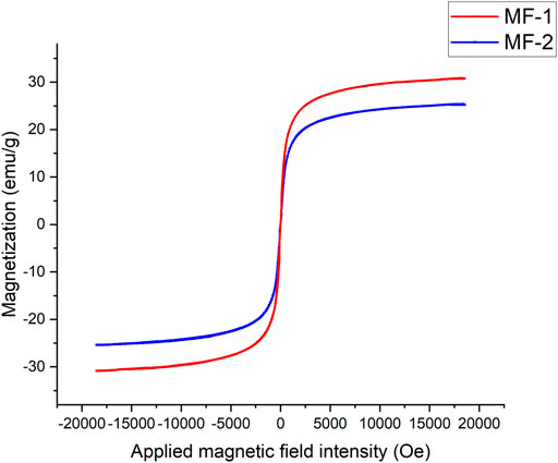
FIGURE 1. M–H curves of MF-1 and MF-2.

TABLE 1

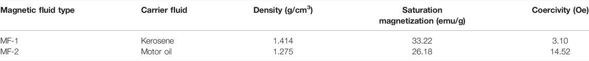
TABLE 1. Physical and magnetic properties of MF-1 and MF-2.

Figure 2 shows the schematic diagram of a typical MFS structure. The components to form a closed magnetic circuit are colored in the figure. The red loop indicates that the magnetic flux travels from the north pole of the magnet, through the pole piece, magnet fluid, the shaft, and the other pole piece, and finally ends at the south pole. Sleeves made of magnetically non-conductive materials are placed between pole pieces and bearings, so that the magnet does not affect the performance of bearings. Pole teeth are placed annularly at the end of the pole pieces. A strong magnetic field gradient exists in the sealing gaps between pole teeth and the shaft. As a result, magnetic fluid is attracted there by the magnetic force to resist a pressure difference, forming eight sealing stages. There are several commonly used shapes of pole teeth, such as triangular, rectangular, single-side trapezoidal, and isosceles trapezoidal (Parmar et al., 2018). Here, we focus on isosceles trapezoidal pole teeth.

FIGURE 2

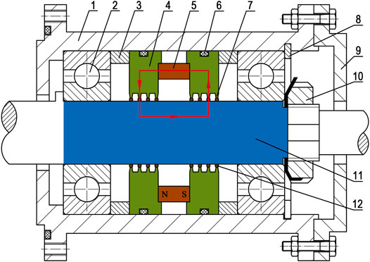
FIGURE 2. Schematic representation of a typical MFS structure (1-shell, 2-bearing, 3-sleeve, 4-pole piece, 5-magnet, 6-rubber ring, 7-pole tooth, 8-elastic collar, 9-end cover, 10-round nut, 11-shaft, and 12-magnetic fluid).

3 Theoretical Basis

The pressure capability of MFSs is derived based on the Bernoulli equation of magnetic fluid. This equation takes mechanical and magnetic energy into consideration, and is the foundation of industrial applications of magnetic fluid. For incompressible Newtonian steady-state liquid, for collinear and temperature-independent magnetization and in an irrotational flow field, the Bernoulli equation of magnetic fluid is (Rosensweig, 2013)

$p+\frac{1}{2}{\rho }_f{v}^2+{\rho }_{f}gh-{\mu }_0{\displaystyle {\int }_0^{H}MdH}=C,(1)$

where p, ρ_f, and v are the pressure, density, and velocity of magnetic fluid, respectively. g is the gravitational acceleration, h is the height of magnetic fluid, μ₀ is vacuum permeability, M is the magnetization intensity, H is the magnetic field intensity, and C is a constant. For a static MFS, if the gravity of magnetic fluid is negligible compared to the magnetic force, and the boundary of fluid coincides with the contour line of the magnetic field intensity approximately, then

$p_1-{\mu }_0{\displaystyle {\int }_0^{H_1}MdH}=p_2-{\mu }_0{\displaystyle {\int }_0^{H_2}MdH},(2)$

$\text{Δ}p=p_1-p_2={\mu }_0{\displaystyle {\int }_{H_1}^{H_2}MdH},(3)$

where p₁, p₂, H₁, and H₂ are the pressure and magnetic field intensity on two sides of magnetic fluid, respectively. The maximum pressure capability △p_max occurs when

$\text{Δ}{p}_{\max }={\mu }_0{\displaystyle {\int }_{H_{\min }}^{H_{\max }}MdH},(4)$

$\text{Δ}{p}_{\max }\approx {\mu }_0{M}_s\left(H_{\max }-H_{\min }\right),(5)$

where M_s is the saturation magnetization of magnetic fluid, H_max and H_min are the maximum and minimum magnetic field intensity in the sealing gap, respectively. The approximation in Eq. 5 is under the assumption that the magnetic field intensity is strong enough for magnetic fluid to reach saturation magnetization. The error will be discussed later. The total pressure capability of an MFS is calculated as the sum of each pole tooth.

4 Methods

4.1 General Procedure of Numerical Simulation

Magnetic field simulation of MFSs is usually performed by the finite element method, which divides the entire system into discrete meshes, establishes algebraic equations of each domain, assembles them into a larger system of equations and solves it (Cendes et al., 1983). A general procedure of numerical simulation of MFSs includes the modeling of geometric structures, definition of material properties, definition of magnetization and boundary conditions, meshing, calculation, and post-processing.

During the simulation process, several assumptions are followed. First, the magnet is magnetized uniformly axially, and the magnetic properties of other parts are axisymmetric. Therefore, the 3D structure can be reduced to a 2D axisymmetric model. Second, those parts made of magnetically non-conductive materials, such as aluminum alloy and stainless steel, have permeability equal to vacuum. So only magnetically conductive parts are modeled. Third, the dimensional error by manufacturing and assembly is neglectable, and the width of sealing gaps is uniform and constant as designed. The materials are defined to match the actual experimental situation, where the magnet is NdFeB grade N35, and the shaft and pole pieces are made of low carbon steel 45#. The magnetization characteristics are defined by their B–H curves. The axisymmetric condition is applied on the axis of symmetry, and the magnetic insulation condition is applied on the air boundaries. The initial magnetic scalar potential of the whole field is zero. The minimum meshing number in sealing gaps is 10.

4.2 Magnetic Property of Magnetic Fluid

The magnetic property of magnetic fluid is a key factor to determine the pressure capability. However, the influence of magnetic fluid on the magnetic field intensity is often ignored. Because the relative permeability of magnetic fluid is close to 1, the region of magnetic fluid is usually simplified as the air. This simplification brings apparent convenience to the modeling of the sealing structure, but when the magnetic field intensity is low, the permeability of magnetic fluid is significantly different from the air. As a result, for MFSs of a large sealing gap or weak magnetic sources, the error is magnified.

The error in the magnetic field intensity caused by the magnetic fluid can be solved by defining the B–H relationship of magnetic fluid during the simulation. The relationship can be derived from the experimental data of the VSM. However, because VSM measurements are an open-circuit process, the demagnetization effect must be taken into consideration. (Pugh et al., 2011). The magnetic induction B is calculated by

$B={\mu }_0\left(H_{in}+M\right)={\mu }_0\left(H_a+H_d+M\right)={\mu }_0\left(H_a+\left(1-N\right)\cdot M\right),(6)$

where H_in, H_a, and H_d are the internal, applied, and demagnetizing magnetic field intensity, respectively; N is the demagnetizing factor. The demagnetizing factor depends on the geometry and permeability of the sample. For cylindrical samples, former research (Chen et al., 1991) has provided a precise estimation of magnetometric demagnetizing factors of different ratios of length to diameter. Therefore, with the geometric dimensions of the cylindrical sample box used in VSM, the true relationship between B and H can be obtained by Eq. 6. To study the influence of magnetic fluid on the magnetic field intensity in sealing gaps, the areas occupied by the magnetic fluid under pole teeth are defined by the B–H relationship earlier.

4.3 Geometric Modeling

4.3.1 Air Domain

In former studies, a rectangular air domain is usually established to calculate the magnetic field in the surrounding region, as is shown in Figure 3A. But theoretically, magnetic energy is distributed in the whole field, and magnetic lines can extend to infinity. So a limited air domain will inevitably lead to an overestimated pressure capability of MFSs, due to the neglection of magnetic energy loss in the far field. On the other hand, the expansion of the air domain significantly increases the grid numbers and lowers the computational efficiency. Therefore, a proper dimension of the air domain needs to be defined, so that the exterior boundaries have little effect on the magnetic field intensity of the central working area, and the computing time is acceptable as well.

FIGURE 3

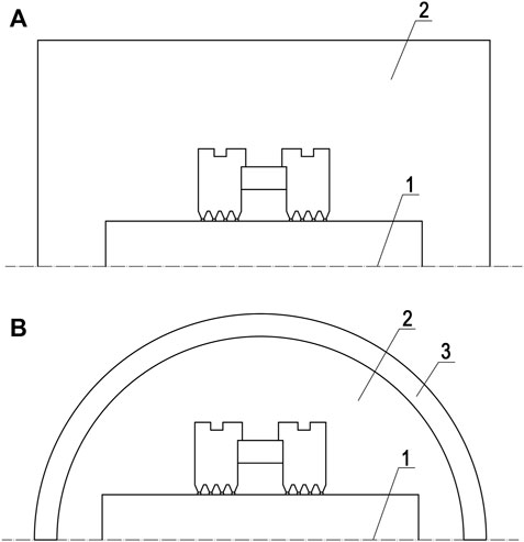
FIGURE 3. Geometric modeling of an MFS structure with (A) rectangular air domain (B) circular air domain with infinite elements (1-axis of symmetry, 2-air domain, and 3-infinite domain).

Furthermore, to realize better calculation accuracy and higher computing efficiency, infinite elements are employed in the geometric modeling of the air domain for the first time. In Figure 3B, region three is a layer of virtual domains which can be stretched out toward infinity. A semi-infinite coordinate stretching in the radial direction is applied to the infinite elements by a mapping function of a dimensionless coordinate, which changes from 0 to 1 in the infinite element layer (Jin, 2015). The function is usually rational, so that the infinite domain is extremely large compared to the geometry dimensions. By this means, the magnetic field solution of the central working area is not affected by the artificial boundaries.

4.3.2 Parallel Magnets

In engineering applications, especially when the diameter of the shaft is large, a single annular permanent magnet as the magnetic source is too difficult to manufacture or assemble. In these cases, several or even tens of cylindrical magnets are placed between adjacent pole pieces in parallel. The problem is that, a 3D model is more complex and computationally consuming than a 2D axisymmetric model of the same sealing structure. Therefore, this study aimed to find a reasonable simplification method of parallel magnets into a 2D model. The diameter-equivalent method indicates that the equivalent magnet in a 2D model has the same radial length as a 3D model, and the volume-equivalent method refers to the same volume as a 3D model. The errors of these two methods are then compared.

4.3.3 Magnetic Fluid Boundary

According to Eq. 2, if the surface tension of magnetic fluid is neglectable, then the boundaries of magnetic fluid are assumed to overlap the contour line of the magnetic field intensity. There are two possible sources of errors. First, because the boundaries of magnetic fluid at the critical position before a sealing failure occurs are complex to depict, former studies tend to simplify the boundaries as parts of a circle or ellipse, or even replace the magnetic fluid as the air. But the influence of dynamically changing boundaries of magnetic fluid on the magnetic field distribution, further on the pressure capability remains unfocused. Second, the minimum magnetic field intensity under each pole tooth is determined by the magnetic fluid boundary on the low-pressure side. As a result, the volume of magnetic fluid at each sealing stage is the main determinant of pressure capability. In this part, the precise boundaries of magnetic fluid overlapping the contour lines of the magnetic field intensity are calculated and depicted, and the magnetic field distribution is compared with simplified boundaries. The relationship between the volume of magnetic fluid and pressure capability is studied quantitatively.

4.4 Pressure Capability Formula

In previous studies (Zhang et al., 2019; Parmar et al., 2020) about MFSs, Eq. 5 is mostly adopted to evaluate the pressure capability. The popularity of this formula lies in its simple form, which divides the magnetic property of magnetic fluid M_s and magnetic field intensity difference H_max–H_min as two separate objects. The basic assumption here is that, the magnetic field intensity in sealing gaps is large enough for magnetic fluid to reach magnetic saturation. However, as is shown in Figure 4, the M–H curve of typical magnetic fluid can be divided into two zones, the unsaturated zone and saturated zone. In the unsaturated zone, as the magnetic field intensity increases, more domains inside the magnetic fluid reorientate and stay parallel with the magnetic field. After most domains have been reorientated, further increase in the magnetic field intensity only results in a minor change of magnetization.

FIGURE 4

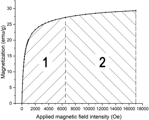
FIGURE 4. M–H curve of the typical magnetic fluid (1-unsaturated zone, 2-saturated zone).

As a result, the commonly used formula has two problems. First, when the sealing gap is large, or the magnetic source is not strong enough, part of the magnetic fluid is far from saturation. The pressure capability is overestimated consequently. Second, the saturation magnetization is only an estimated value, because the magnetization keeps elevating slowly but incessantly. Some former researchers tried to divide the curve into segments and calculate the area separately (Li, 2010). In this research, a more accurate and straightforward method is proposed, which calculates the integral of interpolation function of the M–H curve based on Eq. 4.

4.5 Structure Optimization

During the design and evaluation of an MFS structure, the optimization of geometric parameters of pole teeth is crucial. It determines the difference of magnetic field intensity in sealing gaps, and further the pressure capability. Former researchers (Cong et al., 2012; Szczęch et al., 2017) adopted a “one-by-one” method to optimize different parameters of pole teeth, which varies one parameter at a time. Taking rectangular pole teeth as an example, the width of pole teeth is first varied to find the largest pressure capability, with the height of pole teeth and interval between adjacent pole teeth fixed. Then, the optimized width is fixed and the other parameters are varied one by one. This optimization method ignores the joint influence on the pressure capability by different parameters. In other words, an optimal pole tooth height at a certain width may not be the optimal value at another width. So this method cannot acquire a global optimal variable set. Moreover, the efficiency gets poorer if more variables are considered during the design process.

Here, the coordinate descent method as a derivative-free multiparameter optimization algorithm is applied to optimize the geometric parameters of pole teeth. This is a class of optimization algorithms, where the optimization process is not based on the derivative of the objective function (Larson et al., 2019). It is especially appropriate for pole tooth design, because the relationship between pressure capability and structural parameters can hardly be solved analytically. By the coordinate descent method, starting with the control variable set at the start of kth iteration ${\mathit{x}}^{\left(k\right)}$, a finite number of points are searched along coordinate directions so that $f\left(\mathit{x}\right)<f\left({\mathit{x}}^{\left(k\right)}\right)$. If so, the new variable set is replaced as ${\mathit{x}}^{\left(k+1\right)}={\mathit{x}}^{\left(k\right)}$. Otherwise, points are evaluated from the poll set ${\mathit{P}}^{\left(k\right)}$.

${\mathit{P}}^{\left(\mathit{k}\right)}=\left\{{\mathit{x}}^{\left(\mathit{k}\right)}+{\alpha }_k\mathit{d}|\mathit{d}\in D_k\right\},(7)$

where α_k is the step size and D_k is a positive basis of the variable space. If a better point with a smaller objective value in the poll set is found so that $f\left({\mathit{x}}^{\left(k\right)}+{\alpha }_k{\mathit{d}}^{\left(k\right)}\right)<f\left({\mathit{x}}^{\left(k\right)}\right)$, then the variable set is updated. Otherwise, the variable set remains unchanged, and the step size is decreased. The optimization process ends when the step size is less than a prescribed limitation, or the maximum iteration number is reached. The optimization results obtained using the coordinate descent method and “one-by-one” method are compared and discussed.

4.6 Experimental Setup

To validate the improved numerical simulation method, a test bench for MFSs is established. Key components of the sealing prototype are shown in Figure 5, including a gas chamber, a shell with two bearings inside, a magnetically conductive inner sleeve, a shaft, a magnetic unit consisting of parallel magnets and two pole pieces, and an end cover. The pole pieces are assembled on the shaft instead of the shell, so that pole teeth are exposed for the ease of magnetic fluid injection. Two pairs of pole pieces are manufactured and used. One pair has one rectangular pole tooth per pole piece, with the width of pole teeth 1 mm and the height 2 mm. The other pair has five rectangular pole teeth per pole piece, with the width 0.5 mm, the height 2 mm, and the interval 2.5 mm. The sealing gap is 0.3 mm.

FIGURE 5

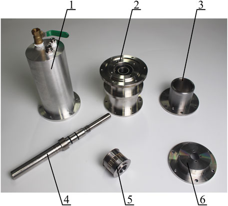
FIGURE 5. Key components of the sealing prototype (1-gas chamber, 2-shell with bearings inside, 3-inner sleeve, 4-shaft, 5-magnetic unit, and 6-end cover).

Figure 6 indicates the set-up of MFS experiments. In each sealing experiment, a certain amount of magnetic fluid is injected into each pole tooth, as is shown in Figure 7. Then, the shaft is pushed into the shell and fixed. The end cover is installed and the gas and electric circuits are connected. At the beginning, all valves are closed except for the air compressor. The outflow air is adjusted to a modest stable pressure (100 kPa for example). After that, the ball valve is turned on slowly and the air in the gas chamber is compressed. The pressure in the first and second stages of the MFS is collected by pressure sensors and written on the computer. Finally, a sudden pressure drop occurs, indicating the bursting of magnetic fluid and a sealing failure. The critical pressure before the failure is recorded as the pressure capability. For each different sealing condition, the experiments are repeated three times and the average value and standard deviation are calculated.

FIGURE 6

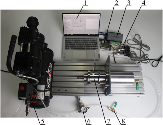
FIGURE 6. Test bench for MFSs (1-computer, 2-power supply, 3-data acquisition card, 4-pressure sensor, 5-air compressor, 6-regulator valve, 7-sealing prototype, and 8-ball valve).

FIGURE 7

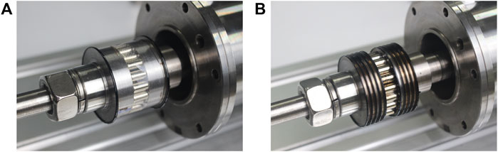
FIGURE 7. Magnetic fluid injection on pole teeth. (A) One pole tooth and (B) five pole teeth per pole piece.

5 Results and Discussion

5.1 Effect of the Magnetic Property of Magnetic Fluid

The ratio of length to diameter of the sample box is measured as 0.422, and the demagnetization factor along the magnetic field direction is 0.242 by interpolation. In Figure 8A, the M–H curve of MF-1 by different demagnetizing factors is plotted. After demagnetization correction, the magnetization is higher than original values, and the largest deviation exists in the unsaturated zone, where the magnetic field intensity is rather low. For the sample box used in the experiment, the demagnetization effect is not obvious.

FIGURE 8

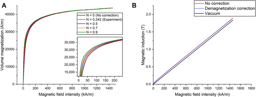
FIGURE 8. (A) M–H curve and (B) B–H curve of MF-1 with and without demagnetization correction.

As is shown in Figure 8B, the magnetic induction of magnetic fluid is higher than vacuum (or air), but the curves with and without the demagnetization correction are almost overlapped. The maximum difference caused by the demagnetization effect is lower than 1%. The main reason is the relatively low magnetization intensity of magnetic fluid. The pressure capability of magnetic fluid with and without the demagnetization correction and of air is 229.48, 229.04, and 232.86 kPa, respectively. Consequently, an error of 1.5% exists if magnetic fluid is simplified as air, but the influence of the demagnetization effect is negligible.

5.2 Effect of Geometric Modeling

5.2.1 Air Domain

For the traditional rectangular air domain, the width of the air domain is varied from 35 to 200 mm and the pressure capability is calculated, as is shown in Figure 9. The length of the air domain is twice the width. The total degrees of freedom are also depicted reflecting the computing complexity. As the air domain expands, the pressure capability decreases rapidly at first, and then converges to about 229.6 kPa. Meanwhile, the total degrees of freedom rise, indicating a larger computing amount due to more grids generated in the air domain. For this traditional air domain method, a balance between magnetic energy loss in the far field and computing efficiency needs to be considered, and five times the size of the working area is recommended in practice. In comparison, the simulation result by infinite elements is 229.63 kPa, and the total degree of freedom is 3.1×10⁵. By an infinite element layer, the error of energy loss the in the far field is significantly decreased, while the computing efficiency remains satisfactory. Infinite elements prove to be a better method to model the air domain.

FIGURE 9

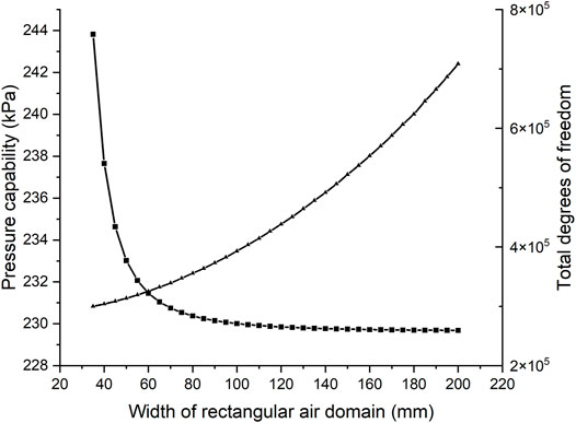
FIGURE 9. Pressure capability (block) and total degrees of freedom (triangle) with different widths of the rectangular air domain.

5.2.2 Parallel Magnets

For MFSs with parallel magnets, the number of magnets used in the device is determined by the requirement of pressure capability, the inner space, assembling difficulty, etc. In this case, different numbers of cylindrical magnets of 10 mm height and 5 mm diameter are simulated by 3D models. 3D simulation provides the most precise result evidently, but is not applicable practically due to the computing time as long as 100 times of 2D models. Therefore, 2D simulation with diameter-equivalent and volume-equivalent methods is conducted. The pressure capability of the former method is 229.48 kPa and the latter is shown in Table 2.

TABLE 2

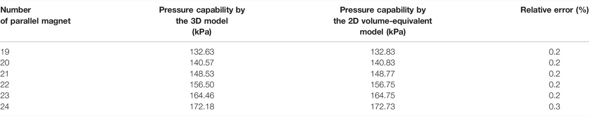
TABLE 2. Pressure capability of 3D and 2D volume-equivalent models with parallel magnets.

Numerical simulation indicates a significant influence on the pressure capability by the number or volume of magnets. The pressure capability increases linearly with the number of parallel magnets (linear correlation coefficient R = 0.99999), which has not been reported by previous studies. This indicates a relatively fixed magnetic energy provided by a certain volume of magnets. As a result, a large error exists between 3D simulation and 2D simulation with the diameter-equivalent method, and the error decreases with more magnets. The relative error from 3D simulation is 33.3% with 24 parallel magnets. It is mainly because the gaps between adjacent magnets cannot provide magnetic energy. Meanwhile, the volume-equivalent method shows a great consistency with the 3D model for different numbers of parallel magnets, which is preferred to simplify a 3D model with parallel magnets into a 2D axisymmetric one.

5.2.3 Magnetic Fluid Boundary

Three common descriptions of the magnetic fluid boundary are studied, including the contour line of magnetic field intensity, ellipses, and simplification as air. The maximum magnetic field intensity under three conditions is similar, and the largest difference is about 1%. Consequently, the magnetization of the magnetic fluid itself has little effect on the magnetic field distribution. The major influence of the magnetic fluid boundary is on the determination of minimum magnetic field intensity in Eq. 4, which is related to the volume of magnetic fluid under the pole tooth. Due to an uncertainty pattern of magnetic fluid distribution among multiple stages, here we take a single pole tooth per pole piece as an example.

Figure 10A demonstrates the magnetic fluid boundaries (calculated as contour lines of magnetic field intensity) at critical positions with different volumes. The black line on the left represents the boundary on the high pressure side, and part of it is deformed by the concentration of the magnetic field at the corner of pole teeth. In Figure 10B, the pressure capability increases with more magnetic fluid injected under the pole tooth. However, the increase is significant at first but then slows down. Also, the variation of pressure capability by the volume can be quite large. In conclusion, the influence of magnetic fluid boundaries lies in the determination of the minimum magnetic field intensity, and further the pressure capability. Although the theoretical volume is small, an excessive volume of magnetic fluid is usually injected in experiments. The resulting experimental errors are discussed later.

FIGURE 10

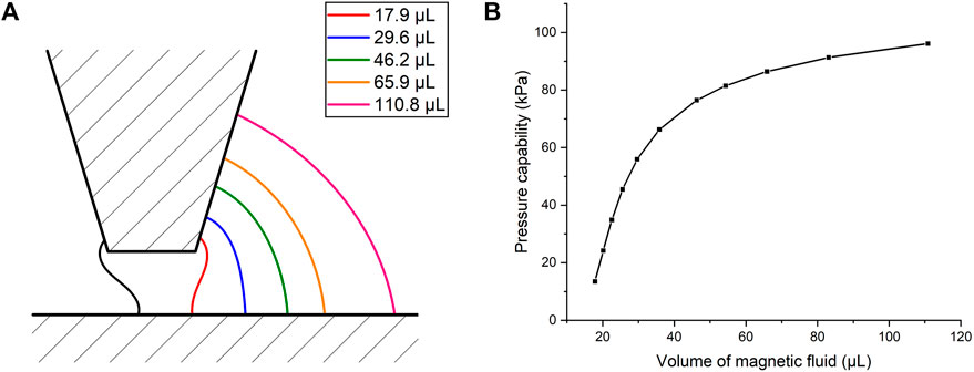
FIGURE 10. (A) Magnetic fluid boundaries at critical positions with different volumes. (B) Pressure capability varying with the volume of the magnetic fluid.

5.3 Effect of the Pressure Capability Formula

For the MFS simulation model presented earlier, Eq. 5 as the most adopted simplification of the pressure capability formula gives a result of 266.61 kPa, and the integral of interpolation function of the M–H curve based on Eq. 4 obtains 229.53 kPa. The error of 16.2% comes from the overestimation of saturation magnetization of magnetic fluid by the simplified formula, because in this case where the sealing gap is 0.3 mm, the magnetic field intensity in the sealing gaps is relatively low, and a large amount of magnetic fluid is far from saturation. In conclusion, the integral formula based on Eq. 4 is essential to decrease the simulation error, especially for large sealing gaps or a weak magnetic source.

5.4 Structure Optimization

For MFSs with isosceles trapezoidal pole teeth, four geometric parameters have a major influence on the magnetic field distribution, the width of pole teeth L_t, the height of pole teeth L_h, the angle of pole teeth α, and the interval between adjacent pole teeth L_m. Since the axial length of pole pieces is usually fixed, the first three parameters are independent control variables during the structure optimization, and the pressure capability is the objective function. The initial parameter set is selected as L_t = 0.8 mm, L_h = 1 mm and α = 55°.

Figure 11 shows the optimization process of the “one-by-one” method. Pressure capability with different widths of pole teeth is calculated, and the optimal width value is used in the next step. The optimization result of this method is 231.93 kPa, where the optimal variable set is L_t = 0.31 mm, L_h = 1.01 mm, and α = 71.0°. Meanwhile, the optimization result of the coordinate descent method is 244.64 kPa, with an iteration number of 183. The corresponding variable set is L_t = 0.45 mm, L_h = 1.81 mm, and α = 80.7°. Obviously, the multiparameter optimization obtains a 5.5% higher objective value than the traditional method. The main reason is the joint influence on pressure capability by different geometric parameters, as is demonstrated in Figure 12. This figure shows a stationary point in the variable set space, indicating the existence of a global optimal solution. However, the solution is not likely to be reached by variation of one control variable when the other variables remain fixed.

FIGURE 11

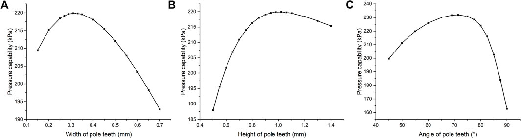
FIGURE 11. Pressure capability varying with (A) width, (B) height, and (C) angle of pole teeth.

FIGURE 12

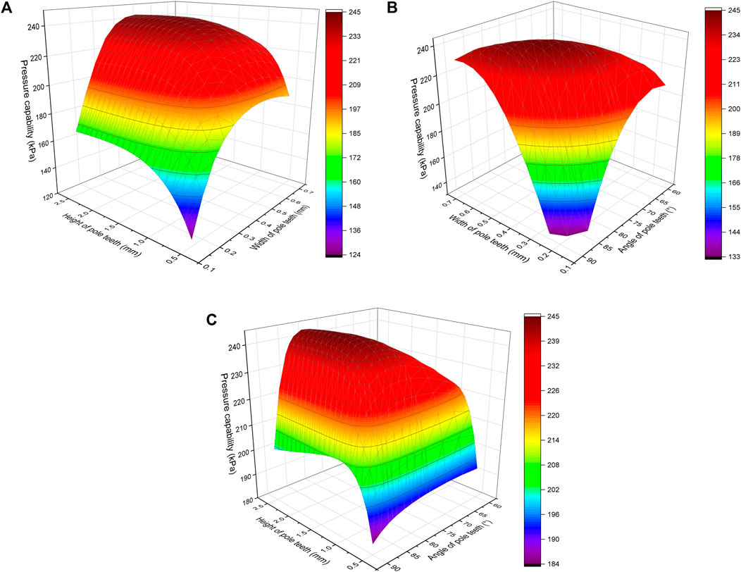
FIGURE 12. Joint influence on pressure capability by (A) width and height, (B) width and angle, and (C) height and angle.

To test the robustness of these two methods, another two initial variable sets are adopted. The first set is L_t = 0.5 mm, L_h = 2 mm, and α = 70°. The second set is L_t = 1 mm, L_h = 1.5 mm, and α = 90°. The “one-by-one” method leads to 241.66 and 236.30 kPa as maximum pressure capability, respectively. In comparison, the coordinate descent method obtains nearly the same result about 244.6 kPa at nearly the same variable set for all three conditions. Apparently, the multiparameter optimization algorithm is insensitive to initial values, and has higher design efficiency and a better optimization result compared to the traditional method.

5.5 Experimental Studies

MFS experiments with two types of magnetic fluid and two pairs of pole pieces are conducted. For each different sealing condition, the average value of pressure capability as well as standard deviation is calculated. The comparison between experimental and simulation results before and after improvement is shown in Table 3. For the unimproved simulation, the area of sealing gaps is simplified as air. The air domain is rectangular with 80 mm width and 160 mm length. The calculation of pressure capability is according to Eq. 5. For the improved simulation, the area occupied by the magnetic fluid under pole teeth is defined by the B–H relationship of magnetic fluid after demagnetization correction in Figure 8B. The air domain is circular with a radius of 70 mm and an 8 mm thick layer defined as infinite domains. The calculation of pressure capability is carried out by the integral of interpolation function of the M–H curve of magnetic fluid. Parallel magnets are both simplified with the volume-equivalent method. The improved simulation method reduces the errors to a large extent. The main reason is the integral of interpolation function of the M–H curve as the pressure capability formula in Section 4.4. The advantage and importance of this formula stand out, especially when the magnetic fluid is far from magnetic saturation, just like the sealing prototype. In addition, the application of infinite domains and proper simplification of magnets also enhance the calculation precision and efficiency.

TABLE 3

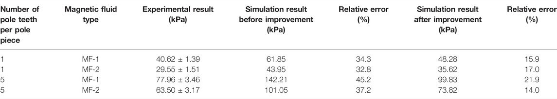
TABLE 3. Comparison between experimental and simulation results under different MFS conditions.

However, for both simulation methods, the errors of MFSs with five pole teeth per pole piece are generally higher than that of single pole tooth, which indicates a major problem of the current simulation. During the present simulation of multiple pole teeth, it is assumed that different sealing stages reach their maximum pressure capability at the same time, and they add up to the total pressure capability. But in fact, the mechanism of pressure transferring through stages is complex. The distribution of pressure among different pole teeth depends on the position of magnetic fluid, the compression process and even the sealing history, and remains unsolved theoretically. This leads to a general overestimation of pressure capability with multiple pole teeth compared to a single pole tooth.

In addition, the experimental setup and operation also account for part of the error. First, although a certain amount of magnetic fluid is injected into each pole tooth, redistribution and loss of magnetic fluid are likely to occur during the push-in process. Some magnetic fluid will be attracted near the magnets because of magnetic concentration. As a result, the actual volume remaining under pole teeth may be insufficient, and the pressure capability will decrease. Second, the sealing gap is not always uniform as 0.3 mm circularly, so the bursting of magnetic fluid tends to occur where the sealing gap is larger. The dimensional error by manufacturing and assembly also leads to deviation.

6 Conclusion

In this research, the source of errors in numerical simulation of the static pressure capability of MFSs is analyzed. The influence of common simplification and mistakes on the simulation result in former research works is studied, including magnetic properties, geometric modeling, and pressure capability formulas. Modeling of parallel magnets, the volume of magnetic fluid, and simplification of pressure capability formula prove to be main sources of the error. Novel techniques are raised to enhance the precision and efficiency of numerical simulation, such as demagnetization correction, infinite elements, and integral formula of pressure capability. In addition, the coordinate descent method as a derivative-free multiparameter optimization algorithm is first used to optimize geometric parameters of pole teeth. Finally, MFS experiments are conducted, and the improved simulation method shows a smaller deviation from experimental results than the traditional one. This research provides a precise, efficient, and standard procedure for numerical simulation of magnetic fluid seals. For rotating seals, this procedure is still fundamental and applicable, but the influence of the centrifugal force and elevating temperature should be taken in consideration. Future research will focus on in situ observation of magnetic fluid and its distribution among multiple pole teeth.

Data Availability Statement

The raw data supporting the conclusions of this article will be made available by the authors, without undue reservation.

Author Contributions

ZL conducted the numerical simulation and sealing experiments of the magnetic fluid and completed the writing of this manuscript. DL prepared two types of magnetic fluid and designed the research approach.

Funding

This work was supported by the National Natural Science Foundation of China (grant numbers U1837206, 51735006, and 51927810).

Conflict of Interest

The authors declare that the research was conducted in the absence of any commercial or financial relationships that could be construed as a potential conflict of interest.

Publisher’s Note

All claims expressed in this article are solely those of the authors and do not necessarily represent those of their affiliated organizations, or those of the publisher, the editors, and the reviewers. Any product that may be evaluated in this article, or claim that may be made by its manufacturer, is not guaranteed or endorsed by the publisher.

References

Afifah, A. N., Syahrullail, S., and Sidik, N. (2016). Magnetoviscous Effect and Thermomagnetic Convection of Magnetic Fluid: A Review. Renew. Sustain. Energy Rev. 55, 1030–1040. doi:10.1016/j.rser.2015.11.018

CrossRef Full Text | Google Scholar

Alberto, N., Domingues, M., Marques, C., André, P., and Antunes, P. (2018). Optical Fiber Magnetic Field Sensors Based on Magnetic Fluid: A Review. Sensors 18 (12), 4325. doi:10.3390/s18124325

PubMed Abstract | CrossRef Full Text | Google Scholar

Cendes, Z., Shenton, D., and Shahnasser, H. (1983). Magnetic Field Computation Using Delaunay Triangulation and Complementary Finite Element Methods. IEEE Trans. Magn. 19 (6), 2551–2554. doi:10.1109/tmag.1983.1062841

CrossRef Full Text | Google Scholar

Chen, D.-X., Brug, J. A., and Goldfarb, R. B. (1991). Demagnetizing Factors for Cylinders. IEEE Trans. Magn. 27 (4), 3601–3619. doi:10.1109/20.102932

CrossRef Full Text | Google Scholar

Chen, F., Ilyas, N., Liu, X., Li, Z., Yan, S., and Fu, H. (2021). Size Effect of Fe3O4 Nanoparticles on Magnetism and Dispersion Stability of Magnetic Nanofluid. Front. Energy Res. 9, 780008. doi:10.3389/fenrg.2021.780008

CrossRef Full Text | Google Scholar

Cong, M., Wen, H., Du, Y., and Dai, P. (2012). Coaxial Twin-Shaft Magnetic Fluid Seals Applied in Vacuum Wafer-Handling Robot. Chin. J. Mech. Eng. 25 (4), 706–714. doi:10.3901/CJME.2012.04.706

CrossRef Full Text | Google Scholar

Huang, T., Song, F., Wang, R., and Huang, X. (2021). Numerical Simulation Study of Tracking the Displacement Fronts and Enhancing Oil Recovery Based on Ferrofluid Flooding. Front. Earth Sci. 9, 759862. doi:10.3389/feart.2021.759862

CrossRef Full Text | Google Scholar

Jin, J. (2015). The Finite Element Method in Electromagnetics. Hoboken, NJ: John Wiley & Sons.

Google Scholar

Kim, D.-Y., Bae, H.-S., Park, M.-K., Yu, S.-C., Yun, Y.-S., Cho, C. P., et al. (2010). A Study of Magnetic Fluid Seals for Underwater Robotic Vehicles. Int. J. Appl. Electrom. 33 (1-2), 857–863. doi:10.3233/JAE-2010-1195

CrossRef Full Text | Google Scholar

Kozissnik, B., Bohorquez, A. C., Dobson, J., and Rinaldi, C. (2013). Magnetic Fluid Hyperthermia: Advances, Challenges, and Opportunity. Int. J. Hyperth. 29 (8), 706–714. doi:10.3109/02656736.2013.837200

PubMed Abstract | CrossRef Full Text | Google Scholar

Larson, J., Menickelly, M., and Wild, S. M. (2019). Derivative-Free Optimization Methods. Acta Numer. 28, 287–404. doi:10.1017/S0962492919000060

CrossRef Full Text | Google Scholar

Li, D. (2010). Theories and Applications of Magnetic Fluid Sealing. Beijing, China: China Science Press.

Google Scholar

Li, Z., and Gong, Y. (2019). Research on Ferromagnetic Hysteresis of a Magnetorheological Fluid Damper. Front. Mat. 6, 111. doi:10.3389/fmats.2019.00111

CrossRef Full Text | Google Scholar

Mitamura, Y., Arioka, S., Sakota, D., Sekine, K., and Azegami, M. (2008). Application of a Magnetic Fluid Seal to Rotary Blood Pumps. J. Phys. Condens. Matter 20 (20), 204145. doi:10.1088/0953-8984/20/20/204145

PubMed Abstract | CrossRef Full Text | Google Scholar

Parmar, S., Ramani, V., Upadhyay, R. V., and Parekh, K. (2018). Design and Development of Large Radial Clearance Static and Dynamic Magnetic Fluid Seal. Vacuum 156, 325–333. doi:10.1016/j.vacuum.2018.07.055

CrossRef Full Text | Google Scholar

Parmar, S., Ramani, V., Upadhyay, R. V., and Parekh, K. (2020). Two Stage Magnetic Fluid Vacuum Seal for Variable Radial Clearance. Vacuum 172, 109087. doi:10.1016/j.vacuum.2019.109087

CrossRef Full Text | Google Scholar

Parmar, S., Upadhyay, R. V., and Parekh, K. (2021). Optimization of Design Parameters Affecting the Performance of a Magnetic Fluid Rotary Seal. Arab. J. Sci. Eng. 46 (3), 2343–2348. doi:10.1007/s13369-020-05094-1

CrossRef Full Text | Google Scholar

Pugh, B. K., Kramer, D. P., and Chen, C. H. (2011). Demagnetizing Factors for Various Geometries Precisely Determined Using 3-D Electromagnetic Field Simulation. IEEE Trans. Magn. 47 (10), 4100–4103. doi:10.1109/TMAG.2011.2157994

CrossRef Full Text | Google Scholar

Rosensweig, R. E. (2013). Ferrohydrodynamics. Mineola, NY: Courier Corporation.

Google Scholar

Szczech, M., and Horak, W. (2017). Numerical Simulation and Experimental Validation of the Critical Pressure Value in Ferromagnetic Fluid Seals. IEEE Trans. Magn. 53 (7), 1–5. doi:10.1109/TMAG.2017.2672922

CrossRef Full Text | Google Scholar

Szczęch, M., Horak, W., and Salwiński, J. (2017). The Influence of Selected Parameters on Magnetic Fluid Seal Tightness and Motion Resistance. Tribologia 4, 71–76. doi:10.5604/01.3001.0010.5997

CrossRef Full Text | Google Scholar

Szczęch, M. (2020). Magnetic Fluid Seal Critical Pressure Calculation Based on Numerical Simulations. Simulation 96 (4), 403–413. doi:10.1177/0037549719885168

CrossRef Full Text | Google Scholar

Yang, C., Yu, M., Cao, X., and Bian, X. (2019). Application of Amorphous Nanoparticle Fe-B Magnetic Fluid in Wastewater Treatment. Nano 14 (09), 1950119. doi:10.1142/S1793292019501194

CrossRef Full Text | Google Scholar

Yang, X., Chen, F., Gao, S., and Chen, Y. (2018). Magnetic Field Finite Element Analysis of Concentric Biaxial Stepped Ferrofluid Seals. Int. J. Appl. Electrom. 58 (4), 471–481. doi:10.3233/JAE-180060

CrossRef Full Text | Google Scholar

Yang, X., Zhang, Z., and Li, D. (2013). Numerical and Experimental Study of Magnetic Fluid Seal with Large Sealing Gap and Multiple Magnetic Sources. Sci. China Technol. Sci. 56 (11), 2865–2869. doi:10.1007/s11431-013-5365-4

CrossRef Full Text | Google Scholar

Zahn, M. (2001). Magnetic Fluid and Nanoparticle Applications to Nanotechnology. J. Nanopart Res. 3 (1), 73–78. doi:10.1023/A:1011497813424

CrossRef Full Text | Google Scholar

Zhang, Y., Chen, Y., Li, D., Yang, Z., and Yang, Y. (2019). Experimental Validation and Numerical Simulation of Static Pressure in Multi-Stage Ferrofluid Seals. IEEE Trans. Magn. 55 (3), 1–8. doi:10.1109/TMAG.2017.2744606

CrossRef Full Text | Google Scholar

Zhao, Y., Wu, D., Lv, R.-Q., and Ying, Y. (2014). Tunable Characteristics and Mechanism Analysis of the Magnetic Fluid Refractive Index with Applied Magnetic Field. IEEE Trans. Magn. 50 (8), 1–5. doi:10.1109/TMAG.2014.2310710

CrossRef Full Text | Google Scholar