Parametric Curves Metamodelling Based on Data Clustering, Data Alignment, POD-Based Modes Extraction and PGD-Based Nonlinear Regressions

In the context of parametric surrogates, several nontrivial issues arise when a whole curve shall be predicted from given input features. For instance, different sampling or ending points lead to non-aligned curves. This also happens when the curves exhibit a common pattern characterized by critical points at shifted locations (e.g., in mechanics, the elastic-plastic transition or the rupture point for a material). In such cases, classical interpolation methods fail in giving physics-consistent results and appropriate pre-processing steps are required. Moreover, when bifurcations occur into the parametric space, to enhance the accuracy of the surrogate, a coupling with clustering and classification algorithms is needed. In this work we present several methodologies to overcome these issues. We also exploit such surrogates to quantify and propagate uncertainty, furnishing parametric stastistical bounds for the predicted curves. The procedures are exemplified over two problems in Computational Mechanics.

1 Introduction

In a large variety of engineering applications, parametric surrogates are thoroughly powerful tools (Simpson et al., 2001; Prud’homme et al., 2002; Audouze et al., 2013; Mainini and Willcox, 2015; Hesthaven et al., 2016; Benner et al., 2020a). They allow a real-time monitoring and control of the most relevant physical quantities describing a given phenomenon. Moreover, they empower smart decision making, optimizing time and manufacturing costs. The uncertainty propagation in such models is also fundamental to operate efficiently in diagnosis and prognosis. In a non-intrusive framework, given an engineering problem, a Design of Experiments–DoE–based on the problem parameters is established and the corresponding responses of the system are collected into databases, which are used as training data to build the surrogate model via Machine Learning–ML–and Model Order Reduction–MOR–algorithms (Wang and Shan, 2007; Benner et al., 2015; Hesthaven and Ubbiali, 2018; Rajaram et al., 2020; Franchini et al., 2022; Khatouri et al., 2022). Such responses are usually the ensemble of several Quantities of Interest–QoI–observed, for instance, over time (i.e., time series) and can come both from experiments and numerical simulations. Therefore, each QoI is usually a curve, discretized according to the number of sampling points. This is the case when, for example, a material is tested and the force-displacement curve is extracted for different parameters p defining the material itself. It is also the case when a sensor placed on a mould records the pressure evolution during the mould filling from a resin injected into a mould. In this paper, we propose several strategies to build parametric curves, illustrating the procedure over two applications in computational solid mechanics.

The target quantities representing the system response are univariate functions, depending on d features (parameters), that is $g(x;\mathbf{p}):X\to \mathbb{R}$, where $\mathbf{p}=(p^1,\dots ,p^d)\in \mathrm{\Omega }\subset {\mathbb{R}}^d$, while $X\subset \mathbb{R}$. The parametric surrogate f^X takes as input a new combination of parameters p ∈ Ω and returns an approximation $\tilde{g}(x;\mathbf{p})$ of g (x; p), that is:

$\begin{array}{ll}\hfill f^X:& \mathrm{\Omega }\to \mathcal{G}\hfill \\ \hfill & \mathbf{p}\mapsto \tilde{g}\left(x;\mathbf{p}\right):X\to \mathbb{R},\hfill \end{array}$

where $\mathcal{G}$ is a given functional space (in most engineering applications, $\mathcal{G}\subseteq L^2(X)$).

Our procedure mainly consists in the application of non-intrusive nonlinear regressions based on the sparse Proper Generalized Decomposition–sPGD– (Chinesta et al., 2011; Borzacchiello et al., 2017; Ibáñez et al., 2018; Sancarlos et al., 2021), these being efficient under the scarce data availability constraint. Indeed, in real engineering applications, when dealing with simulation-based metamodels, data availability is largely limited by the complexity of the Finite Element–FE–computations. From the High-Fidelity–HiFi–offline simulations, it is often possible to define a Reduced Order Model–ROM–, for instance, by extracting the most relevant Proper Orthogonal Decomposition–POD–modes from the training data (Raghavan et al., 2013; Fareed and Singler, 2019). Consequently, since the curve can be expressed into the extracted POD reduced basis through a set of weighting coefficients, the nonlinear regressions can be applied to predict such coefficients. A similar workflow is applied by Gooijer et al. (2021), where the POD-based surrogate models employ Radial Basis Function–RBF–interpolations. For the sake of completeness, it shall be noticed that the use of POD-based interpolations–PODI–has several limitations and drawbacks, particularly when dealing with non-linear solution manifolds. To alleviate such issues, several works have been conducted in the framework of interpolations on Grassmann manifolds and its tangent space, improving the model robustness over the parametric space (Amsallem and Farhat, 2008; Mosquera et al., 2018, 2021; Friderikos et al., 2020, 2022).

However, ad-hoc physics-based data pre-processing is a fundamental step to be embedded in the procedure. Indeed, when different choices of the parameters carry radically different physical behaviours, the interpolation in the parametric space can lead to nonphysical solutions. In such cases, separate regression sub-models are built, requiring the coupling with some clustering and classification algorithms, leading to the so-called multi-regression strategy.

Another non-trivial issue comes when the curves exhibit a common pattern characterized by some critical points resulting from a change in the physical behaviour. Indeed, a shift among the locations of such critical points in the different curves would cause nonphysical results when employing a classical interpolation. To overcome this matter, we propose a parametrization of the curves accounting for the locations of such critical points and allowing a curve alignment prior to the interpolation.

The main points addressed in this work are:

1. the parametric modeling of a quantity of interest using advanced sparse nonlinear regressions;

2. the parametric modeling of a curve where a data alignement is needed;

3. the statistical parametric modeling based on a parametrized physical model;

4. the statistical parametric model learned from scarce data (measurements);

5. and, finally, the concept of data clustering to overcome bifurcations in the parametric space.

The paper is structured as follows. Section 2 is mainly a review of some well-known techniques, excepting SubSection 2.3 which illustrates the implementation of the sPGD algorithm for the prediction of functions defined over an interval (i.e., curves). Elements of novelty are introduced in Section 3 and 4, where 1) we propose a curve alignment prior to regression; 2) we define a statistical model for uncertainty propagation, furnishing confidence bounds for a parametric curve; 3) we employ a multi-regression, based on clustering and classification, to tackle bifurcations in the parametric space, enhancing the model accuracy. We exemplify the methodologies over two engineering applications in computational solid mechanics. The first application concerns a reduced order model for virtual materials characterized by a parametric Krupkowski hardening law; the second application is related to crack propagation analysis in parametric notched specimens under tensile loading. Section 5 is a short conclusion, in which possible further developments and approaches are discussed.

2 Methods

In this section we briefly summarize the main tools in MOR employed in this work. For a complete description of the most recent advances in the MOR community, we refer to the handbooks by Benner et al. (2020c,b,a) and the plentiful bibliography therein.

2.1 POD

We assume that a numerical approximation of the unknown field of interest u (x, t) is known at the nodes x_i of a spatial mesh for discrete times t_j = (j − 1)Δt, with i ∈ [1, … , n_x] and j ∈ [1, … , n_t]. We use the notation $u({\mathbf{x}}_i,t_j)\equiv u^j({\mathbf{x}}_i)\equiv u_i^j$ and define u^j as the vector of nodal values $u_i^j$ at time t_j. The main objective of the POD is to obtain the most typical or characteristic structure ϕ(x) among these u^j(x), ∀j. For this purpose, we maximize the scalar quantity

$\lambda =\frac{{\sum }_{j=1}^{n_t}{\left[{\sum }_{i=1}^{n_x}\varphi \left({\mathbf{x}}_i\right)u^j\left({\mathbf{x}}_i\right)\right]}^2}{{\sum }_{i=1}^{n_x}{\left(\varphi \left({\mathbf{x}}_i\right)\right)}^2},$

which leads to the following eigenvalue problem Cϕ = λϕ, where

$C_{kl}=\sum _{j=1}^{n_t}{u}^j\left({\mathbf{x}}_k\right)u^j\left({\mathbf{x}}_l\right),\mathbf{C}=\sum _{j=1}^{n_t}{\mathbf{u}}^j{\left({\mathbf{u}}^j\right)}^T$

is the two-point correlation matrix (symmetric and positive definite). Defining the matrix

$\mathbf{Q}=\left[\begin{array}{cccc}\hfill {\mathbf{u}}^1\hfill & \hfill {\mathbf{u}}^2\hfill & \hfill \cdots \hfill & \hfill {\mathbf{u}}^{n_t}\hfill \end{array}\right]$

we have C = QQ^T.

In order to obtain a reduced-order model, we first solve the eigenvalue problem and select the r eigenvectors ϕ_i associated with the highest eigenvalues (truncated SVD at rank r), with in practice r ≪ n_x. Thus r eigenvectors are placed in the columns of a matrix B that allows reducing U into its reduced counterpart γ, according to U = Bγ. Then, considering the full-size system KU = F, we have KBγ = F. Premultiplying by B^T one gets B^TKBγ = B^TF and, with new definitions, the reduced counterpart becomes kγ = f.

The main drawback related to such a procedure is the size of the eigenproblem to be solved, the size of the correlation matrix C, n_x × n_x, with n_x scaling with the number of nodes considered in the problem discretization that can reach in some applications millions and much more. The so-called Snapshot-POD allows alleviating the just referred issue (Hilberg et al., 1994). The basic concept is that, when n_t ≪ n_x, it is much more convenient solving the eigenvalue problem for $\tilde{\mathbf{C}}={\mathbf{Q}}^T\mathbf{Q}$, whose size scales with n_t, then retrieve the modes related to the highest eigenvalues.

2.2 PODI

The origin of the non-intrusive POD, comes from the so-called POD with interpolation. PODI consider different snapshots related with different values of the model parameter p, U (p_i), i = 1, … , n_s, without loss of generality assumed scalar and ordered, i.e. $p_1<\dots <p_{n_s}$.

Then, as usual in POD-based MOR, the reduced basis is extracted, ϕ₁, … , ϕ_r. Now, for a given parameter p, with $p_1<p<p_{n_s}$ and $p\ne \{p_1,p_2,\dots ,p_{n_s}\}$, instead of expressing the searched solution into the reduced basis $\mathbf{U}(p)={\sum }_{i=1}^r{\gamma }_i(p){\mathit{\varphi }}_i$, and then looking for the coefficient γ_i(p) by Galerkin projection, i.e., by solving (B^TKB)γ = B^TF (that requires assembling the matrix and performing the matrix products before finally solving the reduced linear system of equations), PODI proceeds as follows.

• Sampling: U (p_i) ≡U_i, i = 1, … , n_s;

• Reduced basis extraction: POD is applied to extract the reduced basis ϕ₁, … , ϕ_r;

• Reproduction: calculation of γ_i. For that, we look to express ${\mathbf{U}}_i={\sum }_{j=1}^r{\gamma }_j^i{\mathit{\varphi }}_j$. Premultiplying by ϕ_k and taking into account the orthonormality of the reduced basis, it results

${\mathit{\varphi }}_k^T{\mathbf{U}}_i={\gamma }_k^i.$

Repeating for all i ∈ {1, … , n_s} and k ∈ {1, … , r}, we obtain γ_i (the reduced counterpart of ${\mathbf{U}}_i\left.\right)$.

• Interpolation: with the reduced solution representations γ_i ≡γ(p = p_i), one is tempted for any other p to proceed by interpolation, i.e.

$\mathit{\gamma }\left(p\right)=\sum _{i=1}^r{\mathit{\gamma }}_i{\mathcal{F}}_i\left(p\right),$

with ${\mathcal{F}}_i(p)$ the approximation functions, that define an interpolation as soon as ${\mathcal{F}}_i(p_j)={\delta }_{ij}$, with δ_ij the Kronecker delta.

• Reconstruction: with γ(p) obtained, the solution can be reconstructed everywhere from the nodal values U(p) = Bγ(p).

2.2.1 Extension to Multi-Parametric Settings

The just discussed procedure seems very appealing, however, its extension to highly-multidimensional settings remains difficult because of usual approximation bases suffer from the so-called curse of dimensionality.

In the case of moderate dimensionality, the PODI algorithm is easily generalizable. For that purpose we first reformulate the PODI described above as follows: the reconstruction U(p) = Bγ(p) can be expressed in the equivalent form:

$\mathbf{U}\left(p\right)=\sum _{k=1}^r{\gamma }_k\left(p\right){\mathit{\varphi }}_k;$

with ${\gamma }_k^i\equiv {\gamma }_k(p_i)$ known, the interpolation can be expressed as:

$\mathbf{U}\left(p\right)=\sum _{k=1}^r\left(\sum _{i=1}^{n_s}{\gamma }_k^i{\mathcal{F}}_i\left(p\right)\right){\mathit{\varphi }}_k,$

that is directly generalizable to the multi-parametric setting where the scalar p is replaced by the parameters vector p, with the interpolation expressed now as

$\mathbf{U}\left(\mathbf{p}\right)=\sum _{k=1}^r\left(\sum _{i=1}^{n_s}{\gamma }_k^i{\mathcal{F}}_i\left(\mathbf{p}\right)\right){\mathit{\varphi }}_k.$

As previously mentioned the main difficulty associated with the technique just described is the difficulty of interpolating when the number of parameters (the size of vector p) increases too much. Separated representations in sparse settings, addressed in Subsection 2.3, succeed in circumventing the just referred difficulty.

2.3 Advanced Sparse PGD-Based Nonlinear Regressions

Here we discuss the PGD-based regression methods to build metamodels depending on d features. In particular, we focus on the case where, for a given choice of the parameters.

1. a single-valued output is measured;

2. a vector-valued output is measured;

3. a single-valued output is measured over a certain interval.

2.3.1 Single-Valued Output

In the case of a scalar output, the general problems consists of constructing the function

$f\left(p^1,\dots ,p^d\right):\mathrm{\Omega }\subset {\mathbb{R}}^d\to \mathbb{R},$

that depends on d features (parameters) p^k, k = 1, … , d, taking values in the parametric space Ω, where a sparse sample of n_s points and the corresponding outputs are known.

The so-called sparse PGD (sPGD) expresses the function f from a low-rank separated representation

$f\left(p^1,\dots ,p^d\right)\approx {\tilde{f}}^M\left(p^1,\dots ,p^d\right)=\sum _{\begin{array}{c}m=1\end{array}}^M\prod _{k=1}^d{\psi }_m^k\left(p^k\right),(1)$

constructed from rank-one updates within a greedy constructor. In the previous expression ${\tilde{f}}^M$ refers to the approximation, M the number of employed modes (sums) and ${\psi }_m^k$ are the one-dimensional functions concerning the mode m and the dimension k.

Functions ${\psi }_m^k$, m = 1, … , M and k = 1, … , d are expressed from a standard approximation basis ${\mathbf{N}}_m^k$, via coefficients ${\mathbf{a}}_m^k$:

${\psi }_m^k\left(p^k\right)=\sum _{j=1}^D{N}_{j,m}^k\left(p^k\right)a_{j,m}^k={\left({\mathbf{N}}_m^k\right)}^T{\mathbf{a}}_m^k,(2)$

where D represents the number of degrees of freedom (nodes) of the chosen approximation and ${\mathbf{N}}_m^k$ is the vector collecting the shape functions.

In the context of usual regression the approximation ${\tilde{f}}^M$ results from

${\tilde{f}}^M=\arg \underset{f^{*}}{\min }{‖f-f^{*}‖}_2^2=\arg \underset{f^{*}}{\min }\sum _{\begin{array}{c}i=1\end{array}}^{n_s}{\left|f\left({\mathbf{p}}_i\right)-f^{*}\left({\mathbf{p}}_i\right)\right|}^2,(3)$

where ${\tilde{f}}^M$ takes the separated form of Eq. 1, n_s is the number of sampling points to train the model and p_i the vectors that contain the input data points of the training set. Notice that, to avoid overfitting, the number of basis functions D must be D < n_s.

The approximation coefficients of each one-dimensional function are computed by employing a greedy algorithm, such that, once the approximation up to order M − 1 is known, the Mth order term reads

${\tilde{f}}^M=\sum _{\begin{array}{c}m=1\end{array}}^{M-1}\prod _{k=1}^d{\psi }_m^k\left(p^k\right)+\prod _{k=1}^d{\psi }_M^k\left(p^k\right).$

The computed function is expected to approximate f not only in the training set but in any point p ∈ Ω.

The main issue is how to ally rich approximations and scarce available data, while avoiding overfitting. For that purpose a modal adaptivity strategy–MAS–was associated to the sPGD, however, it has been observed that the desired accuracy is not achieved before reaching overfitting or the algorithm stops too early when using MAS in some cases. This last issue implies a PGD solution composed of low order approximation functions, thus not getting an as rich as desired function. Some papers describing the just referred techniques are (Borzacchiello et al., 2017; Ibáñez et al., 2018).

In addition, in problems where just a few terms of the interpolation basis are present (that is, there are just some sparse non-zero elements in the interpolation basis to be determined), the strategy fails in recognizing the true model and therefore lacks accuracy.

To solve these difficulties, different regularizations were proposed (Sancarlos et al., 2021), combining L² and L¹ norms affecting the coefficients ${\mathbf{a}}_m^k$, in order to increase the predictive performances beyond the sPGD capabilities, or to construct parsimonious models while improving predictive performances.

2.3.2 Vector-Valued Output

In the case of a multidimensional output, we seek the function

$\mathbf{f}\left(p^1,\dots ,p^d\right)=\left[\begin{array}{c}\hfill f_1\left(p^1,\dots ,p^d\right)\hfill \\ \hfill f_2\left(p^1,\dots ,p^d\right)\hfill \\ \hfill ⋮\hfill \\ \hfill f_n\left(p^1,\dots ,p^d\right)\hfill \end{array}\right]:\mathrm{\Omega }\subset {\mathbb{R}}^d\to {\mathbb{R}}^n.$

This is a trivial extension of the single-valued function, where each component f_i (p¹, … , p^d), for i = 1, … , n, is fitted independently using the procedures explained in Subsection 2.3.1.

2.3.3 Single-Valued Output Over an Interval

Let us now consider the case when, d features (parameters), the system output is a univariate function of the variable x, that is $g(x;\mathbf{p}):X\to \mathbb{R}$, where $\mathbf{p}=(p^1,\dots ,p^d)\in \mathrm{\Omega }\subset {\mathbb{R}}^d$, while $X\subset \mathbb{R}$. The parametric surrogate f ^X takes as input a new combination of parameters p ∈ Ω and returns an approximation $\tilde{g}(x;\mathbf{p})$ of g (x; p), that is:

$\begin{array}{ll}\hfill f^X:& \mathrm{\Omega }\to \mathcal{G}\hfill \\ \hfill & \mathbf{p}\mapsto \tilde{g}\left(x;\mathbf{p}\right):X\to \mathbb{R},\hfill \end{array}$

where $\mathcal{G}$ is a given functional space.

Usually, the target function g(x) is evaluated (known) in a finite number n_x of sampling points, that is the discrete ensemble $X={\{x_j\}}_{j=1}^{n_x}$.

In this case, the coordinate x can be considered as an additional parameter, and the approximation problem can be reformulated as seeking the function

$f\left(\mathbf{p},p^{d+1}\right):\mathrm{\Xi }\subset {\mathbb{R}}^{d+1}\to \mathbb{R}.$

We have dropped the subscript X related to the variable x since the approximation problem has been recast into a new parametric framework defined by Ξ. The newly defined parametric coordinate p^d+1 accounts for the location in which g(x) shall be approximated, that is:

$f\left(\mathbf{p},p^{d+1}\right)=\tilde{g}\left(p^{d+1}\right)\approx g\left(p^{d+1};\mathbf{p}\right).$

Such coordinate is thus much richer than the others, given the very fine discretization in n_x points available along this direction, compared to the sparse knowledge concerning the first d parametric coordinates belonging to Ω.

Equation 1 now reads:

$f\left(p^1,\dots ,p^d,p^{d+1}\right)\approx {\tilde{f}}^M\left(p^1,\dots ,p^d,p^{d+1}\right)=\sum _{\begin{array}{c}m=1\end{array}}^M\prod _{k=1}^{d+1}{\psi }_m^k\left(p^k\right),$

where the univariate functions of the first d parameters ${\{{\psi }_m^k\}}_{k=1}^d$, for m = 1, … , M, are still expressed by the same polynomial basis, as defined in Eq. 2. However, functions ${\psi }_m^{d+1}$ can be expressed through standard piecewise linear basis functions (i.e., Lagrangian hat functions), defined over the n_x discretization points of the coordinate x:

${\psi }_m^{d+1}\left(p^{d+1}\right)=\sum _{j=1}^{n_x}{N}_{j,m}^{d+1}\left(p^{d+1}\right)a_{j,m}^{d+1}={\left({\mathbf{N}}_m^{d+1}\right)}^T{\mathbf{a}}_m^{d+1}$

where n_x is the number of discretization and

$N_{j,m}^{d+1}\left(x\right)=\left\{\begin{array}{cc}0,\hfill & x<x_{j-1}\hfill \\ \left(x-x_{j-1}\right)/h,\hfill & x_{j-1}\le x<x_j\hfill \\ 1-\left(x-x_j\right)/h,\hfill & x_j\le x<x_{j+1}\hfill \\ 0,\hfill & x\ge x_{j+1},\hfill \end{array}\right.$

with h denoting an uniform discretization step. In particular,

$N_{j,m}^{d+1}\left(x_i\right)=\left\{\begin{array}{cc}1,\hfill & i=j\hfill \\ 0,\hfill & i\ne j.\hfill \end{array}\right.$

The minimization problem (Eq. 3) can also be recast as

${\tilde{f}}^M=\arg \underset{f^{*}}{\min }\sum _{\begin{array}{c}j=1\end{array}}^{n_x}\sum _{\begin{array}{c}i=1\end{array}}^{n_s}{\left|f\left({\mathbf{p}}_i,p_j^{d+1}\right)-f^{*}\left({\mathbf{p}}_i,p_j^{d+1}\right)\right|}^2.$

With these definitions made, the algorithm runs as previously explained.

2.3.3.1 POD Modes Extraction

Here we reformulate the approximation problem of curves within a POD-based MOR builder, which can be seen as a data pre-compression and dimensionality reduction approach. Indeed, considering the training data ${\{g_i(x)\}}_{i=1}^{n_s}$, for $x\in X={\{x_j\}}_{j=1}^{n_x}$, the following snapshots matrix can be built:

$\mathbf{S}=\left[\begin{array}{cccc}\hfill {\mathbf{g}}_1\hfill & \hfill {\mathbf{g}}_2\hfill & \hfill \dots \hfill & \hfill {\mathbf{g}}_{n_s}\hfill \end{array}\right]\in {\mathbb{R}}^{n_x\times n_s},$

where $\mathbf{g}\in {\mathbb{R}}^{n_x\times 1}$ contains the evaluations of g(x) over the discrete ensemble X.

A reduced factorization of the snapshots matrix is then obtained via a standard truncated POD of rank r:

$\mathbf{S}\approx \mathbf{U}\mathbf{\Sigma }{\mathbf{V}}^T$

where $\mathbf{U}\in {\mathbb{R}}^{n_x\times r}$, $\mathbf{\Sigma }\in {\mathbb{R}}^{r\times r}$, $\mathbf{V}\in {\mathbb{R}}^{n_s\times r}$. From these, we can define the matrices of POD modes and coefficients, respectively:

$\mathbf{\Phi }:=\mathbf{U}=\left[\begin{array}{cccc}\hfill {\mathit{\varphi }}_1\hfill & \hfill {\mathit{\varphi }}_2\hfill & \hfill \dots \hfill & \hfill {\mathit{\varphi }}_r\hfill \end{array}\right],\mathbf{\Lambda }:=\mathbf{V}\mathbf{\Sigma }=\left[\begin{array}{cccc}\hfill {\mathit{\lambda }}_1\hfill & \hfill {\mathit{\lambda }}_2\hfill & \hfill \dots \hfill & \hfill {\mathit{\lambda }}_r\hfill \end{array}\right]$

In particular, the matrix Φ contains, by columns, the functions of the reduced POD basis ${\{{\mathit{\varphi }}_i(x)\}}_{i=1}^r$ evaluated at points in X, while Λ collects the projection coefficients into the reduced basis. A generic curve g_k(x) belonging to the training dataset, for k = 1, … , n_s and with x ∈ X, has the reduced counterpart

$g_k^{\left(r\right)}\left(x\right)=\sum _{i=1}^r{\lambda }_{k,i}{\varphi }_i\left(x\right),(4)$

and, in particular, its discrete form reads

${\mathbf{g}}_k^{\left(r\right)}={\mathbf{\Lambda }}_{k,•}{\mathbf{\Phi }}^T,$

where Λ_k,• denotes the kth row of the matrix Λ.

Let us consider now a parametric curve depending on d features $\bar{\mathbf{p}}\in \mathrm{\Omega }$, that is $g(x;\bar{\mathbf{p}})$, for x ∈ X. From Eq. 4 it is clear that, once the reduced basis matrix Φ available, such function is projected over this basis only through the POD (parametric) coefficients ${\{{\lambda }_i(\mathbf{p})\}}_{i=1}^r$:

$g^{\left(r\right)}\left(x;\bar{\mathbf{p}}\right)=\sum _{i=1}^r{\lambda }_i\left(\bar{\mathbf{p}}\right){\varphi }_i\left(x\right).$

The above equation suggests that a reduced-order parametric metamodel for the curves can be built considering only the set of coefficients ${\{{\lambda }_i(\mathbf{p})\}}_{i=1}^r$. In particular, the following parametric function shall be constructed:

$\mathbf{f}\left(\mathbf{p}\right)=\left[\begin{array}{c}\hfill {\lambda }_1\left(\mathbf{p}\right)\hfill \\ \hfill {\lambda }_2\left(\mathbf{p}\right)\hfill \\ \hfill ⋮\hfill \\ \hfill {\lambda }_r\left(\mathbf{p}\right)\hfill \end{array}\right]:\mathrm{\Omega }\subset {\mathbb{R}}^d\to {\mathbb{R}}^r,$

from the available training dataset ${\{{\mathbf{p}}_k,{\mathbf{\Lambda }}_{k,•}=({\lambda }_{k,1},{\lambda }_{k,2},\dots ,{\lambda }_{k,r})\}}_{k=1}^{n_s}$ obtained after the POD. This problem can be solved by the algorithm exposed in Subsection 2.3.2.

2.4 Multi-Regression

Creating a unique regression in large physical and parametric domains is a tricky issue. From one side, constructing a regression of a quantity of interest is much more accurate than creating the parametric curve (e.g., the parametric time evolution of the solution at a certain point), that in turn, becomes much more accurate than creating a regression of a field. The reason is that in general regressions are constructed by using the L²-norm, and consequently, if a given field exhibits strong localizations, these local behaviors are sacrificed in benefit of a quite good solution everywhere (on average).

Thus, a valuable route for enhancing accuracy consists in partitioning the physical space, in order to perform a regression in each of the resulting patches. Local quasi-linear regressions perform in general better than rich nonlinear regressions in the whole space domain.

The main issue in using multiple regressions, one per patch, is that the continuity can be lost on the patch boundaries. One could try to enforce the continuity, for example within a Partition of Unity–PU–framework, however, continuity is not compulsory, and then, on the patch borders (or in its neighborhood) one could compute the regressions from both sides and average them. Another possibility is taking profit of those discontinuities for refinement purposes, as usually considered within the finite element method framework.

In the case of parametric models the issue that we just discussed not only affects the spatial domain, but also the parametric one. In that case, making a partition of the multi-parametric space is not simple. One possibility consists in clustering the solutions related to the considered sampling, for example by invoking the k-means. Then, a nonlinear regression is created from the solutions in each cluster. Finally, the trickiest issue becomes the way of associating a cluster to any parameters choice, that is, performing an accurate classification. The procedure can be summarized in the following steps:

1. clustering high-fidelity solutions related to a design of experiments;

2. creating a regression model in each cluster (for instance, via the algorithms presented in Subsection 2.3);

3. constructing a classifier able to associate a cluster to any parameters choice and to select the most suitable regression model.

2.5 k-Means

k-means is one of the earliest methods for non-supervised vector quantization in artificial intelligence (MacQueen, 1967). In essence, as the Support Vector Machines–SVMs– (Cristianini and Shawe-Taylor, 2000) would do in the context of supervised learning models, k-means performs cluster analysis. In other words, this technique groups a set of objects such that every member of the group or cluster is more similar (closer) to the other members of the cluster than to any member of the rest of clusters.

In the case of k-means, this partition is made on the basis that each experimental data pertains to the cluster with the nearest mean. As can be readily noticed, this is equivalent to computing Voronoi cells in the data. Formally, if we have a set of observations in the form of high-dimensional vectors (x₁, x₂, … , x_M), we aim at partitioning these M observations into k sets (k ≤ M), $\mathcal{S}=\{S_1,S_2,\dots ,S_k\}$, such that

$\mathcal{S}=\arg \underset{{\mathcal{S}}^{*}}{\min }\sum _{i=1}^k\sum _{\mathbf{x}\in S_i^{*}}\Vert \mathbf{x}-{\mu }_i{\Vert }^2,$

where μ_i is the mean of each cluster.

3 Data Alignment and Uncertainty Propagation

In this Section we will present the curve parameterization based on data alignment to obtain an accurate physics-informed interpolation. We will exemplify the procedure to study the mechanical response of parametric materials loaded in tension.

In this Section we consider a parametric study over dog bone tensile test samples, as sketched in Figure 1. We are interested in the influence of the 3 parameters (n, K, ɛ₀) characterizing the Krupkowski hardening law (also known as Swift hardening law), widely used in FEM software

$\sigma =K{\left(\epsilon +{\epsilon }_0\right)}^n,$

linking the True Strength and the True Strain. ɛ denotes the effective plastic strain, ɛ₀ the offset strain, n the strain hardening exponent and K the material constant.

FIGURE 1

FIGURE 1. Parametric dog bone specimen loaded in tension.

The image in Figure 2 top shows two patterns of the Force-Displacement curve, obtained for two different choices of the Krupkowski parameters (blue and orange lines). A classical interpolation of these two patterns would result in the non-physical black dashed pattern.

FIGURE 2

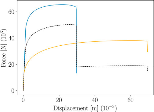
FIGURE 2. Main issue encountered when using standard interpolations on non-aligned curves (the black dashed line represents the interpolation between the two colored lines).

In what follows, we propose a procedure to overcome such spurious effects, based on a curve alignment prior to interpolate. The method is illustrated over the Force-Displacement curves. However, for the sake of generality, we refer to such curves as generic functions g(x), presenting two characteristic behaviors in the so-called primary and secondary zones. In the specific case of Force-Displacement, the primary zone is the elastic response of the material, up to the yield point x_E. The secondary zone is the post yield behaviour up to the failure point x_F, as illustrated in Figure 3. We will also refer to x_E as the “transition point” and to x_F as the “end point”, related to the specimen fracture.

FIGURE 3

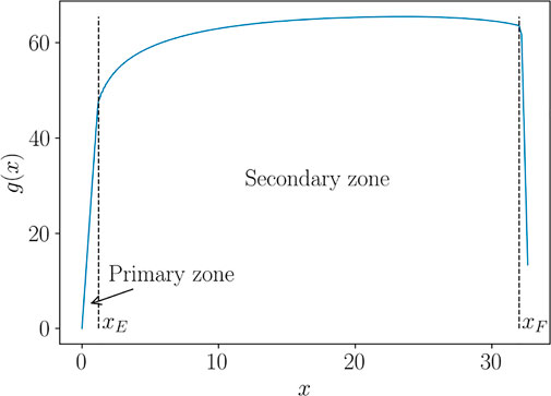
FIGURE 3. Behavior zones, transition and end points, for one function g(x).

We assume that the behaviors in the primary and secondary zone, g¹(x) and g²(x) respectively, and the transition and end points, x_E and x_F respectively, depend on a series of parameters grouped in vector p, i.e. g¹ (x; p) ≡ g (x ∈ [0, x_E]; p), g² (x; p) ≡ g (x ∈ [x_E, x_F]; p), x_E(p) and x_F(p). Indeed, when considering different choices of the model parameter p_i = (K_i, n_i, ɛ_0,i), i = 1, … , n_s, one obtains a set of curves, as the ones shown in Figure 4, for instance. Such curves correspond to a sparse DoE (Latin Hypercube) of 20 points in the 3-dimensional parametric space $\mathrm{\Omega }=I_K\times I_n\times I_{{\epsilon }_0}$, considering the parameters bounds specified in Table 1. Numerical simulations have been carried out with VPS simulation software from ESI Group. The variable x corresponds to the displacement in mm, while the function g(x) to the force in kN.

FIGURE 4

FIGURE 4. Curves g (x; p_i) related to different choices of the model features p_i = (K_i, n_i, ɛ_0,i), i = 1, … , n_s.

TABLE 1

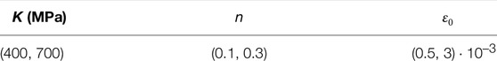
TABLE 1. Parametric ranges.

Once the transition and end points of each curve have been determined, the curves can be rediscretized over the same number of points (through a standard piecewise linear interpolation, for instance). To align them, we define a dimensionless coordinate in each zone, y in the primary zone, x ∈ [0, x_E], and z in the secondary zone, x ∈ [x_E, x_F], both defined through the change of variable

$y=\frac{x}{x_E},y\in \left[\mathrm{0,1}\right]\text{and}x\in \left[0,x_E\right],$

and

$z=\frac{x-x_E}{x_F-x_E},z\in \left[\mathrm{0,1}\right]\text{and}x\in \left[x_E,x_F\right],$

expressions that hold for each curve g (x; p_i), i = 1, … , n_s, with

$y=\frac{x}{x_E^i},y\in \left[\mathrm{0,1}\right]\text{and}x\in \left[0,x_E^i\right],$

and

$z=\frac{x-x_E^i}{x_F^i-x_E^i},z\in \left[\mathrm{0,1}\right]\text{and}x\in \left[x_E^i,x_F^i\right].$

Figure 5 depicts functions $g_i^1(y)\equiv g^1(y;{\mathbf{p}}_i)$ and $g_i^2(z)\equiv g^2(z;{\mathbf{p}}_i)$.

FIGURE 5

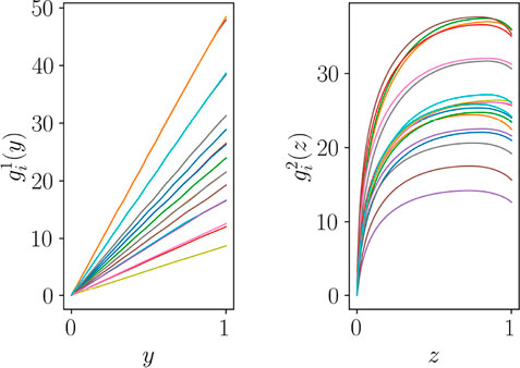
FIGURE 5. Functions $g_i^1(y)\equiv g^1(y;{\mathbf{p}}_i)$ (left) and $g_i^2(z)\equiv g^2(z;{\mathbf{p}}_i)$ (right), for i = 1, … , n_s.

Actually, this procedure amounts at performing an alignment based on a dilatation of the curves in the first and secondary zone, as shown in Figure 6. In such case, we can express the aligned curves as functions of $\tilde{x}\in [\mathrm{0,2}]$.

FIGURE 6

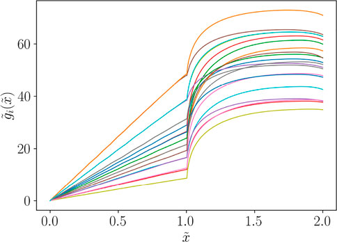
FIGURE 6. Functions ${\tilde{g}}_i(\tilde{x})$, for i = 1, … , n_s, obtained after dilatation.

Once the curves have been aligned, the nonlinear regressor presented in Subsection 2.3.3 can be invoked to build the parametric metamodel of the curve. This can be done separately in each zone or over the whole newly defined coordinate $\tilde{x}$. However, before proceeding with the regression, we address an ulterior parametrization via the Proper Orthogonal Decomposition to achieve a further Model Reduction as discussed in Paragraph 2.3.3.

3.1 POD Modes Extraction

In order to extract the most significant modes able to describe these functions, the POD can be applied in each group of curves in Figure 5. This amounts to build the snapshot matrix within each group and perform a truncated SVD. In the case that serves here to illustrate the procedure, a single mode suffices for describing the almost linear functions in the primary zone, that will be noted by ξ₁(y), whereas in the secondary zone two functions are needed, ϕ₁(z) and ϕ₂(z).

Thus, any function $g_i^1(y)$ can be expressed ∀i as

$g_i^1\left(y\right)={\alpha }_1^i{\xi }_1\left(y\right),$

whereas functions $g_i^2(z)$, ∀i, read

$g_i^2\left(z\right)={\beta }_1^i{\varphi }_1\left(z\right)+{\beta }_2^i{\varphi }_2\left(z\right).$

The α and β coefficients can be easily computed by simple projection, i.e.

${\int }_0^1{g}_i^1\left(y\right){\xi }_1\left(y\right)\mathrm{d}y={\alpha }_1^i,$

where the normality of ξ₁(y) was used. In the same way, and taking into account the orthonormality of functions ϕ₁(z) and ϕ₂(z),

${\int }_0^1{g}_i^2\left(z\right){\varphi }_1\left(z\right)\mathrm{d}z={\beta }_1^i,$

and

${\int }_0^1{g}_i^2\left(z\right){\varphi }_2\left(z\right)\mathrm{d}z={\beta }_2^i.$

Thus, for each curve g_i(x) we succeeded to extract its five main descriptors: $x_E^i,x_F^i,{\alpha }_1^i,{\beta }_1^i$ and ${\beta }_2^i$, all of them related to the features grouped in vector p_i.

Now, each of these descriptors can be expressed parametrically, x_E(p), x_F(p), α₁(p), β₁(p) and β₂(p), by using the regression techniques described in Subsection 2.3.1 for scalar quantities.

3.2 Curves Reconstruction

When considering a choice of the parameters p, the curves descriptors are extracted from the regressions x_E(p), x_F(p), α₁(p), β₁(p) and β₂(p), the dimensionless coordinates defining both zones calculated from

$y=\frac{x}{x_E\left(\mathbf{p}\right)}\to x=y{x}_E\left(\mathbf{p}\right),$

and

$z=\frac{x-x_E\left(\mathbf{p}\right)}{x_F\left(\mathbf{p}\right)-x_E\left(\mathbf{p}\right)}\to x=x_E\left(\mathbf{p}\right)+z\left(x_F\left(\mathbf{p}\right)-x_E\left(\mathbf{p}\right)\right),$

and, finally, the curve in each zone reconstructed according to

$g^1\left(y;\mathbf{p}\right)={\alpha }_1\left(\mathbf{p}\right){\xi }_1\left(y\right),$

and

$g^2\left(z;\mathbf{p}\right)={\beta }_1\left(\mathbf{p}\right){\varphi }_1\left(z\right)+{\beta }_2\left(\mathbf{p}\right){\varphi }_2\left(z\right),$

from which the curve g (x; p) can be straightforward obtained via

$g\left(x;\mathbf{p}\right)=\left\{\begin{array}{cc}{\alpha }_1\left(\mathbf{p}\right){\xi }_1\left(\frac{x}{x_E\left(\mathbf{p}\right)}\right),\hfill & x\in \left[0,x_E\left(\mathbf{p}\right)\right]\hfill \\ {\beta }_1\left(\mathbf{p}\right){\varphi }_1\left(\frac{x-x_E\left(\mathbf{p}\right)}{x_F\left(\mathbf{p}\right)-x_E\left(\mathbf{p}\right)}\right)+{\beta }_2\left(\mathbf{p}\right){\varphi }_2\left(\frac{x-x_E\left(\mathbf{p}\right)}{x_F\left(\mathbf{p}\right)-x_E\left(\mathbf{p}\right)}\right),\hfill & x\in \left[x_E\left(\mathbf{p}\right),x_F\left(\mathbf{p}\right)\right].\hfill \end{array}\right.$

To build the parametric metamodel, 17 curves have been used to train the sPGD regressor, while the remaining 3 for testing. Figure 7 shows the resulting predictions over 3 training points and test points.

FIGURE 7

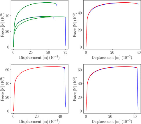
FIGURE 7. sPGD predictions (green line for training, red for testing) versus true curve (blue line).

3.3 Real-Time Calibration

Now, given an experimental curve g(x), its parameters are extracted according to.

• x_E from the point at which the change of behavior occurs (for instance, computing the function derivatives by means of finite differences);

• x_F is the terminal point;

• α₁ follows from $y=\frac{x}{x_E}$ and ${\int }_0^{1}g(y){\xi }_1(y)\mathrm{d}y={\alpha }_1$;

• β₁ follows from $z=\frac{x-x_E}{x_F-x_E}$ and ${\int }_0^{1}g(z){\varphi }_1(z)\mathrm{d}z={\beta }_1$;

• β₂ follows from $z=\frac{x-x_E}{x_F-x_E}$ and ${\int }_0^{1}g(z){\varphi }_2(z)\mathrm{d}z={\beta }_2$.

Then, from the regression models x_E(p), x_F(p), x₁(p), β₁(p) and β₂(p), the inverse problem is solved for extracting the associated parameters, p.

3.4 Statistical Model Derived by Parametric Curves

With the previously built surrogate model, the curve related to any possible value of p can be computed in real-time, i.e. g (x; p). In this section, this surrogate will be employed for uncertainty quantification.

We assume that each feature p^k in vector p is assumed characterized by a Gaussian distribution defined its mean value μ_k and its variance ${\sigma }_k^2$, that is $p^k\sim \mathcal{N}({\mu }_k,{\sigma }_k^2)$. Assuming all p^k being independent, we get

$\mathbf{p}\sim \mathcal{N}\left(\mathit{\mu },\mathbf{\Sigma }\right),\mathit{\mu }={\left({\mu }_k\right)}_{k=1}^d,\mathbf{\Sigma }=\text{diag}\left(\mathit{\sigma }\right),\mathit{\sigma }={\left({\sigma }_k^2\right)}_{k=1}^d,$

where diag (•) is the diagonal matrix of diagonal •.

The aim is linking the sensitivity over the input features with the one over the output curve. This means computing some estimators of the average M and the variance Σ of the curve descriptors for different choices of μ and σ, and from them, by using the regressions presented in Subsection 2.3, build the set of statistical surrogates:

$\left\{\begin{array}{c}{\mathcal{S}}_{g\left(x;\mathbf{p}\right)}:\left(\mathit{\mu },\mathit{\sigma }\right)\to \left({\bar{M}}_{g\left(x;\mathbf{p}\right)},{\bar{\mathrm{\Sigma }}}_{g\left(x;\mathbf{p}\right)}\right),\hfill \\ {\mathcal{S}}_{\mathcal{O}\left(\mathbf{p}\right)}:\left(\mathit{\mu },\mathit{\sigma }\right)\to \left({\bar{M}}_{\mathcal{O}\left(\mathbf{p}\right)},{\bar{\mathrm{\Sigma }}}_{\mathcal{O}\left(\mathbf{p}\right)}\right).\hfill \end{array}\right.(5)$

where $\mathcal{O}(\mathbf{p})$ denotes any QoI involved in the curves parametrization (i.e., an output depending on the input parameters; e.g., x_E, x_F, α₁, β₁ and β₂ in the example presented before) and $\bar{M}$ and $\bar{\mathrm{\Sigma }}$ the corresponding estimators for mean and variance, respectively. This allows calculating the envelopes, for a given confidence, of the curves, as sketched in Figure 8.

FIGURE 8

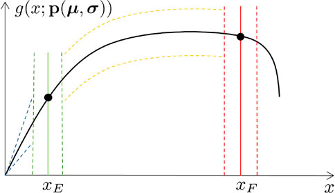
FIGURE 8. Sketch of curve envelopes.

To build the surrogate (5), for instance for the curve descriptor $\mathcal{O}(\mathbf{p})$, a training dataset of N_s points shall be generated:

${\left\{\left({\mathit{\mu }}_j,{\mathit{\sigma }}_j\right),\left({\bar{M}}_{\mathcal{O}\left({\mathbf{p}}_j\right)},{\bar{\mathrm{\Sigma }}}_{\mathcal{O}\left({\mathbf{p}}_j\right)}\right)\right\}}_{j=1}^{N_s}.$

This can be achieved by means of a Monte Carlo sampling, which gives the estimators of mean and variance for the curves g (x; p_j (μ_j, σ_j)), and of any descriptor $\mathcal{O}({\mathbf{p}}_j)$, for j = 1, … , N_s.

The whole procedure is summarized in Algorithm 1.

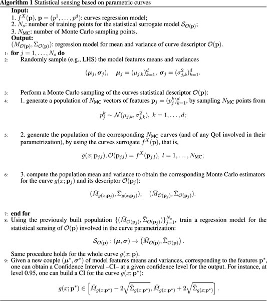
Figure 9 shows the parametric curve and its statistical sensing, for a given choice of the input features distribution parameters. Confidence Intervals have been computed using Algorithm 1, for the curve and the rupture point.

FIGURE 9

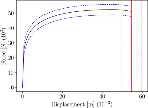
FIGURE 9. Confidence Interval of level 0.95 for the parametric Force-Displacement curve and for the rupture point, for a given choice of μ and σ.

3.5 Statistical Model Derived From Measures

In this Section we consider that for different choices of the problem features p_i, the measure g^m (x; p_i) is collected. We assume that measures contain a significant uncertainty, modeled again, without loss of generality, by a Gaussian distribution of null average and variance σ, that is, $\mathcal{N}(0,{\sigma }^2)$, with the variance assumed independent of the features p.

In these circumstances applying a regression to fit those values g^m (x; p_i), that is f^X,m (p_i) = g^m (x; p_i), according to the techniques described in Subsection 2.3 is not a valuable route. The most valuable solution consists of looking for the baseline regression f^X(p) such that the deviation ${\mathcal{D}}_i=f^{X,m}({\mathbf{p}}_i)-f^X(\mathbf{p})$ follows the distribution $\mathcal{N}(0,{\sigma }^2)$, where both the regression parameters involved in f^X(p) and the variance (if not known a priori) are calculated. In some cases the sensor calibration allows identifying σ².

The just described procedure is very close to standard Bayesian inference.

3.6 Model Enrichment

When two regression models are known, for the sake of simplicity assumed scalar, one related to a physics based model f^X,model(p) and the second one to the measures f^X,measure(p), both associated with the average values in case of uncertainty in the model and the measures, one could define the gap model Δf^X(p) from f^X,measure(p) − f^X,model(p) ≡Δf^X(p).

Thus, the enriched model reads

$f^{X,\text{enrich}}\left(\mathbf{p}\right)=f^{X,\text{model}}\left(\mathbf{p}\right)+\mathrm{\Delta }{f}^X\left(\mathbf{p}\right).$

As in general the nonlinear character of f^X,measure(p) is expected being much higher than the one of the gap, Δf^X(p), a more valuable route consists in calculating the discrete gap $\mathcal{D}({\mathbf{p}}_i)=f^{X,m}({\mathbf{p}}_i)-f^{\text{model}}({\mathbf{p}}_i)$ and then calculate the regression ${\widetilde{\mathrm{\Delta }f}}^X(\mathbf{p})$ fitting the discrete deviations, and the associated enriched model ${\tilde{f}}^{X,\text{enrich}}(\mathbf{p})$

${\tilde{f}}^{X,\text{enrich}}\left(\mathbf{p}\right)=f^{X,\text{model}}\left(\mathbf{p}\right)+{\widetilde{\mathrm{\Delta }f}}^X\left(\mathbf{p}\right).$

4 Data Alignment and Data Clustering

Here we focus on the study of crack propagation in notched specimens loaded in tension, whose geometry is sketched in Figure 10. The test piece has a V-shaped notch defect which is always at the same location (almost bottom-middle). On the other side of the test piece there is a half-circle groove. The goal is to predict the crack propagation from the defect based off of different locations (S) and radii (R) of the groove, as well as different test piece thicknesses (h). Depending on the location of the groove, the crack will propagate differently from the defect to the groove.

FIGURE 10

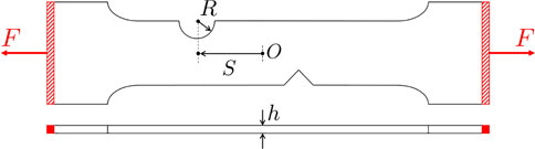
FIGURE 10. Parametric notched dog bone specimen loaded in tension (top and side views).

We have considered a sparse DoE (Latin Hypercube) of 50 points in the 3-dimensional parametric space Ω = I_R × I_S × I_h, with the parameters bounds specified in Table 2. Numerical simulations (carried out in VPS software from ESI Group) employ an Explicit Analysis and the EWK rupture model (Kamoulakos, 2005), using a mesh of 1096218 solid elements.

TABLE 2

TABLE 2. Parametric ranges.

We focus on the prediction of the Force-Displacement curves plotted in Figure 11, which are considered as the generic functions g(x), following the same notation of Section 3.

FIGURE 11

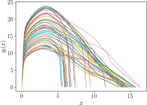
FIGURE 11. Curves g_i(x) = g (x; p_i) related to different choices of the model features p_i = (R_i, S_i, h_i), i = 1, … , n_s.

It can be observed that all the curves present a similar pattern in the first zone, monotonically increasing, while the response appears much different in the secondary zone. A first pre-processing step consists in splitting the zones as illustrated in Figure 12, where x_M denotes the point where the curve reaches its maximum value, while x_F its endpoint.

FIGURE 12

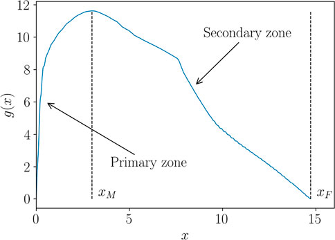
FIGURE 12. Behavior zones, transition and end points, for one function g(x).

Cutting the curves, we obtain the two groups of functions plotted in Figure 13, which are of course not aligned. However, they can be expressed as functions of normalized coordinates y and z, respectively, and aligned following the dilatation procedure discussed in Section 3.

FIGURE 13

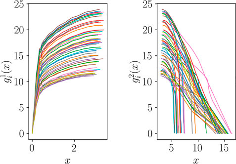
FIGURE 13. Functions $g_i^1(x)\equiv g^1(x;{\mathbf{p}}_i)$ (left) and $g_i^1(x)\equiv g^2(x;{\mathbf{p}}_i)$ (right), with p_i = (R_i, S_i, h_i), for i = 1, … , n_s.

Once the alignment has been performed, using the usual nonlinear regression techniques of Subsection 2.3 and same notations of Section 3, two regression models, one for each group, can be established:

$\left\{\begin{array}{c}{g}^1\left(x;\mathbf{p}\right):=g\left(x\in \left[0,x_M\left(\mathbf{p}\right)\right]\right)=f_1^X\left(\mathbf{p}\right)\hfill \\ g^2\left(x;\mathbf{p}\right):=g\left(x\in \left[x_M\left(\mathbf{p}\right),x_F\left(\mathbf{p}\right)\right]\right)=f_2^X\left(\mathbf{p}\right).\hfill \end{array}\right.(6)$

In Eq. 6, for the sake of clarity, we have specified x_M and x_F since these points are involved into the parametrization of the functions g¹(x) and g²(x), respectively, and thus expressed parametrically.

As we have previously pointed out, the second group of functions $g_i^2(x)$, for i = 1, … , n_s, presents really different shapes depending on the features p_i. When bifurcations occur in the parametric space, the system responses related to two choices of the model parameters can be completely different. In such cases, a standard nonlinear regression over the full space can lead to inaccurate and nonphysical solutions. To enhance the accuracy of the model $f_2^X(\mathbf{p})$, a more valuable route consists in exploring the parametric space prior to interpolation. This can be done via a clustering of the system responses. Once the clusters have been established, several regression sub-models can be built, minimizing the risk of mixing spurious effects coming from other clusters.

4.1 Clustering

To exemplify the bifurcation problem in the parametric space, we consider two different configurations of the model parameters, resulting into the specimens shown in Figure 14.

FIGURE 14

FIGURE 14. Two different parameters configurations. Top: R = 7.59, S = 18.23, h = 0.84; bottom: R = 3.75, S = 5.58, h = 1.51 (all dimensions are provided in mm). The red zone is the part subject to rigid body constraints.

Figure 15 shows four snapshots of the displacement field related to the specimens in Figure 14, under axial tensile loading. The crack propagation follows two completely different patterns, drastically influencing the Force-Displacement curve, as shown in Figure 16.

FIGURE 15

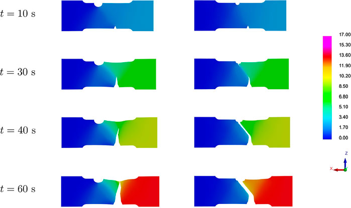
FIGURE 15. Bifurcation in the parametric space causing completely different crack propagation dynamics.

FIGURE 16

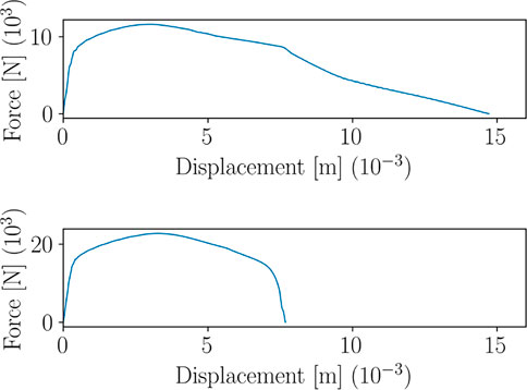
FIGURE 16. Force-Displacement curves corresponding to the two parameters configurations in Figure 14.

The clustering step can be performed automatically by using a hierarchical clustering based on the curves shape or on the location of damaged elements into the finite element mesh. Once the clusters ${\mathcal{C}}_1$ and ${\mathcal{C}}_2$ have been established, two regression submodels can be trained, one for each cluster, and Eq. 6 becomes

$\left\{\begin{array}{c}{g}^1\left(x;\mathbf{p}\right)=f_1^X\left(\mathbf{p}\right)\hfill \\ g^2\left(x;\mathbf{p}\right)=\left\{\begin{array}{cc}{f}_{\mathrm{2,1}}^X\left(\mathbf{p}\right)\hfill & \text{for\hspace{0.17em}}{\mathcal{C}}_1\hfill \\ f_{\mathrm{2,2}}^X\left(\mathbf{p}\right)\hfill & \text{for\hspace{0.17em}}{\mathcal{C}}_2.\hfill \end{array}\right.\hfill \end{array}\right.(7)$

Figure 17 shows the functions in the secondary zone after the clustering.

In particular, one can remark that fracture occurs early on for tests belonging to cluster ${\mathcal{C}}_1$ and the final part of the curve is characterized by a steep slope. On the contrary, tests belonging to cluster ${\mathcal{C}}_2$ have an endpoint displacement around 15 mm and present a shallow slope. The clustering allows to avoid averaging such different dynamics, clearly enhancing the quality of the regressor.

FIGURE 17

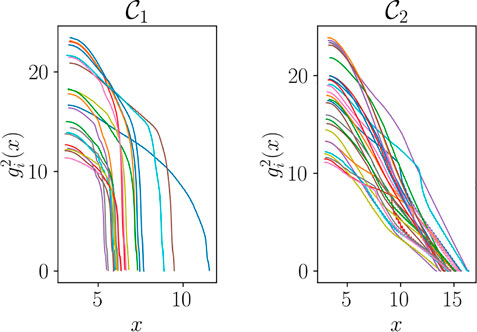
FIGURE 17. Functions $g_i^2(x)$ of Figure 13 (right) after clustering, for i = 1, … , n_s.

4.2 Curves Reconstruction and Classification

For a newly defined choice of model features p^*, the curve g (x; p^*) is obtained via

$g\left(x;{\mathbf{p}}^{*}\right)=\left\{\begin{array}{cc}{g}^1\left(x;{\mathbf{p}}^{*}\right),\hfill & 0\le x\le x_M\left({\mathbf{p}}^{*}\right)\hfill \\ g^2\left(x;{\mathbf{p}}^{*}\right),\hfill & x_M\left({\mathbf{p}}^{*}\right)<x\le x_F\left({\mathbf{p}}^{*}\right),\hfill \end{array}\right.$

where g¹ and g² are obtained through Eq. 7.

The training of the regression models has been performed using 40 points of the DoE, remaining 10 have been used for testing. Moreover, a Support Vector Machine classifier (a Random Forest classifier could also be used, for instance) has been trained to select the best regression submodel to predict g² (x; p^*). Such classifier has shown perfect accuracy, as shown by the Confusion Matrices in Figure 18. Moreover, Figure 19 shows the separating surface and classified points in the 3-dimensional parametric space.

FIGURE 18

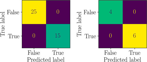
FIGURE 18. Confusion Matrices for the SVM classifier (left: training data, right: test data).

FIGURE 19

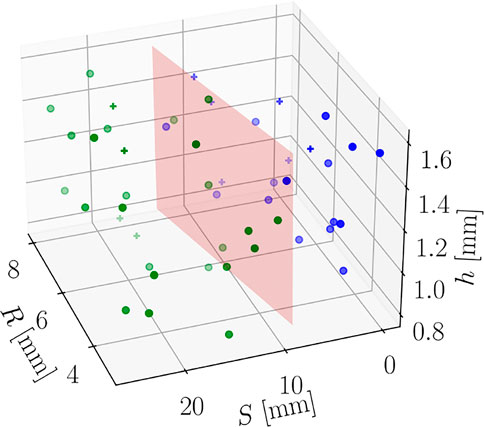
FIGURE 19. Parametric space and classified points (marker + is used for test points). The red plane is the separation surface.

Figures 20, 21 represent the plots of predictions for train and test, respectively, for 4 data points.

FIGURE 20

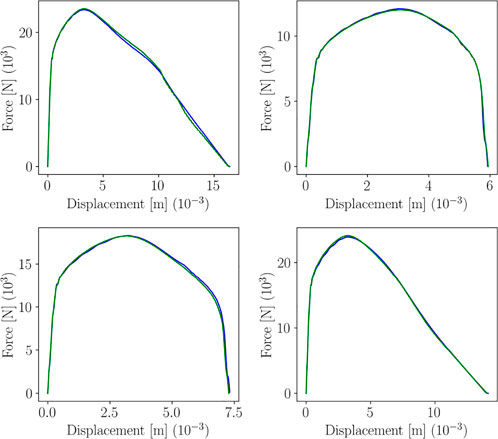
FIGURE 20. sPGD predictions (green line) versus true curve (blue line) for training data.

FIGURE 21

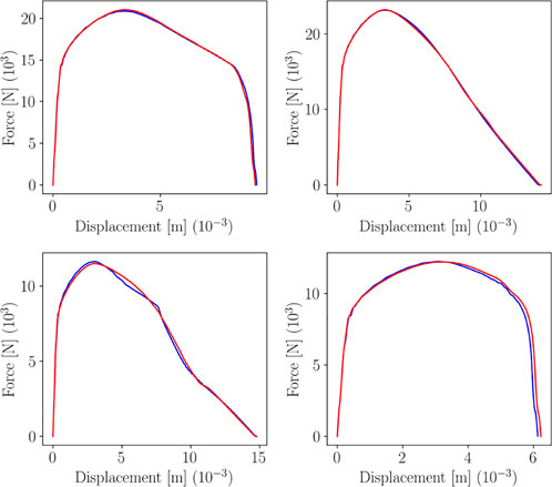
FIGURE 21. sPGD predictions (red line) versus true curve (blue line) for test data.

5 Conclusion

In this paper we have focused on several nontrivial issues encountered when a whole curve shall be predicted from a given number of features. A major argument is the data alignment to achieve physics-consistent interpolations among curves and the data clustering to detect bifurcations in the parametric space. The proposed methodologies rely on adopting specific parametrizations of the curve and a physics-based pre-processing prior to the application of any regression technique. We have also suggested a reduced order parametrization of the curve via POD coefficients, requiring the prediction of a few scalar quantities (i.e., the POD coefficients) instead of the whole curve. Here, without loss of generality, we have preferred sPGD-based nonlinear regressions, these being efficient in high-dimensional parametric spaces under the scarce data limit constraint. Indeed, since our data come from numerical simulations of complex engineering problems, due to the high computational complexity of the offline simulations, not much data are usually available. Moreover, one important achievement of the work is the definition of a statistical sensing for uncertainty propagation based on the parametric model.

We have focused on two applications in computational mechanics: 1) plastic materials with parametric hardening law, 2) crack propagation in parametric notched specimens. However, these methodologies can be applied to any time series or generic curve stem from any context. For instance, in our current research, we are successfully applying these techniques to solve many other problems (to cite some, the study of a two-phase flow dynamics in a heated channel, the composite forming processes involving a reactive resin injection molding). Moreover, we are focusing on other physics-based curves interpolation strategies based on Optimal Transport–OT–(Torregrosa et al., 2022) and other mappings.

Data Availability Statement

The raw data supporting the conclusions of this article will be made available by the authors, without undue reservation.

Author Contributions

All the authors participated in the definition of techniques and algorithms. All authors read and approved the final manuscript.

Conflict of Interest

The authors declare that the research was conducted in the absence of any commercial or financial relationships that could be construed as a potential conflict of interest.

Publisher’s Note

All claims expressed in this article are solely those of the authors and do not necessarily represent those of their affiliated organizations, or those of the publisher, the editors and the reviewers. Any product that may be evaluated in this article, or claim that may be made by its manufacturer, is not guaranteed or endorsed by the publisher.

Acknowledgments

The authors acknowledge the support of ESI Group through its research chair at ENSAM ParisTech. This research is part of the programme DesCartes and is supported by the National Research Foundation, Prime Minister’s Office, Singapore under its Campus for Research Excellence and Technological Enterprise (CREATE) programme.

References

Amsallem, D., and Farhat, C. (2008). Interpolation Method for Adapting Reduced-Order Models and Application to Aeroelasticity. AIAA J. 46, 1803–1813. doi:10.2514/1.35374

CrossRef Full Text | Google Scholar

Audouze, C., De Vuyst, F., and Nair, P. B. (2013). Nonintrusive Reduced-Order Modeling of Parametrized Time-dependent Partial Differential Equations. Numer. Methods Partial Differ. Eq. 29, 1587–1628. doi:10.1002/num.21768

CrossRef Full Text | Google Scholar

Benner, P., Schilders, W., Grivet-Talocia, S., Quarteroni, A., Rozza, G., and Silveira, L. M. (2020a). Model Order Reduction: Applications. Berlin: De Gruyter.

Google Scholar

Benner, P., Schilders, W., Grivet-Talocia, S., Quarteroni, A., Rozza, G., and Silveira, L. M. (2020b). Model Order Reduction: Snapshot-Based Methods and Algorithms. Berlin: De Gruyter.

Google Scholar

Benner, P., Schilders, W., Grivet-Talocia, S., Quarteroni, A., Rozza, G., and Silveira, L. M. (2020c). Model Order Reduction: System- and Data-Driven Methods and Algorithms. Berlin: De Gruyter.

Google Scholar

Benner, P., Gugercin, S., and Willcox, K. (2015). A Survey of Projection-Based Model Reduction Methods for Parametric Dynamical Systems. SIAM Rev. 57, 483–531. doi:10.1137/130932715

CrossRef Full Text | Google Scholar

Borzacchiello, D., Aguado, J. V., and Chinesta, F. (2017). Non-intrusive Sparse Subspace Learning for Parametrized Problems. Arch. Comput. Methods Eng. 26, 303–326. doi:10.1007/s11831-017-9241-4

CrossRef Full Text | Google Scholar

Chinesta, F., Ladeveze, P., and Cueto, E. (2011). A Short Review on Model Order Reduction Based on Proper Generalized Decomposition. Arch. Comput. Methods Eng. 18, 395–404. doi:10.1007/s11831-011-9064-7

CrossRef Full Text | Google Scholar

Cristianini, N., and Shawe-Taylor, J. (2000). An Introduction to Support Vector Machines and Other Kernel-Based Learning Methods. Cambridge: Cambridge University Press.

Google Scholar

de Gooijer, B. M., Havinga, J., Geijselaers, H. J. M., and Van den Boogaard, A. H. (2021). Evaluation of Pod Based Surrogate Models of Fields Resulting from Nonlinear Fem Simulations. Adv. Model. Simul. Eng. Sci. 8. doi:10.1186/s40323-021-00210-8

CrossRef Full Text | Google Scholar

Fareed, H., and Singler, J. R. (2019). A Note on Incremental Pod Algorithms for Continuous Time Data. Appl. Numer. Math. 144, 223–233. doi:10.1016/j.apnum.2019.04.020

CrossRef Full Text | Google Scholar

Franchini, A., Sebastian, W., and D'Ayala, D. (2022). Surrogate-based Fragility Analysis and Probabilistic Optimisation of Cable-Stayed Bridges Subject to Seismic Loads. Eng. Struct. 256, 113949. doi:10.1016/j.engstruct.2022.113949

CrossRef Full Text | Google Scholar

Friderikos, O., Baranger, E., Olive, M., and Néron, D. (2022). On the Stability of Pod Basis Interpolation on Grassmann Manifolds for Parametric Model Order Reduction. Comput Mech. Cham: Springer. doi:10.1007/s00466-022-02163-0

CrossRef Full Text | Google Scholar

Friderikos, O., Olive, M., Baranger, E., Sagris, D., and David, C. N. (2020). A Space-Time Pod Basis Interpolation on Grassmann Manifolds for Parametric Simulations of Rigid-Viscoplastic Fem. MATEC Web Conf. 318, 01043. doi:10.1051/matecconf/202031801043

CrossRef Full Text | Google Scholar

Hesthaven, J. S., Rozza, G., and Stamm, B. (2016). Certified Reduced Basis Methods for Parametrized Partial Differential Equations. Cham: Springer. doi:10.1007/978-3-319-22470-1

CrossRef Full Text | Google Scholar

Hesthaven, J. S., and Ubbiali, S. (2018). Non-intrusive Reduced Order Modeling of Nonlinear Problems Using Neural Networks. J. Comput. Phys. 363, 55–78. doi:10.1016/j.jcp.2018.02.037

CrossRef Full Text | Google Scholar

Hilberg, D., Lazik, W., and Fiedler, H. E. (1994). The Application of Classical Pod and Snapshot Pod in a Turbulent Shear Layer with Periodic Structures. Appl. Sci. Res. 53, 283–290. doi:10.1007/bf00849105

CrossRef Full Text | Google Scholar

Ibáñez, R., Abisset-Chavanne, E., Ammar, A., González, D., Cueto, E., Huerta, A., et al. (2018). A Multidimensional Data-Driven Sparse Identification Technique: The Sparse Proper Generalized Decomposition. Complexity 2018, 1–11. doi:10.1155/2018/5608286

CrossRef Full Text | Google Scholar

Kamoulakos, A. (2005). “The ESI-Wilkins-Kamoulakos (EWK) Rupture Model,” in Continuum Scale Simulation of Engineering Materials: Fundamentals - Microstructures - Process Applications (Hoboken: John Wiley & Sons), 795–804. doi:10.1002/3527603786.ch43

CrossRef Full Text | Google Scholar

Khatouri, H., Benamara, T., Breitkopf, P., and Demange, J. (2022). Metamodeling Techniques for Cpu-Intensive Simulation-Based Design Optimization: a Survey. Adv. Model. Simul. Eng. Sci. 9. doi:10.1186/s40323-022-00214-y

CrossRef Full Text | Google Scholar

MacQueen, J. B. (1967). “Some Methods for Classification and Analysis of Multivariate Observations,” in Proc. Of the Fifth Berkeley Symposium on Mathematical Statistics and Probability. Editors L. M. L. Cam., and J. Neyman (California: University of California Press), 281–297.

Google Scholar

Mainini, L., and Willcox, K. (2015). Surrogate Modeling Approach to Support Real-Time Structural Assessment and Decision Making. AIAA J. 53, 1612–1626. doi:10.2514/1.J053464

CrossRef Full Text | Google Scholar

Mosquera, R., El Hamidi, A., Hamdouni, A., and Falaize, A. (2021). Generalization of the Neville-Aitken Interpolation Algorithm on Grassmann Manifolds: Applications to Reduced Order Model. Int. J. Numer. Meth Fluids 93, 2421–2442. doi:10.1002/fld.4981

CrossRef Full Text | Google Scholar

Mosquera, R., Hamdouni, A., Hamdouni, A., El Hamidi, A., and Allery, C. (2018). Pod Basis Interpolation via Inverse Distance Weighting on Grassmann Manifolds. Discrete Continuous Dyn. Syst. - S 12, 1743–1759. doi:10.3934/dcdss.2019115

CrossRef Full Text | Google Scholar

Prud’homme, C., Rovas, D. V., Veroy, K., Machiels, L., Maday, Y., Patera, A. T., et al. (2002). Reliable Real-Time Solution of Parametrized Partial Differential Equations: Reduced-Basis Output Bound Methods. J. Fluids Eng. 124, 70–80. doi:10.1115/1.1448332

CrossRef Full Text | Google Scholar

Raghavan, B., Hamdaoui, M., Xiao, M., Breitkopf, P., and Villon, P. (2013). A Bi-level Meta-Modeling Approach for Structural Optimization Using Modified Pod Bases and Diffuse Approximation. Comput. Struct. 127, 19–28. doi:10.1016/j.compstruc.2012.06.008

CrossRef Full Text | Google Scholar

Rajaram, D., Perron, C., Puranik, T. G., and Mavris, D. N. (2020). Randomized Algorithms for Non-intrusive Parametric Reduced Order Modeling. AIAA J. 58, 5389–5407. doi:10.2514/1.J059616

CrossRef Full Text | Google Scholar

Sancarlos, A., Champaney, V., Duval, J., Cueto, E., and Chinesta, F. (2021). Pgd-based Advanced Nonlinear Multiparametric Regressions for Constructing Metamodels at the Scarce-Data Limit. CoRR abs/2103.05358, ArXiv.

Google Scholar

Simpson, T. W., Poplinski, J. D., Koch, P. N., and Allen, J. K. (2001). Metamodels for Computer-Based Engineering Design: Survey and Recommendations. Eng. Comput. 17, 129–150. doi:10.1007/PL00007198

CrossRef Full Text | Google Scholar

Torregrosa, S., Champaney, V., Ammar, A., Herbert, V., and Chinesta, F. (2022). Surrogate Parametric Metamodel Based on Optimal Transport. Math. Comput. Simul. 194, 36–63. doi:10.1016/j.matcom.2021.11.010

CrossRef Full Text | Google Scholar

Wang, G. G., and Shan, S. (2007). Review of Metamodeling Techniques in Support of Engineering Design Optimization. J. Mech. Des. 129, 370–380. doi:10.1115/1.2429697

CrossRef Full Text | Google Scholar