Efficient reconstruction of prior austenite grains in steel from etched light optical micrographs using deep learning and annotations from correlative microscopy

The high-temperature austenite phase is the initial state of practically all technologically relevant hot forming and heat treatment operations in steel processing. The phenomena occurring in austenite, such as recrystallization or grain growth, can have a decisive influence on the subsequent properties of the material. After the hot forming or heat treatment process, however, the austenite transforms into other microstructural constituents and information on the prior austenite morphology are no longer directly accessible. There are established methods available for reconstructing former austenite grain boundaries via metallographic etching or electron backscatter diffraction (EBSD) which both exhibit shortcomings. While etching is often difficult to reproduce and strongly depend on the investigated steel’s alloying concept, EBSD acquisition and reconstruction is rather time-consuming. But in fact, though, light optical micrographs of steels contrasted with conventional Nital etchant also contain information about the former austenite grains. However, relevant features are not directly apparent or accessible with conventional segmentation approaches. This work presents a deep learning (DL) segmentation of prior austenite grains (PAG) from Nital etched light optical micrographs. The basis for successful segmentation is a correlative characterization from EBSD, light and scanning electron microscopy to specify the ground truth required for supervised learning. The DL model shows good and robust segmentation results. While the intersection over union of 70% does not fully reflect the model performance due to the inherent uncertainty in PAG estimation, a mean error of 6.1% in mean grain size derived from the segmentation clearly shows the high quality of the result.

Introduction

Steel is still the world’s most important engineering and construction material due to its excellent combination and customizability of properties through tailored microstructures. A special trait of steel respectively iron is its polymorphism, i.e., it shows different crystal structures depending on the temperature. The body-centered cubic ferrite phase is present at room temperature, while the face-centered-cubic austenite phase is present at elevated temperatures. In steel manufacturing, hot-forming and heat treatment operations often take place in the austenite phase. After these operations, the steel is cooled down to room temperature, and in case of low-alloyed steels, transforms to varying room temperature microstructures like ferrite-pearlite, bainite, or martensite, depending on cooling rate and chemical composition. The evolution of the austenite grain size during hot forming or heat treatment as well as the final resulting austenite grain size are of high importance as they either affect the processes or significantly influence the type and properties of the final microstructure.

The introduction of thermo-mechanically controlled processing (TMCP) has been one of the most significant developments in steel processing, regarding product quality as well as economic efficiency (Zhao and Jiang, 2018). Investigating how the austenite grain size evolves during the entire TMCP, from grain growth during slab reheating to recrystallization during rough hot rolling stages to pancaking in the final hot rolling stages, is crucial for understanding the TMCP as well as for modelling it. This in turn is the basis for continued process optimization and steel development.

The final austenite grain size after hot forming or heat treatment, before cooling the steel, greatly influences the phase transformation behavior and thereby the resulting microstructure. In general, large austenite grain sizes correspond to fewer nucleation sites for phase transformations when cooling down from the austenite which promotes diffusion-less martensitic transformation over diffusion-dependent transformations, e.g., pearlite or bainite (Bargel and Schulze, 2005). Regarding the martensitic transformation, finer austenite grains can reduce the size of martensitic substructure and increase the density of high misorientation angle boundaries after quenching (Hidalgo and Santofimia, 2016) as well as lower the martensite start temperature and increase the initial transformation rate (Celada-Casero et al., 2019). It is well known that the toughness of steels can be improved by grain refinement (Gottstein, 2014). Related to bainitic and martensitic steels, refining prior austenite grains (PAG) is considered the first step in their microstructural refinement (Li et al., 2022). Controlling the austenite grain size is also used for improving other properties, e.g., refining the austenite grain size for enhancing the abrasive wear resistance of ultra-high strength martensitic steels (Haiko et al., 2020), improving the temper embrittlement resistance of Cr-Mo steels (Khan and Islam, 2007; Karthikeyan et al., 2017) or increasing amount and stability of retained austenite in an austempered low-carbon bainitic steel to achieve high-strength/high-toughness combinations (Lan et al., 2017), amongst others. During multi-pass welding of linepipe steels, the size of martensite–austenite constituents in the heat affected zone (HAZ) can be reduced and the HAZ toughness improved by controlling the maximum austenite grain size (Li et al., 2014).

Hence, it is of paramount importance to measure and quantify the prior austenite grain size. However, for the investigated low-alloy steels, austenite is only present during forming or heat treatment at higher temperatures, but not in the final microstructure which poses the greatest challenge in the assessment of the austenite grain size. Various approaches to measure the prior austenite grain size, with their own, procedure-inherent advantages and disadvantages, exist. Moreover, all approaches have a particular degree of uncertainty in common since PAG are not directly accessible.

PAG size can be measured indirectly by laser ultrasonic through the scattering by discontinuities like grain boundaries (Militzer et al., 2012). However, due to the indirect nature of the measurement, there are many parameters than can influence the result and an elaborate verification of the procedure is necessary.

In contrast to the indirect measurements, PAG reconstruction using orientation data from electron backscatter diffraction (EBSD) yields not only mean grain sizes but grain size distributions and is spatially resolved. This reconstruction method can be applied if the product of the phase transformation during cooling nucleates and grows inside its parent grain with a known orientation relation (OR) (Germain et al., 2012). For steel, this applies to the OR between austenite (parent phase) and martensite respectively bainite (product or child phases). PAG reconstruction by EBSD has become widespread in the last years and is readily available in various commercial or open-source software packages. Approaches for reconstructing PAG include (Cayron, 2007; Germain et al., 2012; Nyyssönen et al., 2016; Niessen et al., 2022). Disadvantages are the time-consuming EBSD measurement and computationally expensive reconstruction. Additionally, preliminary work showed that the reconstruction works well mostly for martensitic steels but performs worse on bainitic constituents.

The most widely used methods for determining PAG size are probably still metallographic techniques for which several approaches exist. One is to highlight PAG by preferred oxidation or precipitation, according to the methods of Kohn or McQuaid-Ehn described in international standards (ISO 643:2019 Steels—Micrographic determination of the apparent grain size, no date). When applying them, however, it must be kept in mind that microstructural features will be changed by the heat treatment needed for oxidation/precipitation and that they are not suitable for any steel type. Thermal etching (García De Andrés et al., 2001; García de Andrés et al., 2002; Pöhl et al., 2009; San Martín et al., 2010) can also be used to delineate PAGs, however, the expensive equipment as well as traces of old grooves from the grain growth process are drawbacks (García de Andrés et al., 2002). Usually, chemical etching is preferred due to its simple application without the need for special experimental devices. The etching after Bechet-Beaujard, a saturated aqueous picric acid solution with the wetting agent sodium alkylsulfonate (Bechet and Beaujard, 1955) is well-established and widespread for quenched or quenched and tempered steels. It is assumed that the effect of the etchant is based on attacking micro segregations of phosphorus (Ucisik et al., 1978). Hence, steels with low phosphorus contents, i.e., below 0.05% cannot be reliably contrasted (Ogura et al., 1978). Additionally, this etching is not always working for low and ultra-low carbon steels. Tempering the sample at 650°C has been reported to improve the contrasting but is not always recommendable due to altering the microstructural features. In general, chemical etchings for delineating PAG can be hard to reproduce, vary depending on the chemical composition of the investigated steel and be especially challenging for low phosphorous and/or carbon levels. Furthermore, to achieve sufficient contrasting, multiple steps of etching combined with back-polishing can be necessary.

Most of the time, the PAG contrasting might be visible and distinguishable for the observer, and sufficient for determining mean grain sizes by comparison with reference states. However, when an automated quantification and determination of grain size distributions through computer vision is strived for, the etchants often exhibit insufficient selectivity to reliably distinguish substructures inside the PAG from PAG boundaries (PAGB). For steels, the so-called Nital etching, a mixture of ethanol and nitric acid, is one of the standard etchants for analyzing the microstructures of un- and low-alloyed steels. Due to its simplicity and ease of use, it is very popular. Although Nital is originally not intended for PAG contrasting, it reveals several information about them. PAGB can either rendered visible directly due to topography differences or can be recognized indirectly based on orientations of martensitic and bainitic laths or sub-units. But since all other hierarchical microstructure features are also contrasted, a PAG segmentation using conventional methods is not possible.

Here deep learning (DL) comes into play. One common DL technique is based on convolutional neural networks (CNN) which has led to a paradigm shift in image processing. The main advantage of such representation learning methods is that they not only learn the classification process itself, but simultaneously identify the features needed for this classification (Forsyth, 2019). Thereby, DL can solve tasks for which simple deterministic, rule-based solutions do not work. Research fields like autonomous driving and biomedicine acted as driving forces for the application and spread of DL (Ronneberger et al., 2015; Saleh et al., 2018; Natekar et al., 2020) but by now it is well established in the materials science community, too. Especially for microstructure analysis, i.e., the segmentation and classification of micrographs, it offers promising new potentials. Besides providing improved reproducibility, objectivity, and automation, it can enable tasks where conventional methods reached their limits.

Azimi et al. (2018) applied DL to classify the carbon-rich second phase in dual-phase steels into pearlite, bainite, martensite and tempered martensite. DeCost et al. (2019) segment varying constituents in high-carbon steels. Durmaz et al. (2021) used DL to segment lath-shaped bainite in complex-phase steel microstructures, based on annotations from correlative EBSD data. Numerous examples for DL segmentation of grain or cell structures, across different domains, can also be found, e.g., (Konovalenko et al., 2018a; Konovalenko et al., 2018b; Bordignon et al., 2019; Furat et al., 2019; Pazdernik et al., 2020; Das et al., 2022). In a recent publication, the authors also applied DL to improve the automated PAG quantification based on new chemical etching on the basis of Bechet-Beaujard for improved delineation of PAG (Laubet al., Forthcoming 2022). Due to the importance of this topic on the one hand, and its diversity with many possible research directions on the other hand, it is currently dealt with in a large consortium, consisting of all contributing institutions. The consortium follows the objective of finding an optimal methodology and learning strategy to reliably detect PAGB in a wide variety of martensitic and bainitic steels.

This paper represents the first publication of the consortiums’ joint work. It focuses on the detection of PAG in Nital-etched light optical micrographs of bainitic and martensitic steels, implemented by a semantic segmentation (pixel-wise classification) using established, state-of-the-art DL methods. Particular attention is paid to the quality of the training data for the DL segmentation. Therefore, correlative characterization combining light optical microscope, scanning electron microscope, as well as electron backscatter diffraction is used to accomplish a well-funded, objective, and reproducible ground truth needed for training a DL model. The model is not only evaluated by standard ML metrics, but also by determining the accuracy of mean grain sizes and grain size distributions of the DL segmentation. Furthermore, the robustness of the DL model regarding etching artefacts and image acquisition settings will be analyzed.

Materials and methods

Material

As investigated material, quenching dilatometry samples (5 mm diameter) of a low carbon steel [0.088% C with a CEV of 0.53% (I.I.W.)] with different cooling rates, each austenitized at 950°C, were used. The cooling rates during the quenching range from 2.5°C/s up to 3,600°C/s. The microstructural phases can be identified as martensite and bainite. A selection of used optical micrographs after Nital etching, representing the material’s microstructure, are shown in Figure 1.

FIGURE 1

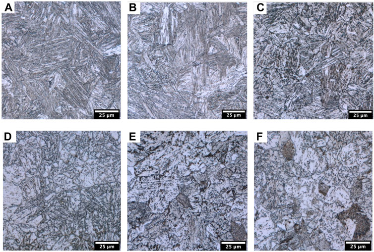
FIGURE 1. A selection of optical micrographs of representative sections of the used samples. The cooling rates of the quenching are: (A) 3,600°C/s, (B) 2,400°C/s, (C) 300°C/s, (D) 56°C/s, (E) 15°C/s, (F) 5°C/s. The samples shown in (A) and (B) show purely martensitic microstructures and (C—F) show mainly bainitic microstructures. Sample (C) show lath-like bainitic microstructures that show visual similarities to martensitic packages. The bainitic samples (D—F) illustrate the continuously increasing amount of carbon depletion in more distinctive carbon rich phases.

Correlative microscopy

Samples are characterized by applying a correlative microscopy approach in which samples are analyzed by light optical microscope (LOM), scanning electron microscope (SEM) as well as electron backscatter diffraction (EBSD). In general, correlative microscopy approaches allow to combine advantages of several methods, eliminate disadvantages, and merge information from complementary sources and across different length scales. In addition, it is possible to gain insights and references via the additional methods in the correlative approach and to reduce later evaluations to one, the simplest, method (Durmaz et al., 2021; Müller et al., 2021). In this work, the additional correlative measurements with SEM and EBSD are used for establishing the ground truth/annotations for the PAG segmentation in the LOM images.

Correlative characterization was done according to the method we previously published (Müller et al., 2021). All samples were ground using 80–1,200 grid SiC papers, and then subjected to 6, 3, and finally, 1 μm diamond polishing. For investigation by EBSD, colloidal oxide polishing was additionally performed after diamond polishing. To be able to find and characterize the exact same area of a sample with different methods, a region of interest (ROI) must be marked. For this purpose, a ROI is marked using hardness indentations in the form of an equilateral triangle of HV0.5 indents, with a base and height of 500 µm each.

First, the EBSD measurement is performed, as it is usually done on a non-etched sample surface. A Zeiss Merlin FEG-SEM was used with an acceleration voltage of 25 kV, a probe current of 10 nA, and 15 mm working distance. Areas of 400 × 400 µm were scanned with a step size of 0.35 μm using a hexagonal grid, at a magnification of ×200. The software EDAX OIM Data Collection (Version 7, 2015) was used. After EBSD measurements, samples were re-polished for about 1 minute to remove the contamination on the sample surface introduced by the EBSD measurement, subsequently etched with 2.5 vol% Nital solution (2.5 ml nitric acid, 97.5 ml ethanol) for about 15 s and micrographs from the same ROI were taken in LOM and SEM. For LOM images, the light optical microscope of an Olympus LEXT OLS 4100 laser scanning microscope was used. Images were taken at a magnification of ×1,000 with an image size of 1,024 × 1,024 pixels, corresponding to an area of 129.6 × 129.6 μm (pixel size = 126.6 nm). All images were acquired with the same image contrast and brightness settings. For SEM images, a Zeiss Merlin FEG-SEM using secondary electron contrast at a magnification of ×850 with an image size of 2048 × 1,536 pixels, corresponding to 97.2 × 72.9 μm (pixel size = 47.5 nm) was used. The SEM was operated at an acceleration voltage of 5 kV, a probe current of 300 pA, and a working distance of 5 mm. All images were acquired with the same image contrast and brightness settings in the SEM. To capture the entire ROI, multiple images must be acquired for both LOM and SEM. Images were taken with a certain overlap and then stitched together.

To be able to combine the information from different imaging techniques, the different resulting images must be registered. The term image registration is defined as the “overlay of (two or more) images of an identical area, obtained at different points in time, from different angles and/or with different sensors” (Zitová and Flusser, 2003). Simple superpositions of these microstructural images purely by rotational or translational adjustments are usually not possible, since the physics underlying the image generation can be very different for the different methods. For a general explanation of challenges during correlative characterization and image registration in metallography, the authors refer to Britz et. Al Britz et al. (2017a). In previous works, image registration was successfully applied using the plugins SIFT feature extraction and bUnwarpJ in the open-source software ImageJ to the correlative characterization with LOM, SEM and EBSD of industrial two-phase and multi-phase steels (Britz et al., 2017a; Britz et al., 2017b; Müller, Britz and Mücklich, 2021). The Scale-Invariant-Feature Transform (SIFT (Feature Extraction - ImageJ, no date)) algorithm is used first to locate the same features in an EBSD map and the LOM and SEM image. The image quality map is a suitable representation of the EBSD data as it has a similar appearance to the other modalities. The common features from SIFT feature extraction are then used to perform the image registration using the bUnwarpJ (BUnwarpJ - ImageJ, no date) algorithm. The transformation matrix that is calculated during registration can later be used to register other EBSD-derived maps, e.g., misorientation maps. For more details about the correlative approach the authors refer to (Müller et al., 2021).

Compared to the previously studied two-phase and multi-phase steels, the quenched and tempered steels with fully bainitic or martensitic microstructures show a higher complexity with more homogeneous structures as well as lower overall contrast differences, which makes it challenging to automatically find common features for image registration. In fact, automatic SIFT feature extraction was only possible for coarse bainitic structures, for fine bainitic or martensitic structures it was neither possible with SIFT nor with other state-of-the-art feature extraction techniques. Hence, for the image registration, a manual selection of point correspondences is necessary. During this elaborate task, common features, such as triple points of the PAG, are marked in LOM and respective EBSD IQ map. The number of selected correspondences has a large influence on the quality of the registration. After collecting a representative number of correlating landmarks, in this showcase at least 25 corresponding features per image were manually selected, the image registration has been executed using the bUnwarpJ algorithm. The effort of correlative characterization has to be done only once, for generating the training data set for DL. An everyday series application will be done with only LOM images.

EBSD reconstruction of prior austenite grains

The crystallographic reconstruction of the PAG, needed for the ground truth for the training data set, has been done using the MATLAB R2021b toolbox MTEX 5.7 (Bachmann et al., 2010; Niessen et al., 2022) provide a workflow, which loads the raw EBSD data and reconstructs the PAG using different preprocessing steps and filters. For the final reconstruction, similarly oriented child grains within the PAG with a tolerance of 12.5° have been filtered, using the function mergeSimilar. Besides, default settings according to (Bachmann et al., 2010; Niessen et al., 2022) were applied. One big advantage of the MTEX workflow, compared to others like (Cayron, 2007), is the ability to iteratively adjust the respective OR of the parent grain starting from one of the well-known OR (Nishiyama-Wassermann, Kurdjumow-Sachs or Greninger-Troiano), yielding better reconstruction results. For further information, the authors refer to the respective literature.

Annotations and final data set

The quality of the final dataset is essential to assure a well-engineered and reliable segmentation pipeline. Although creating the masks is based on the EBSD PAG reconstruction, manual corrections of the masks are inevitable. Due to the working principle of the crystallographic reconstruction, it is mostly limited to martensitic microstructures. The higher the phase fraction of the bainitic microstructural constituents, the less reliable the reconstruction results become. Here, manual corrections of the PAGB come into play. To obtain objective and valid ground truth assignments, LOM and the high-resolution SEM images are overlayed with the PAG reconstruction, in order to correct the boundaries within the masks. The high-resolution SEM allows to more objectively identify visual features of PAGB based on the pronounced topography contrast in the SEM. The boundaries in the final masks, consisting of the manual corrected EBSD reconstruction, have a width of nine px. As postprocessing, the course of the annotated boundaries was smoothened using a median filter with a setting of eight px. Creating the dataset including masks is a very time consuming and elaborate step in the presented procedure. Though, it is crucial for the learning process of the used segmentation pipeline. If the masks do not fit the visual PAGB in the optical micrographs, learning can be prolonged if there are contradictions, since the model tries to learn visual features, which do not correspond to the correct labels. Preliminary tests showed that using the EBSD reconstruction without manual corrections would strongly degrade the segmentation model performance.

The final dataset consisted of 13 different dilatometry samples, each with a different cooling rate, including correlative data (13 LOM, 13 SEM and eight EBSD) and manually adjusted masks. Each image covers sample regions of size 400 × 400 µm² containing approximately 250 PAGs in average. The corresponding resolution of the. tif format images is 4096 × 4096 px (pixel size of 97.7 nm).

Deep learning methodology

Through different layer architectures, CNNs obtain their ability to process image data reproducibly in order to fulfil specific tasks. The loss function is a measure for the model’s adaption to the respective task and is minimized during the training process. The parameters within the network’s architecture, such as the settings of the filter kernels to extract the proper feature maps, are adjusted in order to optimize the density of the extracted information. Ronneberger et al. Ronneberger et al. (2015) presented a groundbreaking segmentation pipeline based on CNNs, originally developed for medical image analysis, the so-called “UNet”. It consists of two segments, one encoding part, compressing the image information into a latent space representation, and one decoding part, expanding the information in order to reconstruct a segmented image of the original input. Through the encoder-decoder mechanism, not only the semantic information of the image’s content can be extracted, but also the spatial information (Ronneberger et al., 2015) which allows to create meaningful segmentation maps as outputs. In addition to contraction and extraction path, there are connections between the different levels of encoder and decoder (skip-connections) resulting in a beneficial behavior of the model’s convergence. Also, through skipping the convolutions and pooling operations, finer details can be retained for the final segmentation, since the information is not influenced by the gradient descent during the training in the encoding procedure. Another beneficial aspect of the UNet is the ability to work well with even very few training images in combination with data augmentation. Therefore, it is very attractive to domains, where it is difficult to gather large-scale data sets, as it is usually necessary for DL applications.

The DL pipeline is based on the segmentation models package (Iakubovskii, 2022) which uses the Keras environment, implemented in python 3.8. Training was executed in Google Colab Pro, using a Nvidia Tesla P100 GPU. In the segmentation models package, the respective backbone of the encoder can be chosen out of a selection of the common CNN architectures. The input of the UNet are the sliced patches of the micrographs. Based on the fact that this showcase represents a binary classification problem, the output of the UNet is binary, representing the PAGB segmentation of those patches. Based on the corresponding masks that are one-hot-end-encoded to be handled by the DL approach, the model’s parameters are optimized during training in order to yield an image segmentation result that shows the least possible error to the respective masks.

During training the frozen encoder weights from the available architectures, respectively pretrained on the ImageNet database, consisting of more than 14 million natural images, were applied. This concept, the so-called transfer learning (Tammina, 2019), relies on the assumption that the weights of the architecture’s layers, thus the filter kernels, are already well adjusted to detect low-level, as well as high-level visual features. Another significant difference between UNet and the traditional CNN for classification is the size-independence of the input (Azimi et al., 2018). Whereas CNNs for classification tasks can only handle images with the same input as the training images, UNet does not make use of fixed-size dense layers, which are necessary for classification, and thus the limiting factor of the input size. Therefore, the UNet architecture can be trained on small patches and subsequently do inference on entire microstructural images.

Before the actual training process, different preprocessing steps must be applied to the original images. First, they need to be split into individual patches. Here, the patch size must be selected adequately to ensure that individual patches contain sufficient long-range features to detect PAGB. Since grain boundaries are not as frequent, the images are downscaled before tiling to increase the feature density per patch. Thus, more context per patch can increase the segmentation performance in cases where the focus lays on long-scale features, such as grain boundaries (Goetz et al., 2022). To provide more context information of the different patches (256 px patch size), the images have been cropped with a respective overlap of 56 px. Using those settings, overall, 1,420 final patches have been created for training, validation and testing (data splits of 75%, 15%, 10%, respectively).

The validation data set is used during the training to validate the training process and prevent overfitting. The test dataset is used for independent testing and subsequent comparison of the differently trained models. The best model has been selected based on the used metrics, as well as on the performance on the unseen testing-dataset, also regarding the suitability for subsequent postprocessing, which has been evaluated by a materials science expert. For training, an extensive data augmentation pipeline has been implemented, as it is necessary to yield reliable results, especially due to the data scarcity of microscopic images: rotation (65°), shift (15%), shear (10%), zoom (20%) as well as vertical and horizontal flip have been used. The missing edges, as result of the augmentation process, have been filled by reflections of the border regions. Finally, the well-established preprocessing-step of rescaling the pixel values (between 0 and 255) to a range between 0 and one and normalizing each color channel based on the mean pixel value of the ImageNet database, as recommended when using these pre-trained weights.

For semantic segmentation it has been established to use intersection over union (IoU) as metric, being a measure of overlap between predictions and ground truth, since it is more sensitive and representative for segmentation tasks with unbalanced data like here, than traditional metrics such as pixel accuracy (Rahman and Wang, 2016). As described above, the loss function can be seen as a numerical representation of the DL algorithm’s objective. Thus, a considered selection is essential for a well-adjusted segmentation pipeline (Rahman and Wang, 2016). In this case, the two classes for segmentation (PAGB and interjacent hierarchical microstructure) are highly imbalanced. Hence, a weighted dice loss function, considering the total amount of pixels of each class has been proven to be beneficial. Furthermore, an equally weighted, binary-crossentropy Jaccard loss has been implemented, by adding it to the dice loss function yielding the final loss term. It refers to a linear combination of a traditional binary-crossentropy loss and a Jaccard loss (Wang et al., 2020), with the latter being a representation the used metric of IoU. Earlier experiments (Laubet al., Forthcoming 2022) have shown that this combination of loss functions and architecture works reliably for boundary segmentation tasks. As backbone the DenseNet (Huang et al., 2017) has been selected. Compared to well-known architectures, such as VGG, Inception or ResNet it shows superior results in preliminary tests. This can be concluded from earlier work. Reason for this could be the high interconnectivity between the different layers within DenseNet’s architecture (Huang et al., 2017). This leads to an improved information flow throughout the network, which makes them not only to reuse crucial information, but also to be more efficient. As learning rate for the Adam optimizer a value of 0.001 was selected and the batch size was set to 8.

Post-processing of deep learning segmentation

Following the segmentation, a post-processing of the segmentation result map is performed. Due to the use of the softmax function, the segmented image is not a binary mask, but a greyscale probability map. First greylevel threshold (50%) is performed, followed by an area-opening (removing objects <500 px) to remove small objects that were mistakenly segmented as grain boundaries. Second, a watershed algorithm is used to complete grain boundaries that were only partially segmented. As algorithm, the distance transform watershed from Fiji’s Plugin MorphoLibJ (Legland et al., 2016) was used. For the initial distance transform, Borgefors’ setting (Feng and Wettlaufer, 2018) was used and the dynamic parameter of the subsequent flooding was chosen to be between 5 and 10, depending on the segmentation result.

Since pixel accuracy and IoU do not fully express the model performance, as will be discussed in the next section, and ultimately, it is not about values of these metrics, but about how exactly the grain sizes are measured, the output segmentation map, after post-processing, is quantified to determine the grain size distribution. From the distribution, several mean values (area fraction mean, number fraction mean, median) as well as the standard deviation are calculated and compared to values and distribution of the ground truth to get additional criteria to evaluate the segmentation quality and assess the potential errors in grain size determination. In order to determine the area fraction grain size, all detected grains have been binned (bin width = 500 µm²) and the probability density has been calculated.

Results and discussion

Before discussing segmentation results, the ground truth assignment must be discussed. The ground truth for the LOM images is based on correlative SEM images and EBSD measurements which was the most objective and reproducible way possible. In fact, without this correlative data, the annotations could not have been created at all. However, there is still a remaining uncertainty and subjectivity. The austenite phase is the high temperature phase that is not present anymore in the final microstructure at room temperature, and there is no method available that can determine the PAG beyond all doubt. As illustrated in Figure 2, the EBSD reconstruction method itself does not delineate the PAG fully and correctly. Additionally, the result strongly depends on the parameters and filters used during the EBSD-based reconstruction. Hence, manual corrections based on SEM images are needed which in turn can be partially subjective, e.g., when PAG are not fully contrasted from the etching and their path must be partially anticipated by the human expert. Thus, there is an uncertainty inherent to the task of determining PAG which will be fully present in any training data and ground truth and is expected to reflect in performance metrics of the DL model.

FIGURE 2

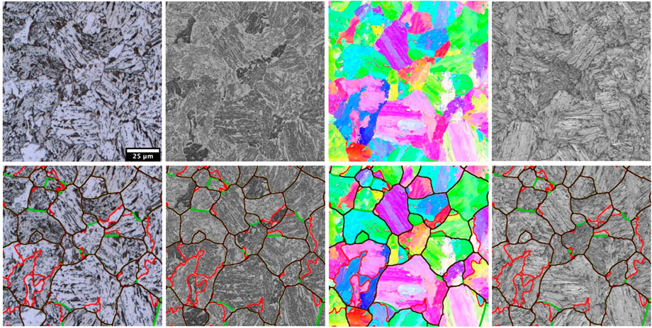
FIGURE 2. Overview of the different correlative data (left to right: LOM, SEM, IPF, IQ) with discrepancies (lower) between EBSD reconstruction (red) and manual annotation (green) and the overlapping sections between EBSD reconstruction and manual annotations (black).

The final model was trained for 15 epochs and achieved an overall IoU of 0.73 ± 0.005 on the training dataset and 0.70 ± 0.007 on the validation dataset and a F1 score of 0.82 ± 0.004 and 0.80 ± 0.006, respectively. The training process on a Nvidia Tesla GPU took about 1 h. It is noticeable that the model converges very quickly and achieves a relatively high IoU (>65%) already after three epochs. Reasons for this could be the usage of the UNet in combination with DenseNet as encoder backbone as well as the training data quality. The DenseNet architecture is well known for a high efficiency which can be traced back to the parameter reuse and the ability to systematically gather “collective knowledge” through the high interconnectivity (Huang et al., 2017). Towards the end of the training process, the model starts to slightly overfit, which can be seen in the beginning divergence of the performances on training and validation dataset (Figure 3). Hence, the training process is stopped at that point, where both training and validation IoU reach 70%.

FIGURE 3

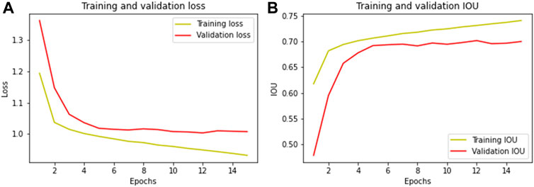
FIGURE 3. Metrics [(A): Loss, (B): IOU] of the model during training and validation.

For this segmentation task, the overall IoU of about 70% gives a very conservative estimation of the model performance. This can be attributed to the uncertainty of PAG determination as well as the annotation process. Also, not only IoU is considered, but patches of the unseen validation dataset are evaluated and show very promising segmentation results (Figure 4). Though, it should be mentioned that through the data preparation routine, a certain overlap between training and validation patches can occur and thereby influence the metric IoU. For this segmentation task, the IoU, although it is state-of-the-art metric in the field of semantic segmentation, cannot exclusively be used for quantifying the quality of the model. The measurement of the IoU is based on the overlap of the segmented pixels compared to the pixels, assigned to the corresponding classes, in the ground truth mask. In this case, a problem arises due to the process of annotations. The pixel width of the boundaries in the ground truth mask has to be chosen considerably. As the masks are provided by correlative EBSD reconstructions and SEM images, the quality of the registration between EBSD map, SEM image and LOM image plays a significant role.

FIGURE 4

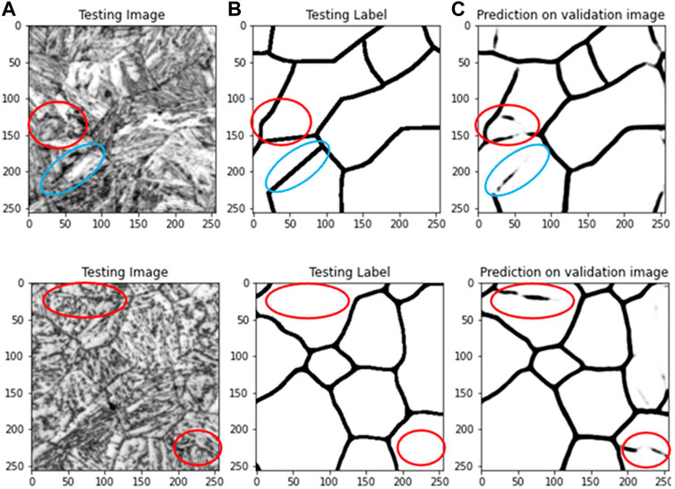
FIGURE 4. Representative patches of LOM micrographs (upper: martensitic, lower: bainitic) from unseen validation dataset (A), the corresponding ground truth label (B) and the prediction of the final model before post-processing (C). Due to the softmax function, applied to the output, the segmentation result is a greyscale image, representing the predicted probability of the respective class.

There are cases where there is a slight misalignment between masks and visual PAGB features within the LOM. There, the masks must be dilated until the regions of the actual PAGBs are covered, i.e., the masks can cover bigger areas than just the PAGB. There, a lower IoU for the segmentation result can be expected. For this, a compromise must be found between actual pixel width of the PAGBs in the Nital-etched micrograph and the quality of the annotated masks. Due to this fact, a domain-specific quantitative analysis of the segmentation result is desired. A comparison of the grain size distributions of the post-processed and the annotated ground truth will be conducted in the further course of this work, to reliably quantify the quality of the segmentation results.

In case of the martensitic samples, most part of the PAGBs can be segmented correctly, though, some parts are not closed or show slightly different courses (Figure 4, blue). Since the working principle of CNNs is based on apparent visual features, it cannot reliably detect features of existing PAGBs, that are not visible. Here, the importance of a well etched micrograph should be mentioned. The model most likely would not be able to reconstruct PAGBs, if none of them is contrasted. This explanation can be supported through the slightly better segmentation in bainitic samples, where the contrast between boundaries and actual “grains” is higher than it is the case in martensitic microstructures. Slower cooling rates allow that more alloying elements can diffuse towards the boundaries, as it is the case in bainitic microstructures. Though, in bainitic microstructures not only the PAGB are contrasted, but additionally the visible packet boundaries. The occasional gaps in the segmented PAGB network can be closed for further quantitative grain size analysis, using the described watershed segmentation algorithm.

Reason for the fact that some regions of the PAGBs are not segmented correctly can be found in the visual appearance of martensitic and bainitic microstructures. Through their lath-like shape, some packet boundaries potentially could be interpreted as PAGBs, as it is the case in the red marked regions in Figure 4. Without much context to the surrounding grains, it is reasonable that the model mistakenly segments packet borders as PAGBs, since it is even human experts cannot undeniably distinguish one from another. To resolve the problem of the misleading segmentation artefacts, the area opening post-processing step will be included to the entire segmentation pipeline.

Figure 5 displays the different post-processing steps. As mentioned before, the segmentation results were binarized using a grey-level threshold, followed by the area opening step to remove segmentation artefacts. Subsequently the watershed algorithm allows filling the different gaps in the PAGB network in order to yield closed grains to be able to fulfill quantitative grain analysis.

FIGURE 5

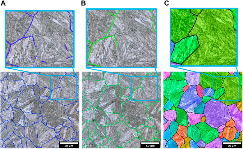
FIGURE 5. (A): LOM of sample B (cooling rate of 2,400°C/s) with overlayed segmentation result (blue) (B): LOM with segmentation result after area opening step (green). (C): LOM micrograph with reconstructed PAGB (black) and colored PAG labels after watershed segmentation.

The entire PAGB reconstruction process including segmentation and post-processing took less than 1 min per input image (4096 × 4096 px2, corresponding to an area of 400 × 400 µm²). At first glance, the reconstruction shows a good agreement with the annotation. Although, the watershed segmentation leads to unnaturally straight boundaries in regions, where larger gaps must be filled. After the area opening step, some of the misleading artefacts that are connected to the rest of the segmented PAGBs are still present and not connected to any other boundaries, though, based on the dynamics settings in the watershed algorithm, they do not negatively influence the final filling step, as can be seen in Figure 5 (right), and thus, the grain size measurement. Depending on the segmentation result based on the respective input image, the settings of the post-processing procedure, such as the area opening pixel threshold value, and the dynamic parameter of the watershed flooding can be adjusted in order to optimize the reconstruction result. In a potential implementation, a semi-automated pipeline demanding the post-processing parameters, such as area opening threshold and the dynamic parameter of the watershed algorithm, this problem can be addressed in order to achieve a better adjustability to the respective segmentation result.

For the quantitative analysis, three, mainly martensitic samples A, B and C with the cooling rates 3,600°C/s, 2,400°C/s and 1800°C/s, respectively, have been chosen. Excerpts of final segmentation results of the selected samples, including the segmented PAGBs after the area opening step and the grain color labels based on the watershed segmentation, are shown in Figure 6.

FIGURE 6

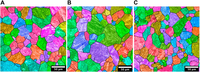
FIGURE 6. Segmentation result after area opening (black) including watershed segmentation color labels for validation samples (A), (B), and (C).

It is noticeable that there are PAGs, that are not correctly reconstructed. Reasons for that, such as insufficient contrasting, as well as packet boundaries that are wrongly segmented as PAGB, have been described above. In the following paragraph, the actual influence of those deviations on the measured grain size distribution and mean grain sizes is presented.

Overall, the grain size parameters of the reconstruction nicely match those of the ground truth for the most part (Figure 7). It is noticeable that the area fraction mean grain size parameters of the reconstruction, as well as the standard deviation, consistently underestimate the actual grain sizes to a small degree. Despite most of the artefacts of the segmentation can be cleaned through the area opening step, some of the remaining ones lead to undesired fillings during watershed, systematically leading to smaller overall grains. Figure 5 and the area fractions of the smaller-sized grains (Figure 7) in the grain size distribution support this assumption. Although this problem could not be tackled completely in scope of this work, an optimized post-processing pipeline, eventually even with manual corrections, in cases where high accuracies are desired, can help to improve the reconstruction result. Additionally, due to the systematic nature of this error, it can be possible to calculate the real grain size from the segmented grain size by accounting for the average deviation. Furthermore, it needs to be mentioned that the analyzed region is relatively small, which leads to a higher influence of statistical errors. Increasing the size of the region that should be measured might lead to better results due to the lower impact of the segmentation errors. Nevertheless, the presented results are promising and show the high potential of the presented workflow. This approach has many advantages to any other state-of-the-art approach for determining the PAG grain size, additionally delivering a segmentation of the PAGB network for further analysis, such as grain extraction or morphological analysis. It should also be mentioned that the current practice to quantify PAG after metallographic etching is mostly still a comparison with grain size standard diagrams from international standards. Thus, in cases where the DL segmentation results are not sufficient for watershed post-processing and determination of a reasonable grain size distribution, the segmentation results will always be good enough to at least determine an average grain size using standard diagrams. Here, the importance of the use of the domain knowledge should be pointed out. Despite it could be put more emphasis on the optimization process of the model, the focus was held on a holistic approach and the embedding of the DL approach within a efficient and reproducible workflow. Thereby the domain-based weaknesses, especially the contrasting method could be tackled successfully. Since it is feasible in the field of metallography to always assume perfectly contrasted micrographs, a robust post-processing routine, combining the traditionally use of morphological image processing steps and the implementation of the well-tried watershed segmentation. Furthermore, the entire pipeline is more flexible to higher variances in the segmentation results due to inhomogeneities in the contrasted micrographs. It is well-known, that a better generalizability comes along with a loss of total accuracy, but this postprocessing routine is able to tackle this negative side effect and makes the detection process of the PAGB more robust.

FIGURE 7

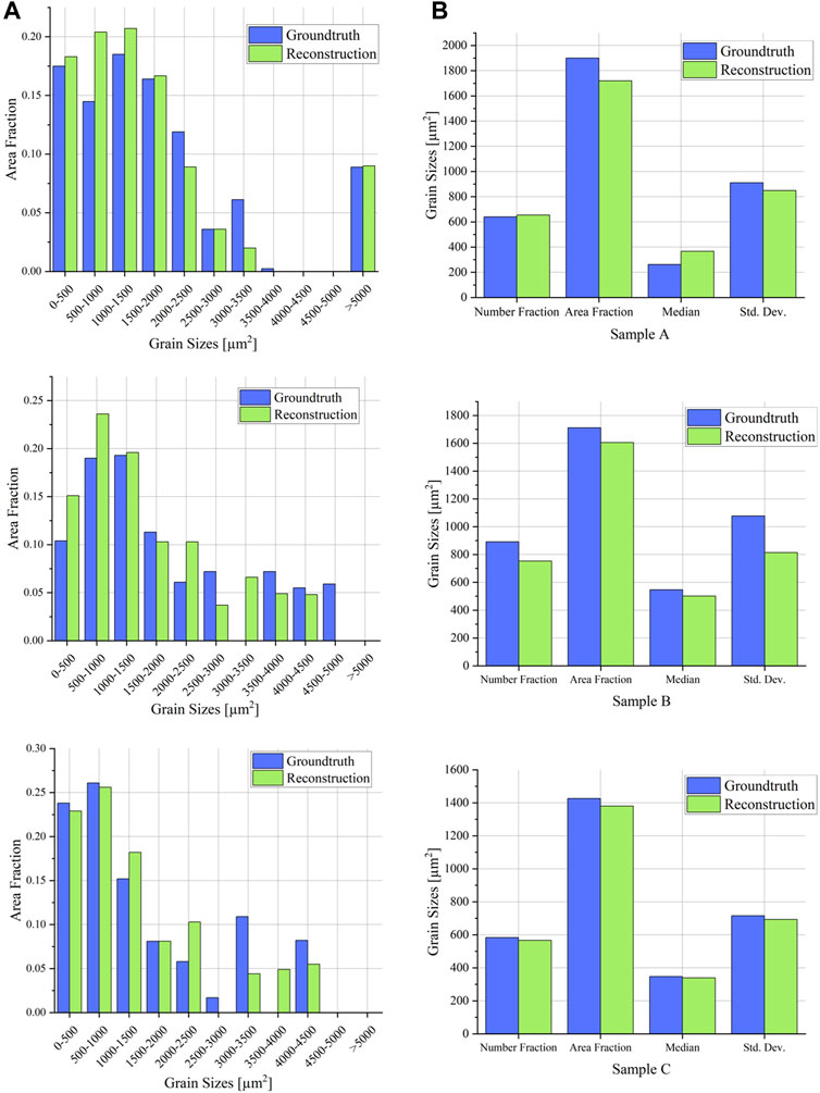
FIGURE 7. Comparison of the segmentation results to corresponding ground truths of the three validation samples. (A): grain size distribution, (B): characteristic grain size parameters. The deviation between the grain sizes between reconstruction and groundtruth is only small. Sample C containing a higher amount of bainitic microconstituents shows the least difference. The area fraction mean grain size of the martensitic sample A contains the highest error, underestimating the grain sizes. With decreasing cooling rates that error becomes less noticeable.

In the following paragraph the focus is held on the segmentation result of bainitic samples. Due to the transformation character, the boundaries of the bainite packets cannot always be equated to the boundaries of the prior austenite grains. Figure 8 visualizes the hierarchical character and differences of boundaries in bainitic microstructures.

FIGURE 8

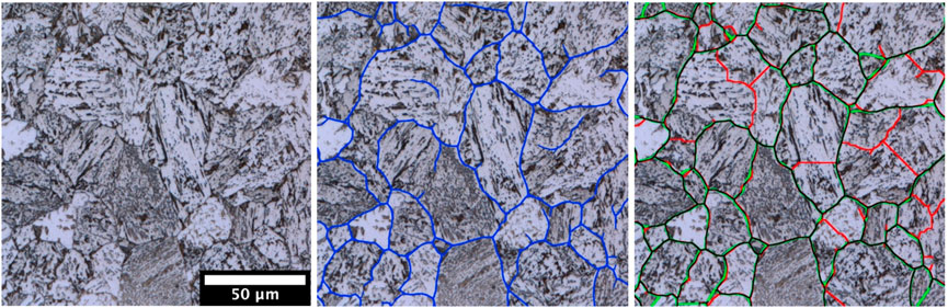
FIGURE 8. Excerpt of an LOM of a bainitic sample with a cooling rate of 15°C/s (left), showing the segmented boundaries after area opening (blue) and the watershed segmentation result (right) with the overlap (black) between groundtruth (green) and post-postprocessed segmentation result (red).

This is a known problem in PAG reconstruction using metallographic etching as well as EBSD. This means that for bainitic microstructures our DL model will segment both PAG and bainite packet boundaries. The currently available data of Nital-etched LOM and SEM as well as correlative ESBD reconstruction does not yet enable a further distinction of PAG and bainite packet. Still, a segmentation of bainite packets is an important quantification as they contain undeniably important information about the material’s microstructure and allow correlations to mechanical properties as well. Furthermore, it is conceivable to infer the PAG size from the segmented packet size. Figure 8 illustrates the performance of the final model, metrics shown in Figure 3, detecting the boundaries of PAG and bainite packets. Most of the parts of the segmented boundaries match those of the ground truth. The same post-processing as described for the martensitic samples can be applied.

In Figure 9 the direct comparison of the grain reconstruction of a martensitic and a bainitic sample is shown. In both cases an evaluable result could be achieved to get further information about the morphology of the microstructural constituents.

FIGURE 9

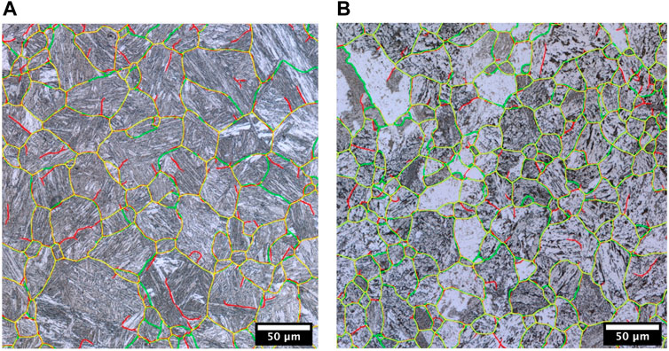
FIGURE 9. Excerpts of a LOM micrograph with post-processed segmentation result (red), ground truth annotation (green) and overlap between both (yellow) for a martensitic (A) and a bainitic sample (B).

Due to the variances that can arise in metallography during everyday work, e.g., variances in sample preparation, sample contrasting or image acquisition, it is important to evaluate the robustness of the DL model. To determine the variance that the model can handle, non-optimal micrographs are being analyzed. On one side, a micrograph showing slight etching artefacts is being segmented and post-processed and on the other side, inference on an artificially blurred image, simulating image acquisition without proper focusing, is executed.

Even though etching artefacts cover the areas of important visual features, all boundaries can be segmented (Figure 10). The quality of the result is remarkable, considered the condition of the input image. Apparently, the model is robust enough to reliably fulfill the trained task, as long as significant visual features are present. A human expert probably would have considerable problems to annotate micrographs, showing such intensities of etching artefacts. In cases where all visual features are removed due to bad contrasting, watershed post-processing potentially could still yield a decent result. For possible series application, the robustness of the model could even be improved by specifically using training datasets that also include lower grade micrographs, showing worse contrasts and artefacts, in order to cover the variance in a practical application.

FIGURE 10

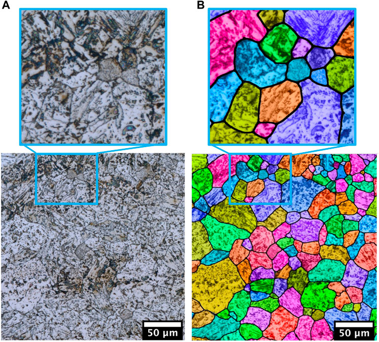
FIGURE 10. LOM micrograph of an unseen sample with etching artefacts (A) and the segmentation result after postprocessing (B) showing the color-labeled grains from the reconstruction.

Figure 11 shows that the model is able to detect the majority of the boundaries, even in blurred images. This also supports the conclusion of a robust model. Though, some regions, especially where an already low contrasted region gets degraded by the blur filter, the model is not able to segment most of the boundary parts. Since semantic segmentation is based on the presence of visual features, it is always desired to only use input images, captured under good conditions, comparable to conditions of generating the training data set. Loss of important features leads to a loss in quality of the segmentation result. There is a possibility to use unsharp training images as well, although this might be accompanied with a model that has a higher generalizability, but a lower overall quality. Hence, it is always desired to only use high-quality input images, if possible. More experiments could be executed in order to investigate the quality of the segmentation results based on further common artefacts originated in the sample preparation, such as scratches. Since scratches show similar visual features to some PAGB, it could be interesting to characterize the influence of this possible problem.

FIGURE 11

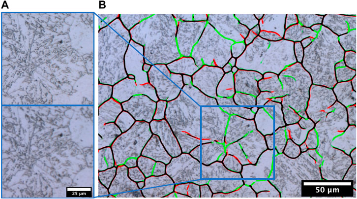
FIGURE 11. Testing model on blurred micrograph (A) (mean filter—three px: left upper shows sharp micrograph-left lower shows blurred micrograph). Overlay of the segmentation results, without any post-processing [(B)—green: original image, red: blurred image, black: overlap between the segmentations].

The amount of the used data in the training dataset sounds undersized, compared to common DL datasets. Though, natural images, such as in ImageNet, cannot directly be compared to microscopic images. Durmaz et al. Durmaz et al. (2021) could achieve very good results using before mentioned CV approaches using very little data. Reason for this being the high feature density and comparatively lower variance of microscopic images of microstructures: Moreover, the number of objects of interests is usually orders of magnitudes higher for microstructural images, than for natural images (here: several grains respectively boundaries per image, compared to e.g., one cat). There is almost no meaningless background, which has to be identified as such, and ignored. Also, images are always acquired with the same perspective in the microscope, in contrast to natural images. Furthermore, the spatial relationship and length scales, e.g., magnifications, are physically based and rather discrete than continuous (Thomas et al., 2020).

The basis for the successful implementation of this processing pipeline is the quality of the used data. Thanks to correlative microscopy, information from LOM, SEM and crystallographic EBSD information could be combined. Using only one of those information sources to tackle this problem of segmentation would lead to considerably worse results. Using only EBSD reconstructions without manual corrections would distort the training progress of the model, since many boundaries in the reconstruction, especially in more bainitic samples where the OR are not unambiguous anymore, were no actual PAGB. Thus, the model would try to learn visual features in the LOM, which are not present, since the boundaries in the LOM image do not align with the respective ground truth. Using only LOM images for manual annotations is really time consuming, since all the boundary masks must be done by hand and additionally, often the course of the PAGBs in martensitic samples is not clear. Using SEM images as complementary information is highly recommended, since doubtful regions from the LOM can be verified through the high resolution of the SEM. Overall, a good compromise between objectivity and acquisition time can be achieved by LOM, SEM and EBSD to create the training dataset, as done in the presented work. Using all three experimental methods, which is time consuming and not feasible for a practical application, is only necessary one time for creating the training dataset. It could be shown that, once an objective dataset has been created, a final model used for inference in actual practical applications, can be reduced on the easiest method, as long as it contains sufficient visual features for the respective task.

In summary, it could be shown that this approach has potential for practical applications. Although best image conditions are desired, the here presented model can handle even worse conditions, such as etching artefacts and slight blurring, without any considerable loss in performance. Together with the high efficiency of the segmentation pipeline, which can be fully automated or semi-automated in cases, where human expertise can improve the segmentation result by altering the post-processing parameters, makes the approach interesting to integrate in different processes in both research and quality control. This fast, efficient, objective, and reproducible segmentation pipeline can be used for an improved PAG quantification and thereby form the basis for improving TMCP or a further microstructure-centered materials optimization.

Outlook

For series application, the reliability and robustness of the model is the most important. In order to obtain a model that can handle a wider range of variance in the images, more training data should be used for training. Here, the training dataset should be extended by a range of steels with different chemical compositions and processing histories. Thereby the model would also most likely be trained in a higher variance of the different contrasts after Nital-etching. As described before, a higher generalizability would probably be accompanied by a slight loss of accuracy assuming the presented architecture. Thus, depending on the respective application, a compromise must be found, especially since the creation of a training dataset is the most time-consuming part of the implementation. Furthermore, the model could be optimized by pre-training the encoder part of the UNet specifically on optical microstructural images (Stuckner et al., 2022). In this way the weights of the encoder can be optimized for extracting only the most relevant features from microscopic images, instead of using the ImageNet weights, as in this showcase. Another approach without using an external dataset would be using the encoder of an autoencoder that is trained to reconstruct the optical micrographs of the final dataset. Hereby, the convolution filters can be optimized and sensibilized on the microstructural features by using the final dataset and slight improvements can be expected.

For future microstructure quantification, the PAG segmentation enables an object-wise classification of these steel types. Instead of classifying the whole micrograph or tiling it into squared sub-images, each PAG can represent an object which is a more metallurgically sound object definition and allows a more sophisticated microstructure classification and quantification. In general, the presented approach is not necessarily limited to steel microstructures but could be transferred to other materials that exhibit displacive phase transformations and orientation relationships between parent and child phase, like titanium.

Prospectively, within the consortium, the combination of synthetic data with real-world data will be a focus. In this context, phase-field simulations of the martensitic quenching process can provide high-fidelity data which can be supplemented during learning. This data can either be utilized during pre-training of the network or by applying domain adaptation (Goetz et al., 2022). Domain adaptation has been successfully applied for transferring between readily-annotated synthetic urban images (Synthia, GTA5 data sets) to corresponding real-world datasets (Cityscapes data set) despite using none to minimal annotation in the real-world domain. Similarly, the wealth of microstructural simulation tools in the materials domain can be utilized to fuel data-driven learning efforts. Aside from this, future work will address whether the task should be better treated as a pixel-wise classification problem (semantic segmentation) or as an instance segmentation problem Additionally, it will be answered which model philosophy works best, i.e., could separate models for specific steel types or microstructure types outperform one general model for all kinds of steels and microstructures. In this context, the influence of different etching types shall also be studied.

Conclusion

Determination of prior austenite grains (PAG) in steels is a very important and demanded topic. Different approaches exist, but usually have specific drawbacks. Metallographic etching can be tedious, hard to reproduce and mostly, only mean grain sizes by comparison with standard diagrams can be determined. Reconstructions based on electron backscatter diffraction (EBSD) are usually time-consuming, which limits the size of measured regions, and can exhibit artefacts.

In this work, a PAG segmentation from plain, Nital-etched light optical micrographs using deep learning (DL) was introduced. The foundation for successful implementation was the correlative microscopy approach, combining light optical microscope (LOM), scanning electron microscope (SEM) and EBSD. Only with the correlative EBSD and SEM data, the objective and reliable annotations of the PAG needed for training a DL model on plain LOM images were possible, although an uncertainty in the ground truth remains that is inherent to the task of determining PAG. This uncertainty is also reflected in the performance metrics of the model. Still, the DL model shows very good and robust segmentation results which can be further improved by post-processing steps. While the metric intersection over union (ca. 70%) does not match the visual perception of the model quality, the determination of mean grain sizes and grain size distributions with an average error (over three samples) of 9% for the number fraction mean grain size and 6.1% for the area fraction mean grain size clearly shows the high quality of the DL model. Advantages of this approach are the simple application and reproducibility of the Nital-etching, the fast analysis of large, representative sample areas in LOM as well as the automated, reproducible, and objective image analysis based on DL. This makes it very interesting for applications in research as well as quality control where it can immediately provide benefits compared to existing methods.

Data availability statement

The dataset presented in this article are not readily available yet because it is still part of an ongoing study in scope of the consortium. Requests to access the datasets should be directed to bjoernivo.bachmann@uni-saarland.de.

Author contributions

Conceptualization: B-IB, MM, and DB; data curation: B-IB; formal analysis: B-IB; investigation: B-IB; methodology: B-IB; project administration: DB, TS, and FM; supervision: MM, DB, TS, and FM; validation: B-IB; visualization: B-IB; roles/writing—original draft: B-IB and MM; writing—review and editing: B-IB, MM, DB, TS, FM, AD, MA, and OS.

Acknowledgments

The authors thank steel manufacturer Aktien-Gesellschaft der Dillinger Hüttenwerke for the strategic collaboration in which this research project was elaborated, and for providing the sample material. The EFRE Funds of the European Commission and the State Chancellery of Saarland for support of activities within the ZuMat project is acknowledged. Special thanks also go to undergraduate students Julian Vega and David Cagni from the I. DEAR-Materials program at Saarland University who contributed in annotating the final data set. The authors affiliated with Fraunhofer Institute for Mechanics of Materials, RWTH Aachen University, and the Interdisciplinary Centre For Advanced Materials Simulation express their gratitude to the German Federal Ministry of Education and Research (BMBF) for funding in the scope of the iBain project (13XP5118B) as part of MaterialDigital. We acknowledge support by the Deutsche Forschungsgemeinschaft (DFG, German Research Foundation) and Saarland University within the ‚Open Access Publication Funding’ programme.

Conflict of interest

RD was employed by the company Fraunhofer Institute for Mechanics of Materials IWM. TS was employed by the company Aktien-Gesellschaft der Dillinger Hüttenwerke.

The remaining authors declare that the research was conducted in the absence of any commercial or financial relationships that could be construed as a potential conflict of interest.

Publisher’s note

All claims expressed in this article are solely those of the authors and do not necessarily represent those of their affiliated organizations, or those of the publisher, the editors and the reviewers. Any product that may be evaluated in this article, or claim that may be made by its manufacturer, is not guaranteed or endorsed by the publisher.

References

Azimi, S. M., Britz, D., Engstler, M., Fritz, M., and Mucklich, F. (2018). Advanced steel microstructural classification by deep learning methods. Sci. Rep. 8 (1), 1–14. doi:10.1038/s41598-018-20037-5

PubMed Abstract | CrossRef Full Text | Google Scholar

Bachmann, F., Hielscher, R., and Schaeben, H. (2010). Texture analysis with MTEX- Free and open source software toolbox. Solid State Phenom. 160, 63–68. doi:10.4028/www.scientific.net/SSP.160.63

CrossRef Full Text | Google Scholar

Bargel, H.-J., and Schulze, G. (2005). Werkstoffkunde. 9th edn. Springer-Verlag Berlin Heidelberg.

Google Scholar

Bechet, S., and Beaujard, L. (1955). Nouveau réactifpour la mise en évidence micrographiquedu grain austénitiquedes aciers trempés ou trempés-revenus. Rev. Mater. Paris. 52 (10), 830–836. doi:10.1051/metal/195552100830

CrossRef Full Text | Google Scholar

Bordignon, F., de Figueiredo, L. P., Exterkoetter, R., Rodrigues, B. B., and Duarte, M. (2019) ‘Deep learning for grain size and porosity distributions estimation on micro-CT images’, Proceedings of the International Congress of the Brazilian Geophysical Society & Expogef, August 19–22, 2019, Rio de Janeiro, Brazil, pp. 1–6. doi:10.22564/16cisbgf2019.209

CrossRef Full Text | Google Scholar

Britz, D., Webel, J., Gola, J., and Mucklich, F. (2017b). A correlative approach to capture and quantify substructures by means of image registration. Pract. Metallogr. 54 (10), 685–696. doi:10.3139/147.110484

CrossRef Full Text | Google Scholar

Britz, D., Webel, J., Gola, J., and Mucklich, F., (2017a). Identifying and quantifying microstructures in low-alloyed steels: A correlative approach. Metall. Ital. 109 (3), 5–10.

Google Scholar

BUnwarpJ - ImageJ (no date) BUnwarpJ - ImageJ, Available at: https://imagej.net/BUnwarpJ (Accessed: 14 April 2021).

Google Scholar

Cayron, C. (2007). Arpge: A computer program to automatically reconstruct the parent grains from electron backscatter diffraction data. J. Appl. Crystallogr. 40 (6), 1183–1188. doi:10.1107/S0021889807048777

PubMed Abstract | CrossRef Full Text | Google Scholar

Celada-Casero, C., Sietsma, J., and Santofimia, M. J. (2019). The role of the austenite grain size in the martensitic transformation in low carbon steels. Mat. Des. 167, 107625. doi:10.1016/j.matdes.2019.107625

CrossRef Full Text | Google Scholar

Das, R., Mondal, A., Chakraborty, T., and Ghosh, K. (2022). Deep neural networks for automatic grain-matrix segmentation in plane and cross-polarized sandstone photomicrographs. Appl. Intell. (Dordr). 52 (3), 2332–2345. doi:10.1007/s10489-021-02530-z

CrossRef Full Text | Google Scholar

DeCost, B. L., Lei, B., Francis, T., and Holm, E. A. (2019). High throughput quantitative metallography for complex microstructures using deep learning: A case study in ultrahigh carbon steel. Microsc. Microanal. 25 (1), 21–29. doi:10.1017/S1431927618015635

PubMed Abstract | CrossRef Full Text | Google Scholar

Durmaz, A. R., Muller, M., Lei, B., Thomas, A., Britz, D., Holm, E. A., et al. (2021). A deep learning approach for complex microstructure inference. Nat. Commun. 12 (1), 1–15. doi:10.1038/s41467-021-26565-5

PubMed Abstract | CrossRef Full Text | Google Scholar

Feature Extraction - ImageJ (no date). Feature extraction - ImageJ, Available at: https://imagej.net/Feature_Extraction (Accessed: 14 April 2021).

Google Scholar

Feng, J., and Wettlaufer, M. (2018). Characterization of lower bainite formed below M_S *. HTM J. Heat Treat. Mater. 73 (2), 57–67. doi:10.3139/105.110347

CrossRef Full Text | Google Scholar

Forsyth, D. (2019). Applied machine learning. (Cham: Springer). doi:10.1007/978-3-030-18114-7

CrossRef Full Text | Google Scholar

Furat, O., Wang, M., Neumann, M., Petrich, L., Weber, M., Krill, C. E., et al. (2019). Machine learning techniques for the segmentation of tomographic image data of functional materials. Front. Mat. 6, 1–24. doi:10.3389/fmats.2019.00145

CrossRef Full Text | Google Scholar

García De Andrés, C., Bartolome, M., Capdevila, C., San Martín, D., Caballero, F., and Lopez, V. (2001). Metallographic techniques for the determination of the austenite grain size in medium-carbon microalloyed steels. Mater. Charact. 46 (5), 389–398. doi:10.1016/S1044-5803(01)00142-5

CrossRef Full Text | Google Scholar

García de Andrés, C., Caballero, F., Capdevila, C., and San Martín, D. (2002). Revealing austenite grain boundaries by thermal etching: Advantages and disadvantages. Mater. Charact. 49 (2), 121–127. doi:10.1016/S1044-5803(03)00002-0

CrossRef Full Text | Google Scholar

Germain, L., Gey, N., Mercier, R., Blaineau, P., and Humbert, M. (2012). An advanced approach to reconstructing parent orientation maps in the case of approximate orientation relations: Application to steels. Acta Mater. 60 (11), 4551–4562. doi:10.1016/j.actamat.2012.04.034

CrossRef Full Text | Google Scholar

Goetz, A., Durmaz, A. R., Muller, M., Thomas, A., Britz, D., Kerfriden, P., et al. (2022). Addressing materials’ microstructure diversity using transfer learning. npj Comput. Mat. 8 (1), 27–13. doi:10.1038/s41524-022-00703-z

CrossRef Full Text | Google Scholar

Gottstein, G. (2014). Materialwissenschaft und Werkstofftechnik. 4th edn. Berlin, Germany: Springer-Verlag Berlin Heidelberg. doi:10.1007/978-3-642-36603-1

CrossRef Full Text | Google Scholar

Haiko, O., Javaheri, V., Valtonen, K., Kaijalainen, A., Hannula, J., and Komi, J. (2020). Effect of prior austenite grain size on the abrasive wear resistance of ultra-high strength martensitic steels. Wear 454–455, 203336. doi:10.1016/j.wear.2020.203336

PubMed Abstract | CrossRef Full Text | Google Scholar

Hidalgo, J., and Santofimia, M. J. (2016). Effect of prior austenite grain size refinement by thermal cycling on the microstructural features of as-quenched lath martensite. Metall. Mat. Trans. A 47 (11), 5288–5301. doi:10.1007/s11661-016-3525-4

CrossRef Full Text | Google Scholar

Huang, G., Liu, Z., Van Der Maaten, L., and Weinberger, K. Q., (2017) ‘Densely connected convolutional networks’, in Proceedings of the 2017 IEEE Conference on Computer Vision and Pattern Recognition (CVPR), 21-27 July 2017, Honolulu, Hl, USA, pp. 2261–2269. doi:10.1109/CVPR.2017.243

CrossRef Full Text | Google Scholar

Iakubovskii, P. (2022). GitHub - qubvel/segmentation_models: Segmentation models with pretrained backbones. Keras and TensorFlow Keras. Available at: https://github.com/qubvel/segmentation_models (Accessed: August 9, 2022).

Google Scholar

ISO 643:2019 Steels—Micrographic determination of the apparent grain size (no date). ISO 643:2019 Steels — Micrographic determination of the apparent grain size.

Google Scholar

Karthikeyan, T., Dash, M. K., Ravikirana, , Mythili, R., Panneer Selvi, S., Moitra, A., et al. (2017). Effect of prior-austenite grain refinement on microstructure, mechanical properties and thermal embrittlement of 9Cr-1Mo-0.1C steel. J. Nucl. Mater. 494, 260–277. doi:10.1016/j.jnucmat.2017.07.019

CrossRef Full Text | Google Scholar

Khan, S. A., and Islam, M. A. (2007). Influence of prior austenite grain size on the degree of temper embrittlement in Cr-Mo steel. J. Mat. Eng. Perform. 16 (1), 80–85. doi:10.1007/s11665-006-9012-0

CrossRef Full Text | Google Scholar

Konovalenko, I., Maruschak, P., and Prentkovskis, O. (2018b). Automated method for fractographic analysis of shape and size of dimples on fracture surface of high-strength titanium alloys. Metals 8 (3), 161. doi:10.3390/MET8030161

CrossRef Full Text | Google Scholar

Konovalenko, I., Maruschak, P., Prentkovskis, O., and Junevicius, R. (2018a). Investigation of the rupture surface of the titanium alloy using convolutional neural networks. Materials 11 (12), 2467. doi:10.3390/MA11122467

PubMed Abstract | CrossRef Full Text | Google Scholar

Lan, H. F., Du, L., Li, Q., Qiu, C., Li, J., and Misra, R. (2017). Improvement of strength-toughness combination in austempered low carbon bainitic steel: The key role of refining prior austenite grain size. J. Alloys Compd. 710, 702–710. doi:10.1016/j.jallcom.2017.03.024

CrossRef Full Text | Google Scholar

Laub, M., Bachmann, B.-I., Detemple, E., Scherff, F., Staudt, T., Müller, M., et al. (Forthcoming 2002). Determination of grain size distribution of parental austenite grains through a combination of a modified contrasting method and machine learning. Pract. Metallogr.

Google Scholar

Legland, D., Silva, J. V., Cauty, C., Irina, K., and Floury, J. (2016). “Quantitative image analysis of binary microstructures: Application to the characterisation of dairy systems,” in Proceedings of the EMC 2016 - The 16th European Microscopy, Lyon, France, August 28–September 02, 2016, 591–592. doi:10.1002/9783527808465.EMC2016.6806

CrossRef Full Text | Google Scholar

Li, X., Lu, G., Wang, Q., Zhao, J., Xie, Z., Misra, R. D. K., et al. (2022). The effects of prior austenite grain refinement on strength and toughness of high-strength low-alloy steel. Metals 12 (1), 28. doi:10.3390/met12010028

CrossRef Full Text | Google Scholar

Li, X., Ma, X., Subramanian, S., Shang, C., and Misra, R. (2014). Influence of prior austenite grain size on martensite-austenite constituent and toughness in the heat affected zone of 700MPa high strength linepipe steel. Mater. Sci. Eng. A 616, 141–147. doi:10.1016/j.msea.2014.07.100

CrossRef Full Text | Google Scholar

Militzer, M., Maalekian, M., and Moreau, A. (2012). Laser-ultrasonic austenite grain size measurements in low-carbon steels. Mater. Sci. Forum 715 (716), 407–414. doi:10.4028/www.scientific.net/MSF.715-716.407

CrossRef Full Text | Google Scholar

Müller, M., Britz, D., and Mücklich, F. (2021). Scale-bridging microstructural analysis – a correlative approach to microstructure quantification combining microscopic images and EBSD data. Pract. Metallogr. 58 (7), 408–426. doi:10.1515/PM-2021-0032

CrossRef Full Text | Google Scholar

Natekar, P., Kori, A., and Krishnamurthi, G. (2020). Demystifying brain tumor segmentation networks: Interpretability and uncertainty analysis. Front. Comput. Neurosci. 14, 6. doi:10.3389/fncom.2020.00006

PubMed Abstract | CrossRef Full Text | Google Scholar

Niessen, F., Nyyssonen, T., Gazder, A. A., and Hielscher, R. (2022). Parent grain reconstruction from partially or fully transformed microstructures in MTEX. J. Appl. Crystallogr. 55, 180–194. doi:10.1107/S1600576721011560

PubMed Abstract | CrossRef Full Text | Google Scholar

Nyyssönen, T., Isakov, M., Peura, P., and Kuokkala, V. T. (2016). Iterative determination of the orientation relationship between austenite and martensite from a large amount of grain pair misorientations. Metall. Mat. Trans. A 47 (6), 2587–2590. doi:10.1007/s11661-016-3462-2

CrossRef Full Text | Google Scholar

Ogura, T., McMahon, C., Feng, H., and Vitek, V. (1978). Structure-dependent intergranular segregation of phosphorus in austenite in a Ni-Cr steel. Acta Metall. 26, 1317–1330. doi:10.1016/0001-6160(78)90147-5

CrossRef Full Text | Google Scholar

Pazdernik, K., LaHaye, N. L., Artman, C. M., and Zhu, Y. (2020). Microstructural classification of unirradiated LiAlO2 pellets by deep learning methods. Comput. Mater. Sci. 181, 109728. doi:10.1016/j.commatsci.2020.109728

CrossRef Full Text | Google Scholar

Pöhl, C., Gamsjäger, E., Harald Leitner, H. C., and Clemens, H. (2009). Thermisches Ätzen zur Bestimmung der Austenitkorngröße in kohlenstoffarmen Stählen. Pract. Metallogr. 46 (1), 9–23. doi:10.3139/147.110001

CrossRef Full Text | Google Scholar

Rahman, A., and Wang, Y. (2016). “Optimizing intersection-over-union in deep neural networks for image segmentation,” in International symposium on visual computing. ISVC 2016. Lecture notes in computer science. (Cham: Springer). 10072. doi:10.1007/978-3-319-50835-1_22

CrossRef Full Text | Google Scholar

Ronneberger, O., Fischer, P., and Brox, T. (2015). U-Net: Convolutional networks for biomedical image segmentation. Lect. Notes Comput. Sci. Incl. Subser. Lect. Notes Artif. Intell. Lect. Notes Bioinforma. 9351, 234–241. doi:10.1007/978-3-319-24574-4_28

CrossRef Full Text | Google Scholar

Saleh, F. S., Aliakbarian, M. S., Salzmann, M., Petersson, L., and Alvarez, J. M. (2018). Effective use of synthetic data for urban scene semantic segmentation. Lect. Notes Comput. Sci. Incl. Subser. Lect. Notes Artif. Intell. Lect. Notes Bioinforma. 11206, 86–103. doi:10.1007/978-3-030-01216-8_6

CrossRef Full Text | Google Scholar

San Martín, D., Palizdar, Y., Cochrane, R., Brydson, R., and Scott, A. (2010). Application of Nomarski differential interference contrast microscopy to highlight the prior austenite grain boundaries revealed by thermal etching. Mater. Charact. 61 (5), 584–588. doi:10.1016/j.matchar.2010.03.001

CrossRef Full Text | Google Scholar

Stuckner, J., Harder, B., and Smith, T. M. (2022). Microstructure segmentation with deep learning encoders pre-trained on a large microscopy dataset. npj Comput. Mat. 8 (1), 200. Available at: http://www.sti.nasa.gov (Accessed August 8, 2022). doi:10.1038/s41524-022-00878-5

CrossRef Full Text | Google Scholar

Tammina, S. (2019). Transfer learning using VGG-16 with deep convolutional neural network for classifying images. Int. J. Sci. Res. Publ. (IJSRP) 9 (10), p9420. doi:10.29322/ijsrp.9.10.2019.p9420

CrossRef Full Text | Google Scholar

Thomas, A., Durmaz, A. R., Straub, T., and Eberl, C. (2020). Automated quantitative analyses of fatigue-induced surface damage by deep learning. Materials 13 (15), 3298–3324. doi:10.3390/ma13153298

PubMed Abstract | CrossRef Full Text | Google Scholar

Ucisik, A. H., Mcmahon, C. J., and Feng, H. C. (1978). The influence of intercritical heat treatment on the temper embrittlement susceptibility of a P-doped Ni-Cr steel. Metall. Trans. A 9, 321–329. doi:10.1007/bf02646381

CrossRef Full Text | Google Scholar

Wang, R., Lei, T., Cui, R., Zhang, B., Meng, H., and Nandi, A. K. (2020). Medical image segmentation using deep learning: A survey. IET Image Process. 16 (5), 1243–1267. doi:10.1049/ipr2.12419

CrossRef Full Text | Google Scholar

Zhao, J., and Jiang, Z. (2018). Thermomechanical processing of advanced high strength steels. Prog. Mater. Sci. 94, 174–242. doi:10.1016/j.pmatsci.2018.01.006

CrossRef Full Text | Google Scholar

Zitová, B., and Flusser, J. (2003). Image registration methods: A survey. Image Vis. Comput. 21 (11), 977–1000. doi:10.1016/S0262-8856(03)00137-9

CrossRef Full Text | Google Scholar