 João P. C. Bertoldo
 Etienne Decencière
  David Ryckelynck
  Henry Proudhon
- 1Centre des Matériaux, MINES ParisTech, PSL University, Paris, France
- 2Centre de Morphologie Mathématique, MINES ParisTech, PSL University, Paris, France
X-Ray Computed Tomography (XCT) techniques have evolved to a point that high-resolution data can be acquired so fast that classic segmentation methods are prohibitively cumbersome, demanding automated data pipelines capable of dealing with non-trivial 3D images. Meanwhile, deep learning has demonstrated success in many image processing tasks, including materials science applications, showing a promising alternative for a human-free segmentation pipeline. However, the rapidly increasing number of available architectures can be a serious drag to the wide adoption of this type of models by the end user. In this paper a modular interpretation of U-Net (Modular U-Net) is proposed with a parametrized architecture that can be easily tuned to optimize it. As an example, the model is trained to segment 3D tomography images of a three-phased glass fiber-reinforced Polyamide 66. We compare 2D and 3D versions of our model, finding that the former is slightly better than the latter. We observe that human-comparable results can be achievied even with only 13 annotated slices and using a shallow U-Net yields better results than a deeper one. As a consequence, neural networks show indeed a promising venue to automate XCT data processing pipelines needing no human, adhoc intervention.
1 Introduction
X-ray Computed Tomography (XCT), a characterization technique used by material scientists for non-invasive analysis, has tremendously progressed over the last 10 years with improvements in both spatial resolution and throughput (Withers et al., 2021; Maire and Withers, 2014). Progress with synchrotron sources, including the recent European Synchrotron Radiation Facility (ESRF) upgrade (Pacchioni, 2019), made it possible to look inside a specimen without destroying it in a matter of seconds (Shuai et al., 2016)—sometimes even faster (Maire et al., 2016).
This results in a wealth of 3D tomography images (stack of 2D images) that need to be analyzed and, in some applications, it is desirable to segment them (i.e., transform the gray-scaled voxels into semantic categorical values). A segmented image is crucial for quantitative analyses; for instance, measuring the distribution of precipitate length and orientation (Shashank Kaira et al., 2018), or phase characteristics, which can be useful for more downstream applications like estimating thermo-mechanical properties (Strohmann et al., 2019).
XCT images typically have billions of voxels, weighting several gigabytes, and remain complex to inspect manually even using dedicated costly software (e.g., Avizo, VGStudioMax). Using thresholding techniques on the gray level image is an easy, useful method to segment phases in tomographies, but it fails in complex cases, in particular when acquisition artifacts (e.g., rings, beam hardening, phantom gradients) are present. Algorithms based on mathematical morphology like the watershed segmentation (Beucher, 1994) help tackling more complex scenarios, but they need human parametrization, which often requires expertise in the application domain. Thus, scaling quantitative analyses is expensive, creating a bottleneck to process 3D XCT—or even 4D (3D with time steps).
Deep learning approaches offer a viable solution to attack this issue because neural networks can generalize patterns learned from annotated data. A neural network is a statistical model originated from perceptrons (Rosenblatt, 1958) capable of approximating a generic function. Convolutional neural networks (CNNs) (Bengio and Lecun, 1997), a variation adapted to spatially-structured data (time series, images, volumes), made great advances in computer vision tasks. Since the emergence of popular deep learning frameworks, more problem-specific architectures have been proposed, such as fully-convolutional neural networks (Shelhamer et al., 2017), a convolution-only type of model used to map image pixel values to another domain (e.g., classification or regression).
Shashank Kaira et al. (2018) trained a model to segment three phases in 3D nanotomographies of an Al-Cu alloy, showing that even a simple convolutional neural network can reproduce patterns of a human-made segmentation. Stan et al. (2020) optimized a SegNet (Badrinarayanan et al., 2017) to segment dendrites of different alloys, including a 4D XCT. Strohmann et al. (2019) identified Aluminides and Si phases in XCT using a U-Net, an architecture that, along with its many flavors (Ronneberger et al., 2015; Çiçek et al., 2016; Qin et al., 2020; Zhou et al., 2018), has shown success in a variety of applications (Oktay et al., 2018; Stoller et al., 2018; Zhang et al., 2018). Finally, Furat et al. (2019) combined U-Nets with classic segmentation algorithms (e.g., marker-based watershed) to segment grain boundaries in successive XCTs of an Al-Cu specimen as it is submitted to Ostwald ripening steps.
If great proof of concepts have been made in the field, the variety of architectures available and the ability to optimize them is a real challenge for the end user. We present a modular U-Net architecture that has the potential for wider adoption of CNN-based segmentation tasks as it makes it easier for the end user to tune its architecture based on objective measures of the performances. Our architecture, the Modular U-Net (Figure 1 and Figure 2), is proposed as a generalized representation of the U-Net, explicitly factorizing the U-like structure from its composing blocks. Describing U-Nets in this way makes it easier to analyze its components as hyperparameters and provides elements of vocabulary to communicate their details more easily.
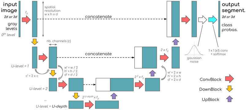
FIGURE 1. Modular U-Net: a generalization of the U-Net architecture.
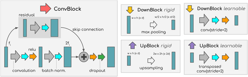
FIGURE 2. Examples of Modular U-Net blocks. Left: our Convolutional Block. Middle/right: rigid/learnable Down-sampling Block and Up-sampling Block.
In this paper, an annotated 3D XCT of glass fiber-reinforced Polyamide 66 (Figure 3) is presented as an example of segmentation problem in Materials Science that can be automated with a deep learning approach. Like Furat et al. (2019), we compare three variants on the composite material dataset focusing on the dimensionality of the convolutions (2D or 3D), obtaining qualitatively human-like segmentation (Figures 4–6) with all of them although 2D-convolutions yield better results (Figure 8). We find that (for the considered material) the U-Net architecture can be shallow without loss of performance, but batch normalization is necessary for the optimization (Figure 9). Finally, a learning curve (Figure 10) shows that only ten annotated 2D slices are necessary to train our model.
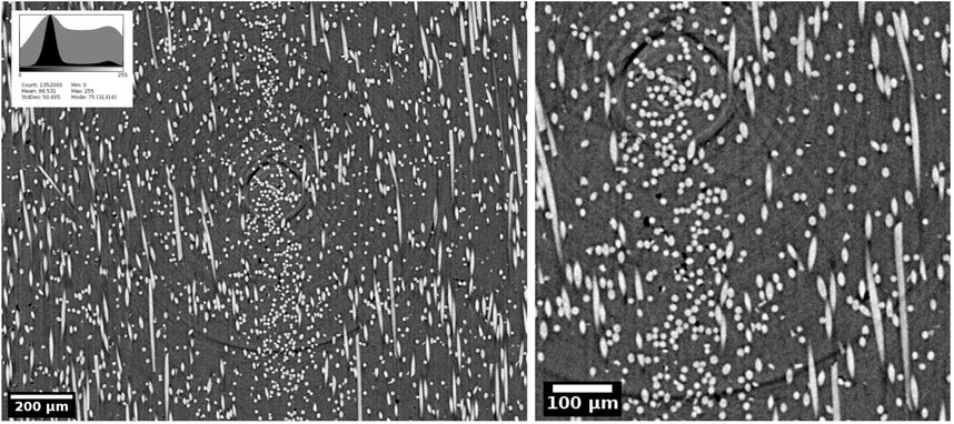
FIGURE 3. Glass fiber-reinforced Polyamide 66 tomography. Left: A 1300 × 1040 slice on the XY plane of the volume Train-Val-Test. In the upper left corner, a histogram of the gray level values in the image (linear scale in black, log scale in gray). Right: Zoom. Ring artifacts—from the acquisition process—can be as dark as porosities, making it harder to segment such regions.

FIGURE 4. Segmentation generated by the 2D model on the test set. Phase color code: blue represents voxels correctly classified as fiber (hatched), yellow as porosity (contours), and red represents misclassification. Notice that some regions in blue are in fact mistakenly segmented as fiber, although it is considered as correct because the annotations contain the same mistake. (B) is a zoom of the yellow-countoured area in (A).
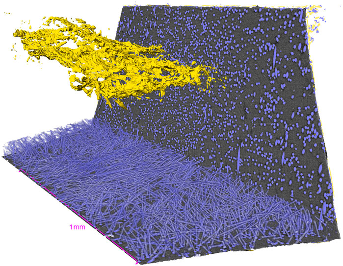
FIGURE 5. Segmentation generated by the 2D model on the volume Crack. Image rendered with standard tools in Avizo for the sake of visualization: two orthogonal planes inside the specimen, fibers rendered in 3D at the bottom, and the fracture rendered as a surface. Phase color code: blue represents the fiber and yellow represents the porosity.
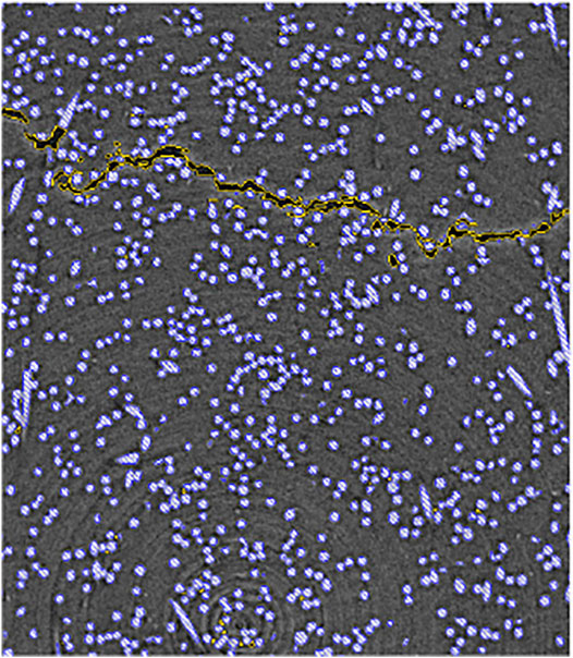
FIGURE 6. Segmentation of the volume Crack. A crop from the vertical plane in a slice passing through the fracture. The fiber phase is hatched in blue and the porosity phase is contoured in yellow.
Our results confirm that NNs can be not only a quality-wise satisfactory but also a viable solution in practice for XCT segmentation as it requires little annotated data and shallow models (therefore faster to train). Furthermore, the Modular U-Net, where the architecture becomes a set of hyperparameters, allows to optimize the model more easily and may ease the adoption of CNN-based models for automated X-ray tomography segmentation tasks.
2 Materials and Methods
2.1 Data
The data used in this work is composed of synchrotron X-ray tomography volumes recorded using 2 mm × 2 mm cross section composite specimens of Polyamide 66 reinforced by glass fibers, a material commonly used for structural pieces in different applications. XCT allows to assess the relation between the microstructure and the mechanical properties such as the resistance to the formation of damage under load. For this matter, segmenting such images automatically would, for instance, make it possible to visualize the propagation of cracks inside a specimen.
Two volumetric images (of different specimen) were used in this study. First, a volume of 20483 voxels, referred to as Train-Val-Test (Figure 3, 4), was cropped to get rid of the specimen’s borders, and its ground truth segmentation was created semi-manually with ImageJ (Schneider et al., 2012) using Fiji (Schindelin et al., 2012) and Avizo. Second, another specimen containing a fracture was segmented in order to qualitatively evaluate our models (Figures 5, 6)—it is further referred to as “Crack”—on a representative application of interest. All the data used in this work is publicly available; Table 1 describes the files published on Zeonodo (Bertoldo et al., 2021a).
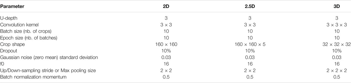
TABLE 1. Default hyperparameters. Parameters not mentioned are the default in TensorFlow 2.2.0.
2.1.1 Acquisition
X-ray tomography scans were recorded on the Psiché beamline at the Synchrotron SOLEIL using a parallel pink beam. The incident beam spectrum was characterized by a peak intensity at 25 keV, defined by the silver absorption edge, with a full width at half maximum bandwidth of approximately 1.8 keV. The total flux at the sample position was about 2.8e12 photons/s/mm2. The detector placed after the sample was constituted by a LuAG scintillator, a 5× magnifying optics, and a Hamamatsu CMOS 2048 × 2048 pixels detector (effective pixel size of 1.3 µm). 1,500 radiographs were collected over a 180° rotation and an exposure of 50 ms (full scan duration of 2 min). The sets of radiographs were then processed using PyHST2 reconstruction software (Mirone et al., 2014) with the Paganin filter (Paganin et al., 2002) activated to enhance the contrast between the phases.
2.1.2 Phases
The three phases in the material are visible in Figures 3, 4: the polymer matrix (gray), the glass fibers (white, hatched in blue), and damage in form of pores (dark gray and black, contoured in yellow). Although the pores (absence of material) do not constitute a real phase, they can be thought of as such for the sake of this study, and will be referred as porosity. Furthermore, a segmentation can be seen as a voxel-wise classification so the phases here are also referred to as “classes.”
2.1.3 Ground Truth
The data was annotated in two steps: first, the fiber and the porosity phases were independently segmented using Seeded Region Growing (Adams and Bischof, 1994); then, ring artifacts that leaked to the porosity class were manually corrected. A detailed description of the procedure is presented in the Supplementary Material.
2.1.4 Data Split
The ground truth tomography slices (of the Train-Val-Test volume) were sequentially split—their order was preserved to train the 3D models (Section 2.2.2)—into three sets: train (1300 slices), validation (128 slices), and test (300 slices). A margin of 86 slices between these sets was adopted to avoid information leakage. The “train” range was used to train the models, the “validation”) (or “val”) was used to select the best model (during the optimization), and the “test” was used to evaluate the models (Section 3).
2.1.5 Class Imbalance
Due to the material’s nature, the classes (phases) in this dataset are intrinsically imbalanced. The matrix, the fiber, and the porosity represent, respectively, 82.3, 17.2, and 0.5% of the voxels.
2.2 Neural Network
Let
In this section, a generic U-Net architecture, which we coined Modular U-Net (Figure 1), is proposed. We explain how it is composed and describe the modules used in this work. Three variants of the Modular U-Net were considered; their differences—based on the input, convolution, and output nature (2D or 3D)—are then analyzed (summary in Table 2). Finally, our training setup is described, specifying the loss function, optimizer, learning rate, data augmentation, software, and hardware used.
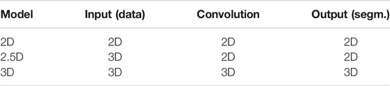
TABLE 2. Modular U-Net variations: input, convolutional layer, and output nature (2D or 3D).
2.2.1 Modular U-Net
Since Ronneberger et al. (2015) proposed U-Net, variations of it emerged in the literature [e.g., Çiçek et al. (2016); Qin et al. (2020)]. Here we propose a generalized version, preserving its overall structure. The Modular U-Net is based on three blocks (Figure 2): the Convolutional Block (ConvBlock), the Down-sampling Block (DownBlock), and the Up-sampling Block (UpBlock).
The left/right side of the architecture corresponds to an encoder/decoder: a repetition of pairs of ConvBlock and DownBlock/UpBlock modules. The two sides are connected by concatenations between their respective parts at the same U-level—which corresponds to the inner tensors’ resolutions (higher U-level means lower resolution). The U-depth, a hyperparameter, is the number of U-levels in a model, corresponding to the number of DownBlock (and equivalently UpBlock) modules.
The ConvBlock is a combination of operations that outputs a tensor with the same spatial dimensions of its input, though the number of channels may differ—in our models it always doubles. The assumption of equally-sized input/output is optional, but we admit it for the sake of simplicity because it makes the model easier to be used with an arbitrarily shaped volume. The number of channels after the ConvBlocks is 2U−level × f0, where f0 is the number of filters in the first convolution.
The DownBlock/UpBlock applies a down/up-sampling operation—which can be a learnable convolution/transposed convolution or a “rigid” max pooling/up-sampling (see Figure 2)—changing the tensor’s shape by dividing/multipling by two every spatial dimension: width, length, and depth in the 3D case. In other words, a tensor with shape (w, h, d, c)—where w, h, and d are the dimensions of the volume (respectively, the width, height, and depth), and c is the number of channels—becomes
In Ronneberger et al. (2015), for instance, the ConvBlock is a sequence of two 3 × 3 convolutions with ReLU activation, the DownBlock is a max pooling, and the UpBlock is an up-sampling layer. In Çiçek et al. (2016), the ConvBlock is a 3D convolutional layer, and in Qin et al. (2020) it is a nested U-Net.
The ConvBlock used here (Figure 2) is a sequence of two 3 × 3 (x3 in the 3D case) convolutions with ReLU activation, a residual connection with another convolution, batch normalization before each activation, and dropout at the end. The DownBlock is a 3 × 3 convolution with 2 × 2 stride, and the UpBlock is a 3 × 3 transposed convolution with 2 × 2 stride.
2.2.2 Variations: 2D, 2.5D, and 3D
Since our dataset contains intrinsically 3D structures, we compared the performances of this architecture using 2D and 3D convolutions. The 2D model processes individual tomography slices independently, while the 3D one processes several at once (i.e. a volume). We also compared an intermediate version, which we coined 2.5D; it processes one tomography slice at a time with 2D convolutions taking five consecutive slices at the input (the processed slice plus two above and two below), as if the extra slices were channels of a 2D image.
The 2D and 2.5D models can only process each slice of a plane individually; the XY plane (slices in the z-axis, as in Figures 3, 4) was chosen because the visual characteristics in this direction are mostly invariant—we observed a high correlation between adjacent slices.
These three variants have different receptive fields (therefore access to different information) and mix up the input entries differently (Table 2 summarizes these differences). The 2.5D model has access to extra information relative to the 2D model; its first convolution layer can correlate local information from adjacent tomography slices, although the rest of the network is identical in terms of structure. Meanwhile, the 3D model uses information from adjacent slices in every network layer, enabling more complex correlations but also increasing the model’s variance.
2.2.3 Training
The next paragraphs describe how our models were trained; Table 1 summarizes the hyperparameters of our neural network.
2.2.3.1 Loss Function
Our models were trained using a custom loss inspired on the Jaccard index, also known as Intersection over Union (IoU).
DEF. 1. Let A and B be two sets, and |⋅| denote a set’s cardinality. The Jaccard index J ∈ [0, 1] is
Similar to Duque-Arias et al. (2021), we adapt the right hand side of Eq. 1 to define the multi-class Jaccard2 loss for a batch of images.
For the sake of simplicity, the spatial dimensions (see Section 2.2) are omitted, and a single index n refers to position of individual voxels in a batch. In other words, instead of referring to a batch of normalized 3D images in [0, 1]w×h×d×b, where b is the batch size, we refer to an unraveled batch of voxels in [0, 1]N, where N = w × h × d × b. Nevertheless, the 3D structure remains implicitly unchanged—notice that the definition below remains the same for 2D images.
DEF. 2. Let y ∈ {0,1}N×C be a batch of ground truth voxels, where N is the number of voxels, each belonging to one out of C classes, such that
where yn is the voxel at position n ∈ [[N]], and yn,c is its cth entry (c ∈ [[C]]).
A model’s last activation map, a per-voxel softmax, is a tensor
The Jaccard2 loss of the batch
where
Notice that J2 ∈ (0, 1), thus it can, conveniently, be expressed as a percentage, and it is a measure of dissimilarity—J2 = 100% is a completely uncorrelated estimation, and J2 = 0% is a perfect replication of the ground truth—while Eq. 1 measures the similarity between two sets.
2.2.3.2 Data Augmentation
In order to increase the variability of the data, random crops were selected from the data volume, then a random geometric transformation (flip, 90° rotation, transposition, etc) is applied. As our training dataset is reasonably large, we used a simple data augmentation scheme, but richer transformations could be applied as long as the transformations result in credible samples.
2.2.3.3 Optimization
We used AdaBelief, an optimizer that combines the training stability and fast convergence of adaptive optimizers [e.g., Adam (Kingma and Ba, 2015)1] and good generalization capabilities of accelerated schemes (e.g., stochastic gradient descent).
Each model was trained for 200 epochs, each with 10 batches of 10 crops. The learning rate is set to 10−3 during the first 100 epochs then linearly decays until 10−4 during the last 100 epochs. This is done to quickly converge in the initial phase, then stabilize the optimization once it’s close to convergence. We verified that 200 epochs was enough to achieve convergence for all the models (the validation loss plateaus, oscilating randomly), and select the model with the lowest loss (i.e., not necessarily the one from the last epoch).
2.2.3.4 Software and Hardware
We trained our models using Keras with TensorFlow’s (Abadi et al., 2015) GPU-enabled version with CUDA 10.1 running on two NVIDIA Quadro P40002 (2 × 8 GN).
3 Results
In this section we present a compilation of qualitative and quantitative results obtained. The training process took one to 3 h for each model, up to 8 h for the largest 3D model. The segmentations from the three Modular U-Net versions presented in Section 2.2 are quantitatively compared, then an ablation analysis and the learning curve of the 2D model are presented. All the quantitative analyses were made on the test split (see Section 2.1), which contains 1300 × 1040 × 300 ≈ 406×106 voxels. The trained models and the data used to produce our results are publicly available online (Bertoldo et al., 2021a,b). A further detailed analysis is provided as Supplementary Material.
3.1 Qualitative Results
Figure 4 shows two snapshots of the volume Train-Val-Test in the test partition with a superposed segmentation generated with the 2D model. The zoomed area illustrates examples of misclassified regions—including parts of data with annotation mistakes.
The volume Crack was used to evaluate our method’s usability with another image (i.e., a volume from another specimen of the same material); the segmentation obtained with the 2D model is presented in Figures 5, 6. In terms of processing speed, the results show that our method could be carried out almost in real time using typical hardware available at a synchrotron beamline: using an NVIDIA Quadro P2000 (5 GB), it took 32 min to process the volume Crack, with approximately 5.8 billion voxels (1579 × 1845 × 2002).
3.2 Baseline
For the sake of comparison, we considered two theoretical models: the Zeroth Order Classifier (ZeroOC) and the Bin-wise ZeroOC. Both are described below, and their expected performances are summarized in Table 3. This analysis shows us the minimum expected Jaccard index for each class (see Table 3); notably, the mean class-wise Jaccard index of the Bin-wise ZeroOC is 76.2%.
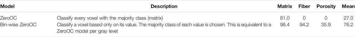
TABLE 3. Expected performance of baseline theoretical models in terms of class-wise Jaccard index (%).
The ZeroOC is the simplest model possible: it classifies every voxel with the majority class (the matrix phase), ignoring all the information from the data.
The Bin-wise ZeroOC takes gray level values into consideration individually (ignoring its neighbors) relying on the class imbalance on a per-value basis. Figure 7, the histograms of gray level value per class, illustrates this model’s principle: for a given gray level value in the x-axis, it selects the respective class of the highest curve in the y-axis—in other words, it always chooses the majority class conditioned on a given the gray level. The Bin-wise ZeroOC can be seen as a look-up table of gray level values as input and class as output, completely ignoring the contextual information available (the neighbor voxels).
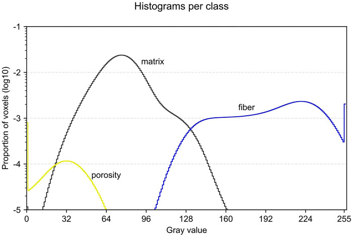
FIGURE 7. Glass fiber-reinforced Polyamide 66 gray value (normalized) histograms (one per class). The histogram is normalized globally, i.e., a bin’s value is the proportion of voxels out of all the voxels (all classes confounded). The superposition of the classes’ value ranges make it impossible to segment the image with a threshold on the gray values.
3.3 Quantitative Results
Figure 8 presents a comparison of the three model variations (2D, 2.5D, and 3D), where they are evaluated with varying sizes. The models are scaled with the hyperparameter f0 (values inside the parentheses in Figure 8).
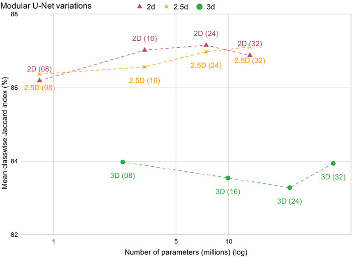
FIGURE 8. Modular U-Net variations comparison. On the x-axis, the number of parameters; on the y-axis the mean class-wise Jaccard indices. The Modular U-Net 2D, 2.5D, and 3D versions are scaled with f0 (in parentheses), the number of filters of the first convolution of the first Convolutional Block.
The performance is measured using the Jaccard index, also known as Intersection over Union (IoU), on each phase (class). Our main metric is the arithmetic mean of the three class-wise indices, and the baseline minimum is 76.2%, Bin-wise ZeroOC’s performance. This metric provides a good visibility of the performance differences and resumes the precision-recall trade off; other classic metrics—even the area under the Receiver Operating Characteristic (ROC) curve (Hanley and McNeil, 1982)—are close to 100% (see the Supplementary Material), so the differences are hard to compare.
3.4 Ablation Study
Figure 9 presents a component ablation analysis of the 2D model with f0 = 16 in terms of number of parameters and performance. Starting with the 2D model with the default hyperparameters (see Figure 2; Table 1), we retrained other models removing one component at a time. The learnable up/down-samplings were replaced by “rigid” ones (see Figure 2), the 2D convolutions were replaced by separable ones, and the batch normalization was replaced by layer normalization. Finally, we varied the U-depth from 2 to 4.
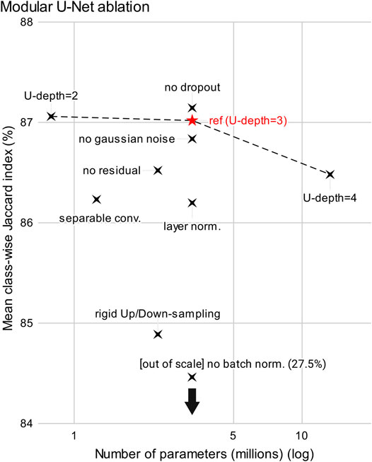
FIGURE 9. Modular U-Net ablation (2D model). On the x-axis, the number of parameters; on the y-axis the mean class-wise Jaccard indices. Components were removed individually, or replaced by alternatives. Removals: dropout, gaussian noise, residual (skip connection), batch normalization. Replacements: convolutions by separable ones, learnable Down-sampling Block/Up-sampling Block by rigid ones (Figure 2), and batch normalization by layer normalization. We also compare the effect of the U-depth, i.e., number of levels in the U structure. Notice that the data point no batch norm is out of scale in the y-axis for the sake of visualization.
Notice that the model without dropout performed better than the reference model, but we kept it in our default parameters because the same thing did not occur with other variations and sizes.
3.5 Learning Curve
Finally, we computed the learning curve of the 2D model in order to assess the trade-off between performance and amount of annotated data. As the data annotation is time-consuming and requires expertise (therefore expensive), this analysis intends to estimate how much annotation is necessary to achieve our results. The number of (consecutive) slices in the training dataset was progressively decreased from 1024 to 1 while the validation dataset is kept the same (300 slices) for evaluation. This experiment was run with the 2D Modular U-Net using the default hyperparameters (presented in Table 1), and the results presented in Figure 10 in terms of class-wise Jaccard index and their arithmetic mean.
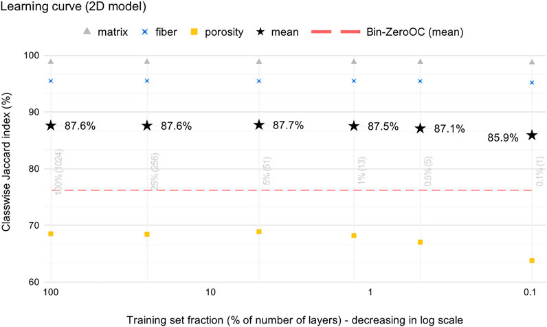
FIGURE 10. Learning curve of the 2D model with default hyperparameters (Table 1). 1024 consecutive slices from the training set were used with progressively fewer data by eliminating slices from the bottom (i.e., closer to the validation set, see Section 2.1.4) of the stack. All the models are evaluated with the validation set.
4 Discussions
4.1 Overview
Our models achieved, qualitatively, very satisfactory results from a Materials Science application point of view, with 87% of mean class-wise Jaccard index and an F1-score macro average of 92.4% (Supplementary Material). We stress the fact that these results were achieved without any strategy to compensate the (heavy) class imbalance (82.3% of the voxels belong to the class matrix); they may be further improved using, for instance, re-sampling strategies (Ando and Huang, 2017; Pouyanfar et al., 2018), class-balanced loss functions (Cao et al., 2019; Khan et al., 2019), or self-supervised pre-training (Yang and Xu, 2020).
The results obtained with another specimen (the Crack volume), thus with slight variations in the acquisition conditions, were way faster than the manual process while keeping good quality—inspection by an expert showed no relevant error in the segmentation as compared to a human-made one. The fracture was mostly, and correctly, segmented as porosity without retraining the model, showing its capacity to generalize—an important feature for its practical use, although some misclassified regions can be seen as holes (missing pieces) in the fracture’s surface (Figure 5).
Moreover, the processing time achieved (32 min) is indeed a promising prospect compared to classic approaches.
4.2 Segmentation Errors
As highlighted in Figure 4, the 2D model’s mistakes (in red), are mostly on the interfaces of the phases, which are fairly comparable to a human annotator’s. We (informally) estimate that they are in the error margin because, in some regions, there is no clear definition of the phases’ limits. The fibers may show smooth, blurred phase boundaries with the matrix, while some pores are smaller than the image resolution.
Another issue is the loss of information (all-zero regions) in some rings (e.g., Figure 3). In such cases, even though one could deduce that there is indeed a pore, it is practically impossible to draw a well-defined interface.
Finally, we reiterate that the ground truth remains slightly imperfect despite our efforts to mitigate these issues. For instance, in Figure 4 we see, inside the C-like shaped porosity, a blue region, meaning that it was “correctly” segmented as a fiber—yet, there is no fiber in it.
4.3 Model Variations
Figure 10 confirms that the porosity class is harder to detect. Although, the qualitative results are reasonable, and we underline that the Jaccard index is more sensitive on underrepresented classes because the size of the union will always be smaller (see Equations in the Supplementary Material).
Contrarily to our expectations, Figure 8 shows that the 2D model performed systematically better than the 3D (albeit the difference is admittedly small). We expected the 3D model to perform better because the morphology of the objects in the image are naturally three-dimensional; besides, other work (Furat et al., 2019) have obtained better results in binary segmentation problems. We raise three hypotheses about this result: 1) the set of hyperparameters is not optimal, 2) the performance metric is biased because the annotation process uses a 2D algorithm, and 3) the 3D models suffer more from overfitting because they have higher variance (more parameters, see Figure 8).
4.4 Model Ablation
Figure 9 contains a few interesting findings about the hyperparameters of the Modular U-Net:
1. using learnable up/down-sampling operations indeed gives more flexibility to the model, improving its performance compared to “rigid” (not learnable) operations;
2. separable convolutions slightly hurt the performance, but it reduces the number of parameters by 60%;
3. decreasing the U-depth, therefore shrinking the receptive field, improved the performance while reducing 75% of the model size; on the other hand, increasing the depth had the opposite effect, multiplying the model size by four, while degrading the performance;
4. batch normalization is essential for the training—notice that the version without batch normalization is out of scale in Figure 9, and its performance corresponds to the ZeroOC model (see the Supplementary Material);
Model depth (item 3): this finding gives a valuable information for our future work because using shallower models require less memory (i.e., bigger crops can be processed at once), making it possible to accelerate the processing time. We hypothesize that the necessary receptive field for image segmentation is smaller than the model with U-depth three. Therefore, a spatially bigger input captures irrelevant, spurious context to the classification.
4.5 Learning Curve
Figure 10 highlights a very promising finding in our results: very little annotation is necessary to train a reasonable model. The 2D Modular U-Net was capable of learning with only 1% of the train dataset (13 z-slices) without any smart strategy to select the slices (i.e., one could pick sparsely separated slices to achieve more data variability).
Furthermore, even a single slice was sufficient to achieve a reasonable performance. Notice that the Jaccard index of the porosity is still much higher than its baseline even though this class represents 0.5% of the voxels. On the other hand, this is possibly because it is an “easier” class, as its gray level values are concetrated around zero (see Figure 7).
This result is of great interest from an application point of view because the annotation process is an important bottleneck to take our method to a practical application. Notice that the data was semi-automatically annotated with other algorithms (Seeded Region Growing and adhoc standard image transformations) and still contain imperfections (e.g., Figure 4), so the results can improve with a more refined methodology. In other words, Figure 10 tells us that one could obtain a preliminary segmentation by annotating a single slice of this material, then iterate by refining the model’s results in order to obtain a few tens of slices, which would provide usable results.
5 Conclusion
A dataset of XCT images of glass fiber-reinforced Polyamide 66, a three-phase composite material, was presented and segmented with U-Nets; requiring the annotation of only a few tomography slices, results show a promising venue to automate processing pipelines for synchrotron XCT.
We proposed the Modular U-Net, a reinterpretation of its precursor that provides a more abstract, conceptually more compact representation of this family of neural network architectures by identifying three essential blocks of a U-Net. As many variations of U-Net have been presented in the literature, we expect this re-description of the model to facilitate the communication of their implementation details. Three variants of the Modular U-Net (2D, 2.5D, and 3D) were compared, showing that all three were capable of learning the patterns from a human-made annotation, although the 2D version performed better than the others.
An ablation study of the 2D Modular U-Net provided insights about its components revealing that we might further accelerate the processing with smaller models, and its learning curve revealed that only 13 annotated slices are necessary to achieve our results—in addition, a single slice was sufficient to obtain preliminary results. Finally, we note that further improvements could be achieved by adding other techniques on top of our work, for instance refining the annotations, compensating the data imbalance, and using more advanced architectures like UNet++ (Zhou et al., 2018), which adds new, more complex, skip connections to U-Net.
Data Availability Statement
The datasets presented in this study can be found in an online repository (Bertoldo et al., 2021a). The names of the files and their respective volumes mentioned here are summarized in Table 4.
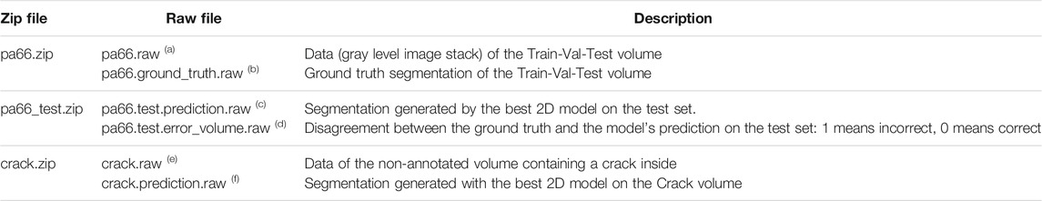
TABLE 4. Published 3D volumes: all the data necessary to train and test the models presented in this paper are publicly available on Zenodo (Bertoldo et al., 2021a). The raw files have complementary raw.info files containing metadata (volume dimensions and data type) about its respective volume. Notice that the volumes (a) and (b) contain all the three splits (train, validation, test) together (1900 z-slices), while the volumes (c) and (d) correspond to their last 300 z-slices. A demo of how to read the data is available on GitHub. The values in the data volumes are integers from 0 to 255, where the former is black and the latter is white. The values in the segmentation volumes (predictions and ground truth) are 0, 1, and 2, which respectively correspond to the phases matrix, fiber, and porosity. The volumes (e) and (f) correspond to the volume in Figures 5, 6. Figure 3 was generated in Fiji (Schindelin et al., 2012) with the volume (a). Figure 4 was generated in Avizo with volumes (a) and (d), which is derived from volumes (b) and (c). Figure 6 was generated in Avizo with volumes (e) and (f).
Author Contributions
JPCB conducted the experiments and wrote this manuscript. ED assisted the code development, helped design the experiment, and reviewed this manuscript. DR reviewed this manuscript. HP acquired the data, helped design the experiment, and reviewed this manuscript.
Funding
JPCB was funded by the BIGMÉCA research initiative (ttps://bigmeca.minesparis.psl.eu), funded by Safran and MINES ParisTech.
Conflict of Interest
The authors declare that the research was conducted in the absence of any commercial or financial relationships that could be construed as a potential conflict of interest.
Publisher’s Note
All claims expressed in this article are solely those of the authors and do not necessarily represent those of their affiliated organizations, or those of the publisher, the editors and the reviewers. Any product that may be evaluated in this article, or claim that may be made by its manufacturer, is not guaranteed or endorsed by the publisher.
Acknowledgments
JB would like to thank the funding from the BIGMÉCA. HP would like to acknowledge beam time allocation at the Psiché beamline of Synchrotron SOLEIL for the proposal number 20150371.
Supplementary Material
The Supplementary Material for this article can be found online at: https://www.frontiersin.org/articles/10.3389/fmats.2021.761229/full#supplementary-material
Footnotes
1Adam yielded equivalent results but took longer (more epochs) to converge
References
Abadi, M., Agarwal, A., Barham, P., Brevdo, E., Chen, Z., Citro, C., et al. (2015). TensorFlow: Large-Scale Machine Learning on Heterogeneous Systems. Savannah, GA: USENIX Association.
Adams, R., and Bischof, L. (1994). Seeded Region Growing. IEEE Trans. Pattern Anal. Machine Intell. 16, 641–647. doi:10.1109/34.295913
Ando, S., and Huang, C. Y. (2017). “Deep Over-sampling Framework for Classifying Imbalanced Data,” in Machine Learning and Knowledge Discovery in Databases. Editors M. Ceci, J. Hollmén, L. Todorovski, C. Vens, and S. Džeroski (Cham: Springer International Publishing), 770–785. doi:10.1007/978-3-319-71249-9_46
Badrinarayanan, V., Kendall, A., and Cipolla, R. (2017). SegNet: A Deep Convolutional Encoder-Decoder Architecture for Image Segmentation. IEEE Trans. Pattern Anal. Mach. Intell. 39, 2481–2495. doi:10.1109/TPAMI.2016.2644615
Bengio, Y., and Lecun, Y. (1997). Convolutional Networks for Images, Speech, and Time-Series. Available at: https://dl.acm.org/doi/10.5555/303568.303704
Bertoldo, J., Decencière, E., Ryckelynck, D., and Proudhon, H. (2021a). Glass Fiber-Reinforced Polyamide 66 3d X-ray Computed Tomography Dataset for Deep Learning Segmentation. [Dataset]. doi:10.5281/zenodo.4587827
Bertoldo, J., Decencière, E., Ryckelynck, D., and Proudhon, H. (2021b). Glass Fiber-Reinforced Polyamide 66 3d X-ray Computed Tomography Segmentation Segmentation U-Nets. [Dataset]. doi:10.5281/zenodo.4601560
Beucher, S. (1994). “Watershed, Hierarchical Segmentation and waterfall Algorithm,” in Morphology and its Applications to Image Processing. (Dordrecht: Springer), 2, 69–76. doi:10.1007/978-94-011-1040-2_10
Cao, K., Wei, C., Gaidon, A., Aréchiga, N., and Ma, T. (2019). “Learning Imbalanced Datasets with Label-Distribution-Aware Margin Loss,” in Advances in Neural Information Processing Systems 32: Annual Conference on Neural Information Processing Systems 2019, NeurIPS 2019, Vancouver, BC, Canada, December 8-14, 2019. Editors H. M. Wallach, H. Larochelle, A. Beygelzimer, F. d’Alché Buc, E. B. Fox, and R. Garnett, 1565–1576.
Çiçek, Ö., Abdulkadir, A., Lienkamp, S., Brox, T., and Ronneberger, O. (2016). “3D U-Net: Learning Dense Volumetric Segmentation from Sparse Annotation,” in Medical Image Computing and Computer-Assisted Intervention (MICCAI). (Cham, Switzerland: Springer International Publishing). doi:10.1007/978-3-319-46723-8_49
Duque-Arias, D., Velasco-Forero, S., Deschaud, J.-E., Goulette, F., Serna, A., Decencière, E., et al. (2021). “On Power Jaccard Losses for Semantic Segmentation,” in VISAPP 2021: 16th International Conference on Computer Vision Theory and Applications, Vienne (on line), Austria, February 2021. doi:10.5220/0010304005610568
Furat, O., Wang, M., Neumann, M., Petrich, L., Weber, M., Krill III, C. E., et al. (2019). Machine Learning Techniques for the Segmentation of Tomographic Image Data of Functional Materials. Front. Mater. 6, 145. doi:10.3389/fmats.2019.00145
Hanley, J. A., and McNeil, B. J. (1982). The Meaning and Use of the Area under a Receiver Operating Characteristic (ROC) Curve. Radiology 143, 29–36. doi:10.1148/radiology.143.1.7063747
Khan, S., Hayat, M., Zamir, S. W., Shen, J., and Shao, L. (2019). “Striking the Right Balance with Uncertainty,” in 2019 IEEE/CVF Conference on Computer Vision and Pattern Recognition (CVPR), Long Beach, CA, June 2019, 103–112. doi:10.1109/cvpr.2019.00019
Kingma, D. P., and Ba, J. (2015). “Adam: A Method for Stochastic Optimization,” in 3rd International Conference on Learning Representations, ICLR 2015, San Diego, CA, USA, May 7-9, 2015. Editors Y. Bengio, and Y. LeCun.
Maire, E., Le Bourlot, C., Adrien, J., Mortensen, A., and Mokso, R. (2016). 20 Hz X-ray Tomography during an In Situ Tensile Test. Int. J. Fract. 200, 3–12. doi:10.1007/s10704-016-0077-y
Maire, E., and Withers, P. J. (2014). Quantitative X-ray Tomography. Int. Mater. Rev. 59, 1–43. doi:10.1179/1743280413Y.0000000023
Mirone, A., Brun, E., Gouillart, E., Tafforeau, P., and Kieffer, J. (2014). The PyHST2 Hybrid Distributed Code for High Speed Tomographic Reconstruction with Iterative Reconstruction and A Priori Knowledge Capabilities. Nucl. Instr. Methods Phys. Res. Section B: Beam Interactions Mater. Atoms 324, 41–48. doi:10.1016/j.nimb.2013.09.030
Oktay, O., Schlemper, J., Folgoc, L. L., Lee, M., Heinrich, M., Misawa, K., et al. (2018). Attention U-Net: Learning where to Look for the Pancreas. arXiv. arXiv:1804.03999 [cs] [Preprint].
Pacchioni, G. (2019). An Upgrade to a Bright Future. Nat. Rev. Phys. 1, 100–101. doi:10.1038/s42254-019-0019-5
Paganin, D., Mayo, S. C., Gureyev, T. E., Miller, P. R., and Wilkins, S. W. (2002). Simultaneous Phase and Amplitude Extraction from a Single Defocused Image of a Homogeneous Object. J. Microsc. 206, 33–40. doi:10.1046/j.1365-2818.2002.01010.x
Pouyanfar, S., Tao, Y., Mohan, A., Tian, H., Kaseb, A. S., Gauen, K., et al. (2018). “Dynamic Sampling in Convolutional Neural Networks for Imbalanced Data Classification,” in 2018 IEEE Conference on Multimedia Information Processing and Retrieval (MIPR), Miami, Florida, April, 2018, 112–117. doi:10.1109/MIPR.2018.00027
Qin, X., Zhang, Z., Huang, C., Dehghan, M., Zaiane, O. R., and Jagersand, M. (2020). U2-Net: Going Deeper with Nested U-Structure for Salient Object Detection. Pattern Recognit. 106, 107404. doi:10.1016/j.patcog.2020.107404
Ronneberger, O., Fischer, P., and Brox, T. (2015). “U-net: Convolutional Networks for Biomedical Image Segmentation,” in Medical Image Computing and Computer-Assisted Intervention. Editors N. Navab, J. Hornegger, W. M. Wells, and A. F. Frangi (Cham: Springer International Publishing), 234–241. doi:10.1007/978-3-319-24574-4_28
Rosenblatt, F. (1958). The Perceptron: a Probabilistic Model for Information Storage and Organization in the Brain. Psychol. Rev. 65 (6), 386–408. doi:10.1037/h0042519
Schindelin, J., Arganda-Carreras, I., Frise, E., Kaynig, V., Longair, M., Pietzsch, T., et al. (2012). Fiji: An Open-Source Platform for Biological-Image Analysis. Nat. Methods 9, 676–682. doi:10.1038/nmeth.2019
Schneider, C. A., Rasband, W. S., and Eliceiri, K. W. (2012). NIH Image to ImageJ: 25 Years of Image Analysis. Nat. Methods 9, 671–675. doi:10.1038/nmeth.2089
Shashank Kaira, C., Yang, X., De Andrade, V., De Carlo, F., Scullin, W., Gursoy, D., et al. (2018). Automated Correlative Segmentation of Large Transmission X-ray Microscopy (TXM) Tomograms Using Deep Learning. Mater. Charact. 142, 203–210. doi:10.1016/j.matchar.2018.05.053
Shelhamer, E., Long, J., and Darrell, T. (2017). Fully Convolutional Networks for Semantic Segmentation. IEEE Trans. Pattern Anal. Mach. Intell. 39, 640–651. doi:10.1109/tpami.2016.2572683
Shuai, S., Guo, E., Phillion, A. B., Callaghan, M. D., Jing, T., and Lee, P. D. (2016). Fast Synchrotron X-ray Tomographic Quantification of Dendrite Evolution during the Solidification of Mg Sn Alloys. Acta Material. 118, 260–269. doi:10.1016/j.actamat.2016.07.047
Stan, T., Thompson, Z. T., and Voorhees, P. W. (2020). Optimizing Convolutional Neural Networks to Perform Semantic Segmentation on Large Materials Imaging Datasets: X-ray Tomography and Serial Sectioning. Mater. Charact. 160, 110119. doi:10.1016/j.matchar.2020.110119
Stoller, D., Ewert, S., and Dixon, S. (2018). “Wave-U-Net: A Multi-Scale Neural Network for End-To-End Audio Source Separation,” in Proceedings of the 19th International Society for Music Information Retrieval Conference (ISMIR 2018), Calgary, AB, April, 2018.
Strohmann, T., Bugelnig, K., Breitbarth, E., Wilde, F., Steffens, T., Germann, H., et al. (2019). Semantic Segmentation of Synchrotron Tomography of Multiphase Al-Si Alloys Using a Convolutional Neural Network with a Pixel-wise Weighted Loss Function. Sci. Rep. 9, 1–9. doi:10.1038/s41598-019-56008-7
Withers, P. J., Bouman, C., Carmignato, S., Cnudde, V., Grimaldi, D., Hagen, C. K., et al. (2021). X-Ray Computed Tomography. Nat. Rev. Methods Primers 1, 1–21. doi:10.1038/s43586-021-00015-4
Yang, Y., and Xu, Z. (2020). “Rethinking the Value of Labels for Improving Class-Imbalanced Learning,” in Advances in Neural Information Processing Systems. Editors H. Larochelle, M. Ranzato, R. Hadsell, M. F. Balcan, and H. Lin (Curran Associates, Inc.), Vol. 33, 19290–19301. file:///Users/daniellehiraldo/Downloads/Best-Practices-AIAN-Data-Collection-20200826.pdf.
Zhang, Z., Liu, Q., and Wang, Y. (2018). Road Extraction by Deep Residual U-Net. IEEE Geosci. Remote Sensing Lett. 15, 749–753. doi:10.1109/lgrs.2018.2802944
Zhou, Z., Rahman Siddiquee, M. M., Tajbakhsh, N., and Liang, J. (2018). “UNet++: A Nested U-Net Architecture for Medical Image Segmentation,” in Deep Learning in Medical Image Analysis and Multimodal Learning for Clinical Decision Support. Editors D. Stoyanov, Z. Taylor, G. Carneiro, T. Syeda-Mahmood, A. Martel, L. Maier-Heinet al. (Cham: Springer International Publishing), 3–11. doi:10.1007/978-3-030-00889-5_1
Keywords: deep learning, U-net, modular network architecture, semantic segmentation, 3D X-ray computed tomography (XCT), composite material
Citation: Bertoldo JPC, Decencière E, Ryckelynck D and Proudhon H (2021) A Modular U-Net for Automated Segmentation of X-Ray Tomography Images in Composite Materials. Front. Mater. 8:761229. doi: 10.3389/fmats.2021.761229
Received: 19 August 2021; Accepted: 22 October 2021;
Published: 25 November 2021.
Edited by:
Zhenyu Li, University of Science and Technology of China, ChinaReviewed by:
Orkun Furat, University of Ulm, GermanyXiaojun Wu, University of Science and Technology of China, China
Copyright © 2021 Bertoldo, Decencière , Ryckelynck and Proudhon. This is an open-access article distributed under the terms of the Creative Commons Attribution License (CC BY). The use, distribution or reproduction in other forums is permitted, provided the original author(s) and the copyright owner(s) are credited and that the original publication in this journal is cited, in accordance with accepted academic practice. No use, distribution or reproduction is permitted which does not comply with these terms.
*Correspondence: João P. C. Bertoldo, am9hby5iZXJ0b2xkb0BtaW5lcy1wYXJpc3RlY2guZnI=