Efficient Fitting of 3D Tessellations to Curved Polycrystalline Grain Boundaries

The curvature of grain boundaries in polycrystalline materials is an important characteristic, since it plays a key role in phenomena like grain growth. However, most traditional tessellation models that are used for modeling the microstructure morphology of these materials, e.g., Voronoi or Laguerre tessellations, have flat faces and thus fail to incorporate the curvature of the latter. For this reason, we consider generalizations of Laguerre tessellations—variations of so-called generalized balanced power diagrams (GBPDs)—that exhibit non-convex cells. With as many as ten parameters for each cell, it is computationally demanding to fit GBPDs to three-dimensional image data containing hundreds of grains. We therefore propose a modification of the traditional definition of GBDPs that allows gradient-based optimization methods to be employed. The resulting reduction in runtime makes it feasible to find approximations to real experimental datasets. We demonstrate this on a three-dimensional x-ray diffraction (3DXRD) mapping of an AlCu alloy, but we also evaluate the modeling errors for simulated data. Furthermore, we investigate the effect of noisy image data and whether the smoothing of image data prior to the fitting step is advantageous.

1 Introduction

The grain boundaries of polycrystalline materials play an important role in many different phenomena, ranging from fundamental processes like grain growth and extending to applied scenarios like the degradation of electrodes in lithium-ion batteries. In many such cases, the investigation and modeling of grain boundaries presupposes that their locations can be represented precisely. For this purpose, tessellations have proven to be a powerful tool, as they provide a partitioning of space into disjoint subsets called cells. For example, the representation of a material’s microstructure by means of tessellations can be utilized for the analysis of microstructure-property relationships (Raabe, 1998; Westhoff et al., 2018). For the latter, realistic “virtual polycrystals” generated by parametric stochastic models for these tessellations are particularly helpful (see, e.g., Allen et al., 2021). A prominent tessellation type in materials science is the Laguerre tessellation (Lautensack and Zuyev, 2008), which is a generalization of the well-known Voronoi tessellation (Møller, 1994; Okabe et al., 2000). It is therefore not surprising that the fitting of Laguerre tessellations to experimental data has already received much attention. For example, in Bourne et al. (2020); Petrich et al. (2019); Quey and Renversade (2018) the problem of finding good representations for statistical data, such as grain volumes and centroids, is discussed. Of particular interest is the description of 3D image data, e.g., from 3D electron backscatter diffraction (EBSD) or 3D x-ray diffraction (3DXRD) microscopy, which was studied in Liebscher (2015); Quey and Renversade (2018); Spettl et al. (2016). Additional details regarding the method proposed in Spettl et al. (2016) are given in Section 2.4.1. A major drawback of the Laguerre tessellation, however, is the fact that its facets are planar and therefore apply only to grains having nearly flat boundaries. This is unacceptable when it comes to the investigation of curvature-related phenomena like grain growth. In this case, other tessellation models—often generalizations of the Voronoi/Laguerre tessellations—have been proposed; we refer to Altendorf et al. (2014); Šedivý et al. (2018) for an overview. Heuristics for fitting some of these tessellation models are described in Altendorf et al. (2014); Teferra and Graham-Brady (2015). A quite general tessellation model, the so-called generalized balanced power diagram (GBPD), is introduced in Alpers et al. (2015), in which a fitting procedure based on a (very high-dimensional) linear optimization is also proposed. A different fitting method, again relying on optimization, is described by Šedivý et al. (2016). Moreover, a completely different approach is taken in Teferra and Rowenhorst (2018), where closed formulas for approximating GBPDs are presented. The latter two methods are discussed in detail in Sections 2.4.2 and 4.2.

The major goal of the present paper is to propose a fitting method that works well for GBPDs and other distance-based tessellations. Taking advantage of efficient gradient-descent optimization, the new approach aims to achieve a goodness of fit similar or better than that of other techniques—but with much shorter computational runtime. This is investigated on 3DXRD mapping data obtained from a sample of an AlCu alloy, but we also evaluate the modeling errors for simulated data. Note that the fitting method presented here is also applicable to image data obtained by techniques other than 3DXRD, such as 3D EBSD (Zaefferer et al., 2008; Schwartz et al., 2009; Burnett et al., 2016). Furthermore, the robustness with respect to noisy image data is studied, and the question is posed whether the smoothing of grain boundaries prior to tessellation fitting—as is routinely carried out—actually improves the fit. Even though different tessellation models were fitted to the datasets, the topic of model selection is not discussed; for the latter, we refer to Šedivý et al. (2018). The present paper extends a previous version of the fitting algorithm originally described in Furat et al. (2021) by considering more general types of tessellations and a thorough analysis of the goodness of fit for different datasets.

2 Materials and Methods

In this section we describe the materials and methods used in the present paper. These topics include the 3DXRD image data described in Section 2.1, the definitions of various tessellation models in Section 2.2, a procedure for gradient descent-based tessellation fitting in Section 2.3 (originally introduced in Furat et al. (2021)), and two further methods from the literature for the gradient-free fitting of tessellations to image data (Section 2.4).

2.1 Description of 3DXRD Image Data

One of the main goals of the present paper is to describe a procedure for finding accurate parametric representations of real, experimental image data. To that end, a 3D microstructural mapping was carried out on a 1.4 mm-diameter cylinder of Al-5 wt%Cu, which was cut out of a cold-rolled plate (50% thickness reduction) that had been subsequently homogenized at 500°C for 24 h in air. The shape of individual grains in the specimen and the location of internal grain boundaries were revealed by 3DXRD microscopy measurements, performed at beamline BL20XU of the Japanese synchrotron radiation facility SPring-8 using a monochromatic beam of 32 keV x-rays (Poulsen, 2004). For 10 min prior to this room-temperature mapping, the specimen was subjected to a heat treatment at 575°C in air, which results in a liquid AlCu phase of approximately 2 vol% wetting the boundaries between the solid, aluminum-rich grains. Owing to the simultaneous presence of two phases, the resulting evolution of the sample’s microstructure is classified as Ostwald ripening (Wang and Glicksman, 2007). Once the sample is removed from the furnace, however, the liquid layer crystallizes and the growth/shrinkage of individual grains ceases.

Reconstruction of the 3DXRD data followed the protocol described in Dake et al. (2016), relying on the data processing routines of Schmidt (2005, 2014). To each voxel in the reconstructed volume, the software assigns the crystal lattice orientation that generates the most complete diffraction signal, whereby “completeness” is defined as the ratio between the number of experimentally detected diffraction spots associated with the voxel in question and the number of diffraction spots that are simulated to arise from this particular voxel if it were to have the assumed orientation. The grain labels were then assigned voxel-by-voxel to the orientation having the greatest completeness value. Formally, we describe the resulting image dataset as a mapping

$I_{\mathrm{E},\mathrm{r}\mathrm{a}\mathrm{w}}:{\mathcal{W}}_{\mathrm{E},\mathrm{r}\mathrm{a}\mathrm{w}}=\left\{1,\dots ,531\right\}\times \left\{1,\dots ,321\right\}\times \left\{1,\dots ,321\right\}\to \left\{0,\dots ,943\right\},$

where each voxel coordinate is mapped to the corresponding grain label. Here, the label 0 is assigned to the background (i.e., voxels located outside the specimen). Each of the remaining labels is associated with one of the 943 grains.

However, with this reconstruction procedure the grain boundaries may manifest irregularities, such as local roughness, “island” voxels, zigzag shapes, or regions of fluctuating curvature (see Figure 1A) as a result of measurement uncertainties. These artifacts can be eliminated by treating the raw reconstruction as the initial configuration of a computational simulation of curvature-driven grain growth. If the duration of such a simulation is kept short enough, any boundary location manifesting severe curvature will tend to smoothen out, and any island voxels will be consumed by the surrounding grain, but no long-range translation of boundaries will occur—see Figure 1B. In the present paper, we employed 25 iterations of a 3D phase field algorithm (Krill and Chen, 2002) to reduce the roughness of grain boundaries in the raw 3DXRD reconstructions. The resulting smoothed experimental image is referred to as

$I_{\mathrm{E},\mathrm{s}\mathrm{m}\mathrm{o}\mathrm{o}\mathrm{t}\mathrm{h}}:{\mathcal{W}}_{\mathrm{E},\mathrm{s}\mathrm{m}\mathrm{o}\mathrm{o}\mathrm{t}\mathrm{h}}\to \left\{0,\dots ,938\right\},$

where ${\mathcal{W}}_{\mathrm{E},\mathrm{s}\mathrm{m}\mathrm{o}\mathrm{o}\mathrm{t}\mathrm{h}}={\mathcal{W}}_{\mathrm{E},\mathrm{r}\mathrm{a}\mathrm{w}}$. Note that some smaller grains vanished during the data smoothing procedure; consequently, I_E,smooth had fewer grains than I_E,raw (938 grains instead of 943).

FIGURE 1

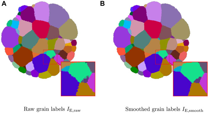
FIGURE 1. Two-dimensional slice through the raw (A) and smoothed (B) experimental 3D image data and a magnified region showing the grain boundaries.

2.2 Tessellation Models

In order to represent the 3D grain architecture of (measured and simulated) image data in an efficient way, we apply an optimization method to decompose the volume of interest into subvolumes using tessellations. Thus, to begin with, we briefly describe the tessellation models considered in the present paper. For additional details on tessellations in general, we refer, e.g., to Chiu et al. (2013).

Roughly speaking, a tessellation is a partitioning of space into pairwise disjoint sets, so-called cells. More precisely, a tessellation $\mathcal{T}$ in a sampling window $\mathcal{W}\subset {\mathbb{R}}^3$ is a countable collection of sets (cells), $\mathcal{T}=\{C_i^{\mathcal{T}}\subset \mathcal{W}:i=\mathrm{1,2},\dots \}$, such that

1) $\mathrm{int}(C_i^{\mathcal{T}})\cap \mathrm{int}(C_j^{\mathcal{T}})=\varnothing \text{\hspace{0.17em}for\hspace{0.17em}}i\ne j$,

2) ${\cup }_{i=1}^{\infty }{C}_i^{\mathcal{T}}=\mathcal{W}$,

3) and $\mathcal{T}$ is locally finite—i.e., $\#\{C^{\mathcal{T}}\in \mathcal{T}:C^{\mathcal{T}}\cap B\ne \varnothing \}<\infty$ for all bounded $B\subset \mathcal{W}$,

where int(⋅) denotes the interior of a set. Note that in this paper we consider tessellations only in a bounded sampling window $\mathcal{W}\subset {\mathbb{R}}^3$. In this case, the number of (non-empty) cells is finite and is denoted by $n_{\mathcal{T}}.$

For practical purposes, such as finding simplified representations of experimental image data, parametric tessellation models are probably the most suitable class of tessellations. The tessellation models considered in the present paper have in common that their cells are defined in terms of a distance function $d_{\mathcal{T}}:{\mathbb{R}}^3\times \mathbb{G}\to \mathbb{\{R\}}$, where {$\mathbb{G}$} denotes the domain of generators (i.e., a set of admissible parameters of a single tessellation cell). For a (finite) set of generators $\mathcal{G}={\{g_i\}}_{i=1}^{n_{\mathcal{T}}}\subset {\mathbb{G}}^{n_{\mathcal{T}}}$, the i-th cell $C_i^{\mathcal{T}}$ of a distance-based tessellation $\mathcal{T}$ is given by

$C_i^{\mathcal{T}}=\left\{x\in \mathcal{W}:d_{\mathcal{T}}\left(x,g_i\right)\le d_{\mathcal{T}}\left(x,g_j\right)\text{\hspace{0.17em}for\hspace{0.17em}each\hspace{0.17em}}j=1,\dots ,n_{\mathcal{T}}\right\}.(1)$

For brevity, we use the notation

$C_i^{\mathcal{T}}\left(x\right)=\left\{\begin{array}{cc}1\hfill & \text{if\hspace{0.17em}}x\in C_i^{\mathcal{T}},\hfill \\ 0\hfill & \text{otherwise,}\hfill \end{array}\right.$

to indicate whether a point $x\in \mathcal{W}$ belongs to the i-th cell, where $i=1,\dots ,n_{\mathcal{T}}$.

The simplest model of a distance-based tessellation is the Voronoi tessellation, where $d_{\mathcal{T}}(x,s)=\Vert x-s\Vert$ for $x\in \mathcal{W}$ with a generator $s\in {\mathbb{R}}^3=\mathbb{G}$, and ‖x − s‖ denotes the Euclidean norm of x − s. While widely studied in literature, see e.g. Aurenhammer et al. (2013); Møller (1994); Okabe et al. (2000), the Voronoi tessellation is often found to be insufficiently flexible to fit experimental maps of polycrystalline materials (Šedivý et al., 2018); thus, more sophisticated tessellation models are needed. The fitting procedure considered in the present paper is able to handle many tessellations of the form given by Eq. 1 for which the distance function $d_{\mathcal{T}}$ is differentiable. However, we focus on tessellation models that are special cases of generalized balanced power diagrams (GBPDs), listed here in order from simplest to most complex:

1) The Laguerre tessellation (Lautensack and Zuyev, 2008) is obtained if $d_{\mathcal{T}}(x,(s,w))=\Vert x-s{\Vert }^2-w$ for $x\in \mathcal{W}$, with a generator consisting of a seed point $s\in {\mathbb{R}}^3$ and an additive weight $w\in \mathbb{R}$.

2) The multiplicatively weighted Laguerre tessellation is obtained if $d_{\mathcal{T}}(x,(s,m,w))=m\Vert x-s{\Vert }^2-w$ for $x\in \mathcal{W}$, with a generator consisting of a seed point $s\in {\mathbb{R}}^3$, a multiplicative weight m > 0 and an additive weight $w\in \mathbb{R}$.

3) The diagonal GBPD is obtained if $d_{\mathcal{T}}(x,(s,M,w))={(x-s)}^{\top }M(x-s)-w$ for $x\in \mathcal{W}$, with a generator consisting of a seed point $s\in {\mathbb{R}}^3$, a diagonal distance matrix $M\in {\mathbb{R}}^{3\times 3}$ where every (diagonal) entry is positive and an additive weight $w\in \mathbb{R}$.

4) The general GBPD (Alpers et al., 2015) is obtained if $d_{\mathcal{T}}(x,(s,M,w))={(x-s)}^{\top }M(x-s)-w$ for $x\in \mathcal{W}$, with a generator consisting of a seed point $s\in {\mathbb{R}}^3$, a positive definite distance matrix $M\in {\mathbb{R}}^{3\times 3}$ and an additive weight $w\in \mathbb{R}$.

Note that all of these models, except the Laguerre tessellation, can exhibit curved cell boundaries and thus non-convex cells. With this property comes the possibility, however, that cells are no longer connected, which might be undesirable when seeking parametric representations of polycrystalline materials. To rectify this issue, modifications of the original tessellation models, such as the one given by Šedivý et al. (2018), can be applied to fitted generators as a post-processing step. Another problem that affects all of the tessellation models described above is the possibility for a generator not to produce a corresponding cell. This can be mitigated by considering a volume-based cost function during the fitting that penalizes missing cells—see Section 2.3.

2.3 Gradient Descent-Based Tessellation Fitting

In this section we describe an efficient, gradient descent-based fitting procedure for GBPD-type tessellations. This procedure was originally introduced in Furat et al. (2021), but in Section 3 it will be applied to a broader class of tessellation models than in Furat et al. (2021).

Note that the fitting of a tessellation $\mathcal{T}={\{C_i^{\mathcal{T}}\}}_{i=1}^{n_{\mathcal{T}}}$ can be achieved by finding generators such that the similarity between the tessellation $\mathcal{T}$ and the ground truth image data is maximized. Formally, we consider the i-th grain of the ground truth image data as a map $C_i^{\mathrm{G}\mathrm{T}}:{\mathbb{Z}}^3\to \{\mathrm{0,1}\}$ given by

$C_i^{\mathrm{G}\mathrm{T}}\left(x\right)=\left\{\begin{array}{cc}1\hfill & \text{if\hspace{0.17em}}x\text{\hspace{0.17em}belongs\hspace{0.17em}to\hspace{0.17em}the\hspace{0.17em}}i-\text{th\hspace{0.17em}grain},\hfill \\ 0\hfill & \text{otherwise,}\hfill \end{array}\right.$

with $\mathbb{Z}$ the set of all integers, i = 1, …, n_GT, and n_GT the number of grains in the sampling window $\mathcal{W}\subset {\mathbb{R}}^3$. Nearest-neighbor interpolation can be used to extend the domain of $C_i^{\mathrm{G}\mathrm{T}}$ from the integer lattice ${\mathbb{Z}}^3$ to the continuous Euclidean space ${\mathbb{R}}^3$. Furthermore, let ${\mathcal{X}}^{\mathrm{F}}={\{x_j^{\mathrm{F}}\}}_{j=1}^{n_{\mathrm{F}}}\in {\mathbb{Z}}^{3\times n_{\mathrm{F}}}$ be the set of all coordinates of voxels that belong to one of the grains, which we call the foreground voxels of the image data. If n_F denotes the number of foreground voxels in $\mathcal{W}$, then for each j = 1, …, n_F there is an integer i = 1, …, n_GT such that $C_i^{\mathrm{G}\mathrm{T}}(x_j^{\mathrm{F}})=1$. In Section 3 we will consider the smoothed experimental image data from Section 2.1 (among others) and set

$C_i^{\mathrm{G}\mathrm{T}}\left(x\right)=\left\{\begin{array}{cc}1\hfill & \text{if\hspace{0.17em}}x\in {\mathcal{W}}_{\mathrm{E},\mathrm{s}\mathrm{m}\mathrm{o}\mathrm{o}\mathrm{t}\mathrm{h}}\text{\hspace{0.17em}and\hspace{0.17em}}{I}_{\mathrm{E},\mathrm{s}\mathrm{m}\mathrm{o}\mathrm{o}\mathrm{t}\mathrm{h}}\left(x\right)=i,\hfill \\ 0\hfill & \text{otherwise,}\hfill \end{array}\right.$

and ${\mathcal{X}}^{\mathrm{F}}=\{x\in {\mathcal{W}}_{\mathrm{E},\mathrm{s}\mathrm{m}\mathrm{o}\mathrm{o}\mathrm{t}\mathrm{h}}:I_{\mathrm{E},\mathrm{s}\mathrm{m}\mathrm{o}\mathrm{o}\mathrm{t}\mathrm{h}}(x)>0\}$.

Probably the most natural way to define the similarity between a tessellation $\mathcal{T}$ and the ground truth image data is to count the voxels at which each cell of the tessellation and the corresponding grain of the ground truth dataset overlap. To be more precise, the value of the objective function $E:{\mathbb{G}}^{n_{\mathrm{G}\mathrm{T}}}\to [0,\infty )$ for a set of generators $\mathcal{G}={\{g_i\}}_{i=1}^{n_{\mathrm{G}\mathrm{T}}}$ with $g_i\in \mathbb{G}$ is given by

$E\left(\mathcal{G}\right)=\frac{1}{n_{\mathrm{F}}}\sum _{j=1}^{n_{\mathrm{F}}}\sum _{i=1}^{n_{\mathrm{G}\mathrm{T}}}{C}_i^{\mathcal{T}}\left(x_j^{\mathrm{F}}\right)C_i^{\mathrm{G}\mathrm{T}}\left(x_j^{\mathrm{F}}\right),(2)$

where the cells $C_1^{\mathcal{T}},\dots ,C_{n_{\mathrm{G}\mathrm{T}}}^{\mathcal{T}}$ of the tessellation $\mathcal{T}$ depend on the choice of the generators in $\mathcal{G}$ subject to $n_{\mathcal{T}}=n_{\mathrm{G}\mathrm{T}}$. The corresponding fitting problem is thus to determine an optimal set of generators ${\mathcal{G}}_{\mathrm{o}\mathrm{p}\mathrm{t}}$ defined as

${\mathcal{G}}_{\mathrm{o}\mathrm{p}\mathrm{t}}=\underset{\mathcal{G}}{argmax}E\left(\mathcal{G}\right).(3)$

It is easy to see that $C_j^{\mathcal{T}}(x^{\mathrm{F}})$ with $x^{\mathrm{F}}\in {\mathcal{X}}^{\mathrm{F}}$ can be reformulated as

$C_j^{\mathcal{T}}\left(x^{\mathrm{F}}\right)={\mathrm{argmin}}_j^{\ast }\left(d_{\mathcal{T}}\left(x^{\mathrm{F}},g_1\right),\dots ,d_{\mathcal{T}}\left(x^{\mathrm{F}},g_{n_{\mathcal{T}}}\right)\right),(4)$

where ${\mathrm{argmin}}_j^{*}$ is the j-th component of the $n_{\mathcal{T}}$-dimensional vector-valued argmin function, i.e.,

$\begin{array}{ll}\hfill {argmin}^{\ast }& :{\mathbb{R}}^{n_{\mathcal{T}}}\to {\left\{\mathrm{0,1}\right\}}^{n_{\mathcal{T}}},\hfill \\ \hfill {\mathrm{argmin}}_j^{\ast }z& =\left\{\begin{array}{cc}1\hfill & \text{if\hspace{0.17em}}{z}_j\le z_i\text{\hspace{0.17em}for\hspace{0.17em}all\hspace{0.17em}}i=1,\dots ,n_{\mathcal{T}},\hfill \\ 0\hfill & \text{otherwise,}\hfill \end{array}\right.\hfill \end{array}$

with $z=(z_1,\dots ,z_{n_{\mathcal{T}}})\in {\mathbb{R}}^{n_{\mathcal{T}}}$. In cases where the minimum is not unique, i.e., there are indices $j_1,j_2\in \{1,\dots ,n_{\mathcal{T}}\}$ with j₁ ≠ j₂ and $z_{j_1}=z_{j_2}$, only the component with the smallest index is set equal to 1. The function argmax^∗ is defined analogously.

Even though the distance function $d_{\mathcal{T}}$ is differentiable (with respect to the generators), the fact that argmin^∗ in Eq. 4 does not have a derivative makes the objective function E defined in Eq. 2 non-differentiable. This leaves us having to resort to derivative-free optimization algorithms to solve Eq. 3, which in most cases converge slower than gradient descent methods (Audet and Hare, 2017). In order to increase efficiency, we slightly deviate from the original tessellation formulation by replacing the argmin^∗ function in Eq. 4 with a “softmin^∗” function—i.e., a softmax^∗ function with a negative argument, ${\tilde{C}}_j^{\mathcal{T}}(x^{\mathrm{F}})={\mathrm{softmax}}_j^{\ast }\left(-d_{\mathcal{T}}(x^{\mathrm{F}},g_1),\dots ,-d_{\mathcal{T}}(x^{\mathrm{F}},g_{n_{\mathcal{T}}})\right)$ for $x^{\mathrm{F}}\in {\mathcal{X}}^{\mathrm{F}}$. Here, the $n_{\mathcal{T}}$-dimensional function

$\begin{array}{ll}\hfill {softmax}^{\ast }& :{\mathbb{R}}^{n_{\mathcal{T}}}\to {\left[\mathrm{0,1}\right]}^{n_{\mathcal{T}}},\hfill \\ \hfill {softmax}_j^{\ast }z& =\frac{\exp \left(z_j\right)}{{\sum }_{k=1}^{n_{\mathcal{T}}}\exp \left(z_k\right)}\hfill \end{array}$

with $z=(z_1,\dots ,z_{n_{\mathcal{T}}})\in {\mathbb{R}}^{n_{\mathcal{T}}}$ is a smooth version of the argmax^∗ function. So, instead of returning a vector the components of which are either 0 or 1, the softmax^∗ function is a vector-valued map, the components of which are continuous functions with values between 0 and 1. In fact, the output vector softmax^∗ z for some argument $z\in {\mathbb{R}}^{n_{\mathcal{T}}}$ defines a discrete probability measure (i.e., the values of all components are between 0 and 1 and their sum is equal to 1), which assigns the highest probability to the index j if z_j ≥ z_i for all $i\in \{1,\dots ,n_{\mathcal{T}}\}$. Here, the last property can be understood in the sense that the softmax^∗ function preserves the maximum of the input vector. The largest value of a component of the vector $({\tilde{C}}_1^{\mathcal{T}}(x^{\mathrm{F}}),\dots ,{\tilde{C}}_{n_{\mathcal{T}}}^{\mathcal{T}}(x^{\mathrm{F}}))$ is therefore the one whose corresponding generator has the shortest tessellation distance to the given evaluation point $x^{\mathrm{F}}$.

The benefit of applying the softmax^∗ function instead of using the tessellation distances directly is found in the fact that the output vector of the softmax^∗ function is normalized, and thus for each evaluation point $x^{\mathrm{F}}$ only the relative changes in the tessellation distances to the generators are considered, providing the same scale (i.e., values in [0, 1]) for all evaluation points. This trick is often used for multi-class classification problems in machine learning (Goodfellow et al., 2016). Furthermore, note that since softmax^∗ is a composition of differentiable functions and is itself therefore differentiable, the function ${\tilde{C}}_j^{\mathcal{T}}$ is differentiable, as well, for each $j\in \{1,\dots ,n_{\mathcal{T}}\}$.

Because—in contrast to $C_j^{\mathcal{T}}$, which is either 0 or 1—${\tilde{C}}_j^{\mathcal{T}}$ assumes continuous values, it is necessary to adapt the objective function. Consequently, instead of E defined as in Eq. 2, we consider the function $\tilde{E}:{\mathbb{G}}^{n_{\mathrm{G}\mathrm{T}}}\to (-\infty ,0]$, where

$\tilde{E}\left(\mathcal{G}\right)=\frac{1}{n_{\mathrm{F}}}\sum _{j=1}^{n_{\mathrm{F}}}\sum _{i=1}^{n_{\mathrm{G}\mathrm{T}}}{\lambda }_{\mathrm{N}\mathrm{C}\mathrm{E}}\left({\tilde{C}}_i^{\mathcal{T}}\left(x_j^{\mathrm{F}}\right),C_i^{\mathrm{G}\mathrm{T}}\left(x_j^{\mathrm{F}}\right)\right)(5)$

with the negative (binary) cross-entropy loss function λ_NCE : [0,1]² → ( − ∞, 0] given by ${\lambda }_{\mathrm{N}\mathrm{C}\mathrm{E}}(\tilde{y},y)=y\log \tilde{y}+(1-y)\log (1-\tilde{y})$. Note that the cross-entropy loss is often used in machine learning (Goodfellow et al., 2016) to compare the output of a classifier to ground truth data, which is basically the same purpose it serves here: If an evaluation point $x^{\mathrm{F}}$ belongs to the i-th grain (i.e., $C_i^{\mathrm{G}\mathrm{T}}(x^{\mathrm{F}})=1$), ${\tilde{C}}_i^{\mathcal{T}}(x^{\mathrm{F}})$ also needs to be close to 1 in order to maximize λ_NCE, and vice versa. Note that the modified objective function $\tilde{E}$ is differentiable with respect to the generators. The fitted set of generators ${\tilde{\mathcal{G}}}_{\mathrm{o}\mathrm{p}\mathrm{t}}$ can then be obtained by solving

${\tilde{\mathcal{G}}}_{\mathrm{o}\mathrm{p}\mathrm{t}}=\underset{\mathcal{G}}{argmax}\tilde{E}\left(\mathcal{G}\right).(6)$

In summary, we reformulated the original fitting problem, Eq. 3, into the differentiable version given in Eq. 6. This allows us to employ fast, gradient-based optimization algorithms, such as the one used in the present work: the stochastic gradient descent algorithm Adam (Kingma and Ba, 2015) (applied to the negative objective function). The optimization is stopped after a maximum of 25 iterations through (random permutations of) the dataset or if the objective function $\tilde{E}$ defined in Eq. 5 does not increase by more than 10⁻⁴ in 3 iterations. Note that for the discretization of a fitted GBPD-type tessellation, we compute the (unique) cell labels using the classical definition in Eq. 4. The software implementation for the fitting and the discretization is based on Tensorflow (Abadi et al., 2015), which allows for highly parallel and even GPU-accelerated computations.

2.4 Gradient-free Tessellation Fitting

In addition to the procedure described in Section 2.3, we mention two additional methods from the literature for fitting tessellations to image data, to which we will refer below. We start with the procedure for Laguerre tessellations introduced in Spettl et al. (2016), which was used to acquire the initial parameter configuration in Section 3. Furthermore, in order to compare the results of our method described in Section 2.3, we also employed a different method for the fast fitting of GBPDs that was originally developed in Teferra and Rowenhorst (2018).

2.4.1 Laguerre Tessellation Fitting with the Cross-Entropy Method

In Spettl et al. (2016), approximations of polycrystalline image data were sought in the form of Laguerre tessellations. Just like in Section 2.3 of the present paper, an optimization problem was formulated. However, instead of considering a volume-based objective function, an interface-based discrepancy measure was minimized. More precisely, the quality of fit for a given set of Laguerre generators $\mathcal{G}$ was judged by looking at each boundary between two grains. Let their grain labels be denoted by i ≠ ℓ = 1, …, n_GT. Then, a plane $P_{i,\ell }^{\mathrm{o}\mathrm{r}}$ was determined by orthogonal regression of the boundary voxel coordinates, and ten test points $x_{i,\ell ,1}^{\mathrm{T}},\dots x_{i,\ell ,10}^{\mathrm{T}}\in P_{i,\ell }^{\mathrm{o}\mathrm{r}}$ on this plane were considered. Furthermore, the plane $P_{i,\ell }^{\mathrm{e}\mathrm{q}}$ that is equidistant (with respect to the Laguerre distance $d_{\mathcal{T}}$) to the two corresponding generators g_i and g_ℓ was computed. Note that if the cells $C_i^{\mathcal{T}}$ and $C_{\ell }^{\mathcal{T}}$ are neighboring, the plane $P_{i,\ell }^{\mathrm{e}\mathrm{q}}$ covers their shared facet, but otherwise—e.g., when one of the cells is empty—the plane $P_{i,\ell }^{\mathrm{e}\mathrm{q}}$ does not have a correspondence in the tessellation. The total discrepancy $D:\mathbb{G}\to [0,\infty )$ was then obtained as the average of squared distances between the test points $\{x_{i,\ell ,1}^{\mathrm{T}},\dots ,x_{i,\ell ,10}^{\mathrm{T}}\}$ to the plane $P_{i,\ell }^{\mathrm{e}\mathrm{q}}$ for all neighboring grains; more precisely,

$D\left(\mathcal{G}\right)=\frac{1}{n_{\mathrm{T}}}\sum _{\begin{array}{c}i,\ell =1,\dots ,n_{\mathrm{G}\mathrm{T}}\\ \text{grains\hspace{0.17em}}i,\ell \text{\hspace{0.17em}neighboring\hspace{0.17em}}\end{array}}\sum _{k=1}^{10}{\mathrm{dist}\left(x_{i,\ell ,k}^{\mathrm{T}},P_{i,\ell }^{\mathrm{e}\mathrm{q}}\right)}^2,$

where n_T is the total number of test points for all neighboring grains, and dist(x, P) is the shortest Euclidean distance of the point x to a point on the plane P. The resulting minimization problem is rather high-dimensional and non-convex. For this reason, in Spettl et al. (2016) a global stochastic optimization technique was employed—namely, the cross-entropy method (Rubinstein and Kroese, 2004)—to escape local minima of the objective function. In the present paper, the same values for the parameters of the algorithm as proposed by Spettl et al. were used (see Spettl et al. (2016) for a full list).

2.4.2 GBPD Fitting Using a Direct Approach

A quite different approach, this time for fitting GBPDs, was proposed in Teferra and Rowenhorst (2018) (which is referred to as the direct approach in the following). In Section 3, we will employ this method as a baseline comparison to our gradient-based fitting method. With the direct approach no optimization was performed, but rather formulas for directly estimating the tessellation parameters were presented, which leads to a very fast heuristic to fit GBPDs. This was achieved by determining the generators (s_i, M_i, w_i) of the i-th cell only by considering the i-th grain and without knowledge of the other grains/cells: The seed point s_i was set to the center of mass of the grain, and the distance matrix M_i was computed from the covariance matrix of its voxel coordinates. Since the isosurface of the GBPD distance function $\{x\in \mathcal{W}:d_{\mathcal{T}}(x,(s_i,M_i,w_i))={(x-s_i)}^{\top }{M}_i(x-s_i)-w_i=0\}$ can be considered as an ellipsoid, the additive weights were computed by equating the volume of this ellipsoid to that of the i-th grain. Note that this approach is similar to the one proposed in Lyckegaard et al. (2011) for Laguerre tessellations.

3 Results

In order to evaluate the gradient descent-based fitting method described in Section 2.3, we applied it to several different image datasets using the following procedure. First, initial Laguerre generators were determined by the cross-entropy approach developed in Spettl et al. (2016) (see Section 2.4.1). Then, tessellation models with increasing complexity were successively fitted, using the generators of a simpler tessellation model as the initial parameter configuration. Here, any parameters that were not part of the simpler model were initialized with default values: For example, when optimizing the fit of a multiplicatively weighted Laguerre tessellation based on the generators of a fitted Laguerre tessellation, the multiplicative weights were set equal to 1; in the case of a diagonal GBPD, each diagonal matrix was filled with a value equal to the corresponding multiplicative weight. For purposes of comparison, we independently applied the direct approach of Teferra and Rowenhorst (2018) to each image dataset (see Section 2.4.2).

3.1 Performance Measures

To evaluate the goodness of fit of the tessellation ${\{C_i^{\mathcal{T}}\}}_{i=1}^{n_{\mathcal{T}}}$ fitted to the foreground voxels ${\mathcal{X}}^{\mathrm{F}}={\{x_j^{\mathrm{F}}\}}_{j=1}^{n_{\mathrm{F}}}$ of the ground truth image data ${\{C_i^{\mathrm{G}\mathrm{T}}\}}_{i=1}^{n_{\mathrm{G}\mathrm{T}}}$ (with $n_{\mathrm{G}\mathrm{T}}=n_{\mathcal{T}}$), we consider various performance measures. The fraction of correctly assigned voxels is given by

$F_{\mathrm{c}}=\frac{1}{n_{\mathrm{F}}}\sum _{j=1}^{n_{\mathrm{F}}}\sum _{i=1}^{n_{\mathrm{G}\mathrm{T}}}{C}_i^{\mathcal{T}}\left(x_j^{\mathrm{F}}\right)C_i^{\mathrm{G}\mathrm{T}}\left(x_j^{\mathrm{F}}\right).$

Similarly, the fraction of correctly assigned boundary voxels is defined as

$F_{\mathrm{c}}^{\mathrm{B}}=\frac{1}{n_{\mathrm{B}}}\sum _{j=1}^{n_{\mathrm{B}}}\sum _{i=1}^{n_{\mathrm{G}\mathrm{T}}}{C}_i^{\mathcal{T}}\left(x_j^{\mathrm{B}}\right)C_i^{\mathrm{G}\mathrm{T}}\left(x_j^{\mathrm{B}}\right),$

where

$\begin{array}{l}\hfill {\mathcal{X}}^{\mathrm{B}}={\left\{x_j^{\mathrm{B}}\right\}}_{j=1}^{n_{\mathrm{B}}}=\{\left\{\right.x_1^{\mathrm{B}}\in {\mathcal{X}}^{\mathrm{F}}:\Vert x_1^{\mathrm{B}}-x_2^{\mathrm{B}}\Vert \le \sqrt{3}\text{\hspace{0.17em}and\hspace{0.17em}}{C}_i^{\mathrm{G}\mathrm{T}}\left(x_1^{\mathrm{B}}\right)=C_{\ell }^{\mathrm{G}\mathrm{T}}\left(x_2^{\mathrm{B}}\right)=1\\ \hfill \text{for\hspace{0.17em}some\hspace{0.17em}}{x}_2^{\mathrm{B}}\in {\mathcal{X}}^{\mathrm{F}}\text{\hspace{0.17em}and\hspace{0.17em}}i,\ell =1,\dots ,n_{\mathrm{G}\mathrm{T}},i\ne \ell \left.\right\}\}\end{array}$

are the coordinates of the n_B grain boundary voxels (with respect to the 26-neighborhood, where the voxels x₁, x₂ are neighbors if $\Vert x_1-x_2\Vert \le \sqrt{3}$). Moreover, note that the fraction of empty cells F₀ can be written as

$F_0=\frac{1}{n_{\mathcal{T}}}\sum _{i=1}^{n_{\mathcal{T}}}\mathbb{1}\{C_i^{\mathcal{T}}\left(x^{\mathrm{F}}\right)=0\text{\hspace{0.17em}for\hspace{0.17em}all\hspace{0.17em}}{x}^{\mathrm{F}}\in {\mathcal{X}}^{\mathrm{F}}\},$

where $\mathbb{1}\{\cdot \}$ denotes the indicator function. Furthermore, consider the set of all grains that are a neighbor of the i-th grain in the ground truth image data (with respect to the 6-neighborhood of each voxel, where the voxels x₁, x₂ are neighbors if ‖x₁ − x₂‖ ≤ 1),

$\begin{array}{l}\hfill {\mathcal{N}}_i^{\mathrm{G}\mathrm{T}}=\{\left\{\right.\ell \in \left\{1,\dots ,n_{\mathrm{G}\mathrm{T}}\right\}:C_i^{\mathrm{G}\mathrm{T}}\left(x_1^{\mathrm{F}}\right)=C_{\ell }^{\mathrm{G}\mathrm{T}}\left(x_2^{\mathrm{F}}\right)=1\\ \hfill \text{\hspace{0.17em}for\hspace{0.17em}any\hspace{0.17em}}{x}_1^{\mathrm{F}},x_2^{\mathrm{F}}\in {\mathcal{X}}^{\mathrm{F}}\text{\hspace{0.17em}with\hspace{0.17em}}\Vert x_1^{\mathrm{F}}-x_2^{\mathrm{F}}\Vert \le 1,i\ne \ell \left.\right\}\},\end{array}$

the set of all cells that are a neighbor of the i-th tessellation cell, ${\mathcal{N}}_i^{\mathcal{T}}$ (defined analogously), and the resulting set of correctly assigned neighbors, ${\mathcal{N}}_i={\mathcal{N}}_i^{\mathrm{G}\mathrm{T}}\cap {\mathcal{N}}_i^{\mathcal{T}}$. Then, the fraction of cells for which all cell neighbors are correct can be written as

$N_0=\frac{1}{n_{\mathrm{G}\mathrm{T}}}\sum _{i=1}^{n_{\mathrm{G}\mathrm{T}}}\mathbb{1}\left\{{\mathcal{N}}_i^{\mathrm{G}\mathrm{T}}={\mathcal{N}}_i^{\mathcal{T}}\right\},$

and the mean number of incorrect cell neighbors is

$\bar{N}=\frac{1}{n_{\mathrm{G}\mathrm{T}}}\sum _{i=1}^{n_{\mathrm{G}\mathrm{T}}}\left(\#{\mathcal{N}}_i^{\mathrm{G}\mathrm{T}}-\#{\mathcal{N}}_i\right),$

where # denotes cardinality. These performance measures were calculated for simulated and experimental image data with both smooth and rough grain boundaries (see Sections 3.2, 3.3).

3.2 Simulated Data

In this section, the fitting of tessellations to simulated image data is investigated. This allows us to study scenarios in which, in principle, the tessellations can perfectly describe the image data, which is usually not the case for experimental data. Apart from that, it is also possible to simulate the effect of noisy image data while still having access to the true grain boundaries.

3.2.1 Smooth Grain Boundaries

As a first step, the performance of the fitting procedure described in Section 2.3 is evaluated for simulated data having smooth grain boundaries—more precisely, for a (discretized) realization of a random multiplicatively weighted Laguerre tessellation. Since a tessellation of the same type (among others) was fitted to the simulated image dataset, it is clear that theoretically a perfect match could have been achieved. However, whether or not this global optimum is actually found depends strongly on the initial generators. In the present investigation, we made sure that no information leaked from the generation of the simulated image data to the choice of initial generators (apart from the image data, of course).

The tessellation underlying the simulated data was created as follows in the cubic sampling window $\mathcal{W}={[\mathrm{0,299}]}^3$. The seed points ${\{s_i\}}_{i=1}^{n_{\mathcal{T}}}$ were a realization of a Matérn hardcore process with (overall) intensity λ_sim > 0 and hardcore radius r_sim > 0. We refer to Chiu et al. (2013) for additional details. The weights were then independently drawn: in the case of additive weights ${\{w_i\}}_{i=1}^{n_{\mathcal{T}}}$, from a (0, ∞)-truncated normal distribution with (untruncated) mean μ_sim > 0 and variance ${\sigma }_{\mathrm{s}\mathrm{i}\mathrm{m}}^2>0$, and, in the case of multiplicative weights ${\{m_i\}}_{i=1}^{n_{\mathcal{T}}}$, from an inverse gamma distribution with shape parameter α_sim > 0 and scale parameter β_sim > 0. To mitigate boundary effects, the seed point process was simulated in a larger window, and only those generators whose cell was located at least partly within the actual simulation window were retained (this procedure is called plus-sampling in the literature—see e.g. Chiu et al. (2013)).

In our case, the parameters of the random tessellation model were set as follows: λ_sim = 0.0000205, r_sim = 14.1, μ_sim = 27.4, ${\sigma }_{\mathrm{s}\mathrm{i}\mathrm{m}}^2=9.25$, α_sim = 1.5 and β_sim = 0.0939. In total, the resulting realization had n_GT = 1073 cells and was discretized in the window ${\mathcal{W}}_{\mathrm{s}\mathrm{i}\mathrm{m}}={\{0,\dots ,299\}}^3$ by assigning each voxel a label associated with the simulated cell in which the corresponding voxel coordinate is located. This is described by the mapping $I_{\mathrm{s}\mathrm{i}\mathrm{m}}:{\mathcal{W}}_{\mathrm{s}\mathrm{i}\mathrm{m}}\to \{1,\dots ,n_{\mathrm{G}\mathrm{T}}\}$, the values of which are hereafter referred to as smooth simulated image data. All voxels were considered during the fitting (i.e., ${\mathcal{X}}^{\mathrm{F}}={\mathcal{W}}_{\mathrm{s}\mathrm{i}\mathrm{m}}$).

Once the simulated image dataset was obtained, different tessellation models were successively fitted to it, and their goodness of fit was evaluated using the performance measures from Section 3.1. A schematic overview of this procedure is depicted in Figure 2. A visual comparison of the ground truth image data and the fits is given in Figure 3, whereas numerical fitting results are presented in Table 1.

FIGURE 2

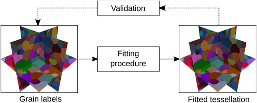
FIGURE 2. Schematic overview of the fitting of tessellations to simulated image data having smooth grain boundaries and validation of the resulting fits. Orthogonal 2D slices through 3D datasets are shown.

FIGURE 3

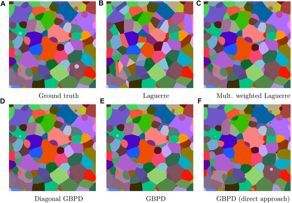
FIGURE 3. Two-dimensional slices through (A) the simulated ground truth image data and the corresponding fitted tessellations: (B)–(E) were obtained by the gradient descent-based method described in Section 2.3, whereas (F) followed from the direct approach described in Section 2.4.2.

TABLE 1

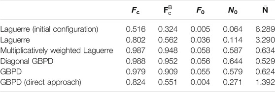
TABLE 1. Values of performance measures for various tessellation models fitted to the smooth simulated image data, considering the fraction of correctly assigned voxels F_c, the fraction of correctly assigned boundary voxels $F_{\mathrm{c}}^{\mathrm{B}}$, the fraction of empty cells F₀, the fraction of cells for which all cell neighbors are correct N₀, and the mean number of incorrect cell neighbors $\bar{N}$. The fits were obtained by the cross-entropy approach (“initial configuration”) described in Section 2.4.1, the gradient descent-based approach described in Section 2.3, and the “direct approach” described in Section 2.4.2.

3.2.2 Perturbed Grain Labels

One of the main goals of the present paper is to investigate the fitting of tessellations to image data containing rough grain boundaries—which may result, for example, from measurement uncertainties. For an in-depth analysis of this scenario, the grain labels of the simulated image data from Section 3.2.1 were perturbed such that the originally smooth boundaries exhibited a similar degree of roughness as in the experimental image data. With this approach, it was possible to vary the intensity of the perturbation and to study the robustness of the fitting even for degrees of boundary roughness well beyond that observed in experiment. Another benefit was the ability to evaluate the goodness of fit with respect to the (true) smooth grain boundaries instead of with respect to the perturbed grain boundaries that were input to the fitting procedure (Figure 4).

FIGURE 4

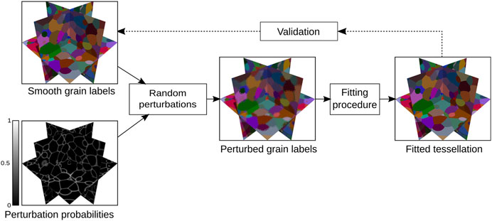
FIGURE 4. Schematic overview of the generation of perturbed simulated grain labels and validation of their fits. Orthogonal 2D slices through 3D datasets are shown.

Intuitively, the perturbed simulated image data was generated by computing a binary image of the grain boundaries from the smooth simulated image I_sim considered in Section 3.2.1. Then, the grain boundaries were blurred. The resulting grayscale image was used to define probabilities with which the grain labels of voxels in I_sim were reassigned to labels drawn from each voxel’s near vicinity. This way, a grain label is most likely to be changed when a voxel is located near a grain boundary, while the labels of voxels closer to a grain center will usually remain unchanged. A similar tendency is evident in the raw experimental data (Figure 1).

More precisely, the perturbation probabilities were obtained as follows. First, a ‘subvoxel’ boundary image $I_{\mathrm{b}}:{\mathcal{W}}_{\mathrm{p}\mathrm{e}\mathrm{r}\mathrm{t}}^{\ast }\to \{\mathrm{0,1}\}$ of the smooth simulated image I_sim was computed according to

$I_{\mathrm{b}}\left(y\right)=\left\{\begin{array}{cc}1\hfill & \text{if\hspace{0.17em}}\#{\mathcal{N}}^{\mathrm{b}}\left(y\right)>1,\hfill \\ 0\hfill & \text{otherwise,}\hfill \end{array}\right.$

with

${\mathcal{N}}^{\mathrm{b}}\left(y\right)=\left\{I_{\mathrm{s}\mathrm{i}\mathrm{m}}\left(x_1,x_2,x_3\right):x_k=\frac{y_k\pm 1}{2}\text{\hspace{0.17em}if\hspace{0.17em}}{y}_k\text{\hspace{0.17em}odd,\hspace{0.17em}and\hspace{0.17em}}{x}_k=\frac{y_k}{2}\text{\hspace{0.17em}if\hspace{0.17em}}{y}_k\text{\hspace{0.17em}even},k=\mathrm{1,2,3}\right\}$

for $y=(y_1,y_2,y_3)\in {\mathcal{W}}_{\mathrm{p}\mathrm{e}\mathrm{r}\mathrm{t}}^{\ast }={\{0,\dots ,598\}}^3$. This means I_b(y) is labeled as a boundary voxel whenever the set ${\mathcal{N}}^{\mathrm{b}}(y)$ contains at least two distinct grain labels. Effectively, this amounts to assigning boundary locations by considering an upsampled version of I_sim with nearly twice the number of voxels in each spatial dimension. So, if two neighboring voxels in I_sim have different labels, a boundary is drawn between these voxels in I_b—see Figure 5. Next, a Gaussian blur (Russ and Neal, 2017) with standard deviation σ ≥ 0 (where σ = 0 implies no blurring) was applied to the boundary image I_b to obtain the blurred boundary image $I_{\mathrm{b}\mathrm{l}\mathrm{u}\mathrm{r}}:{\mathcal{W}}_{\mathrm{p}\mathrm{e}\mathrm{r}\mathrm{t}}^{\ast }\to [\mathrm{0,1}]$. Here, the values of voxels in ${\mathcal{W}}_{\mathrm{p}\mathrm{e}\mathrm{r}\mathrm{t}}^{\ast }$ are scaled such that their minimum and maximum are equal to 0 and 1, respectively. Since σ determines how far into a grain the perturbations occur, we call it the perturbation spread. Finally, the perturbation probability image $I_{\mathrm{p}\mathrm{r}\mathrm{o}\mathrm{b}}:{\mathcal{W}}_{\mathrm{p}\mathrm{e}\mathrm{r}\mathrm{t}}\to [\mathrm{0,1}]$ was acquired by a subsequent downsampling to the original resolution of I_sim:

$I_{\mathrm{p}\mathrm{r}\mathrm{o}\mathrm{b}}\left(x\right)=\frac{1}{8}\sum _{z_1,z_2,z_3\in \left\{\mathrm{0,1}\right\}}{I}_{\mathrm{b}\mathrm{l}\mathrm{u}\mathrm{r}}\left(2x_1+z_1,2x_2+z_2,2x_3+z_3\right)$

for $x=(x_1,x_2,x_3)\in {\mathcal{W}}_{\mathrm{p}\mathrm{e}\mathrm{r}\mathrm{t}}={\mathcal{W}}_{\mathrm{s}\mathrm{i}\mathrm{m}}$. During this calculation, values outside the domain of I_blur were set equal to 0.

FIGURE 5

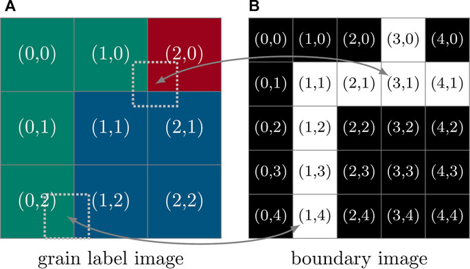
FIGURE 5. Two-dimensional example of (A) a 3 × 3-pixel grain label image I_sim with three grain labels (green, red and blue) and (B) its “subvoxel” boundary image I_b. Two pixels of the boundary image (one at location (3, 1) and another at (1, 4)) are superimposed on their corresponding locations in the grain label image (dotted squares). Effectively, the set ${\mathcal{N}}^{\mathrm{b}}(\cdot )$ contains all grain labels covered by these shifted pixels. The cardinality of the set ${\mathcal{N}}^{\mathrm{b}}((\mathrm{1,4}))$ is therefore 2, whereas $\#{\mathcal{N}}^{\mathrm{b}}((\mathrm{3,1}))=3$. If the indices specifying the location of a pixel in the boundary image are all even, this pixel lies entirely within the bounds of a single pixel in the grain label image; consequently, the cardinality of ${\mathcal{N}}^{\mathrm{b}}(\cdot )$ is always 1, and the pixel in I_b will always be assigned the value of zero (shaded black in the boundary image).

The smooth simulated image I_sim was perturbed by considering the random variables Z_x with values in {1, …, n_GT} such that

$Z_x=\left\{\begin{array}{cc}{I}_{\mathrm{s}\mathrm{i}\mathrm{m}}\left(x\right)\hfill & \text{with\hspace{0.17em}probability\hspace{0.17em}}{I}_{\mathrm{p}\mathrm{r}\mathrm{o}\mathrm{b}}\left(x\right),\hfill \\ I_{\mathrm{s}\mathrm{i}\mathrm{m}}\left(y\right)\hfill & \text{with\hspace{0.17em}probability\hspace{0.17em}}1-I_{\mathrm{p}\mathrm{r}\mathrm{o}\mathrm{b}}\left(x\right),\hfill \end{array}\right.$

for each voxel $x\in {\mathcal{W}}_{\mathrm{p}\mathrm{e}\mathrm{r}\mathrm{t}}$, where y is the closest voxel in I_sim to x for which I_sim(y) ≠ I_sim(x) (ties are broken by choosing a grain label uniformly at random). We assume that all Z_x are stochastically independent of each other. The perturbation $I_{\mathrm{p}\mathrm{e}\mathrm{r}\mathrm{t}}:{\mathcal{W}}_{\mathrm{p}\mathrm{e}\mathrm{r}\mathrm{t}}\to \{1,\dots ,n_{\mathrm{G}\mathrm{T}}\}$ of the smooth simulated image I_sim was then obtained as a realization of the random variables ${\{Z_x\}}_{x\in {\mathcal{W}}_{\mathrm{p}\mathrm{e}\mathrm{r}\mathrm{t}}}$. Note that I_pert is a function of the perturbation spread σ ≥ 0 and that, even for the case σ = 0, perturbations can still occur within a voxel of the grain boundaries, as I_prob can take non-zero values. Since there were no background voxels in I_pert, we set ${\mathcal{X}}^{\mathrm{F}}={\mathcal{W}}_{\mathrm{p}\mathrm{e}\mathrm{r}\mathrm{t}}$.

Several different values of the perturbation spread σ are considered in the present paper. In Figures 6, 2D slices through the resulting perturbed simulated image data are shown. For each of these datasets the same fittings as in the previous section were performed. As the perturbations are assumed to have originated from measurement errors, the fits were compared to the smooth image data instead of evaluating the goodness of fit with respect to the perturbed image data (cf. Figure 4). The dependence of the quality of fit on the perturbation spread σ is visualized in Figure 7. For σ = 1, a visual comparison of the fitted tessellations to the smooth simulated image data is shown in Figure 8, whereas in Table 2 numerical fitting results are given.

FIGURE 6

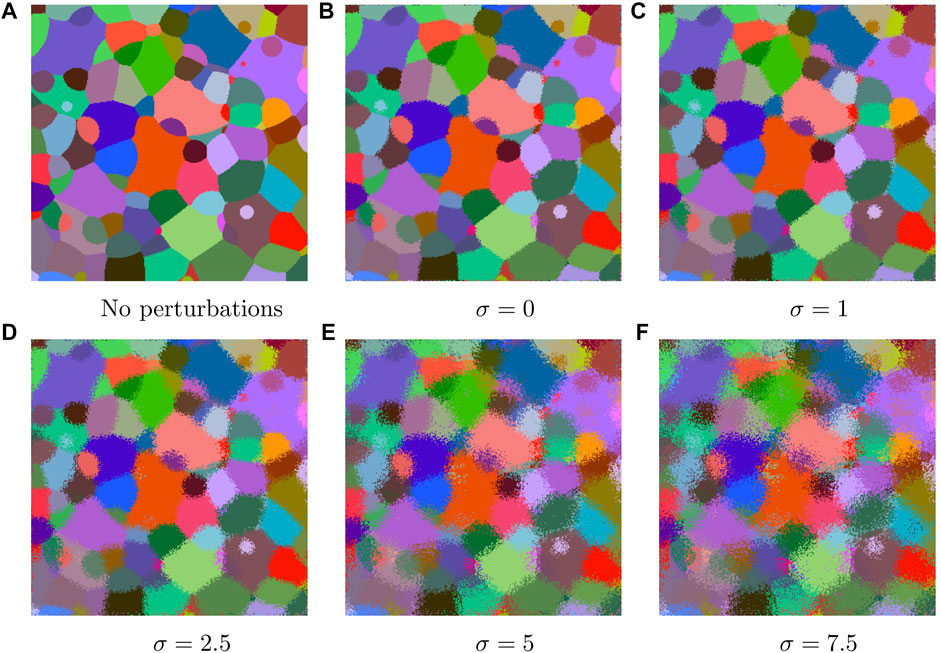
FIGURE 6. Two-dimensional slices through the simulated image data I_sim following perturbation of the latter with I_pert, shown in (A–F) for different values of the perturbation spread σ ≥ 0.

FIGURE 7

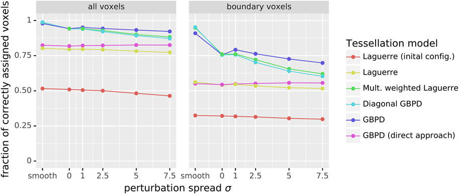
FIGURE 7. Fraction of correctly assigned voxels plotted against the perturbation spread σ, evaluated for all voxels in the image dataset and for the boundary voxels.

FIGURE 8

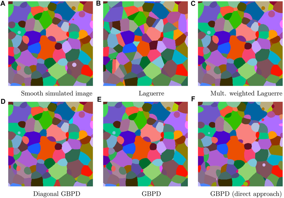
FIGURE 8. Two-dimensional slices through (A) the smooth simulated image I_sim and (B)–(F) tessellations fitted to the perturbed simulated image data I_pert with σ = 1. The fits in (B)–(E) were obtained by the gradient descent-based method described in Section 2.3, whereas (F) followed from the direct approach described in Section 2.4.2.

TABLE 2

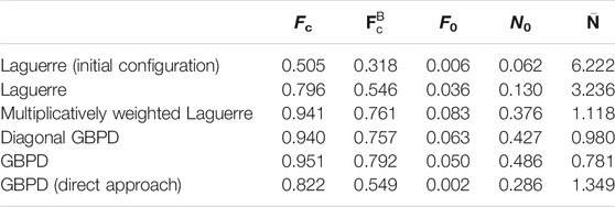
TABLE 2. Values of performance measures for various tessellation models fitted to the perturbed simulated image I_pert with σ = 1 and evaluated with respect to the smooth simulated image I_sim.

3.3 Experimental Data

In this section, the fitting method described in Section 2.3 is tested with realistic grain boundaries. For this purpose, experimental image data obtained from a 3DXRD mapping of an AlCu sample (Section 2.1) was used. As with the simulated data of Section 3.2, we first consider image data with smooth grain boundaries before tackling a dataset with rougher boundaries (Figure 1). The goal is to assess the robustness of the fitting procedure with respect to real-world grain boundary perturbations—originating, e.g., from measurement uncertainties—and also to determine whether the custom of preprocessing raw experimental image data to obtain smoother (and, thus, physically more sensible) grain boundaries prior to fitting is actually necessary.

3.3.1 Smoothed Grain Boundaries

The image I_E,smooth gained from an AlCu sample exhibits smooth grain boundaries after being preprocessed with a phase field algorithm (Section 2.1). Tessellation fitting was performed with respect to all foreground voxels ${\mathcal{X}}^{\mathrm{F}}=\{x\in {\mathcal{W}}_{\mathrm{E},\mathrm{s}\mathrm{m}\mathrm{o}\mathrm{o}\mathrm{t}\mathrm{h}}:I_{\mathrm{E},\mathrm{s}\mathrm{m}\mathrm{o}\mathrm{o}\mathrm{t}\mathrm{h}}(x)>0\}$. The numerical results of the fitting are presented in Table 3. Because 2D slices through these fitted tessellations were found to be qualitatively similar to those shown in Figure 9—which were obtained from fits to the raw experimental map—we omit the images of tessellations fitted to the smoothed experimental data.

TABLE 3

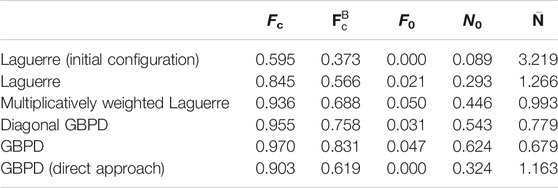
TABLE 3. Values of performance measures for various tessellation models fitted to the smoothed experimental image data.

FIGURE 9

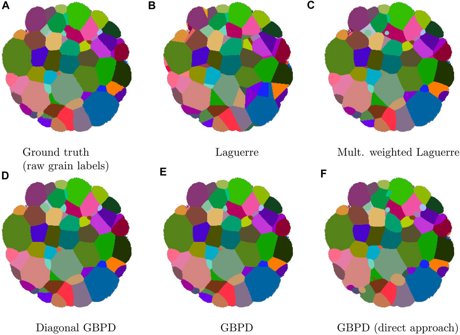
FIGURE 9. Two-dimensional slices through (A) the raw experimental ground truth image data and (B)–(F) the corresponding fitted tessellations. The fits in (B)–E) were obtained by the gradient descent-based method described in Section 2.3, whereas (F) followed from the direct approach described in Section 2.4.2. Note that the 2D slice shown in (A) differs from that shown in Figure 1A.

3.3.2 Raw Grain Boundaries

The raw experimental image data, described by the mapping I_E,raw (see Section 2.1), was not subjected to the phase field smoothing step following tomographic reconstruction of the 3DXRD measurement. For this reason, artifacts attributable to measurement uncertainties are visible at and near the grain boundaries (cf. Figure 1A). In contrast to the fitting of tessellations to the perturbed simulated image data of Section 3.2.2, in the present case we evaluate the quality of fit with respect to the same data that was used as the input dataset (i.e., the raw experimental map). One might consider treating I_E,smooth as a good approximation of the true, unobserved grain boundaries; however, since some grains were removed by the smoothing step, the number of grains in the ‘reference’ dataset would differ from the number of cells in the fitted tessellations. As a result, the performance measures of Section 3.1 would no longer be applicable. A visual comparison of the fits to the raw experimental image data is shown in Figure 9, and the numerical results are presented in Table 4. Here, all foreground voxels ${\mathcal{X}}^{\mathrm{F}}=\{x\in {\mathcal{W}}_{\mathrm{E},\mathrm{s}\mathrm{m}\mathrm{o}\mathrm{o}\mathrm{t}\mathrm{h}}:I_{\mathrm{E},\mathrm{s}\mathrm{m}\mathrm{o}\mathrm{o}\mathrm{t}\mathrm{h}}(x)>0\}$ were considered during the fitting.

TABLE 4

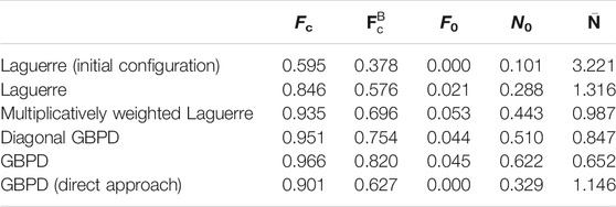
TABLE 4. Values of performance measures for various tessellation models fitted to the raw experimental image data.

4 Discussion

4.1 Fitting Results

As seen in Section 3.2.1, the fitted multiplicatively weighted Laguerre tessellation, the diagonal GBPD and the GBPD matched the smooth simulated image data very well, and a near perfect voxelwise accuracy was obtained. Between these tessellation models, there were only minor differences in the goodness of fit. Most notably, the GBPD was slightly worse at reconstructing the boundary voxels (see Table 1). Nevertheless, no significant decline in goodness of fit was observed even for the tessellation models that employ more parameters than necessary to describe the ground truth image data (which was generated from a multiplicatively weighted Laguerre tessellation). Furthermore, except for the number of empty cells, the gradient descent-based fitting procedure described in Section 2.3 achieved a notably better fit than the good results obtained by the direct approach of Teferra and Rowenhorst (2018) (see Section 2.4.2). On the other hand, in light of the results given in Table 1 for the initial Laguerre tessellation and the improved generators that resulted from the fitting procedure of Section 2.3, it is clear that the Laguerre tessellations with their flat boundaries (see Figure 3B) lacked sufficient flexibility for an accurate reconstruction of the ground truth data. However, the gradient descent-based fitting procedure still managed to bring about a significant improvement compared to the initial generators from the cross-entropy approach. This can likely be traced to the fact that the gradient descent-based approach considers a volume-based objective function (see Section 2.3) rather than an interface-based one (see Section 2.4.1). In general, we cannot expect to solve such a high-dimensional optimization problem by finding its global optimum; this would be equivalent to finding a perfect reconstruction of the multiplicatively weighted Laguerre tessellation that underlays the ground truth image data. Nevertheless, the fitted tessellations were quite close to the optimum, despite having been obtained by a local optimization method.

When it comes to the perturbed simulated image data investigated in Section 3.2.2, it is somewhat surprising how well the voxels of the smooth simulated image data could be reconstructed even from very noisy input image data (see Figure 7). As the same effect is observed for all three fitting methods considered in the present paper—i.e., the cross-entropy approach (Section 2.4.1), the direct approach (Section 2.4.2), and the gradient descent-based method (Section 2.3)—we attribute this robustness against perturbations to the inherent smoothing property of tessellations. Another observation that might surprise is the finding that the results for the direct approach were practically independent of the perturbation spread σ, but, just as in the case of the smooth simulated dataset, the gradient descent-based fitting procedure of Section 2.3 was able to surpass the direct method. The proposed method also achieved a better accuracy of the boundary voxels. In the latter case, however, some degradation could be observed with increasing σ. Some part of this degradation can be explained by the fact that a procedure producing more accurate approximations of the grain boundaries in the first place is going to be more sensitive to noise in the grain boundaries. Naturally, the deterioration in the fit of the boundary voxels also influences the considered grain neighborhood characteristics N₀ and $\bar{N}$—compare Tables 1, 2. Nevertheless, the decline in goodness of fit with σ is still well within reason, given the high noise level of the input image data (see Figure 6). In fact, from a visual comparison of the raw experimental image data in Figure 1B to the perturbed simulated image data in Figure 6, it can be seen that the case with the lowest level of noise (i.e., σ = 0) comes closest to the considered experimental data. This indicates that the gradient descent-based fitting procedure described in Section 2.3 is not only able to deal with the present level of measurement artifacts but also with much noisier scenarios.

For the experimental image data investigated in Sections 3.3.1, 3.3.2, quite high voxelwise accuracies F_c and $F_{\mathrm{c}}^{\mathrm{B}}$ were observed, particularly for the more sophisticated tessellation models, as they are better at describing non-convex grain morphologies. Despite this fact, with respect to F_c and $F_{\mathrm{c}}^{\mathrm{B}}$ the simpler Laguerre tessellation does a better job of fitting the experimental datasets than the simulated image—compare Tables 3, 4; Table 1. The same is true when considering the grain neighborhood characteristics N₀ and $\bar{N}$. As could already be anticipated from our analysis of the perturbed simulated image data, there was no significant difference in goodness of fit to the smoothed versus to the raw experimental datasets (for all performance measures). This leads us to conclude that there is no benefit to smoothing the grain boundaries in experimental image data prior to tessellation fitting.

One of the main advantages of the gradient descent-based fitting procedure described in Section 2.3 compared to other optimization approaches lies in its runtime performance. This comes from the reformulation of the objective function and the resulting ability to employ efficient gradient descent optimization algorithms. Another reason is the fact that the objective function and its gradient can both be computed on multiple CPU cores or even on GPUs. This opens up the possibility of reducing the (wall clock) time for the fitting procedure by employing hardware having a higher degree of parallelism (such as GPUs), which would not be so readily feasible for sequential fitting procedures. As runtime benchmarks are notorious for their dependence on a multitude of factors (in this case, for example, on the number of generators/grains, the number of voxels, the computer hardware, etc.), the runtimes quoted in Table 5 for the fitting of tessellations to the smoothed experimental image data should be taken with a grain of salt. In this particular case, the slower fitting of the GBPD model than the other tessellations can be attributed not only to the increased number of parameters but, more importantly, to the fact that a less efficient software implementation had to be used to compute the GBPD distance function. That being said, to achieve such a high goodness of fit for a dataset with 531 × 321 × 321 voxels and 938 grains, the runtimes are quite competitive, especially for the other tessellation models.

TABLE 5

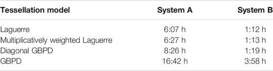
TABLE 5. Runtimes for the fitting of tessellation models to the smoothed experimental image dataset. System A employed only a CPU (Intel Core i7-4770K with four 3.50 GHz cores), whereas System B performed some of the computations on a GPU (CPU: AMD Ryzen 5 3600 with six 3.6 GHz cores; GPU: NVIDIA GeForce RTX 3060).

4.2 Other Fitting Approaches in the Literature

The fitting results for the direct approach of Teferra and Rowenhorst (2018) (Section 2.4.2) were discussed in the previous section. For all datasets, the direct approach delivered reasonably good fits of GBPDs, but they were consistently worse than those obtained by the gradient descent-based fitting procedure of Section 2.3. The only exception here is the fact that the direct method produced very few empty cells. Its main benefit, however, is the very short runtime of only a couple of seconds. Therefore, the direct approach is a good choice if a tessellation must be found quickly, but if the focus lies on the quality of fit, the gradient descent-based method developed in the present paper may be more suitable.

In Šedivý et al. (2016), still another method for fitting GBPDs was proposed, in which—similar to the present paper—a volume-based objective function is optimized. However, instead of a gradient descent method, Šedivý et al. employed a global stochastic optimization technique, the simulated annealing algorithm. As the name implies, this technique is inspired by the annealing (heat treatment) of metals. Specifically, during each iteration of the optimization, a random modification of the previous generators is proposed. These changes are accepted depending on whether the objective function is improved as well as on the current value of the ‘temperature.’ Here, the parameter ‘temperature’ governs the likelihood that a change in generators is accepted even though it leads to a worse value of the objective function. As the temperature is decreased over the course of the optimization, the probability increases that only improvements in the fit are accepted. In Šedivý et al. (2016), this fitting procedure was applied to both simulated and experimental image data. For the former case, which was a realization of a random GBPD, the quality of fit of the simulated annealing approach (F_c = 0.975, N₀ = 0.604, $\bar{N}=0.57$) was similar to the results obtained in Section 3.2.1 of the present paper. However, since the simulated datasets were drawn from two different models (GBPD vs. multiplicatively weighted Laguerre tessellation), direct comparison warrants caution. Regarding the runtime of the fitting routine, it is mentioned in Šedivý et al. (2016) that roughly 19 h were needed to carry out 10 million optimization iterations on an Intel Xeon E3-1240 CPU with four 3.4 GHz cores (slightly slower than the Intel Core i7-4770K used in the present paper). The procedure stopped after 13 million iterations, which corresponds to a total runtime of about 24 h. When comparing this to the 16:42 h that the same fitting took in the present paper (see Table 5), we note that the dataset considered by Šedivý et al. had only about a 10th the size (180³ vs. 531 × 321 × 321 voxels) but more than twice as many grains (1894 vs. 938 grains). A direct comparison to their experimental dataset is omitted, as the two datasets are quite different. In summary, the goodness of fit achieved by the simulated annealing approach applied to simulated data was similar to that achieved by the gradient descent-based fitting procedure of the present paper, but the runtime reported in Šedivý et al. (2016) was significantly longer.

5 Conclusion

In this paper, a novel method for fitting distance-based tessellations, such as the Laguerre tessellation or generalized balanced power diagrams, to 3D image data was developed. With this approach, it is possible to obtain parametric representations of the curved grain boundaries of real polycrystalline materials. The method employs efficient gradient descent optimization, with the technique proving to be capable of reconstructing a tessellation from its discretized image. Nearly identical fits were obtained when the procedure was applied to smoothed versus raw experimental data. From the observed robustness against noise in the input image data, we conclude that there is no benefit to smoothing an experimental image dataset prior to fitting it with a tessellation model.

The proposed method could facilitate the study of physical phenomena like curvature-driven grain growth, in which smooth representations of grain boundaries—such as those provided by tessellation models—are required for accurate calculations. Furthermore, the fitted tessellations could serve as the basis for stochastic models of polycrystalline microstructures. These models could potentially enable researchers to investigate mechanical properties of material samples in silico instead of through resource-intensive laboratory experimentation.

Data Availability Statement

The datasets presented in this article are not readily available because they are part of ongoing research. Requests to access the datasets should be directed to LP, lukas.petrich@uni-ulm.de.

Author Contributions

Tomographic image data of the AlCu specimen were provided by MW and CK. The basic idea of the gradient-based fitting approach came from OF. The software implementation and computer experiments were performed by LP. Main parts of the paper were written by LP and CK. All authors discussed the results and contributed to writing of the manuscript. CK and VS designed and supervised the research.

Funding

The authors gratefully acknowledge partial financial support provided by the Deutsche Forschungsgemeinschaft (DFG) through projects KR 1658/9-1 and SCHM 997/41-1. In addtion, The authors are grateful to the Japan Synchrotron Radiation Research Institute for the allotment of beamtime on beamline BL20XU of SPring-8 (Proposal 2015A1580).

Conflict of Interest

The authors declare that the research was conducted in the absence of any commercial or financial relationships that could be construed as a potential conflict of interest.

Publisher’s Note

All claims expressed in this article are solely those of the authors and do not necessarily represent those of their affiliated organizations, or those of the publisher, the editors and the reviewers. Any product that may be evaluated in this article, or claim that may be made by its manufacturer, is not guaranteed or endorsed by the publisher.

References

Abadi, M., Agarwal, A., Barham, P., Brevdo, E., Chen, Z., Citro, C., et al. (2015). TensorFlow: Large-Scale Machine Learning on Heterogeneous Systems. Software available from tensorflow.org.

Google Scholar

Allen, J. M., Weddle, P. J., Verma, A., Mallarapu, A., Usseglio-Viretta, F., Finegan, D. P., et al. (2021). Quantifying the Influence of Charge Rate and Cathode-Particle Architectures on Degradation of Li-Ion Cells through 3D Continuum-Level Damage Models. J. Power Sourc. 512, 230415. doi:10.1016/j.jpowsour.2021.230415

CrossRef Full Text | Google Scholar

Alpers, A., Brieden, A., Gritzmann, P., Lyckegaard, A., and Poulsen, H. F. (2015). Generalized Balanced Power Diagrams for 3D Representations of Polycrystals. Phil. Mag. 95, 1016–1028. doi:10.1080/14786435.2015.1015469

CrossRef Full Text | Google Scholar

Altendorf, H., Latourte, F., Jeulin, D., Faessel, M., and Saintoyant, L. (2014). 3D Reconstruction of a Multiscale Microstructure by Anisotropic Tessellation Models. Image Anal. Stereol 33, 121–130. doi:10.5566/ias.v33.p121-130

CrossRef Full Text | Google Scholar

Audet, C., and Hare, W. (2017). Derivative-Free and Blackbox Optimization. Springer.

Google Scholar

Aurenhammer, F., Klein, R., and Lee, D.-T. (2013). Voronoi Diagrams And Delaunay Triangulations. World Scientific.

Google Scholar

Bourne, D. P., Kok, P. J. J., Roper, S. M., and Spanjer, W. D. T. (2020). Laguerre Tessellations and Polycrystalline Microstructures: a Fast Algorithm for Generating Grains of Given Volumes. Phil. Mag. 100, 2677–2707. doi:10.1080/14786435.2020.1790053

CrossRef Full Text | Google Scholar

Burnett, T. L., Kelley, R., Winiarski, B., Contreras, L., Daly, M., Gholinia, A., et al. (2016). Large Volume Serial Section Tomography by Xe Plasma FIB Dual Beam Microscopy. Ultramicroscopy 161, 119–129. doi:10.1016/j.ultramic.2015.11.001

PubMed Abstract | CrossRef Full Text | Google Scholar

Chiu, S. N., Stoyan, D., Kendall, W. S., and Mecke, J. (2013). Stochastic Geometry and its Applications. 3 edn. J. Wiley & Sons.

Google Scholar

Dake, J. M., Oddershede, J., Sørensen, H. O., Werz, T., Shatto, J. C., Uesugi, K., et al. (2016). Direct Observation of Grain Rotations during Coarsening of a Semisolid Al-Cu alloy. Proc. Natl. Acad. Sci. USA 113, E5998–E6006. doi:10.1073/pnas.1602293113

PubMed Abstract | CrossRef Full Text | Google Scholar

Furat, O., Petrich, L., Finegan, D. P., Diercks, D., Usseglio-Viretta, F., Smith, K., et al. (2021). Artificial Generation of Representative Single Li-Ion Electrode Particle Architectures from Microscopy Data. Npj Comput. Mater. 7, 105. doi:10.1038/s41524-021-00567-9

CrossRef Full Text | Google Scholar

Goodfellow, I., Bengio, Y., and Courville, A. (2016). Deep Learning. MIT Press.

Google Scholar

Kingma, D. P., and Ba, J. (2015). “Adam: a Method for Stochastic Optimization,” in 3rd International Conference On Learning Representations, ICLR 2015. Editors Y. Bengio, and Y. LeCun.

Google Scholar

Krill III, C. E., and Chen, L.-Q. (2002). Computer Simulation of 3-D Grain Growth Using a Phase-Field Model. Acta Materialia 50, 3059–3075. doi:10.1016/s1359-6454(02)00084-8

CrossRef Full Text | Google Scholar

Lautensack, C., and Zuyev, S. (2008). Random Laguerre Tessellations. Adv. Appl. Probab. 40, 630–650. doi:10.1239/aap/1222868179

CrossRef Full Text | Google Scholar

Liebscher, A. (2015). Laguerre Approximation of Random Foams. Phil. Mag. 95, 2777–2792. doi:10.1080/14786435.2015.1078511

CrossRef Full Text | Google Scholar

Lyckegaard, A., Lauridsen, E. M., Ludwig, W., Fonda, R. W., and Poulsen, H. F. (2011). On the Use of Laguerre Tessellations for Representations of 3D Grain Structures. Adv. Eng. Mater. 13, 165–170. doi:10.1002/adem.201000258

CrossRef Full Text | Google Scholar

Møller, J. (1994). Lectures on Random Voronoi Tessellations. Springer.

Google Scholar

Okabe, A., Boots, B., Sugihara, K., and Chiu, S. N. (2000). Spatial Tessellations Concepts and Applications of Voronoi Diagrams. 2 edn. J. Wiley & Sons.

Google Scholar

Petrich, L., Staněk, J., Wang, M., Westhoff, D., Heller, L., Šittner, P., et al. (2019). Reconstruction of Grains in Polycrystalline Materials from Incomplete Data Using Laguerre Tessellations. Microsc. Microanal 25, 743–752. doi:10.1017/s1431927619000485

PubMed Abstract | CrossRef Full Text | Google Scholar

Poulsen, H. F. (2004). Three-Dimensional X-Ray Diffraction Microscopy: Mapping Polycrystals and Their Dynamics. Springer.

Google Scholar

Quey, R., and Renversade, L. (2018). Optimal Polyhedral Description of 3D Polycrystals: Method and Application to Statistical and Synchrotron X-ray Diffraction Data. Comp. Methods Appl. Mech. Eng. 330, 308–333. doi:10.1016/j.cma.2017.10.029

CrossRef Full Text | Google Scholar

Raabe, D. (1998). Computational Materials Science. Wiley VCH.

Google Scholar

Rubinstein, R. Y., and Kroese, D. P. (2004). The Cross-Entropy Method. Springer.

Google Scholar

Russ, J. C., and Neal, F. B. (2017). The Image Processing Handbook. 7 edn. Boca Raton: CRC Press.

Google Scholar

Schmidt, S. (2014). GrainSpotter: a Fast and Robust Polycrystalline Indexing Algorithm. J. Appl. Cryst. 47, 276–284. doi:10.1107/s1600576713030185

CrossRef Full Text | Google Scholar

Schmidt, S. (2005). GrainSweeper. Available at: https://svn.code.sf.net/p/fable/code/GrainSweeper. [Accessed August 17, 2021].

Google Scholar

Schwartz, A., Kumar, M., Adams, B., and Field, D. (2009). Electron Backscatter Diffraction in Materials Science. Springer.

Google Scholar

Šedivý, O., Brereton, T., Westhoff, D., Polívka, L., Beneš, V., Schmidt, V., et al. (2016). 3D Reconstruction of Grains in Polycrystalline Materials Using a Tessellation Model with Curved Grain Boundaries. Phil. Mag. 96, 1926–1949.

Google Scholar

Šedivý, O., Westhoff, D., Kopeček, J., Krill, C. E., and Schmidt, V. (2018). Data-driven Selection of Tessellation Models Describing Polycrystalline Microstructures. J. Stat. Phys. 172, 1223–1246.

Google Scholar

Spettl, A., Brereton, T., Duan, Q., Werz, T., Krill, C. E., Kroese, D. P., et al. (2016). Fitting Laguerre Tessellation Approximations to Tomographic Image Data. Phil. Mag. 96, 166–189. doi:10.1080/14786435.2015.1125540

CrossRef Full Text | Google Scholar

Teferra, K., and Graham-Brady, L. (2015). Tessellation Growth Models for Polycrystalline Microstructures. Comput. Mater. Sci. 102, 57–67. doi:10.1016/j.commatsci.2015.02.006

CrossRef Full Text | Google Scholar

Teferra, K., and Rowenhorst, D. J. (2018). Direct Parameter Estimation for Generalised Balanced Power Diagrams. Phil. Mag. Lett. 98, 79–87. doi:10.1080/09500839.2018.1472399

CrossRef Full Text | Google Scholar

Wang, K. G., and Glicksman, M. (2007). “Ostwald Ripening in Materials Processing,” in Materials Processing Handbook. Editors J. R. Groza, J. F. Shackelford, E. J. Lavernia, and M. T. Powers (Boca Raton: CRC Press), 75–94. doi:10.1201/9781420004823.ch5

CrossRef Full Text | Google Scholar

Westhoff, D., Skibinski, J., Šedivý, O., Wysocki, B., Wejrzanowski, T., and Schmidt, V. (2018). Investigation of the Relationship between Morphology and Permeability for Open-Cell Foams Using Virtual Materials Testing. Mater. Des. 147, 1–10. doi:10.1016/j.matdes.2018.03.022

CrossRef Full Text | Google Scholar

Zaefferer, S., Wright, S. I., and Raabe, D. (2008). Three-dimensional Orientation Microscopy in a Focused Ion Beam-Scanning Electron Microscope: a New Dimension of Microstructure Characterization. Metall. Mater. Trans. A. 39, 374–389. doi:10.1007/s11661-007-9418-9

CrossRef Full Text | Google Scholar