- School of Civil Engineering, Southeast University, Nanjing, China
The identification of fatigue crack initiation sites (FCISs) is routinely performed in the field of engineering failure analyses; this process is not only time-consuming but also knowledge-intensive. The emergence of convolutional neural networks (CNNs) has inspired numerous innovative solutions for image analysis problems in interdisciplinary fields. As an explorative study, we trained models based on the principle of transfer learning using three state-of-the-art CNNs, namely VGG-16, ResNet-101, and feature pyramid network (FPN), as feature extractors, and a faster R-CNN as the backbone to establish models for FCISs detection. The models showed application-level detection performance, with the highest precision reaching up to 95.9% at a confidence threshold of 0.6. Among the three models, the ResNet model exhibited the highest accuracy and lowest training cost. The performance of the FPN model closely followed that of the ResNet model with an advantage in terms of the recall.
Introduction
Fatigue fracture often occurs in engineering structures, such as aircrafts (Cowles, 1996), bridge (Guo et al., 2020), surgical implants (Huang et al., 2005), at variety scales. Fractographic studies via different types of microscopy techniques are key to identifying the causes and crack growth behaviors in fatigue-fractured components (Kushvaha and Tippur, 2014). However, fractographic analyses are not only time-consuming but also knowledge-intensive. Even an experienced material scientist may require a considerable amount of time in identifying the characteristics of new materials. Hence, it would be beneficial to develop methods that can accurately interpret most of the information in images without much human effort.
Convolutional neural networks (CNNs), which are inspired by the structure of actual visual systems, are one of the major advancements in the field of computer vision (Hubel and Wiesel, 1962; Fukushima, 1980; Lecun et al., 1998). With the popularity of deep CNNs in computer vision, they have been increasingly applied to the material science field, such as for predicting compounds (Xie and Grossman, 2018) and material properties (Sharma et al., 2020; Sharma and Kushvaha, 2020), analyzing X-ray diffraction patterns (Park et al., 2017), and classifying crystal structures (Ryan et al., 2018; Ziletti et al., 2018). In the years to come, it is reasonable to believe that CNNs will significantly accelerate the development of data-driven material science.
In a previous study (Wang et al., 2020), we employed machine learning approaches to recognize fatigue crack initiation sites (FCISs) in fractographic images of metallic compounds. The models were planned to be developed as an automatic FCIS detection module, which can be embedded with the observation systems attached to microscopes for a quick and accurate detection of FCISs. Given the lack of data, we selected a deep learning framework, namely the deeply supervised object detector (DSOD) (Shen et al., 2017), a framework that can train models of good performance from scratch. Although the DSOD has shown comparable or even superior accuracy in detecting objects in many domains compared with other state-of-the-art detectors (Shen et al., 2017), our results were below expectations. We explain some of the possible reasons for the difficulties in extracting features from FCISs as: 1) FCISs do not have clear boundaries for identification as in the case of objects in other detection tasks (e.g., animal, cars, or plants); 2) their features are typically blurry and nonobjective because of the low contrast and poor resolution, especially at low magnifications; 3) there is no distinction between foreground and background in most cases (as seen in Figure 1).
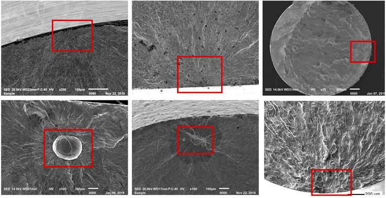
FIGURE 1. Examples of fatigue crack initiation sites (FCISs) of different types, morphologies, and locations. The red boxes indicate the FCISs.
Owing to the rapid development in computer vision algorithms, the above problem can be solved by transfer learning. Transfer learning is a machine learning method where the knowledge of an already trained model is reused as the starting point of a different but related problem (Pan and Yang, 2009; Weiss et al., 2016). In some problems where there is limited supply of training data, transfer learning can be utilized to develop efficient models. The transfer learning method has been successfully employed in many different areas, such as text mining (Pan et al., 2012), image classification (Quattoni et al., 2008; Zhu et al., 2011), spam filtering (Meng et al., 2010), and speech emotion recognition (Coutinho et al., 2014; Song et al., 2014). There are many ways of transferring knowledge from one task to another. Using pre-trained networks is a highly effective transfer learning approach that can improve the detection capacity of a new model when data are insufficient. State-of-the-art deep architectures, such as VGG (named after the Visual Geometry Group at University of Oxford) (Simonyan and Zisserman, 2014), Residual Neural Network (ResNet) (He et al., 2016), and Inception (Szegedy et al., 2016), exhibit a good performance for classification and localization problems. Most object detection and segmentation architectures, such as the faster R-CNN (Ren et al., 2015), can be built based on previous models through the concept of transfer learning.
The region-based CNN (R-CNNs) family, namely the R-CNN, fast R-CNN, and faster R-CNN, was developed by Girshick and Ren (Girshick et al., 2014; Girshick, 2015; Ren et al., 2015) for object localization and recognition. The R-CNN algorithm is faster and more accurate than conventional object detectors (e.g., Histogram of Oriented Gradient, HOG), as the sliding windows are replaced by “selective search” to extract CNN features from each candidate region. However, the training phase is computationally slow because of the multi-stage pipeline training process (Girshick, 2015). In the fast R-CNN, the training process is accelerated by employing three different models instead of a single model to extract features and by exploiting a region of interest (RoI) pooling layer to share the computation. The faster R-CNN (Ren et al., 2015) was developed from the fast R-CNN, exhibiting improved training and detection speeds. The architecture comprises a region proposal network (RPN) and fast R-CNN network with shared convolutional (conv.) feature layers in a single unified model design.
The fast R-CNN and faster R-CNN are both initialized by taking the output of a pre-trained deep CNN, such as VGG-16, on large-scale datasets (Girshick, 2015; Ren et al., 2015). The fine-tuning conv. layers in the pre-trained VGG-16 model improved the mAP (mean average precision) of both algorithms (Girshick, 2015; Ren et al., 2015). Similarly, Oquab et al. (2014) transferred mid-level image features from a source task, for which a CNN was trained on the ImageNet (Deng et al., 2009) with a large number of labeled images, to target tasks by immigrating the pre-trained conv. layers (C1-C5). The results showed that the features transferred from the pre-trained CNNs could significantly improve the classification performance of the target task with limited training data. Through a survey, Weiss et al. (2016) reported that this type of fine-tuning process can be classified under feature-based transfer learning.
Apart from the VGG-based faster R-CNN and ZF net-based faster R-CNN, He et al. tested the performance of a ResNet-based faster R-CNN (He et al., 2016). As VGG-16 was replaced by ResNet-101, the faster R-CNN system improved the mAP (@[0.5,95]) by 6.0% on the COCO validation set (He et al., 2016). Lin et al. (2017) further updated the ResNet-based faster R-CNN by modifying the backbone with a feature pyramid network (FPN), achieving even better results on the COCO minimal set over several strong baselines. Shared features were found to be beneficial for marginally improved accuracy and reduced testing time.
Focusing on the detection of FCISs, we constructed three transfer learning models using the faster R-CNN as the backbone and three CNN architectures, namely VGG-16, ResNet-101, and FPN, as feature extractors. The datasets were composed of fractographic images containing various types of FCISs of metallic compounds. This interdisciplinary study aimed to propose effective transfer learning methods that can accurately detect FCISs with a limited amount of data. The purpose of this study was to explore the possibilities of employing machine learning approaches in identifying nonobjective features seen in material science images and inspire researchers to solve similar image-driven material problems.
The rest of this article is organized as follows: Extended Introduction of Related Work reviews the definition of transfer learning and its correlations with the computer vision approaches exploited in this study. Subsequently, a brief introduction to the development of faster R-CNN and relevant deep architectures (VGG-16, ResNet-101, and FPN) is given to help researchers from areas other than computer science, such as material scientists, to understand the salient features of the faster R-CNN-based object detectors. Experimental Works introduces the databases and training implementations of the three models in detail. In Results and Discussion, the performances of the models for FCIS detection are evaluated in terms of the detection accuracy, training ability, calculation efficiency, and calculation cost. Conclusion presents the conclusions drawn from the study results.
Extended Introduction of Related Work
Since this is an interdisciplinary study, we reviewed related concepts to help researchers from a non-computer-science background to understand the approaches used.
Transfer Learning
Transfer learning in general refers to machine learning approaches where knowledge gained in one task is reused to improve the learning of a related task. The reasons for using transfer learning are based on the fact that the successful application of a deep neural network depends on a tremendous amount of training or pre-training data. Such data are sometimes expensive or difficult to obtain, such as in the case of FCISs. Many examples have shown that transfer learning can be beneficial for problems where training and testing data are in different feature spaces or data distributions (Weiss et al., 2016). Transfer learning can be broadly categorized into inductive transfer learning, unsupervised transfer learning, and transductive transfer learning. Each category contains various sub-approaches (Pan and Yang, 2009; Weiss et al., 2016). The approaches most closely related to our work in computer vision are transfer learning methods with a pre-trained model/ConvNet (Convolutional Network) (Oquab et al., 2014; Schwarz et al., 2015). A pre-trained model is typically trained on large benchmark image datasets, such as the ImageNet, which contains rich feature representations from a low level to a high level (Zeiler and Fergus, 2014). These feature representations can be partly or entirely reused in other tasks simply by integrating the activated conv. layers in a new deep neural network as a feature extractor and then fine-tuning the layers of the pre-trained model via continuous backpropagation. Many applications (Oquab et al., 2014; Schwarz et al., 2015; Huh et al., 2016; Qian et al., 2016; Lucena et al., 2017) have shown that state-of-the-art object detectors can be built via this approach.
Faster R-CNN-Based Object Detectors
Faster R-CNN Baseline
As previously highlighted, the faster R-CNN was developed along the lines of R-CNN, fast R-CNN, and its previous versions (Du, 2018; Khan et al., 2019). The R-CNN marks one of the most important milestones in object detection. It is the first neural network that uses an object proposal algorithm called “selective search” to extract a manageable number of independent regions for classification and bounding-box regression. However, training an R-CNN model is expensive and slow because of the multiple steps involved in the process (Girshick et al., 2014). In contrast to using the R-CNN to extract CNN feature vectors independently for each region proposal, the fast R-CNN passes the entire image to the deeper VGG-16 network to generate a conv. feature map for sharing the computation among the region proposals (Girshick, 2015). For each object proposal, an RoI pooling layer is used to replace the last max-pooling layer in the pre-trained CNN for extracting a fixed-length feature vector. The fast R-CNN has two heads, namely a classification head and a bounding-box regression head, which are jointly trained using a multi-task loss L (Softmax Loss + SmoothL1 Loss) on each labeled RoI. Thus, the precision of the algorithm is improved. All the above steps are executed simultaneously, making this method faster than the R-CNN (Girshick, 2015).
Although the selective search approach in the R-CNN and fast R-CNN is a more efficient method for localizing objects than using the sliding window in CNN methods, the process is slow because of the large number of separate regional proposals (Du, 2018). The faster R-CNN replaces the selective search with an RPN to obtain an object proposal by sliding it on the last shared conv. layer of the pre-trained CNNs (VGG-16 or ZF-net) (Ren et al., 2015). To solve the shape variations of the objects in the RPN, anchor boxes are introduced in the faster R-CNN. At each sliding position, there are nine candidate anchors (3 scales × 3 aspect ratios), the probabilities of which being foreground (positive sample) or background (negative sample) are predicted by the RPN. For a positive sample, the intersection-over-union (IoU) ratio is greater than 0.7, whereas the IoU ratio of a negative sample is less than 0.3. For each region proposal, the RPN uses two fully connected (FC) layers to judge and select anchors according to the above rules. Thus, the RPN generates bounding boxes of various sizes and their probabilities of each class. The first-round proposal generated by the RPN is used to train the fast R-CNN and then initialize the RPN training process. Such an alternating process of training the fast R-CNN and then fine-tuning the RPN-specific layers is repeated until the result converges well (Ren et al., 2015).
Although the correlation between sharing features from pre-trained CNN layers and transfer learning is less emphasized for the fast R-CNN (Girshick, 2015), this point is highlighted in the case of the faster R-CNN as it has the advantage of sharing computation from the pre-trained conv. layers (Ren et al., 2015). As mentioned above, there is consensus that training an object detector on a small dataset using the already learned features from a CNN trained on large datasets can be categorized under transfer learning (Oquab et al., 2014; Akcay et al., 2016; Weiss et al., 2016; Khan et al., 2019). Based on the features of four different transfer learning approaches specified by Pan and Yang (2009), and examples given by Weiss et al. (2016), it can be deduced that using a pre-trained model for feature extraction represents a feature-based transfer learning approach.
ResNet-Based and FPN-Based Faster R-CNN
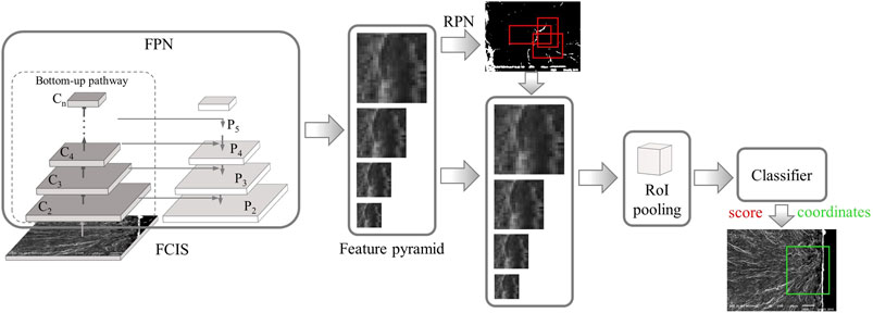
The integration of ResNet in the faster R-CNN was first proposed as an implementation of ResNet (He et al., 2016). He et al. (2016) employed the faster R-CNN as the baseline and replaced VGG-16 with ResNet-101 (101-layer residual net); the modified detector showed remarkable improvement in terms of the mAP, which was 6.9% [@.5] and 6.0% [@.5.95] higher than those of the original version on the COCO validation set. Lin et al. (2017) further modified the ResNet-based faster R-CNN with an FPN architecture. Instead of sharing the features of the last conv. layer in the pre-trained models, the FPN generates a feature pyramid from the ResNet backbone and multi-scale feature proposals in the RPN. Thus, the high-resolution features from the lower convolution layers and high-level semantic features could be used for prediction, thus improving the detection accuracy. The architecture details of the ResNet and FPN are introduced in the next section.
VGG, ResNet, and FPN
VGG
The VGG networks, introduced by Simonyan and Zisserman (2014), are known for their simplicity, homogenous topology, and relatively good network depth. In the ImageNet Large-Scale Visual Recognition Challenge (ILSVRC) held in 2013, it was found that small filters can improve the performance of CNNs (Zeiler and Fergus, 2014); therefore, only 3 × 3 conv. filters were used in all the layers of the VGG to increase the network depth. VGG-16 contains a total of 16 layers, including 13 conv. and three FC layers. The 13 conv. layers are segregated into five conv. blocks (2–3 conv. layer + ReLU) by max pooling. Max pooling layers are applied to obtain features at the end of each block. VGG networks show good performance in image classification (Simonyan and Zisserman, 2014). However, the training process is slow because of the large number of parameters [138 million parameters (Simonyan and Zisserman, 2014)].
ResNet
In conventional sequential architectures, the networks are constructed by stacking a set of “building blocks.” Therefore, they have drawbacks, such as gradient vanishing and network degradation, as the networks get deeper. The ResNet architecture proposed by He et al. (2016) exhibits an excellent performance in constructing deep networks without the above problems, using batch normalization and residual learning framework. Besides the common features in a CNN, such as convolution, pooling, activation, and FC layers, residual blocks are created in the residual learning framework by adopting identity/shortcut connections between every few stacked layers. A residual block is defined as in Eq. 1.
where x and H(x) are respectively the input and output vectors of a residual block whose dimensions are assumed to be identical. Therefore, the residual function
FPN
Low-level features extracted from lower layers, such as edges, curves, and dots, have high resolution and localization ability, but are less semantic. By contrast, the features generated at higher layers have high semantic value but have low resolution and localization accuracy (Zeiler and Fergus, 2014). With the introduction of a pyramid architecture composed of a bottom–up pathway, top–down pathway, and lateral connection, the FPN can combine low-resolution, semantically strong features with high-resolution, semantically weak features. In the original version of the FPN proposed by Lin et al. (2017), the ResNet is used as the backbone in the bottom–up pathway, and the features are extracted from the last layer in each residual block (denoted by C1, C2, …, C5). A 1 × 1 convolution filter is applied to the last feature map layer of the bottom–up pathway to reduce the dimension and is used as the starting layer (denoted by P5) of the top–down pathway. The top–down pathway creates new layers (P2, P3, and P4) by upsampling the previous layers with a factor of two using the nearest neighbors. A lateral connection is used at each pyramid level to merge the feature maps of the same spatial size (d = 256) from the bottom–up pathway and top–down pathway by element-wise addition. Since the FPN is not an object detector in itself, it should be integrated with other object detectors, e.g., the faster R-CNN. Unlike the VGG and ResNet in the faster R-CNN, which only transfer a single-scale feature map to create RoIs, the FPN generates a pyramid of feature maps. Thus, the RoIs are assigned to each pyramid level (Pk) of different scales (
Experimental Works
Datasets
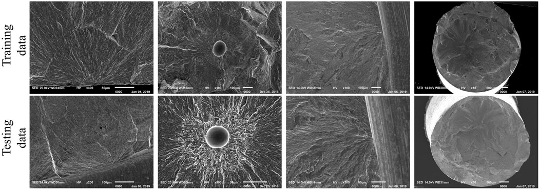
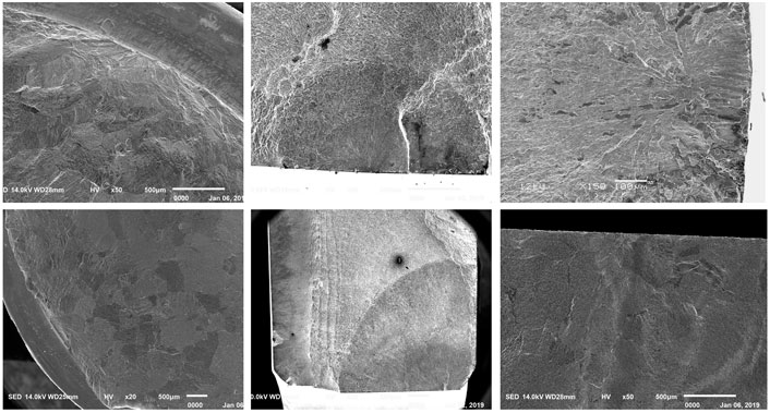
As a comparatively new machine learning domain, there is no “off-the-shelf” library for FCIS images. Therefore, we acquired data from the Internet by meticulous selection and from our in-house research works related to fatigue in metallic materials. The images were normalized for their format and size based on the standards used in the faster R-CNN (Ren et al., 2015). The datasets in the target task contain 291 images in total, with various FCIS details (such as location, morphology, size, and type) and image magnifications (×18∼×600) to ensure the generalization of the datasets. Following an existing data portioning ratio of 65% (training data):35% (testing data), the data were split into a training set (212 images) and a testing set (79 images). Instead of arbitrary selection, most of the testing data were chosen to maintain consistency in the distributions of the training and testing datasets (examples are shown in Figure 2). Several images of unusual FCIS types (Figure 3) were also added to the testing dataset to evaluate the generalization ability of the models. Although the unusual FCISs did contain some features of common FCISs, they also contained some patterns that were rare or absent in the training dataset. It should be emphasized that all the images in the training and testing datasets contained at least one FCIS.
The training data were annotated using LabelImg by a professional in the fatigue research field. LabelImg is an image annotation tool written in Python that can generate object bounding boxes. The Annotations were saved as XML files in the PASCAL VOC format.
Training on VGG-16 and ResNet-101-Based Faster R-CNN
The two deep neural networks (VGG-16 and ResNet-101) were pre-trained on the ImageNet dataset following the procedure provided in previous studies (Simonyan and Zisserman, 2014; He et al., 2016), thus attaining a robust hierarchy of features. For the pre-training, we implemented VGG-16 and ResNet-101 in the Caffe formats as done by Simonyan and Zisserman (2014) and Kaiming et al. (2015), respectively. Table 1 lists the details of the pre-training on VGG-16 and ResNet-101.
We used the frozen conv. layers of the pre-trained VGG-16/ResNet-101 (the weights were unchanged during model training) as feature extractors to train the RPN and detection network in the faster R-CNN (as shown in Figure 4). The training was carried out using the open-source faster R-CNN framework shared by Yang. (2017). The input images were resized and then cropped to dimensions of 224 × 224 following the method reported in (Simonyan and Zisserman, 2014; Ren et al., 2015; He et al., 2016). Each mini-batch contained only two images, thus avoiding overfitting on small datasets (Talo et al., 2019). All the training processes were terminated in 5,000 epochs, and the checkpoint was saved every 500 epochs. The initial learning rate was set to 0.01, and the rest of the optimization parameters were set as the default values in the torch. optim.SGD() function in Pytorch library; the weight decay and dampening were set to 0, and Nesterov was not applied. The experiments were performed on a single GeForce GTX 1060 GPU with 6 GB of memory.
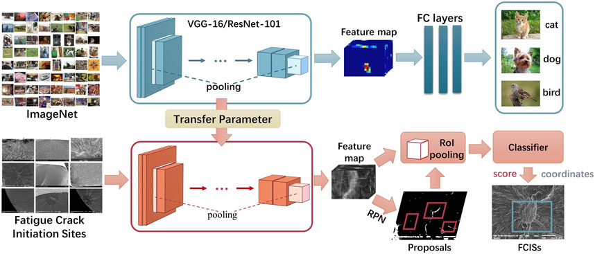
FIGURE 4. Schematic of fine-tuning the faster R-CNN with pre-trained parameters transferred from VGG-16 and ResNet-101.
Training on FPN-Based Faster R-CNN
As shown in Figure 5, the architecture of the FPN-based faster R-CNN was modified from that of the ResNet-based version. Hence, we only pre-trained the ResNet-101 baseline. The model was trained using the open-source Pytorch code, which was shared by Yang (2018). For comparison, we kept the training parameters consistent with the above experiments on VGG-16 and ResNet-101 based on the faster R-CNN. The model was trained for 5,000 epochs using stochastic gradient descent (SGD) iterative method, with an initial learning rate of 0.001 and a mini-batch size of 2.
Evaluation of Results
Typically, the IoU is often used for judging whether the predicted bounding box makes a good detection of the objects. The IoU is the ratio of the intersection area of the prediction bounding box and the ground truth box to their union area. However, it is difficult to use the IoU as an index for evaluating the results in this study because of the following two reasons: 1) The ground-truth bounding boxes were drawn based on manual estimation, which brings a high degree of arbitrariness; 2) It is difficult to set standards for drawing standardized ground-truth bounding boxes, because FCISs are varied in terms of the shape and size, and have no exact boundaries. Hence, the results were judged by the same material scientist who drew the ground-truth bounding boxes for a consistent judgment. We classified the prediction bounding boxes into three types in adherence to strict standards: true positive (TP), false positive (FP), and false negative (FN). The following are the definitions of the three types of results:
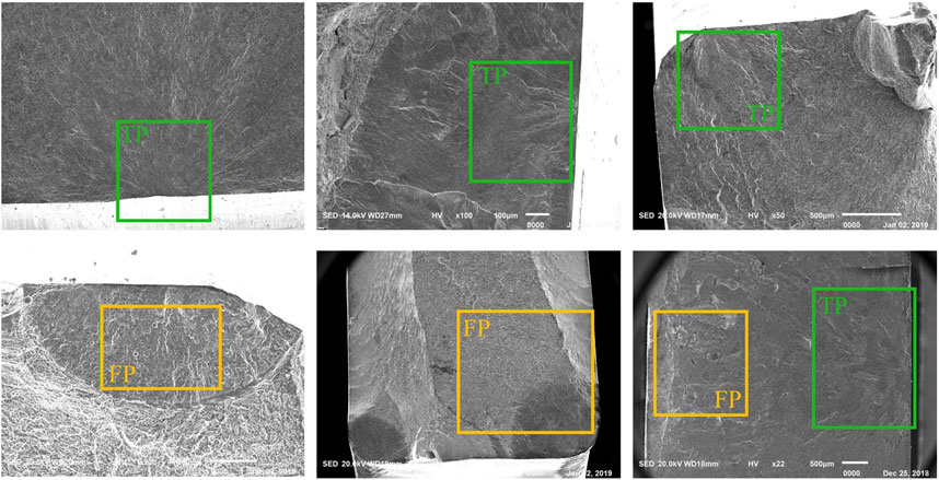
TP Results: The prediction boxes can accurately detect the FCISs or miss a marginally small part of FCISs but still cover most areas of the FCISs (as shown in Figure 6).
FP Results: The prediction boxes are at an incorrect part in the image or further away from the vicinity of fatigue crack initiation areas (as shown in Figure 6).
FN Results: No FCISs are detected in the images.
The statistical numbers of TP, FP, and FN are used for calculating the accuracy (A), precision (P), recall (R), and F1 score.
The accuracy represents the number of prediction boxes that are correct among the sample numbers. It is a quick index to determine the general performance of models.
The precision is the proportion of correct positive identifications among all the prediction boxes.
Recall is the proportion of correct positive predictions made from all the FCISs in the testing dataset. It can be considered as the sensitivity of the models in detecting FCISs, i.e., a higher R value indicates a stronger ability to detect FCISs under all conditions.
The F1 score is the harmonic mean of the combined precision and recall. A good F1 score (approaching 1) means that the model is less affected by false results.
All the above evaluation metrics vary with the changes in the confidence threshold set. The confidence threshold is the lower boundary of the confidence score of an object bounding box below which the results are removed. To obtain high recall values, which means that the TP predictions should be as accurate as possible, a low confidence threshold of 0.1 should be set to ensure that we would not miss any TP results that have low confidence values. A high threshold of 0.6 was used for comparison.
Results and Discussion
Model Accuracy
Table 2 gives a comparison of the performances of the three models at thresholds of 0.1 and 0.6. The three models are namely the VGG, ResNet, and FPN models. Remarkable improvements in the detection performance can be seen compared with our previous study on training a similar model from scratch using the DSOD algorithm (Wang et al., 2020). In the previous study, our best result was 22.1% in accurately detecting FCISs with just one bounding box and 24.0% for no valid results (i.e., FN results). Comparatively, even the VGG model, which exhibited a lower performance, could achieve ratios of 81.0 and 84.8% in accurately detecting FCISs with one bounding box at thresholds of 0.1 and 0.6, respectively.
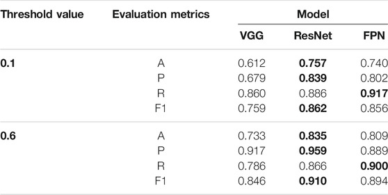
TABLE 2. Summary of elevation metrics of three different models at thresholds of 0.1 and 0.6 (The highest values are boldfaced).
At both the thresholds, we see that the ResNet model presents the best performance in terms of both the accuracy (0.839 and 0.959) and precision (0.757 and 0.835). The accuracy of the models is very close to the advanced studies on the applications of using artificial intelligence to solve material problems (Hemath et al., 2020; Kushvaha et al., 2020). Since there are no true negative results, higher accuracy values mean that the ResNet model has a lower portion of false results (FP and FN) among the observations, and higher precision values hint that the portions of FP were lower for the ResNet model.
The FPN model is slightly superior in terms of the recall (0.917 and 0.900) among the three methods, indicating that it can detect more accurate FCISs from existing FCISs in the testing dataset. The F1 score helps evaluate which model has a better overall performance in terms of both the precision and recall. Although the ResNet model achieves the highest F1 scores (0.862 and 0.910), which are just marginally higher than those of the FPN model (by 0.006) at both threshold values, the overall performances of the ResNet and FPN models are nearly identical.
The superiorities of the two models in terms of the precision and recall can help determine their application scenarios. If applications require a model that can recognize more FCISs in the images, the FPN model with higher recall values will be preferable; if the applications require highly certain results, the priority selection is the ResNet model. The VGG model is less competitive as all the evaluation metrics were the lowest.
The variations in the metrics between thresholds of 0.1 and 0.6 are compared in Figure 7. As the threshold increased from 0.1 to 0.6, the evaluation metrics of the three models improved except for the recall. The VGG model shows more distinct improvements in terms of the accuracy, precision, and F1 score, but a more significant drop in the recall value compared to the other two models. There is always a tradeoff between the precision and recall as the confidence threshold varies. Thus, the threshold values should be chosen depending on the application requirement.
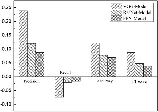
FIGURE 7. Changes in the accuracy, precision, recall, and F1 score of the three models for thresholds ranging from 0.1 to 0.6.
None of the three models are excellent for all types of FCISs, i.e., they perform well at detecting some FCISs but not so at detecting others; examples are given in Figure 8. Hence, it would be helpful to try different models when no TP results can be obtained using the employed model. Comparing Figure 3 with Figure 8, we find that some of the unusual FCISs (Figures 8B,C) can still be correctly detected by at least one of the three models, indicating that the models can detect features that are rare but relevant in the training dataset.
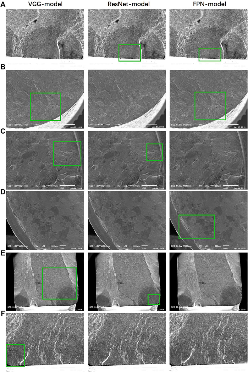
FIGURE 8. Examples of undetected cases: (A) only undetected by the VGG model; (B) only undetected by the ResNet model; (C) only undetected by the FPN model; (D) only correctly detected by the FPN model; (E) only correctly detected by the ResNet model; and (F) only correctly detected by the VGG model.
Training Loss
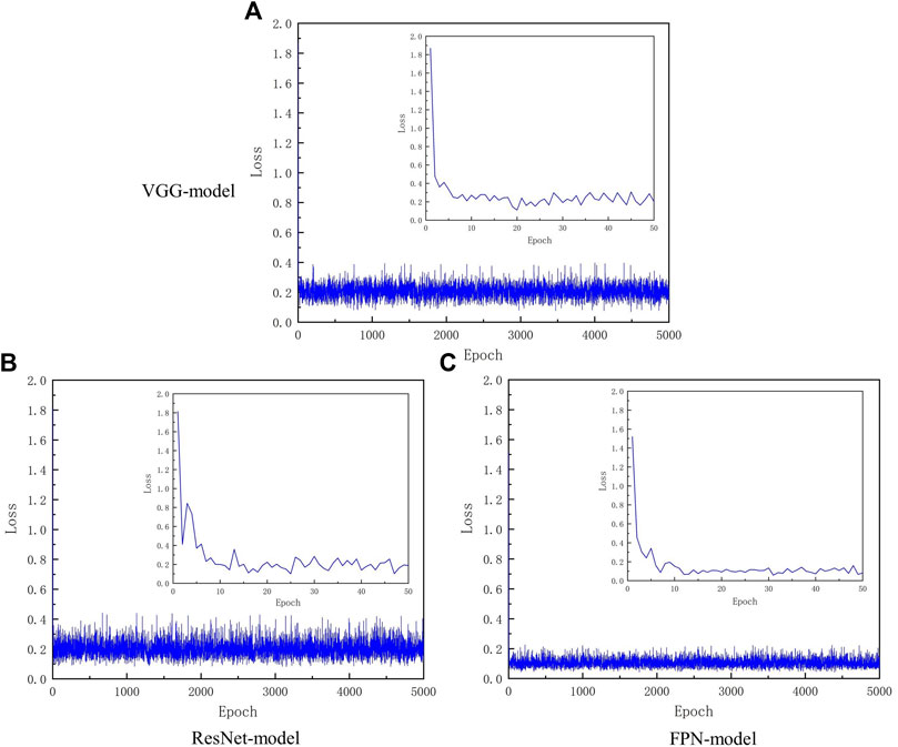
As it has been known, the loss function can extract all aspects of a model down into a single number, which allows the models to be evaluated and compared. Thus, loss value is an indicator for evaluating the performance of a model. For a perfect model, the loss is zero. As shown in Figure 9, if we plot the loss curves as a function of the entire training cycle (5,000 epochs), the variation tendency is compressed and hidden. Thus, the loss was replotted against only 50 epochs for each model (as shown in the small windows) to amplify the changes. The loss values can be used to describe how closely the values predicted by a model match the true values of the problem (Goodfellow et al., 2016). For an ideal model, we can expect a reduction in the loss after each, or several, iteration(s)/epoch(s). For all the models, a sharp drop was found at the first epoch, followed by a gradual decline, eventually leading to stable oscillations. The stable oscillations started between 10 and 20 epochs within small amplitudes and are likely due to the small batch size. Although the small batch size leads to noise in the gradient estimation, the noise is crucial to avoid sharp minima, which could lead to poor generalization for deep learning (Keskar et al., 2016). A lower loss indicates that the model made fewer errors on the data. Thus, the training process finally gives a lower loss, indicating a better model. The lowest average value of the loss, approximately 0.106, in the stably fluctuating region was for the FPN model (as shown in Figure 9).
Calculation Efficiency and Cost
From the perspective of practical applications, the calculation efficiency and cost should be considered, since high requirements in terms of the time consumption, memory cost, and space occupancy would restrict a model when it comes to real-time applications or in the case of devices with a lower calculation capacity.
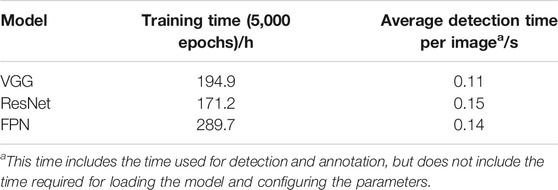
The calculation efficiency is evaluated using the total training time for 5,000 epochs and the average detection time per image (Table 3); the former reflects the time required for training a new model with a new dataset, and the latter can be used to evaluate whether a model can be implemented for instant scenarios, such as on-site detection of FCISs, when using microscopy techniques. The ResNet model required the least amount of training time, approximately 118 h less than that required for training the FPN model. With the GeForce GTX 1060 GPU (6 GB of memory), all the three models could instantaneously make detections within 0.15 s per image, and the VGG model was the fastest in terms of the detection speed. The subtle difference between the average detection time cannot be used as a decisive index for model selection unless a considerable number of images need to be processed.
Table 4 summarizes the memory space and model size required for the training models, pre-trained model sizes, and video memory consumption during detection. The pre-trained model size of the VGG-16 model was nearly three times those of the other two models, leading to a larger final VGG model. Typically, for the same input data, a larger model size means a higher number of parameters in the deep neural network. Canziani et al. (2016) reported that VGG-16 requires more parameters [138 M parameters (Simonyan and Zisserman, 2014)] than ResNet-101 [44.5 M parameters (Yu et al., 2017)] trained on ImageNet and uses larger feature sizes in many layers, making it computationally costly.
Although the FPN and ResNet models have similar sizes, the FPN model required more memory for training, indicating a greater number of computations because of the additional intermediate variables involved. On the other hand, the ResNet model is at a disadvantage in terms of the memory usage for detection, particularly compared with the VGG model.
Summary
The three models were compared in terms of the accuracy, training process, calculation efficiency, and memory cost. The following are their features for FCIS detection:
VGG Model
It was the most expensive model for training and exhibited the lowest performance in terms of the detection accuracy among the three models. It was advantageous in terms of the detection time and memory cost.
ResNet Model
It showed the best performance in terms of the detection accuracy with the minimum model size and training memory cost. The only drawbacks were the relatively high detection memory cost and slightly longer detection time.
FPN Model
Its detection performance was largely similar to that of the ResNet model. However, the model outperformed in terms of the recall. Its calculation cost was quite similar to the ResNet model as well. Thus, if the application requires a higher performance in terms of the recall, this model is superior to the ResNet model. It also performed best for training, as the average loss value was the lowest among the three. However, it was time-consuming for training a new dataset.
The results show that all the three models can be trained thoroughly to obtain good or even desired accuracies for real-time FCIS detection. The relatively complex architecture of the faster R-CNN demands more memory for detection, leading to certain but not extremely high requirements on the processors. In applications for which high-capacity computers are available, e.g., computers attached to microscope for imaging, they can be developed as modules and embedded into the microscope software packages for a quick FCIS detection.
Currently, the fast R-CNN-based models cannot be employed for small devices, such as smartphones, because of the relatively large model size and memory requirement. However, solutions could be developed using simpler algorithms as the backbone and feature extractor, or simply by using a single state-of-the-art algorithm, albeit with a lower detection accuracy, which has been proven in some studies (Canziani et al., 2016; Sehgal and Kehtarnavaz, 2019; Zhang and Deng, 2019; Zhu and Spachos, 2019).
This work has two limitations. The first one is that our training dataset was not general enough to cover all types of fatigue surfaces of metallic compounds. The possible solution to this problem is to collect more annotated data during the implementation of the FCIS detection module and then update the module for improved generalization with the added data. The other limitation is that the number of transfer learning algorithms evaluated was low, hindering the discovery of more possibilities.
Conclusion
This paper presented a comparative work on three transfer learning algorithms using the faster R-CNN as the backbone for detecting FCISs. The three faster R-CNN-based algorithms, namely VGG-16, ResNet-101, and FPN, were used as feature extractors to share the features extracted from ImageNet. All the three models showed remarkable improvements in the detection accuracy compared with our previous study on training a similar model from scratch, indicating the underlying benefits of transferring different semantic features for detecting abstract features such as FCISs. A comparison between the three models in terms of the accuracy, precision, recall, and F1 score showed that the feature extractor with a deeper architecture (ResNet-101) was more efficient in improving the accuracy of the transfer learning models. The overall detection performances of the ResNet and FPN models were similar, with subtle advantages in terms of the precision and recall, respectively. The ResNet model exhibited a better performance in terms of the training time and memory cost compared to the FPN model, whereas the FPN model was better trained because of the lower average loss. Although the VGG model exhibited a lower performance in terms of the detection accuracy among the three, it outperformed the others in terms of the detection time and memory requirement.
Moreover, there was always a tradeoff between the precision and recall. Increasing the confidence threshold value increased the accuracy, precision, and F1 score but reduced the recall. Therefore, the threshold value should be carefully selected depending on the application requirement.
Data Availability Statement
The original contributions presented in the study are included in the article/supplementary material, further inquiries can be directed to the corresponding author.
Author Contributions
SW contributed to conception and design of the study, carried out the experiemts, and wrote the manuscript under the supervision of TG.
Funding
Financial support from Jiangsu Key Research and Development Program (Grant No. BE2019107), the China Postdoctoral Science Foundation (Grant No. 2020M681460), and the Natural Science Foundation of Jiangsu (Grant No. BK20210255) are gratefully acknowledged.
Conflict of Interest
The authors declare that the research was conducted in the absence of any commercial or financial relationships that could be construed as a potential conflict of interest.
Publisher’s Note
All claims expressed in this article are solely those of the authors and do not necessarily represent those of their affiliated organizations, or those of the publisher, the editors and the reviewers. Any product that may be evaluated in this article, or claim that may be made by its manufacturer, is not guaranteed or endorsed by the publisher.
References
Akcay, S., Kundegorski, M. E., Devereux, M., and Breckon, T. P. (2016). “Transfer Learning Using Convolutional Neural Networks for Object Classification within X-ray Baggage Security Imagery,” in Proceedings of the IEEE International Conference on Image Processing, 25-28 Sept. 2016, 1057–1061.
Canziani, A., Paszke, A., and Culurciello, E. (2016). An Analysis of Deep Neural Network Models for Practical Applications. arXiv:1605.07678
Coutinho, E., Deng, J., and Schuller, B. (2014). “Transfer Learning Emotion Manifestation across Music and Speech,” in Proceedings of the International Joint Conference on Neural Networks (IJCNN) (New York: IEEE). doi:10.1109/ijcnn.2014.6889814
Cowles, B. (1996). High Cycle Fatigue in Aircraft Gas Turbines—An Industry Perspective. Int. J. Fracture 80 (2-3), 147–163. doi:10.1007/bf00012667
Deng, J., Dong, W., Socher, R., Li, L., Li, K., and Fei-Fei, L. (2009). “Imagenet: A Large-Scale Hierarchical Image Database,” in Proceedings of the IEEE conference on computer vision and pattern recognition (New York: IEEE). doi:10.1109/cvpr.2009.5206848
Du, J. (2018). Understanding of Object Detection Based on CNN Family and YOLO. J. Phys. Conf. Ser. 1004, 012029. doi:10.1088/1742-6596/1004/1/012029
Fukushima, K. (1980). Neocognitron: A Self-Organizing Neural Network Model for a Mechanism of Pattern Recognition Unaffected by Shift in Position. Biol. Cybernetics 36 (4), 193–202. doi:10.1007/bf00344251
Girshick, R., Donahue, J., Darrell, T., and Malik, J. (2014). “Rich Feature Hierarchies for Accurate Object Detection and Semantic Segmentation,” in Proceedings of the IEEE conference on computer vision and pattern recognition (New York: IEEE). doi:10.1109/cvpr.2014.81
Girshick, R. (2015). “Fast R-Cnn,” in Proceedings of the IEEE international conference on computer vision. doi:10.1109/iccv.2015.169
Guo, T., Liu, Z., Correia, J., and de Jesus, A. M. P. (2020). Experimental Study on Fretting-Fatigue of Bridge cable Wires. Int. J. Fatigue 131, 105321. doi:10.1016/j.ijfatigue.2019.105321
He, K., Zhang, X., Ren, S., and Sun, J. (2016). “Deep Residual Learning for Image Recognition,” in Proceedings of the IEEE conference on computer vision and pattern recognition (New York: IEEE). doi:10.1109/cvpr.2016.90
Hemath, M., Mavinkere Rangappa, S., Kushvaha, V., Dhakal, H. N., and Siengchin, S. (2020). A Comprehensive Review on Mechanical, Electromagnetic Radiation Shielding, and thermal Conductivity of Fibers/inorganic Fillers Reinforced Hybrid Polymer Composites. Polym. Composites 41 (10), 3940–3965. doi:10.1002/pc.25703
Huang, H. M., Tsai, C. M., Chang, C. C., Lin, C. T., and Lee, S. Y. (2005). Evaluation of Loading Conditions on Fatigue-Failed Implants by Fracture Surface Analysis. Int. J. Oral Maxillofac. Implants 20 (6), 854–859.
Hubel, D. H., and Wiesel, T. N. (1962). Receptive fields, Binocular Interaction and Functional Architecture in the Cat's Visual Cortex. J. Physiol. 160 (1), 106–154. doi:10.1113/jphysiol.1962.sp006837
Kaiming, H., Zhang, X., Ren, S., and Sun., J. (2015). Deep Residual Learning for Image Recognition. Available at: https://github.com/KaimingHe/deep-residual-networks.
Keskar, N. S., Mudigere, D., Nocedal, J., Smelyanskiy, M., and Tang, P. T. P. (2016). On Large-Batch Training for Deep Learning: Generalization Gap and Sharp Minima.
Khan, A., Sohail, A., Zahoora, U., and Qureshi, A. S. (2019). A Survey of the Recent Architectures of Deep Convolutional Neural Networks. arXiv preprint arXiv:1901.06032.
Kushvaha, V., Kumar, S. A., Madhushri, P., and Sharma, A. (2020). Artificial Neural Network Technique to Predict Dynamic Fracture of Particulate Composite. J. Compos. Mater. 54 (22), 3099–3108. doi:10.1177/0021998320911418
Kushvaha, V., and Tippur, H. (2014). Effect of Filler Shape, Volume Fraction and Loading Rate on Dynamic Fracture Behavior of Glass-Filled Epoxy. Composites B: Eng. 64, 126–137. doi:10.1016/j.compositesb.2014.04.016
Lecun, Y., Bottou, L., Bengio, Y., and Haffner, P. (1998). Gradient-based Learning Applied to Document Recognition. Proc. IEEE 86 (11), 2278–2324. doi:10.1109/5.726791
Lin, T.-Y., Dollar, P., Girshick, R., He, K., Hariharan, B., and Belongie, S. (2017). “Feature Pyramid Networks for Object Detection,” in Proceedings of the IEEE conference on computer vision and pattern recognition (New York: IEEE). doi:10.1109/cvpr.2017.106
Lucena, O., Junior, A., Moia, V., Souza, R., Valle, E., and Lotufo, R. (2017). “Transfer Learning Using Convolutional Neural Networks for Face Anti-spoofing,” in Proceedings of the International Conference Image Analysis and Recognition, 02 June 2017 (Cham: Springer International Publishing).
Meng, J.-n., Lin, H.-f., and Yu, Y.-h. (2010). “Transfer Learning Based on Svd for Spam Filtering,” in Proceedings of the International Conference on Intelligent Computing and Cognitive Informatics (New York: IEEE). doi:10.1109/icicci.2010.115
Oquab, M., Bottou, L., Laptev, I., and Sivic, J. (2014). “Learning and Transferring Mid-level Image Representations Using Convolutional Neural Networks,” in Proceedings of the IEEE conference on computer vision and pattern recognition (New York: IEEE). doi:10.1109/cvpr.2014.222
Pan, S. J., and Yang, Q. (2009). A Survey on Transfer Learning. IEEE Trans. knowledge Data Eng. 22 (10), 1345–1359.
Pan, W., Zhong, E., and Yang, Q. (2012). “Transfer Learning for Text Mining,” in Mining Text Data (New York: Springer), 223–257. doi:10.1007/978-1-4614-3223-4_7
Park, W. B., Chung, J., Jung, J., Sohn, K., Singh, S. P., Pyo, M., et al. (2017). Classification of crystal Structure Using a Convolutional Neural Network. Int. Union Crystallogr. J. 4 (4), 486–494. doi:10.1107/s205225251700714x
Qian, Y., Dong, J., Wang, W., and Tan, T. (2016). “Learning and Transferring Representations for Image Steganalysis Using Convolutional Neural Network,” in Proceedings of the IEEE International Conference on Image Processing (Phoenix, AZ: ICIP), 2752–2756. doi:10.1109/icip.2016.7532860
Quattoni, A., Collins, M., and Darrell, T. (2008). “Transfer Learning for Image Classification with Sparse Prototype Representations,” in Proceedings of the IEEE Conference on Computer Vision and Pattern Recognition (New York: IEEE). doi:10.1109/cvpr.2008.4587637
Ren, S., He, K., Girshick, R., and Sun, J. (2015). “Faster R-Cnn: Towards Real-Time Object Detection with Region Proposal Networks,” in Advances in Neural Information Processing Systems. 28, 91–99.
Ryan, K., Lengyel, J., and Shatruk, M. (2018). Crystal Structure Prediction via Deep Learning. J. Am. Chem. Soc. 140 (32), 10158–10168. doi:10.1021/jacs.8b03913
Schwarz, M., Schulz, H., and Behnke, S. (2015). “RGB-D Object Recognition and Pose Estimation Based on Pre-trained Convolutional Neural Network Features,” in Proceedings of the IEEE International Conference on Robotics and Automation (Seattle, WA: ICRA). doi:10.1109/icra.2015.7139363
Sehgal, A., and Kehtarnavaz, N. (2019). Guidelines and Benchmarks for Deployment of Deep Learning Models on Smartphones as Real-Time Apps. Machine Learning and Knowledge Extraction 1 (1), 450–465.
Sharma, A., Anand Kumar, S., and Kushvaha, V. (2020). Effect of Aspect Ratio on Dynamic Fracture Toughness of Particulate Polymer Composite Using Artificial Neural Network. Eng. Fracture Mech. 228, 106907. doi:10.1016/j.engfracmech.2020.106907
Sharma, A., and Kushvaha, V. (2020). Predictive Modelling of Fracture Behaviour in Silica-Filled Polymer Composite Subjected to Impact with Varying Loading Rates Using Artificial Neural Network. Eng. Fracture Mech. 239, 107328. doi:10.1016/j.engfracmech.2020.107328
Shen, Z., Liu, Z., Li, J., Jiang, Y., Chen, Y., and Xue, X. (2017). “Dsod: Learning Deeply Supervised Object Detectors from Scratch,” in Proceedings of the IEEE International Conference on Computer Vision (New York: IEEE). doi:10.1109/iccv.2017.212
Simonyan, K., and Zisserman, A. (2014). Very Deep Convolutional Networks for Large-Scale Image Recognition. arXiv: 1409.1556
Song, P., Jin, Y., Zhao, L., and Xin, M. (2014). Speech Emotion Recognition Using Transfer Learning. IEICE Trans. Inf. Syst. E97.D (9), 2530–2532. doi:10.1587/transinf.2014edl8038
Szegedy, C., Vanhoucke, V., Ioffe, S., Shlens, J., and Wojna, Z. (2016). “Rethinking the Inception Architecture for Computer Vision,” in Proceedings of the IEEE conference on computer vision and pattern recognition (New York: IEEE). doi:10.1109/cvpr.2016.308
Talo, M., Baloglu, U. B., Yıldırım, Ö., and Rajendra Acharya, U. (2019). Application of Deep Transfer Learning for Automated Brain Abnormality Classification Using Mr Images. Cogn. Syst. Res. 54, 176–188. doi:10.1016/j.cogsys.2018.12.007
Wang, S. Y., Zhang, P. Z., Zhou, S. Y., Wei, D. B., Ding, F., and Li, F. K. (2020). A Computer Vision Based Machine Learning Approach for Fatigue Crack Initiation Sites Recognition. Comput. Mater. Sci. 171, 109259. doi:10.1016/j.commatsci.2019.109259
Weiss, K., Khoshgoftaar, T. M., and Wang, D. (2016). A Survey of Transfer Learning. J. Big Data 3 (1), 9. doi:10.1186/s40537-016-0043-6
Xie, T., and Grossman, J. C. (2018). Crystal Graph Convolutional Neural Networks for an Accurate and Interpretable Prediction of Material Properties. Phys. Rev. Lett. 120 (14), 145301. doi:10.1103/physrevlett.120.145301
Yang, J., Lu, J., Batra, D., and Parikh, D., (2017). A Faster Pytorch Implementation of Faster R-Cnn. Available at: https://github.com/jwyang/faster-rcnn.pytorch
Zeiler, M. D., and Fergus, R. (2014). “Visualizing and Understanding Convolutional Networks,” in European Conference on Computer Vision (New York: Springer). doi:10.1007/978-3-319-10590-1_53
Zhang, H., and Deng, Q. (2019). Deep Learning Based Fossil-Fuel Power Plant Monitoring in High Resolution Remote Sensing Images: A Comparative Study. Remote Sensing 11 (9), 1117. doi:10.3390/rs11091117
Zhu, L., and Spachos, P. (2019). Towards Image Classification with Machine Learning Methodologies for Smartphones. Mach. Learn. Knowl. Extr. 1 (4), 1039–1057. doi:10.3390/make1040059
Zhu, Y., Chen, Y., Lu, Z., Pan, S. J., Xue, G-R., Yu, Y., et al. (2011). “Heterogeneous Transfer Learning for Image Classification,” in Proceedings of the Twenty-Fifth AAAI Conference on Artificial Intelligence, San Francisco, CA, August 7–11, 2011.
Keywords: computer vision, machine learning, transfer learning, fatigue crack initiation sites, faster R-CNN
Citation: Wang SY and Guo T (2021) Transfer Learning-Based Algorithms for the Detection of Fatigue Crack Initiation Sites: A Comparative Study. Front. Mater. 8:756798. doi: 10.3389/fmats.2021.756798
Received: 11 August 2021; Accepted: 28 October 2021;
Published: 23 November 2021.
Edited by:
Tanmoy Mukhopadhyay, Indian Institute of Technology Kanpur, IndiaReviewed by:
Vinod Kushvaha, Indian Institute of Technology Jammu, IndiaSathiskumar Anusuya Ponnusami, City University of London, United Kingdom
Copyright © 2021 Wang and Guo. This is an open-access article distributed under the terms of the Creative Commons Attribution License (CC BY). The use, distribution or reproduction in other forums is permitted, provided the original author(s) and the copyright owner(s) are credited and that the original publication in this journal is cited, in accordance with accepted academic practice. No use, distribution or reproduction is permitted which does not comply with these terms.
*Correspondence: T. Guo, Z3VvdG9uZ0BzZXUuZWR1LmNu
 S.Y. Wang
 T. Guo*