Prediction of Inclusion Types From BSE Images: RF vs. CNN

The analysis of non-metallic inclusions is crucial for the assessment of steel properties. Scanning electron microscopy (SEM) coupled with energy dispersive spectroscopy (EDS) is one of the most prominent methods for inclusion analysis. This study utilizes the output generated from SEM/EDS analysis to predict inclusion types from BSE images. Prediction models were generated using two different algorithms, Random Forest (RF) and convolutional neural networks (CNN), for comparison. For each method, three separate models were developed. Starting with a simple binary model to differentiate between inclusions and non-inclusions, then developing to more complex four and five class models. For the 4-class model, inclusions were split into oxides, sulfides, and oxy-sulfides, in addition to the non-inclusion class. The 5-class model included specific types of inclusions only, namely alumina, calcium aluminates, calcium sulfides, complex calcium-manganese sulfides, and oxy-sulfide inclusions. CNN achieved better accuracy for the binary (92%) and 4-class (78%) models, compared to RF (binary 87%, 4-class 75%). For the 5-class model, the results were similar, 60% accuracy for RF and 59% for CNN.

Introduction

Steel production methods have consistently evolved toward producing material with lower impurity levels and better properties. Efforts in this area are generally referred to as “clean steel” production, with the level of cleanliness required depending on the product requirements. It is generally accepted that clean steels have a low frequency of product defects due to the presence of non-metallic inclusions (Cramb and Briant, 1999). Non-metallic inclusions are oxide, sulfide, or nitride particles that are present in the liquid metal. They form due to chemical reactions occurring during steelmaking and by entrainment of oxide slag and refractory materials. Inclusions are generally considered detrimental to downstream steel processing and product performance, though in some cases they are engineered to improve steel properties (Abraham et al., 2018), (Holappa and Wijk, 2014). Examples of the detrimental effects of inclusions include the reduction of fatigue resistance, strength, ductility, or fracture strength (Atkinson and Shi, 2003; Garrison and Wojcieszynski, 2007; Garrison and Wojcieszynski, 2009; Gupta et al., 2015). Therefore, the analysis of non-metallic inclusions is crucial for the assessment of steel properties.

The current state-of-the-art method for analysis of non-metallic inclusions utilizes automated scanning electron microscopy (SEM) along with energy dispersive x-ray spectroscopy (EDS) (Goransson et al., 1999; Zhang and Thomas, 2003a; Story and Asfahani, 2013; Harada et al., 2014). SEM/EDS analysis enabled the analysis of hundreds or thousands of inclusions in a matter of hours of less. Inclusion size can have drastic effects on the mechanical properties of the final product. Moreover, different types of inclusions have varying effects on steel (Atkinson and Shi, 2003), (Garrison and Wojcieszynski, 2009), (Zhang and Thomas, 2003a), (Zhang and Thomas, 2003b), (Ånmark et al., 2015). Therefore, inclusion SEM/EDS analysis has been generally focused on inclusion size, total amount, and chemical composition. The method generates an abundance of raw output data on each particle analyzed, including the spatial position, chemical composition, size, and morphological features of each particle analyzed, in addition to a magnified backscattered electron (BSE) image of the particle.

Automated SEM/EDS is still too slow to serve as an online production monitoring tool and typically averaged quantities are output and analyzed by engineers and operators. In this work, we investigate the use of machine learning and computer vision methods to extract information on inclusion chemical composition from BSE SEM images. In other fields, machine learning has gained a great deal of attention especially with the considerable processing power of modern computers (James et al., 2013). Machine learning utilizes data to teach a computer system how to infer or predict decisions without being explicitly programmed to do so. Such techniques have been recently applied in the steel industry. Most of the current work has been focused on utilizing computer vision for the detection of surface defects and scratches (Wang et al., 1883; Konovalenko et al., 2021; Zhao et al., 2021). The focus of the work presented here is to utilize machine learning to predict inclusion types from their BSE images. Inclusion types are generally specified based on user defined criteria applied to the compositional measurements generated from x-ray signals (EDS analysis). While BSE images are generated by raster scanning an inclusion and measuring the BSE yield (i.e. BSE signal) to produce a greyscale image of the particle. The amount of BSE yield is directly related to the mass averaged atomic number of the material analyzed (Goldstein et al., 2018). This leads to different grey level contrast between different materials, as a result inclusions can be clearly identified from the steel matrix in an SEM. Since both BSE and x-ray signals are related to composition, machine learning can be applied to predict one signal from the other.

Throughout the secondary metallurgy processes, several steel samples are taken for SEM/EDS analysis to monitor inclusions and ensure their conformity with the specified requirements. Although the analysis is conducted offline, conducting the analysis in a timely manner is critical. By predicting inclusion types from their BSE images, SEM/EDS analysis time can be reduced by mitigating the need for EDS analysis. The prediction models rely heavily on the availability of training data, and this is readily available in steel plants where the same grade of steel is continuously produced and analyzed on a daily basis.

The method utilized is referred to as supervised learning. With supervised learning algorithms, a relationship between inputs and outputs is formulated based on some available data, known as the training data. When new data is presented, the output is predicted based on the relationship developed from the training data (Bishop, 2006). The task at hand is a classification problem since the output variable (inclusion type) is a discrete categorical variable. There are numerous supervised learning algorithms available, each having their own pros and cons. In this study, two specific algorithms were selected and compared, the Random Forest (RF) algorithm and Convolutional Neural Networks (CNN). For both methods, the approach was to develop three separate models. The first model was a binary model to classify “inclusions” from “non-inclusions”. The second model, a 4-class model, which includes “non-inclusions” and a breakdown of inclusions into types: “oxides”, “sulfide”, and “oxy-sulfides.” The last model was a 5-class model, to predict specific inclusion types.

Materials and Methods

The inclusion dataset utilized in this study was compiled from four final plate product samples. All were from different heats that were Al-deoxidized and Ca-treated. The SEM analysis was carried out at 20 kV accelerating voltage, using the Automated Steel Cleanliness Analysis Tool (ASCAT) (Story et al., 2005). The EDS analysis was conducted using point mode, i.e. x-rays are collected from a single point on the particle which is assumed to be the center of the particle. As per the SEM setting of the sample supplier, the Fe content was not included in the EDS analysis. BSE images (128 × 128 pixels) were also provided for each feature analyzed. Inclusions were mostly composed of Ca-Al-S, with minor amounts of Mn. It was assumed that all Mn would be in the form of MnS, the remaining S would be in CaS, and all other inclusions would be in the form of oxides. The reference greyscale value (GSV) utilized in the analysis were 200 for Fe and 50 for Al. The measurement GSV threshold were set to 0–170, i.e., only particles with a GSV less than 170 were analyzed. The total number of particles analyzed was 29,318 particles.

Three separate models were developed to predict inclusion classes, starting with a simple binary model, then expanding to more specific four and five class models. Specific definitions of the classes are provided below. The aim of utilizing these three models was to gradually increase the complexity of each model and evaluate its effect on the overall prediction accuracy.

To allow for a justifiable comparison between different prediction models, a standardized labelling criteria was devised to classify inclusions based on their EDS measurements. Each particle is initially classified as an inclusion or non-inclusion based on the Fe and Si content. High Fe content is associated with pores on the surface of the sample, and the only source of Si is assumed to be from contaminants on the surface of the sample. However, since the Fe content was not analyzed in the available dataset the total x-ray counts were utilized instead. Therefore, any particle with less than 3,000 total x-ray counts or more than 10 Si at% were labelled as non-inclusions, all other particles were labelled as inclusions. It should be noted that this classification scheme does not pertain to Si deoxidized steels where Si containing inclusions are expected to be present.

The relevant inclusion composition variables (Mg, Al, Ca, S, Mn, and Ti) were then normalized, and inclusions were broken down into several types based on the following criteria (all percentages are atomic percentages):

• Oxide: (Mg + Al + Ca-S) > 80% and S < 10%

• Sulfide: (Ca + Mn + S) > 80% and (Mg + Al) < 10%

• Oxy-sulfide: S > 10% and (Mg + Al + Ca-S) > 10%

• Nitride: Ti > 80%

• Other: remainder

Oxide and sulfide inclusion were further divided into more specific classes, as follows:

Oxides

Al₂O₃: Al > 80%

MgAl₂O₄: (Mg + Al) > 80% and 0.25 < Mg/Al < 0.75

CA (calcium aluminates): (Ca + Al) > 80% and 0.1 < Ca/Al <3.2

CaO: Ca > 80%

Other oxides: remainder

Sulfides

CaS: Mn < 10%

MnS: Ca < 10%

CaS-MnS: remainder

The ratios used for the classification of MgAl₂O₄ and CA inclusions were based on their stoichiometric ratios. The CA inclusion class pertains to all types of calcium aluminates (commonly referred to as C3A, C12A7, CA, CA2, and CA6).

A breakdown of the inclusion types in the dataset is given in Table 1.

TABLE 1

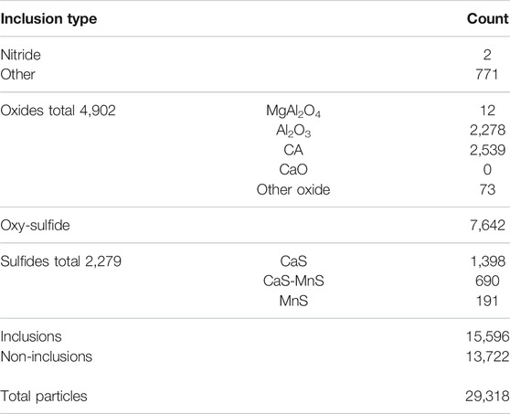
TABLE 1. Breakdown of inclusion types in available dataset.

The binary model predicts whether a BSE image is of an inclusion or a non-inclusion. The 4-class model includes the non-inclusion class and a breakdown of the inclusion class into oxides, sulfides, or oxy-sulfides. And finally, the 5-class model focuses on specific inclusion classes: alumina (Al₂O₃), calcium aluminates (CA), oxy-sulfides, calcium sulfides (CaS), and complex calcium-manganese sulfides (CaS-MnS). These specific inclusion classes were selected based on their abundance in the dataset.

For each prediction model, the data is initially filtered to include the relevant classes with an equal number of observations in each class (i.e. balanced data). Therefore, the total number of observations for each model was dependent on the smallest class size. Table 2 summarizes the classes in each model, along with the limiting class size.

TABLE 2

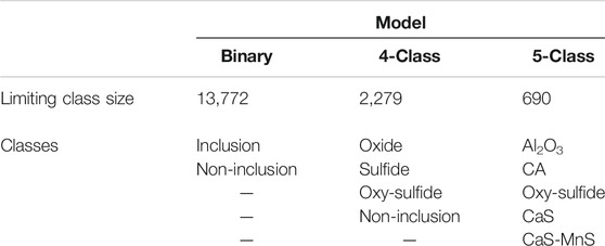
TABLE 2. Summary of inclusion models, relevant classes, and limiting class size.

The dataset was then broken down into a training, validation, and testing datasets. The training datasets was composed of 60% of the data, and the validation and testing datasets were 20% each. Several models are trained (on the training dataset) using a wide range of parameters and evaluated on the validation dataset. This process was carried out to obtain the optimal parameters, based on the highest prediction accuracy. The prediction accuracy is defined as the percentage of correctly predicted images (i.e. percentage of true positive and true negatives). Once the parameters were selected, the final model is trained on both the training and validation datasets (80% of the data) and evaluated on the testing dataset, to obtain the final prediction result. Since this is a classification task, the prediction accuracy is defined as the sum of correctly classified data points divided by the total number of points. The sampling of training and testing data was held constant for both all RF and CNN models, to ensure consistency.

The RF algorithm (Breiman, 2001) was derived from an earlier form of supervised learning, decision trees (Breiman et al., 1984). Decision trees recursively split the data to produce a flowchart with a tree-like structure. The tree is generated based on the training data, starting with the root node on top, branching out into several other nodes, and eventually reaching the terminal nodes. Each node designates a split in the dataset based on one of its input variables, and the terminal nodes identify the predicted class. With the RF algorithm numerous trees are generated from subsets of the data, thereby reducing the overall bias in the data. This leads to better prediction accuracy compared to a decision tree (James et al., 2013).

For the RF prediction models, BSE images were converted to raw numerical data and appended to the inclusion data. The conversion is a tabulated histogram, identifying the number of pixels from the BSE image for each GSV. Therefore, each BSE image is described by 256 variables (i.e., GSVs from 0 to 255), the value for each variable corresponds to the number of pixels with the specified GSV in the BSE image. An example is given below in Figure 1. The histogram displays the number of pixels for each GSV in the BSE image. The inclusion BSE image from which the histogram is generated is shown on the top-left corner of the figure. Therefore, the inputs for the RF models are the GSV variables (the “predictor” variables), and the output is the inclusion classification (the “target” variable). All RF models were conducted in R, an open source programming software.

FIGURE 1

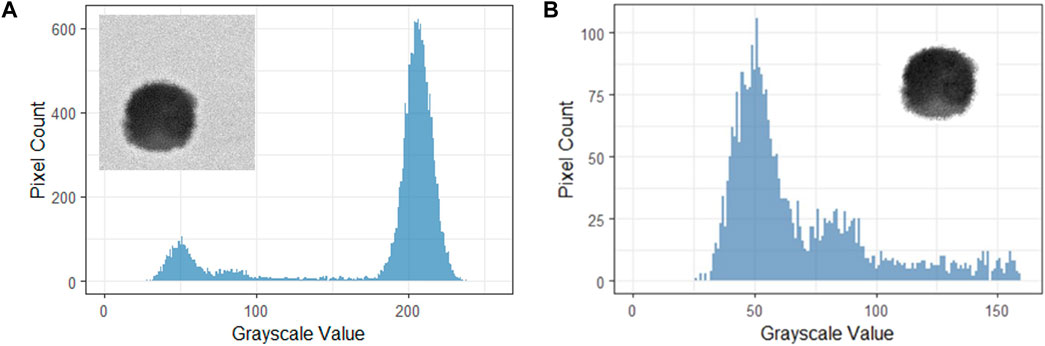
FIGURE 1. Example of GSV histogram of an inclusion BSE image. The BSE image is displayed on the top left corner.

The second method utilized for inclusion classification is a convolutional neural network (CNN) (Schmidhuber, 2015). In contrast to RF, which is used for tabulated data, CNN is an artificial neural network used for image analysis. CNNs are a type of deep machine learning algorithm that perform very well at image classification tasks. A CNN passes the original image through multiple filter banks to create a multiscale representation of the image in the form of a high dimensional vector. The system then uses a classifier (typically a multilayer perceptron) that identifies the probability that an image belongs to a given class. Both the filters and the classifier are learned from the training data, and then can be used to classify additional images.

One of the main drawbacks of CNNs is the preprocessing required to develop the ideal model. Defining the CNN’s architecture can be an arduous task, i.e., selecting the number of hidden layers, number of neurons per layer, activation function, weights … etc. Fortunately, there are various well-established architectures available that can be used, and even be modified or tailored, for image classification, such as ResNet, AlexNet, VGG, LeNet and others.

VGG16 (Simonyan and Zisserman, 2015), a powerful CNN which performs well at the ImageNet Dataset (Deng et al., 2009) natural image classification task, was utilized for inclusion classification. VGG16 was slightly modified, with architecture shown in Figure 2. Standard VGG16 contains five convolutional blocks and three fully connected layers (FCLs). Convolution layers in convolutional blocks are filters to summarize the presence of features in an input. Pooling layers are used to downscale feature maps by summarizing the presence of features in patches of the feature map. Highly condensed features are finally flattened to pass through fully-connected layers for classification tasks. A fully-connected layer multiplies the input by a weight matrix and then adds a bias vector. This provides a computationally cheap and convenient way of learning non-linear combinations of these features.

FIGURE 2

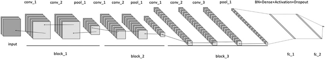
FIGURE 2. Modified VGG16 architecture used in this work.

The modified architecture discards deeper layers from block_4 in the original VGG16. The pretrained layers and their associated parameters from block_1 to block_3 are retained without further training. The outputs from block_3—conv_3 were utilized as characteristic features to perform classification tasks. Two fully-connected layers fc_1 and fc_2 are designed to recognize non-inclusions and the different inclusion classes. The features extracted from the modified VGG16 architecture were generated from conv_3 layer. Instead of training from scratch, feature extraction was initialized with a pre-trained VGG-16 network trained on the ImageNet. The size of input images was 128 × 128 pixels. To prevent overfitting, a combination of Batch Normalization (BN) and Dropout regularization was utilized. Adam optimizer is used with the learning rate of 0.001 for 10 epochs of training. All programming for the CNN models was carried out in python.

Results

Three BSE image examples for each of the selected inclusions classes are given in Figure 3, based on the specified labelling criteria. The figure displays some of the variations in GSV and particle morphology between different classes.

FIGURE 3

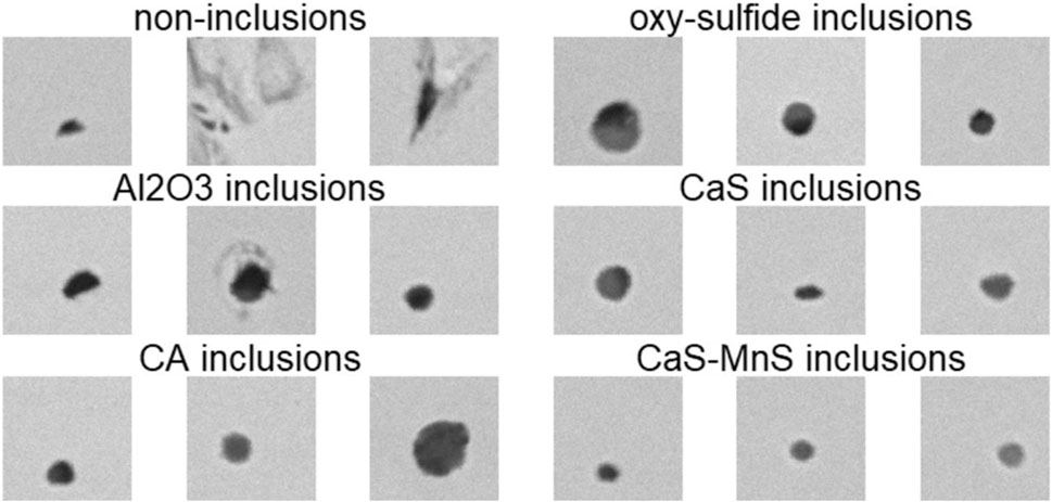
FIGURE 3. Three BSE image examples for each of the selected inclusion classes.

For RF classification the main parameters are the number of trees, number of variables per tree, and the minimum number of observations in the terminal nodes. To select the ideal parameters the model was trained and tested on several parameter ranges for each of the separate models.

The selected range of parameters were as follows:

• Number of trees: 500–1,500

• Variables per tree: 50–100

• Minimum node size: 10–100

The variation in accuracy was relatively low for the range of parameters selected. The difference between lowest and highest validation data accuracy was 5% for the 5-class model, 3% for the 4-class model, and 2% for the binary model. The accuracy did not decrease significantly unless relatively low number of trees or variables per trees were selected, or a high minimum node size was selected. The adopted parameters were 500 trees, with 60 variables per tree, and a minimum of 10 data points in the terminal nodes.

A limiting factor with regards to supervised learning is the number of observations used to train the model. Figure 4 illustrates the relationship between the size of the data and testing accuracy, using RF classification. Models were trained using various numbers of observations, to assess the effect on accuracy. In addition, three trials were conducted for each number of observations, to quantify any uncertainty in the accuracy. Figure 4 displays the averaged test accuracy against the total number of observations (training + testing data) used in the model. For each model, the specified number of observations was randomly selected from the specified classes, the model was trained on 80% of these observations, and the accuracy corresponds to prediction results on the remaining 20% of the data. For example, for a 4-class model with a total of 8,000 observations, the model is trained on 6,400 observations and the accuracy is the prediction result on the withheld 1,600 observations. The same process is reiterated three times, on each run the specified number of observations is randomly selected from the available data. The error bars represent the maximum and minimum accuracies for the three trials. As the number of observations is increased, a steady increase in accuracy is shown for the four and five class models. Whereas, for the binary model the testing accuracy fluctuates around 86.5% when 6,000 observations or more are used. Therefore, it can be safely assumed that enough data is available for the binary model, but not for the four and five class models. This was also displayed with the CNN models as shown in training history curves in Figure 5, illustrating the accuracy and loss against the number of epochs. For the four and five class models, all the available The binary model provided a suitable case to assess the tradeoffs between accuracy, number of observations, and training time. A summary of the results is presented in Figure 6, displaying the average training time (figure a) and testing accuracy (figure b), from the three trials, with respect to the total number of observations in the training data for the binary model. The error bars represent the maximum and minimum of the three trials.

FIGURE 4

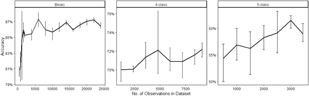
FIGURE 4. Averaged testing accuracy as a function of number of observations used for each model. For each specified number of observations, three trials were conducted. The error bars represent the maximum and minimum errors.

FIGURE 5

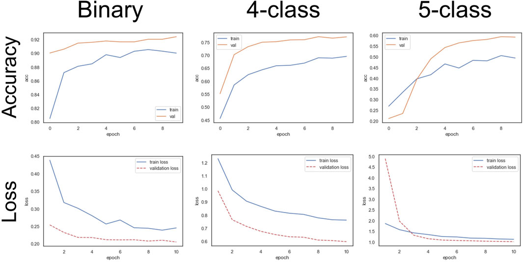
FIGURE 5. CNN binary, 4-class, and 5-class models accuracy and loss curves for training and validation datasets.

FIGURE 6

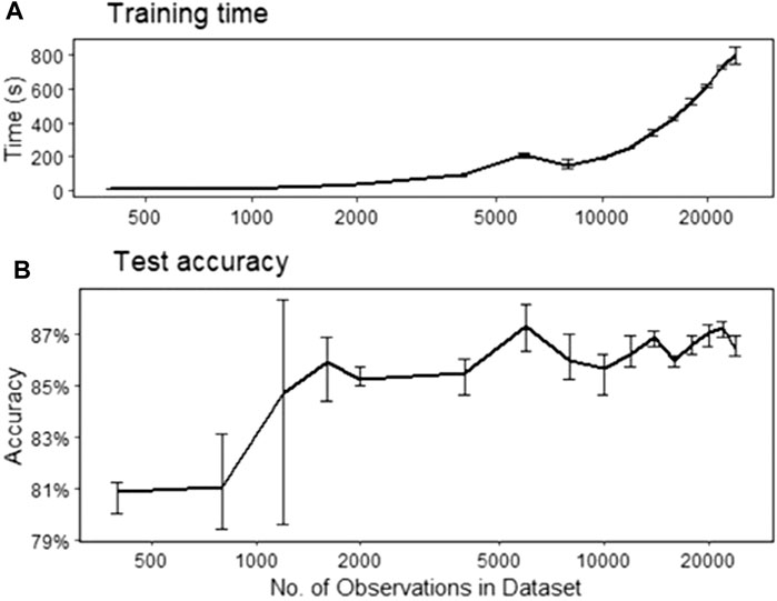
FIGURE 6. Number of observations in training data vs training time (A) and testing accuracy (B). Error bars represent minimum and maximum of three trials. Note: the horizontal axis is in log scale.

The prediction accuracies for all three models are summarized in Table 3 for both RF and CNN. The prediction accuracy is defined as the correctly predicted particles (sum of true positives and true negatives) divided by the total number of particles in the respective testing data.

TABLE 3

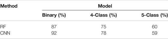
TABLE 3. Testing accuracy results of RF and CNN on all three models.

A visual comparison between the prediction results for both RF and CNN methods is given in Figure 7. The prediction results for each combination of model and method are displayed as confusion matrices, where the rows and columns of each matrix correspond to the actual and predicted labels, respectively. The color of the squares represents the percentage of observations within each class, i.e., a confusion matrix with red diagonal squares and white off-diagonals signifies a 100% accuracy. The last column in the matrix displays the in-class accuracy. The top row of confusion matrices corresponds to RF predictions, the bottom to CNN predictions, and the columns to the three different models.

FIGURE 7

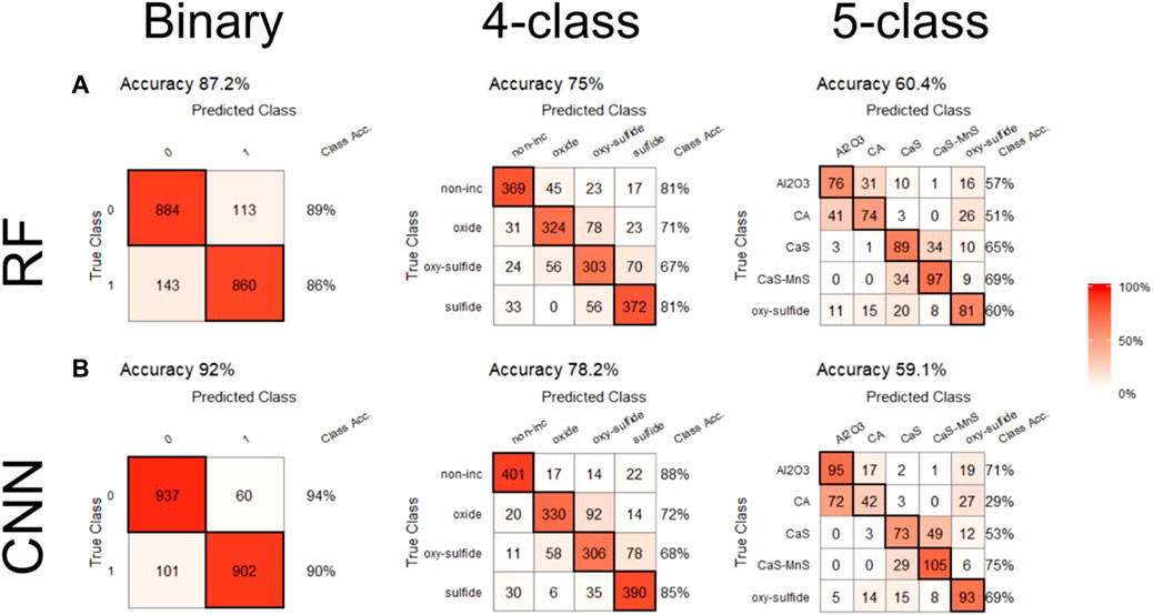
FIGURE 7. Confusion matrices for prediction results of all three models using RF (A) and CNN (B).

Discussion

For the four and five class models, the limiting factor was the availability of training data, as displayed in Figure 4. On the other the hand, there was an abundance of data for the binary model. This presented an opportunity to assess the relationship between number of observations, accuracy, and training time, and obtain an estimate on the adequate number of observations required for classification prediction. As shown in Figure 6, there is a significant increase in accuracy (∼5%) when the training data is increased from a few hundred observations to a few thousand observations. Moreover, the uncertainty in prediction accuracy decreases as more observations are used for training. From this figure, a suitable number of observations can be estimated for RF classification. Although there was some fluctuation in accuracy, the variation in accuracy beyond 6,000 observations was within 1%. Therefore, it can be implied that for the binary model 6,000 observations (i.e., 3,000 observations per class) is sufficient for the purpose of inclusion classification.

The same trend in accuracy was noted for both the RF and CNN models. As the number of classes in a model increases the accuracy decreases. This trend is expected since the models are more specific in terms of inclusion type. This is also due to decreasing number of training data with larger class models. With regards to the binary model, CNN (92%) produced better results compared to RF (87%). This was also observed for the 4-class model (CNN 78%, RF 75%). However, for the 5-class model the RF and CNN produced similar results, 60 and 59% accuracy, respectively.

The confusion matrices in Figure 7 provide an illustration of the uncertainty in the algorithms. For the 4-class model, most errors were made between “oxide”/“oxy-sulfide” and “sulfide”/“oxy-sulfide” inclusions. For the 5-class models, most errors occurred within the oxides or sulfides (i.e., between “Al2O3”/“CA” or “CaS”/“CaS-MnS”). These observations were evident for both the RF and CNN. Therefore, both methods had the same prediction errors. This implies that the errors are due to the similarity in the inclusion BSE images between specific inclusion types (i.e., “Al₂O₃” and “CA”, “CaS” and “CaS-MnS”, “oxides” and “oxy-sulfides”, or “sulfides” and “oxy-sulfides”), and not due to an inherent issue in the methodology. Such errors are expected, since the GSVs of that certain inclusion types are similar, such as Al₂O₃ and CA or CaS and CaS-MnS, and are hard to distinguish on BSE images. Whereas differences between BSE images of non-inclusions, oxides, and sulfides can be arguably easier to identify visually.

Although the CNN method displayed a better result for the binary and 4-class models, the overall difference in prediction accuracy between the CNN and RF for the four and five class models was not significant. CNNs are generally expected to perform better than RF classification for image classification tasks. One reason for this is that the CNNs utilize shape or morphology information as an input, in addition to the different GSVs. With the RF classification method utilized here, the image was converted to tabulated data (histogram of GSVs) which led to information loss (i.e. particle shape was not considered in the analysis). The better accuracy achieved using the CNN compared to RF, implies that there is a significant difference in shape between inclusions and non-inclusions in the training data utilized which was captured by the CNN. Whereas, between different inclusion types, inclusion morphology did not vary as much.

Moreover, because CNNs create a comprehensive representation of image data that captures multiple levels of visual information, their maximum classification accuracy will tend to be larger than RF methods. However, this increased performance comes at a price. Due to the larger number of model parameters that must be optimized, the computational cost of training a CNN model is high, and the input data requirements are large. In addition, in deep learning models such as CNNs, the basis for classification can be difficult or impossible to extract, whereas the individual decision trees in RF models can be analyzed to determine which features of the input data are salient to accurate predictions.

Another consideration is the reliability of the EDS measurements, from which the ground truth image labels are specified. For this dataset, measurements were taken using point mode. Thus, the composition measurement pertains to a specific location on the inclusion, which is generally assumed to be the center of the inclusion. This might not always be the case due to drift in BSE imaging. Moreover, the point at which the EDS is measured might not interact with other phases present in the inclusion. If all inclusions were single phased this will not be an issue, however, a large number of BSE images in this dataset showed multiphase inclusions (e.g., oxy-sulfide inclusions). The BSE image on the other hand, incorporates a better overall picture of the phase distribution. Figure 8 present examples of such cases, where the BSE images clearly show two distinct phases, while the EDS (composition bar to the right of the image) measures only one phase. Conducting EDS measurements using raster mode can help mitigate these errors, however, it will increase the analysis time significantly.

FIGURE 8

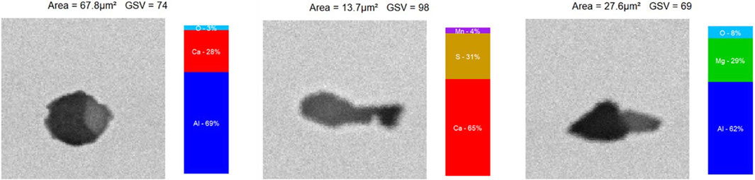
FIGURE 8. Example of multiphase inclusions, with EDS measurement (composition bar) detecting only one phase.

The standardized classification criteria can also pose another source of error. It is devised from a set of objective rules, which is usually the case in industry. The criteria defined in this work sets a minimum threshold of 10%, to allow for some margin of error, when defining certain inclusion types. Figure 9 displays some examples of inclusions classified as “CA” by the standardized criteria, while their BSE image clearly display two phases (these are likely oxy-sulfide phases). This is due to the S content being lower than the minimum threshold of 10%, as shown by the composition bar next to the BSE images.

FIGURE 9

FIGURE 9. Examples of inclusions classified as “CA” by standardized criteria but predicted as “oxy-sulfide.” Composition bar is displayed to the right of each BSE image.

The reliability of EDS measurement and classification criteria are crucial for the formation of reliable prediction models. Studies have been conducted to develop better methods for inclusion EDS measurement. Shah et al. (Shah et al., 2018) proposed the use of phase discrimination on the BSE image to identify different phases, and analyze each phase separately. A similar approach can be adopted to identify the different number of phases and use this as an initial rule for classifying inclusion (e.g., only two-phase inclusion can be oxy-sulfides, one-phase inclusions can be alumina, CaS … etc.). As shown above, most of the errors in both the RF and CNN were due to mislabeled inclusions (e.g. multiphase oxy-sulfides labelled as oxides or sulfides based on EDS measurement, or vice versa). Therefore, the performance of the prediction models relies heavily on the availability and reliability of training data.

Conclusion

RF and CNN models were applied to predict inclusion types from BSE images. Three models were assessed and compared using both methods.

• For the binary classification model (inclusion vs non-inclusion), approximately 3,000 observations per class should be sufficient for training data.

• The binary model had the highest testing accuracy: 87% using the RF, and 92% using CNNs. As the number of classes increases, the accuracy decreased.

• CNN achieved better accuracy for the binary (92%) and 4-class (78%) models, compared to RF (binary 87%, 4-class 75%). For the 5-class model, RF (60%) had slightly better accuracy than CNN (59%).

• The same prediction errors were observed for both RF and CNN. Most of the errors were made between similar inclusion types.

• Reliable EDS measurement and accurate labelling of inclusions are vital for the formation of robust classification prediction models.

Data Availability Statement

The datasets presented in this article are not readily available because permission is required from the sample supplier from which the data was collected. Requests to access the datasets should be directed to mabdulsa@andrew.cmu.edu.

Author Contributions

MA and NG performed all the data analysis in the study. BW and EH provided the concept and supervised the whole work. MA wrote the first draft. All authors revised and edited the manuscript.

Funding

This work was supported in part by the National Science Foundation under grant CMMI-1826218.

Conflict of Interest

The authors declare that the research was conducted in the absence of any commercial or financial relationships that could be construed as a potential conflict of interest.

Publisher’s Note

All claims expressed in this article are solely those of the authors and do not necessarily represent those of their affiliated organizations, or those of the publisher, the editors and the reviewers. Any product that may be evaluated in this article, or claim that may be made by its manufacturer, is not guaranteed or endorsed by the publisher.

Acknowledgments

The authors would also like to acknowledge the support of the members of Center of Iron and Steelmaking Research.

References

Abraham, S., Bodnar, R., Raines, J., and Wang, Y. (2018). Inclusion Engineering and Metallurgy of Calcium Treatment. J. Iron Steel Res. Int. 25, 133–145. doi:10.1007/s42243-018-0017-3

CrossRef Full Text | Google Scholar

Ånmark, N., Karasev, A., and Jönsson, P. (2015). The Effect of Different Non-metallic Inclusions on the Machinability of Steels. Materials 8 (2), 751–783. doi:10.3390/ma8020751

PubMed Abstract | CrossRef Full Text | Google Scholar

Atkinson, H. V., and Shi, G. (2003). Characterization of Inclusions in Clean Steels: A Review Including the Statistics of Extremes Methods. Prog. Mater. Sci. 48 (5), 457–520. doi:10.1016/s0079-6425(02)00014-2

CrossRef Full Text | Google Scholar

Bishop, C. M. (2006). Pattern Recognition and Machine Learning, vol. 4. New York: Springer.

Google Scholar

Breiman, L., Friedman, J., Stone, C. J., and Olshen, R. A. (1984). Classification and Regression Trees. CRC Press.

Google Scholar

Breiman, L. (2001). Random Forests. Mach. Learn. 45 (1), 5–32. doi:10.1023/a:1010933404324

CrossRef Full Text | Google Scholar

Cramb, A. W. (1999). “High Purity, Low Residual, and Clean Steels,” in Impurities In Engineering Materials: ImPatt, Reliability, & Control. Editor Clyde. Briant (New York, NY: CRC Press), 15, 41.

Google Scholar

Deng, J., Dong, W., Socher, R., Li, L.-J., Li, Kai., Fei-Fei, Li., et al. (2009). A Large-Scale Hierarchical Image Database, in Proceedings of the 2009 IEEE Conference on Computer Vision and Pattern Recognition, 2009, Miami, FL, USA, IEEE, 248–255.

Google Scholar

Garrison, W. M., and Wojcieszynski, A. L. (2007). A Discussion of the Effect of Inclusion Volume Fraction on the Toughness of Steel. Mater. Sci. Eng. A. 464 (1–2), 321–329. doi:10.1016/j.msea.2007.02.015

CrossRef Full Text | Google Scholar

Garrison, W. M., and Wojcieszynski, A. L. (2009). A Discussion of the Spacing of Inclusions in the Volume and of the Spacing of Inclusion Nucleated Voids on Fracture Surfaces of Steels. Mater. Sci. Eng. A. 505 (1–2), 52–61. doi:10.1016/j.msea.2008.11.065

CrossRef Full Text | Google Scholar

James, G., Witten, D., Hastie, T., and Tibshirani, R., An Introduction to Statistical Learning, vol. 103. New York, NY: Springer, 2013..

Google Scholar

Goldstein, J. I., Newbury, D. E., Michael, J. R., Ritchie, N. W. M., Scott, J. H. J., and Joy, D. C. (2018). Scanning Electron Microscopy and X-Ray Microanalysis. Springer.

Google Scholar

Goransson, M., Reinholdsson, F., and Willman, K. (1999). Evaluation of Liquid Steel Samples for the Determination of Microinclusion Characteristics by Spark-Induced Optical Emission Spectroscopy. Iron Steelmak. 26 (5), 53–58.

Google Scholar

Gupta, A., Goyal, S., Padmanabhan, K. A., and Singh, A. K. (2015). “Inclusions in Steel: Micro–macro Modelling Approach to Analyse the Effects of Inclusions on the Properties of Steel. Int. J. Adv. Manuf. Technol. 77 (1–4), 565–572. doi:10.1007/s00170-014-6464-5

CrossRef Full Text | Google Scholar

Harada, A., Maruoka, N., Shibata, H., Zeze, M., Asahara, N., Huang, F., et al. (2014). Kinetic Analysis of Compositional Changes in Inclusions during Ladle Refining. ISIJ Int. 54 (11), 2569–2577. doi:10.2355/isijinternational.54.2569

CrossRef Full Text | Google Scholar

Holappa, L., and Wijk, O. (2014). “Inclusion Engineering,” in Treatise On Process Metallurgy. Elsevier, 347–372. doi:10.1016/b978-0-08-096988-6.00008-0

CrossRef Full Text | Google Scholar

Konovalenko, I., Maruschak, P., Brevus, V., and Prentkovskis, O. (2021). Recognition of Scratches and Abrasions on Metal Surfaces Using a Classifier Based on a Convolutional Neural Network. Metals 11 (4), 549. doi:10.3390/met11040549

CrossRef Full Text | Google Scholar

Schmidhuber, J. (2015). Deep Learning in Neural Networks: An Overview. Neural Networks 61, 85–117. doi:10.1016/j.neunet.2014.09.003

PubMed Abstract | CrossRef Full Text | Google Scholar

Shah, M. N., Story, S. R., Potter, M. S., Casuccio, G. S., Lentz, H. P., and Group, R. J. L. (2018). Detection , Measurement and Characterization of Inclusions Using Automated SEM Techniques , Part 2: Multiple Threshold Analysis. The Iron and Steel Technology Conference in 2018 Philadelphia, PA: AISTech, 1501–1512.

Google Scholar

Simonyan, K., and Zisserman, A. (2015). Very Deep Convolutional Networks for Large-Scale Image Recognition. 3rd Int. Conf. Learn. Represent. ICLR 2015 - Conf. Track Proc., 1–14.

Google Scholar

Story, S. R., and Asfahani, R. I. (2013). “Control of Ca-Containing Inclusions in Al-Killed Steel Grades,” in Iron And Steel Technology, 10, 86–99.

Google Scholar

Story, S. R., Fruehan, R. J., and Potter, M. S. (2005). Application of Rapid Inclusion Identification. The Iron and Steel Technology Conference in 2004 Nashville, TN: AISTech, 41–49.

Google Scholar

Wang, F., Qiu, J., Wang, Z., and Li, W. (1883). Intelligent Recognition of Surface Defects of Parts by Resnet. J. Phys. Conf. Ser. 1, 2021.

Google Scholar

Zhang, L., and Thomas, B. G. (2003).Inclusions in Continuous Casting of Steel, in Proceedings of the XXIV National Steelmaking Symposium2, 2003. IEEE, 138–183.

Google Scholar

Zhang, L., and Thomas, B. G. (2003). State of the Art in Evaluation and Control of Steel Cleanliness. ISIJ Int. 43 (3), 271–291. doi:10.2355/isijinternational.43.271

CrossRef Full Text | Google Scholar

Zhao, W., Chen, F., Huang, H., Li, D., and Cheng, W. (2021). A New Steel Defect Detection Algorithm Based on Deep Learning. Comput. Intell. Neurosci.. doi:10.1155/2021/5592878

CrossRef Full Text | Google Scholar