Pitting Judgment Model Based on Machine Learning and Feature Optimization Methods

Pitting corrosion seriously harms the service life of oil field gathering and transportation pipelines, which is an important subject of corrosion prevention. In this study, we collected the corrosion data of pipeline steel immersion experiment and established a pitting judgment model based on machine learning algorithm. Feature reduction methods, including feature importance calculation and pearson correlation analysis, were first adopted to find the important factors affecting pitting. Then, the best input feature set for pitting judgment was constructed by combining feature combination and feature creation. Through receiver operating characteristic (ROC) curve and area under curve (AUC) calculation, random forest algorithm was selected as the modeling algorithm. As a result, the pitting judgment model based on machine learning and high dimensional feature parameters (i.e., material factors, solution factors, environment factors) showed good prediction accuracy. This study provided an effective means for processing high-dimensional and complex corrosion data, and proved the feasibility of machine learning in solving material corrosion problems.

Introduction

Corrosion damage seriously reduces the strength and service life of pipelines in oil and gas fields, which makes the problem of pipeline corrosion increasingly serious (Soares et al., 2009; Jiménez-Come et al., 2012). Among all corrosion types, pitting corrosion is one of the most destructive and dangerous corrosion forms (Bhandari et al., 2015; Kolawole et al., 2016). After oil and gas pipeline corrosion and perforation, the leaked oil and gas will seriously pollute the environment and have the possibility of explosion, which directly and indirectly leads to serious economic losses and restricts the development of oil and gas industries (Ghidini and Donne, 2009).

Reliable corrosion warning method and advanced anti-corrosion measures are the key to ensure the safe operation of pipelines and prevent corrosion and leakage accidents. Therefore, it is of great practical significance to better judge the pitting corrosion of pipeline steel for the research and development of anti-corrosion technology and the prediction of structural integrity (Balekelayi and Tesfamariam, 2020). Pitting, however, is a complex process that includes many complicated phenomena, such as mass transfer, metal dissolution and passivation, etc.), the influencing factors of pitting corrosion are also many, such as metal components, medium temperature, pressure, pH, the type and concentration of ions (Choi et al., 2005; Li et al., 2012), which makes the modeling of pitting on more difficult.

The corrosion rate of a specific location sensitively dependent on many local micro materials and environmental conditions. therefore, at the macro level, pitting often occurs in the form of random and probability, which makes the statistical method was used to quantify and simulation of local corrosion, especially the theory of extreme value analysis Vajo et al. (2003) has been successfully applied to pitting corrosion of steel. Melchers (2008) showed that the Frechet extreme value distribution was more appropriate than Gumbel to represent the maximum pit depth. Kasai, et al. (2016) proposed a method combining extreme value analysis with Bayesian inference, which accurately predicted the actual maximum corrosion depth by using the maximum corrosion depth detected.

Due to its advantages in dealing with multi-dimensional, nonlinear and uncertain characteristics, machine learning (ML) methods have been gradually applied in the field of corrosion science in recent years (Hu et al., 2014; Bi et al., 2015), and have been successfully applied in some pitting corrosion related simulations. The pitting corrosion prediction model based on ML can not only describe the nonlinear relationship between the influencing factors and the target parameters, so as to realize the accurate prediction of the pitting information, but also can effectively extract the important feature information that reflects the health state of steel in the corrosion data (Diao et al., 2021). Valor, et al. (2010) established a stochastic model using Markov chains, which has been successfully applied to reproduce the time evolution of extreme pitting corrosion depths in low-carbon steel. Mohammad, et al. (2013) proposed a model using artificial neural network (ANN) to predict the characteristics of pitting corrosion, and further pointed out that by increasing the corrosion concentration and prolonging the immersion time, the pitting density and depth could be increased. However, the value of judgement of pitting initiation in pipeline steel anticorrosion work has rarely been reported.

In this study, we collected corrosion data of pipeline steels during immersion experiments, and established a machine learning model to judge the occurrence of pitting corrosion based on steel composition, environmental parameters and solution parameters. The method of processing high-dimensional and complex corrosion data by reduction, combination and creation of features was studied, which improved the generalization ability of the model, and the key corrosion factors for judging the occurrence of pitting corrosion were extracted. The feasibility and advantages of machine learning model in solving the corrosion problem of materials were also discussed.

Dataset and Methods

Establishing the Dataset

This section describes the details of collecting corrosion dataset that were used to train and test the prediction performance of the machine learning models developed. In the corrosion dataset, a total of 100 valid data were collected. Among them, 40 data are from literature (Yin et al., 2007; Liu et al., 2014a; Li et al., 2012; Liu et al., 2017; Santos et al., 2021), and the other 60 data are from corrosion simulation experiments accumulated in our laboratory over the years. As shown in Table 1, all the materials in the statistics are pipeline steels with a small amount of alloying elements,and each complete data sample is composed of 13 material features (i.e., C, Si, Mn, P, S, Cr, Ni, Cu, Mo, Ti, Nb, Al, V), eight solution features (i.e., Vs, Sal., Cl⁻, Ca²⁺, Mg²⁺, Na⁺, SO₄^2-), four environmental features (i.e., T, H₂S, CO₂, CO₂/H₂S), immersion time (i.e., t) and pitting information. Detailed data sets are shown in Supplementary Table S1.

TABLE 1

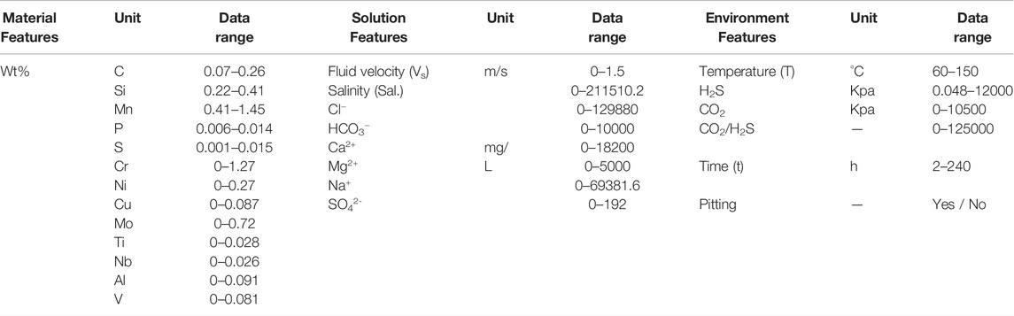
TABLE 1. List of features used in the machine learning models.

Features Selection

The purpose of feature selection is to simplify the feature set as much as possible and reduce the adverse effects caused by noise and redundant features while maintaining the description ability of feature set. This improves the accuracy, interpretability and operational efficiency of the model (Zhang et al., 2020).

In this section, feature variables are screened by combining feature importance calculation and Pearson correlation analysis. The former is based on the random forest model (RF model), which is composed of several simple classification and regression tree (CART) models. During the bootstrap sampling process, each CART model produces some data samples that are not selected for training. These data samples termed the out-of-bag (OOB) samples can be used to calculate feature importance (Zhi et al., 2019). For each CART, a disturbance is added to each input of OOB data and then calculate the variation amplitude of the predicted results. By comparing the amplitude of the variation, the importance of different inputs to the predicted target can be obtained. Finally, RF model obtains the average value of all CARTs’ results and calculating the importance of each feature is completed. Pearson correlation coefficient is a statistic used to reflect the linear correlation degree of two random feature variables (Waldmann, 2019). The coefficient obtained by estimating sample covariance and standard deviation ranges from −1 to 1. The greater the absolute value is, the stronger the correlation between feature variables is. For some machine learning models, the correlation between different feature variables has an important impact on the prediction results. Based on the above two methods, some redundant information can be removed from the original feature set, so as to achieve the purpose of feature reduction.

Feature combination is also a common method in feature engineering. Using the traditional theoretical calculation formula or model, several original features are combined into a new feature with practical significance. In this study, on the one hand, pitting resistance equivalent numbers (PREN) is calculated based on Chen et al. (2021a). PREN is a value calculated on the basis of the mass fraction of certain elements in the metal, and is usually used as a method to compare the pitting corrosion resistance of alloys. A common PREN expression is expressed as following:

$PREN=1\times wt\%Cr+3.3\times wt\%Mo+16\times wt\%N(1)$

On the other hand, the in-situ pH (pH_IS) of the solution is calculated using environmental and solution factors based on the electronic corrosion engineer (ECE) software (Jasim, 2019). Therefore, two feature parameters, PREN and pH_IS, are added by the method of the above feature combination.

In the aspect of feature creation, we explore a feature parameter that can contain the information of each element of steel and reflect the uniqueness of different steels. In this study, two different feature creation methods are proposed for each material. The feature creation method Ⅰ is defined by Eq. 2,

$Y_a=M_{a_1}{X}_{a_1}+M_{a_2}{X}_{a_2}+\dots +M_{an}{X}_{an}(2)$

where Y_a represents the element mass index of a material; M_a1,M_a2,_。。。M_an are the atomic mass of elements a₁,a₂,…a_n; X_a1,X_a2,_{。。。。。。}X_an represent the mass fractions of element a₁,a₂,……a_n. Method Ⅱ is defined by Eq. 3,

$\frac{Y_b}{Y_c}=\frac{M_{b_1}{X}_{b_1}+M_{b_2}{X}_{b_2}+\dots +M_{bn}{X}_{bn}}{M_{c_1}{X}_{c_1}+M_{c_2}{X}_{c_2}+\dots +M_{cn}{X}_{cn}}(3)$

where $\frac{Y_b}{Y_c}$ is defined as the mass index ratio of nonmetallic to metallic elements in a material; b₁,b₂…b_n represent the nonmetallic elements and c₁,c₂…c_n represent the metal elements. Two new features are generated.

Experimental Procedure

In this study, we first selected the appropriate dataset division ratio and machine learning classification algorithm through testing. Specifically, data of 40, 50, 60, 70, 80 and 90% were randomly selected from the original corrosion dataset after cleaning as the training set, and the remaining data as the test set. The training set was mainly used to optimize the classification model, and the test set was only used to identify the classification accuracy of the model. We prepared five machine learning classification models to be tested, including random forest classification model (RFC), support vector classification model with radial basis function kernel (SVC), gradient boosting decision tree classification model (GBC), naive bayes classification model (NB), and k-nearest neighbor model (KNN). Datasets of different proportions were input into different classification models for testing. During the training process, we used receiver operating characteristic (ROC) curve and area under curve (AUC) to evaluate the training effect of the model (Li et al., 2015). Each group of tests was repeated for 100 times, and the best-performing dataset division ratio and classification model were selected according to the average score.

Secondly, in terms of feature reduction, we conducted feature importance calculation and Pearson correlation analysis for all feature parameters (i.e., 13 material features, eight solution features, four environmental features and immersion time). noise and redundancy features were eliminated to form feature combination Ⅰ and based on this feature combination, pitting judgment model Ⅰ was established.

Thirdly, in the aspect of feature combination, two feature parameters (i.e., PREN and pH_IS) were added by using the traditional theoretical calculation model. For feature creation, we converted the information of each steel element into two feature parameters (i.e., Y_a and $\frac{Y_b}{Y_c}$). The four new feature parameters were combined with feature combination Ⅰ, and then the feature combination Ⅱ was formed after removing the features that contributed less to the target parameter, and the pitting judgment model Ⅱ was established. The performance of the two models was compared, and the improvement of the model’s generalization ability was demonstrated.

In the process of feature selection, model optimization and evaluation, F1 score was employed for the evaluation standard. In short, the F1 score is a measure of the classification problem and is a harmonized mean of precision and recall. Its value is approximately close to 1, indicating that the model has better performance (Lim and Chi 2021). For a binary classfication problem, a 2 × 2 confusion matrix is formed based on the forecast labels and actuality labels (as shown in Table 2), where the true positive (TP) refers to correct judgment of a positive sample (e.g., a case of pitting is correctly predicted) and a false positive (FP) means failure to judge a positive sample (e.g., a case of pitting is wrongly predicted). Similar definitions can be given to the false negative (FN) and true negative (TN). Further, precision, recall and F1 score can be respectively calculated by the following formulas:

$precision=\frac{TP}{\left(TP+FP\right)}(4)$

$recall=\frac{TP}{\left(TP+FN\right)}(5)$

$F1=2\frac{precision\times recall}{precision+recall}(6)$

TABLE 2

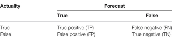
TABLE 2. Confusion matrix for binary classifier.

This research was based on python programming language, using Spyder3.3.6 software, and all machine learning algorithms involved in the research process were executed by the scikit-learn library. The main algorithm parameters are as follows: max_depth = 40 and n_estimators = 100 in RFC model; C = 170 and gamma = 0.5 in SVC model; max_depth = 10 and n_estimators = 100 in GBC model; k = 2 in KNN model, and all other parameters in the model are set to default values.

Results and Discussion

Selection of Dataset Division Ratio and Machine Learning Models

Based on the five classification models, the influence of different training set proportion on model performance was explored, and the results were shown in Figure 1. We randomly selected a specified proportion of test sets and repeated the test 100 times to evaluate the prediction performance of the model according to the average score. On the whole, as the proportion of the training set gradually increased, the prediction performance of the model gradually improved. This was because the amount of data in the training set was usually proportional to the effective information contained in it. Therefore, a larger proportion of the training set was highly likely to improve the comprehensive prediction performance of the model. However, when the proportion of training set increased to more than 80%, the F1 score of KNN model decreased significantly, while the F1 score of SVC model and NB model decreased slightly. This may be due to the overfitting of these algorithm, and thus, the generalization ability of the model is significantly reduced (Deng et al., 2015). Therefore, the division ratio of the training set selected in this study was 80%.

FIGURE 1

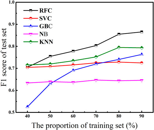
FIGURE 1. The pitting prediction performance of five different classification models in different proportions of datasets.

In the process of determining the partition ratio of training set, it was found that the RFC model had the best comprehensive performance. In order to further confirm the best model for predicting pitting, the ROC curve and AUC value of the five classification models were respectively drawn and calculated. The ROC curve, which defines false positive rate (FPR) as the X axis and true positive rate (TPR) as the Y axis, describes the relationship between TP and FP. The closer the ROC curve is to the upper left corner, the better the performance of the model (He et al., 2021). AUC is the area under the ROC curve and the larger the AUC, the higher the model performance. Figure 2 (A-E) were the ROC curves drawn based on the five different models (RFC model, SVC model, GBC model, KNN model and NB model). Among them, the method of five fold cross validation was used in the process and the blue line represented the average ROC curve. By comparison, the curve based on RFC model was closer to the upper left corner, which proved that this model had the best performance. In addition, the average AUC based on the RFC model was 0.84. Meanwhile, other classification models adopted the same method, and the calculated results of average AUC were shown in Figure 2F. The red lines represented the error range for 100 repetitions. As can be seen from the figure, RFC model had the best predictive performance, followed by NB model and GBCmodel, SVC model and KNN model had the lowest average AUC value. Combined with the above results, the RFC model was selected for subsequent studies.

FIGURE 2

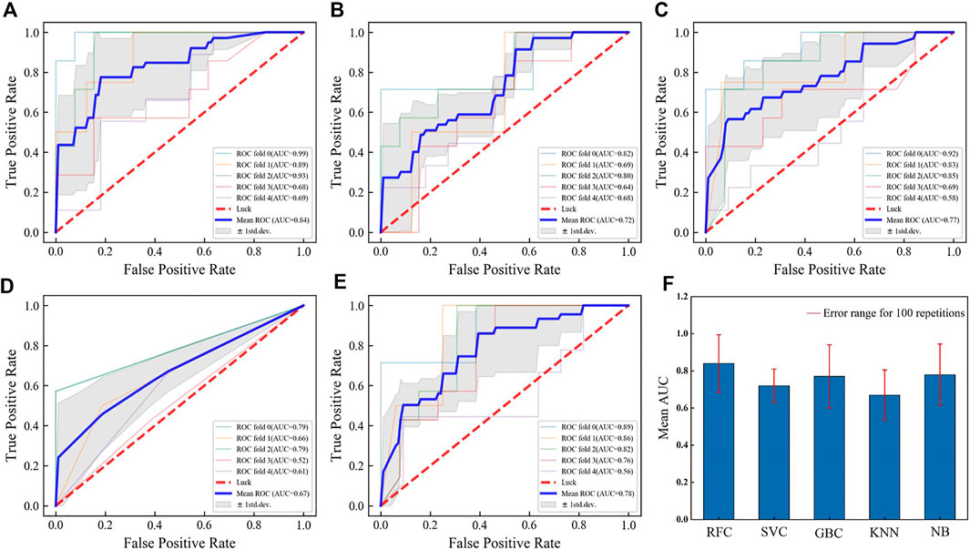
FIGURE 2. ROC curve and mean AUC obtained by cross-validation (A) When using the RFC model, (B) When using the SVC model, (C) When using the GBC model, (D) When using the KNN model, (E) When using the NB model, (F) When the five classification models are compared.

Effect of Feature Engineering on Model’s Performance

In the first step, the pearson correlation analysis method was used to reduce features. Specifically, input the original 13 material features, eight solution features, four environmental features and immersion time into the RF model, and the calculation results of feature importance were shown in Figure 3. To ensure the generalization ability of the model, we only selected the features with importance values above 0.02. (i.e., CO₂, T, CO₂/H₂S, H₂S of environmental features; Cl⁻, Sal., Na⁺, Ca²⁺, Mg²⁺, HCO₃⁻ of solution features; t). The combined importance of the selected 11 features exceeds 0.85, and they contain most of the information related to pitting.

FIGURE 3

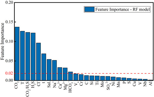
FIGURE 3. The feature importance sequence for 26 features based on RF model.

In terms of environmental features, CO₂ is usually present in corrosive solution in the form of a dissolved gas. HCO₃⁻ and H₂CO₃ is formed when CO₂ reacts with water and H⁺ produced in the ionization reactions of them can result in local acidification and pitting corrosion (Chen et al., 2021b). The solubility of H₂S in water is higher than that of CO₂. With the increase of the concentration of H₂S, H₂S decomposes into more H⁺ and HS⁻, which can change the local acidity of steel surface and promote the anodic dissolution process, thus affecting the pitting susceptibility of steel (Zhao et al., 2020). In addition, no matter in the corrosion process dominated by CO₂ or H₂S, the non-dense or non-uniform corrosion products formed on the surface of the steel can accelerate the development of pitting corrosion (Liu et al., 2017). Temperature is also a key factor affecting pitting, as many materials do not pitting below a certain temperature (critical pitting temperature), which has been demonstrated to exist (Mendibide and Duret-Thual 2018).

In terms of solution features, it is generally believed that Cl⁻ has a great influence on the pitting susceptibility of steel. In other words, the higher the content of Cl⁻, the looser the corrosion product scale formed on the steel surface and the more serious the cracking is. The Cl⁻ reaching the steel surface through the corrosion product scale can accelerate the local anode reaction, produce pitting pits and develop rapidly along the longitudinal direction (Liu et al., 2014b). Ca²⁺ and Mg²⁺ also have the ability to influence pitting susceptibility of steel significantly given that the presence of divalent salts can reduce CO₂ solubility (i.e., CaCO₃ in the case of Ca²⁺ presence and MgCO₃ in the case of Mg²⁺ presence) (Hua et al., 2018). Salinity refers to the total ion content in the solution, and the increase of its content can also change the solubility of CO₂ and H₂S, thus affecting the development of pitting corrosion (Han et al., 2011).

Then, we calculated the pearson correlation coefficient based on our dataset of solution features and environment features. As shown in Figure 4, the color (blue or red) indicates the direction of the relationship (positive or negative), and the intensity of the color indicates how strong the relationship is (white for completely unrelated and dark blue or red for perfectly correlated). Strong correlations occur between Sal., Na⁺, and Cl⁻, mainly because Cl⁻ and Na⁺ were usually very high in the solution being counted, and the salinity was almost composed of these two ions. Sufficient information could be obtained by selecting only one feature from a combination of features with strong correlation, and the importance of feature was usually proportional to the effective information contained in it (Wang et al., 2020). Thus, Cl⁻ was retained and Sal. and Na⁺ were discarded. Another feature combination with strong correlation was Ca²⁺ and Mg²⁺, which had a similar effect on the pitting susceptibility of steel. Ca²⁺ was also retained according to the above idea. The feature combination Ⅰ (i.e., CO₂, T, CO₂/H₂S, H₂S of environmental features; Cl⁻, Ca²⁺, HCO₃⁻ of solution features; t) was determined.

FIGURE 4

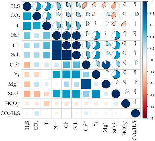
FIGURE 4. Pearson correlation matrix for 12 features.

Two feature parameters, PREN and pH_IS, were added by feature combination,and using feature creation method Ⅰ and Ⅱ, two new feature parameters were obtained, namely Y_a and $\frac{Y_b}{Y_c}$. The four newly generated feature parameters (i.e., PREN, pH_IS, Y_a, $\frac{Y_b}{Y_c}$) were combined with feature combination Ⅰ, and the feature importance was calculated and sorted (Figure 5). pH_IS and $\frac{Y_b}{Y_c}$ had great influence on the pitting judgment model, especially pH_IS, while the importance values of PREN and Y_a were relatively low. Pourbaix. (2009) have showen that the pitting potential of carbon steel becomes negative with the decrease of pH, which increases the susceptibility of pitting induction. To sum up, the two feature parameters (i.e., PREN and Y_a) were removed, and the feature combination Ⅱ including CO₂, T, CO₂/H₂S, Cl⁻, Ca²⁺, HCO₃⁻,t, pH_IS and $\frac{Y_b}{Y_c}$was selected as the input features of the pitting judgment model.

FIGURE 5

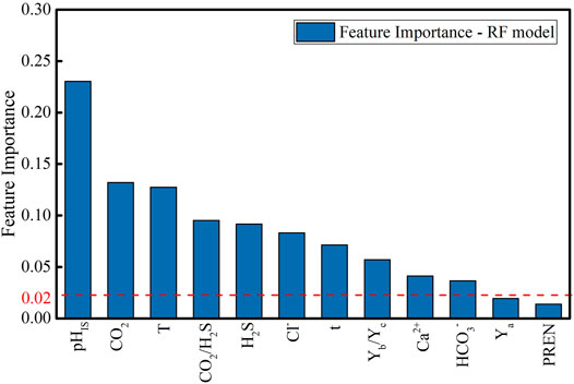
FIGURE 5. The feature importance sequence for 12 features based on RF model.

Based on above two different groups of input features (feature combination Ⅰ and Ⅱ), pitting judgment models Ⅰ and Ⅱ were individually established by RF model. Table 3 lists the predictive performance of each model. Each prediction process was repeated 100 times. By comparison, pitting judgment model Ⅱ with increased pH_IS and $\frac{Y_b}{Y_c}$ had a stronger performance, and the average F1 score for the training set and test set reached 0.996 and 0.987, respectively. As shown in Figure 5, the performance improvement of Model Ⅱ was mainly due to the two increased features, especially the pH_IS, which contributed greatly to judging whether pitting occurs. Therefore, we employed this model as the preferred model of pitting judgment.

TABLE 3

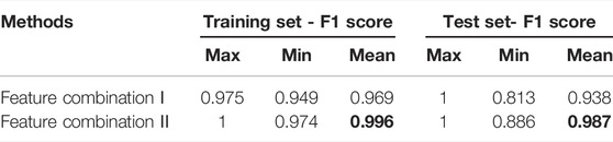
TABLE 3. The predictive accuracy of the pitting prediction model using the feature combination I and II, respectively.

As shown in Figure 3, the two most important feature parameters are CO₂ content and T for judging the occurrence of pitting. We tried to explore the law of pitting occurrence only through these two feature parameters. The relationship between T and CO₂ content with the occurrence of pitting is displayed in Figure 6. Surprisingly, both 3D scatter plot and the projection drawing of T and CO₂ content are disable to classify the occurrence of pitting. Pitting and non-pitting overlap each other, suggesting that the parameters of T and CO₂ content are not enough to distinguish the occurrence of pitting. Some other features also contribute to affect the pitting process. As we know, the development of pitting is an extremely complex process, and the influence of many factors must be considered comprehensively, which is exactly the advantage of machine learning model compared with traditional theoretical model.

FIGURE 6

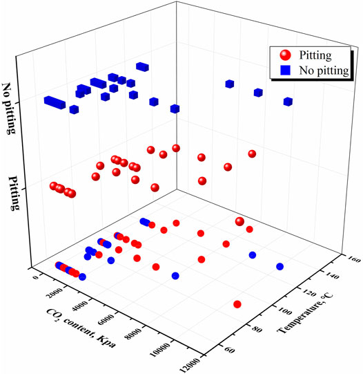
FIGURE 6. Influence of temperature and CO₂ content on the prediction of pitting.

Generalization Capabilities of Machine Learning Model

25 new rows of immersion test corrosion data (all parameters within the range) were collected (from our lab) as the validation set to verify the generalization ability of the model. The methods of feature reduction, combination, and creation were used to transform it into a feature set of the same type as feature combination Ⅱ, and then the pitting corrosion of each sample was predicted by the optimized model. As shown in Table 4, the pitting judgment model still shows a high prediction accuracy.

TABLE 4

TABLE 4. The results of model generalization performance.

Conclusion

In this study, we proposed a machine learning model based on experimental data to judge the occurrence of pitting for pipeline steel. Machine learning algorithm and feature engineering correlation method are used to analyze the relationship between the occurrence of pitting and input features such as material factors, solution factors and environmental factors. For this kind of material, CO₂, T, CO₂/H₂S, Cl⁻, Ca²⁺, HCO₃⁻,t, pH_IS and $\frac{Y_b}{Y_c}$ are considered to be the key factors to judge whether pitting happens or not. The generalization ability of the model is enhanced by replacing alloying element content with specific input parameters. Finally, the F1 scores of the optimized models were all greater than 0.97. Based on these results, machine learning method provides an effective means for processing high-dimensional and complex corrosion data, and can be a useful tool for further exploration of material corrosion problems.

Data Availability Statement

The original contributions presented in the study are included in the article/Supplementary Material, further inquiries can be directed to the corresponding author.

Author Contributions

ZQ, XL, and YL assembled the corrosion dataset and the feature set used in learning. ZW performed the machine learning. All authors analyzed the results and contributed in writing the manuscring.

Funding

This work was supported by National Key R&D Program of China (No. 2020YFB0704501).

Conflict of Interest

The authors declare that the research was conducted in the absence of any commercial or financial relationships that could be construed as a potential conflict of interest.

Publisher’s Note

All claims expressed in this article are solely those of the authors and do not necessarily represent those of their affiliated organizations, or those of the publisher, the editors and the reviewers. Any product that may be evaluated in this article, or claim that may be made by its manufacturer, is not guaranteed or endorsed by the publisher.

Supplementary Material

The Supplementary Material for this article can be found online at: https://www.frontiersin.org/articles/10.3389/fmats.2021.733813/full#supplementary-material

References

Balekelayi, N., and Tesfamariam, S. (2020). External Corrosion Pitting Depth Prediction Using Bayesian Spectral Analysis on Bare Oil and Gas Pipelines. Int. J. Press. Vessels Piping. 188 (12), 104224. doi:10.1016/j.ijpvp.2020.104224

CrossRef Full Text | Google Scholar

Bhandari, J., Khan, F., Abbassi, R., Garaniya, V., and Ojeda, R. (2015). Modelling of Pitting Corrosion in marine and Offshore Steel Structures - A Technical Review. J. Loss Prev. Process Industries. 37, 39–62. doi:10.1016/j.jlp.2015.06.008

CrossRef Full Text | Google Scholar

Bi, H., Li, Z., Hu, D., Toku-Gyamerah, I., and Cheng, Y. (2015). Cluster Analysis of Acoustic Emission Signals in Pitting Corrosion of Low Carbon Steel. Mat.-wiss. U. Werkstofftech. 46 (7), 736–746. doi:10.1002/mawe.201500347

CrossRef Full Text | Google Scholar

Chen, D., Dong, C., Ma, Y., Ji, Y., Gao, L., and Li, X. (2021a). Revealing the Inner Rules of PREN from Electronic Aspect by First-Principles Calculations. Corrosion Sci. 189, 109561. doi:10.1016/j.corsci.2021.109561

CrossRef Full Text | Google Scholar

Chen, X., Li, C. Y., Ming, N. M., and He, C. (2021b). Effects of Temperature on the Corrosion Behaviour of X70 Steel in CO₂-Containing Formation Water. J. Nat. Gas Sci. Eng. 88, 103815. doi:10.1016/j.jngse.2021.103815

CrossRef Full Text | Google Scholar

Choi, Y.-S., Shim, J.-J., and Kim, J.-G. (2005). Effects of Cr, Cu, Ni and Ca on the Corrosion Behavior of Low Carbon Steel in Synthetic Tap Water. J. Alloys Comp. 391, 162–169. doi:10.1016/j.jallcom.2004.07.081

CrossRef Full Text | Google Scholar

Deng, B.-C., Yun, Y.-H., Liang, Y.-Z., Cao, D.-S., Xu, Q.-S., Yi, L.-Z., et al. (2015). A New Strategy to Prevent Over-fitting in Partial Least Squares Models Based on Model Population Analysis. Analytica Chim. Acta. 880, 32–41. doi:10.1016/j.aca.2015.04.045

CrossRef Full Text | Google Scholar

Diao, Y., Yan, L., and Gao, K. (2021). Improvement of the Machine Learning-Based Corrosion Rate Prediction Model through the Optimization of Input Features. Mater. Des. 198, 109326. doi:10.1016/j.matdes.2020.109326

CrossRef Full Text | Google Scholar

Ghidini, T., and Dalle Donne, C. (2009). Fatigue Life Predictions Using Fracture Mechanics Methods. Eng. Fracture Mech. 76 (1), 134–148. doi:10.1016/j.engfracmech.2008.07.008

CrossRef Full Text | Google Scholar

Hadi Jasim, H. (2019). Evaluation the Effect of Velocity and Temperature on the Corrosion Rate of Crude Oil Pipeline in the Presence of CO2/H2S Dissolved Gases. Ijcpe 20 (2), 41–50. doi:10.31699/IJCPE.2019.2.6

CrossRef Full Text | Google Scholar

Han, J., Carey, J. W., and Zhang, J. (2011). Effect of Sodium Chloride on Corrosion of Mild Steel in CO2-saturated Brines. J. Appl. Electrochem. 41, 741–749. doi:10.1007/s10800-011-0290-3

CrossRef Full Text | Google Scholar

He, J., Li, J., Liu, C., Wang, C., Zhang, Y., Wen, C., et al. (2021). Machine Learning Identified Materials Descriptors for Ferroelectricity. Acta Materialia. 209, 116815. doi:10.1016/j.actamat.2021.116815

CrossRef Full Text | Google Scholar

Hu, J., Tian, Y., Teng, H., Yu, L., and Zheng, M. (2014). The Probabilistic Life Time Prediction Model of Oil Pipeline Due to Local Corrosion Crack. Theor. Appl. Fracture Mech. 70, 10–18. doi:10.1016/j.tafmec.2014.04.002

CrossRef Full Text | Google Scholar

Hua, Y., Shamsa, A., Barker, R., and Neville, A. (2018). Protectiveness, Morphology and Composition of Corrosion Products Formed on Carbon Steel in the Presence of Cl−, Ca2+ and Mg2+ in High Pressure CO2 Environments. Appl. Surf. Sci. 455, 667–682. doi:10.1016/j.apsusc.2018.05.140

CrossRef Full Text | Google Scholar

Jimenez-Come, M. J., Munoz, E., Garcia, R., Matres, V., Martin, M. L., Trujillo, F., et al. (2012). “Pitting Corrosion Detection of Austenitic Stainless Steel EN 1.4404 in MgCl2 Solutions Using a Machine Learning Approach,” in AIP Conference Proceedings. (American Institute of PhysicsAIP). doi:10.1063/1.4707652

CrossRef Full Text | Google Scholar

Kasai, N., Mori, S., Tamura, K., Sekine, K., Tsuchida, T., and Serizawa, Y. (2016). Predicting Maximum Depth of Corrosion Using Extreme Value Analysis and Bayesian Inference. Int. J. Press. Vessels Piping. 146, 129–134. doi:10.1016/j.ijpvp.2016.08.002

CrossRef Full Text | Google Scholar

Kolawole, S. K., Kolawole, F. O., Enegela, O. P., Adewoye, O. O., Soboyejo, A. B. O., and Soboyejo, W. O. (2016). Pitting Corrosion of a Low Carbon Steel in Corrosive Environments: Experiments and Models. Amr 1132, 349–365. doi:10.4028/www.scientific.net/AMR.1132.349

CrossRef Full Text | Google Scholar

Li, W.-f., Zhou, Y.-j., and Xue, Y. (2012). Corrosion Behavior of 110S Tube Steel in Environments of High H2S and CO2 Content. J. Iron Steel Res. Int. 19, 59–65. doi:10.1016/S1006-706X(13)60033-3

CrossRef Full Text | Google Scholar

Li, Y., Zhang, Y., Zhu, H., Yan, R., Liu, Y., Sun, L., et al. (2015). Recognition Algorithm of Acoustic Emission Signals Based on Conditional Random Field Model in Storage Tank Floor Inspection Using Inner Detector. Shock. Vibration. 2015, 1–9. doi:10.1155/2015/173470

CrossRef Full Text | Google Scholar

Lim, S., and Chi, S. (2021). Damage Prediction on Bridge Decks Considering Environmental Effects with the Application of Deep Neural Networks. KSCE J. Civ Eng. 25 (4), 371–385. doi:10.1007/s12205-020-5669-4

CrossRef Full Text | Google Scholar

Liu, M., Wang, J., Ke, W., and Han, E.-H. (2014a). Corrosion Behavior of X52 Anti-h2s Pipeline Steel Exposed to High H2S Concentration Solutions at 90 °C. J. Mater. Sci. Tech. 30 (05), 504–510. doi:10.1016/j.jmst.2013.10.018

CrossRef Full Text | Google Scholar

Liu, Q. Y., Mao, L. J., and Zhou, S. W. (2014b). Effects of Chloride Content on CO2 Corrosion of Carbon Steel in Simulated Oil and Gas Well Environments. Corrosion Sci. 84, 165–171. doi:10.1016/j.corsci.2014.03.025

CrossRef Full Text | Google Scholar

Liu, Z., Gao, X., Du, L., Li, J., Li, P., Yu, C., et al. (2017). Comparison of Corrosion Behaviour of Low-alloy Pipeline Steel Exposed to H2S/CO2-saturated Brine and Vapour-Saturated H2S/CO2 Environments. Electrochimica Acta 232, 528–541. doi:10.1016/j.electacta.2017.02.114

CrossRef Full Text | Google Scholar

Melchers, R. E. (2008). Extreme Value Statistics and Long-Term marine Pitting Corrosion of Steel. Probabilistic Eng. Mech. 23 (4), 482–488. doi:10.1016/j.probengmech.2007.09.003

CrossRef Full Text | Google Scholar

Mendibide, C., and Duret-Thual, C. (2018). Determination of the Critical Pitting Temperature of Corrosion Resistant Alloys in H2S Containing Environments. Corrosion Sci. 142, 56–65. doi:10.1016/j.corsci.2018.07.003

CrossRef Full Text | Google Scholar

M.Mohammad, H., J. Hammadi, N., and M. Lafta, R. (2013). Prediction of Pitting Corrosion Characteristics Using Artificial Neural Networks. Ijca 60 (4), 4–8. doi:10.5120/9678-4105

CrossRef Full Text | Google Scholar

Pourbaix, M. (1970). Significance of protection Potential in Pitting and Intergranular Corrosion. Corrosion 26, 431–438. doi:10.5006/0010-9312-26.10.431

CrossRef Full Text | Google Scholar

Santos, B. A. F., Serenario, M. E. D., Souza, R. C., Oliveira, J. R., Vaz, G. L., Gomes, J. A. C. P., et al. (2021). The Electrolyte Renewal Effect on the Corrosion Mechanisms of API X65 Carbon Steel under Sweet and Sour Environments. J. Pet. Sci. Eng. 199, 108347. doi:10.1016/j.petrol.2021.108347

CrossRef Full Text | Google Scholar

Soares, C. G., Garbatov, Y., Zayed, A., and Wang, G. (2009). Influence of Environmental Factors on Corrosion of Ship Structures in marine Atmosphere. Corrosion Sci. 51 (9), 2014–2026. doi:10.1016/j.corsci.2009.05.028

CrossRef Full Text | Google Scholar

Vajo, J. J., Wei, R., Phelps, A. C., Reiner, L., Herrera, G. A., Cervantes, O., et al. (2003). Application of Extreme Value Analysis to Crevice Corrosion. Corrosion Sci. 45 (3), 497–509. doi:10.1016/S0010-938X(02)00129-4

CrossRef Full Text | Google Scholar

Valor, A., Caleyo, F., Rivas, D., and Hallen, J. M. (2010). Stochastic Approach to Pitting-Corrosion-Extreme Modelling in Low-Carbon Steel. Corrosion Sci. 52 (3), 910–915. doi:10.1016/j.corsci.2009.11.011

CrossRef Full Text | Google Scholar

Waldmann, P. (2019). On the Use of the pearson Correlation Coefficient for Model Evaluation in Genome-wide Prediction. Front. Genet. 10. doi:10.3389/fgene.2019.00899

PubMed Abstract | CrossRef Full Text | Google Scholar

Wang, Y., Tian, Y., Kirk, T., Laris, O., Ross, J. H., Noebe, R. D., et al. (2020). Accelerated Design of Fe-Based Soft Magnetic Materials Using Machine Learning and Stochastic Optimization. Acta Materialia. 194, 144–155. doi:10.1016/j.actamat.2020.05.006

CrossRef Full Text | Google Scholar

Yin, Z. F., Zhao, W. Z., Bai, Z. Q., Feng, Y. R., and Zhou, W. J. (2007). Corrosion Behavior of SM 80SS Tube Steel in Stimulant Solution Containing H₂S and CO₂. Electrochimica Acta. 12, 039. doi:10.1016/j.electacta.2007.12.039

CrossRef Full Text | Google Scholar

Zhang, L., Chen, H., Tao, X., Cai, H., Liu, J., Ouyang, Y., et al. (2020). Machine Learning Reveals the Importance of the Formation Enthalpy and Atom-Size Difference in Forming Phases of High Entropy Alloys. Mater. Des. 193, 108835. doi:10.1016/j.matdes.2020.108835

CrossRef Full Text | Google Scholar

Zhao, X., Huang, W., Li, G., Feng, Y., and Zhang, J. (2020). Effect of CO2/H2S and Applied Stress on Corrosion Behavior of 15Cr Tubing in Oil Field Environment. Metals 10, 409. doi:10.3390/met10030409

CrossRef Full Text | Google Scholar

Zhi, Y., Fu, D., Zhang, D., Yang, T., and Li, X. (2019). Prediction and Knowledge Mining of Outdoor Atmospheric Corrosion Rates of Low alloy Steels Based on the Random Forests Approach. Metals 9, 383. doi:10.3390/met9030383

CrossRef Full Text | Google Scholar