Development of a Phase Field Tool Coupling With Thermodynamic Data for Microstructure Evolution Simulation of Alloys in Nuclear Reactors

We have developed a new phase field tool PHAFIS to automatically incorporate the thermodynamic data for both of WBM and KKS phase field simulations, which are widely used in the simulation of microstructure evolution of nuclear materials. Based on the generic C/C++ programming language, PHAFIS is capable of automatically parsing the standard TDB files, extracting the free energy and diffusion potential varying with the composition in an analytical way. Based on the two diffrerent TDB files of Fe-Cr binary system and the interpolated data, the phase morphologies during spinodal decomposition at 700 K and liquid-solid transition at high temperatures above 1800 K are reproduced and compared with each other by WBM and KKS model, respectively. Specifically, both of interface-controlled and diffusion-controlled phase transition mechanisms are successfully revealed for solidification through our KKS simulation, consistent with classic phase transition theories. It can be concluded that even slight differences in thermodynamic data will cause significant changes in the microstructure evolution. The integrity of our software tool will facilitate the coupling of phase field methods with thermodynamic data for other materials, paving a fundamental step for coupling more factors required in microstructure simulation.

Introduction

After the Fukushima nuclear accident, nuclear safety issues made the importance of the materials in the reactor particularly prominent, which is likely to be tackled in the concept of accident tolerant fuel (ATF) (Zinkle and Was, 2013). ATF is designed for developing new fuels to replace the existing UO2-Zr alloy, aiming at extending the operation time as much as possible under accident conditions and maintaining the same or better service performance under normal conditions. This may cause a conflict in this area between its urgency in application for reactors and the long duration for research and development (R&D) of nuclear materials that generally takes years or even decades. As a new paradigm of materials design, the Material Genome Initiative (MGI) is committed to reducing the development time and cost of materials discovery, optimization, and deployment, via computational materials methodology such as multi-scale simulations and big data methods. Therefore, it has been widely labelled as a potential solution for boosting nuclear materials industrialization, gaining enormous attention around the world since its launch in 2012 (Zinkle and Was, 2013). Among the hot topics of MGI, scientists and engineers are devoted into accomplishment of high-throughput and multi-scale simulations, which demand sophisticated coupling between different simulation algorithms from microscopic to macroscopic scales in efficient ways (Liu et al., 2004). However, there has not yet been a unified quantitative model to describe the complex microstructure evolution, which largely hinders the realization of multi-scale coupling for alloys in nuclear materials (Konings and Stoller, 2020).

The phase field model (PFM), which has been recognized as one of most powerful methodologies to simulate microstructural evolution at mesoscopic scale, such as solidification, martensitic transition, spinodal decomposition and grain growth etc. (Chen 2002; Emmerich 2008; Moelans et al., 2008; Ingo 2009; Qin and Bhadeshia, 2010). PFM can be used as a mesoscopic bridge to connect interstitial microscopic methods such as density functional theory (DFT), molecular dynamics (MD) (Liu et al., 2019) and macroscopic simulations, thus forming a typical multi-scale algorithm mode (Chen 2002; Moelans et al., 2008; Ingo 2009). PFM uses a series of free energy functionals and kinetic governing equations to continuously describe the evolution of order parameters, including phase fraction, grain orientation, chemical component and so on, without tracking the location of interfaces. For nuclear fuels and cladding materials, the phase field method has been applied not only to the simulation of fabrication processes (Guo et al., 2018), but also to the modeling of damage and defect evolution after irradiation (Li et al., 2017; Liang et al., 2018; Tonks et al., 2018; Cheniour et al., 2020), including bubble evolution, void formation and evolution, pore migration, interstitial loop growth and sink strength, segregation and precipitation. Although, at present, many of phase field simulations should be called qualitative or semi-quantitative, there has been an irreversible trend of gradually transitioning from qualitative PFMs to quantitative models aiming for system-specific predictive power (Tonks and Aagesen, 2019; Konings and Stoller, 2020). To this end, several major difficulties need to be overcome, including the inclusion of multiple physical mechanisms, accurate acquisition of model parameters, phase field programming and other computational efficiency issues (Tonks and Aagesen, 2019). At present, there are not many quantitative phase field simulations in the field of nuclear materials, which mainly focus on the microstructural evolution that do not involve complex phase transitions, such as grain growth in nuclear fuels (Ahmed et al., 2014; Mei et al., 2016; Cheniour et al., 2020) and radiation-induced segregation in Fe-Cr binary alloy (Piochaud et al., 2016), etc. The common feature of these simulations is that the input parameters of the phase fields are mainly low-scale parameters, such as lattice constants, elastic constants, interface energy and atomic mobility, which can be directly calculated by DFT or MD.

Different from low-scale parameters, however, thermodynamic data are more complex, such as free energy and diffusion potential of different phases in a certain ranges of temperature and chemical composition, which are particularly significant to quantitatively describe the driving force for phase transitions in binary and multiple phases. Generally, thermodynamic data are obtained and stored through sophisticated assessment by CALPHAD (CALculation of PHAse Diagrams) method, i.e., CALPHAD-type data. The CALPHAD method has been proved to provide accurate thermodynamic information consistent with phase diagrams for various materials including alloys, semiconductors, nuclear materials etc. (Lukas et al., 2007; Zhang et al., 2014). Therefore, phase field model combined with convincible CALPHAD-type data are expected to quantitatively simulate the thermodynamics for phase transitions in even multicomponent systems (Kitashima 2008; Nestler and Choudhury, 2011; Kattner 2016).

Nevertheless, the combination of the phase field model with thermodynamics data is not always straightforward and efficient up to now, although it has started since 2002 (Zhu et al., 2002; Kitashima 2008). In many cases, the usual way is to code the free energy formula manually into the phase field program (Zhu et al., 2002; Steinbach et al., 2007). Some others are trying to modify the phase field model to incorporate the CALPHAD models in a self-consistent way (Steinbach et al., 2007; Zhang et al., 2015). Zhang et al. (2015) proposed an interesting method to incorporate the sublattice models in the CALPHAD into phase field model with finite interface dissipation, which has been validated in some binary alloys. Basically, if a single material system and a small number of phases are involved in the phase field program, manual coupling may still work. However, it may bring difficulties in error handling and inefficiency for maintenance of the program, especially for large amount of thermodynamic data possibly involved in MGI. Therefore, it is urgent to adopt a way to automatically, accurately and effectively incorporate thermodynamic data into phase field models. Relying on the CALPHAD software, a phase field program can read the thermodynamic data processed by software or interact with the software dynamically (Qin and Wallach, 2003; Eiken et al., 2006), without considering the structure of the thermodynamic data. This cross-software coupling can be used to realize automatic coupling of thermodynamic data in an “indirect” way, in that the thermodynamic data is accessed by other software before entering the phase field program. Such a thermodynamic coupling method requires repeated calls to commercial software and interface programs with a license, reducing the overall phase field simulation efficiency, which is somewhat deviated from the original intentions of high efficiency and cost reduction proposed by MGI.

As for most phase field simulation, people are working on obtaining a phase field software that can automatically and self-consistently incorporate thermodynamic data. Generally, the variation of the free energy with composition and its first derivative (up to the second derivative) are necessary for the phase field models to construct the free energy functionals and to solve the governing equations. In other words, it is possible to implement a universal and reliable incorporation subroutine that can automatically import and analyze CALPHAD database files in the existing phase field programs, as long as the data files are sufficiently available and the format is standard. Fortunately, there are several open thermodynamic databases (van de Walle et al., 2018), in most of which the data are described in the “thermodynamic database” (TDB) format which can be seen as a de facto standard, first developed by Thermo-Calc company (Sundman et al., 1985; Andersson et al., 2002). TDB file stores all thermodynamic data in the form of ASCII code, which is highly readable by people and the majority of CALPHAD software. This facilitates the standardized implementation of phase field code to couple with CALPHAD data. With no help of CALPHAD software, unfortunately, TDB files are not readable for most phase field programs serving to different phase field models, although there are many available TDB files on the internet, like the National Information Management System (NIMS) database. Therefore, developing a program tool to effectively employ TDB files in the phase field program is of great significance for the establishment of quantitative phase field model, laying the foundation for its further application in multi-scale calculations. In this way, the required thermodynamic data can be easily coupled without changing the existing phase field program to the greatest extent, and a wider range of phase field workers can be attracted to participate in the multi-scale coupling work of MGI.

This article will demonstrate the development procedure of a phase field tool in C/C++ language which is capable of reading the standard TDB files written in TQ-language, extracting free energy parameters and construct phase field functionals, etc. To get a representative verification, we will focus on the binary alloy systems in the article. According to the classification of Tonk et al. (Tonks, et al., 2018), there are three basic phase field frameworks with most extensive application for nuclear materials, i.e., Wheeler-Boettinger-McFadden (WBM) and Kim-Kim-Suzuki (KKS), and grand potential (GP) phase field models (Wheeler, et al., 1992; Wheeler, et al., 1993; Kim, et al., 1999). The WBM and KKS models lose no accuracy of the thermodynamic data and will be chosen to characterize the effectiveness of our thermodynamic coupling. As a main component of Fe-Cr-Al alloy, a very promising ATF cladding materials candidate, as well as other ferrite stainless steels, the Fe-Cr system with body-centered cubic (BCC) structure is taken as an example to demonstrate the applicability of our program in nuclear materials. The spinodal decomposition and liquid-solid transition of the Fe-Cr binary system are modeled to show the reliability of our phase field program. In addition, two versions of TDB files from open databases and literatures are used to show the difference in the microstructural morphologies caused by different thermodynamic assessments.

Models

In this section, we will briefly introduce the binary WBM and KKS phase field models, and the sublattice solution model as one of the most widely used CALPHAD models for solid-solution alloys in the frame of compound energy formalism (CEF) (Hillert 2001).

Binary WBM and KKS Phase Field Models

In fact, for a binary system, the WBM model can be regarded as a special case of KKS model. Therefore, we will introduce the models based on the architecture of the KKS model. We aim to simulate the solidification of the Fe-Cr binary alloy system, i.e., liquid to BCC structural transition, and the spinodal decomposition of Fe-Cr solid. For solidification simulation, two order parameters are included, that is, phase fraction of solid phase $\varphi \left(\overrightarrow{r},t\right)$ , ($\overrightarrow{r}$ denotes the position vector and t is time), and solute concentration (e.g. mole fraction of Cr in Fe-Cr) $c\left(\overrightarrow{r},t\right)$ in our phase field models. $\varphi \left(\overrightarrow{r},t\right)$ can be defined as a normalized total molar density, with equilibrium values 0 and 1 referring to the liquid and solid phases, respectively.

According to the gradient thermodynamics (Cahn and Hilliard, 1958), the total free energy F of a liquid–solid system can be written as

$F=\frac{1}{V_m}{\displaystyle {\int }_V\left[f\left(c,\varphi ,T\right)+\frac{\alpha }{2}|\nabla c{|}^2+\frac{\beta }{2}|\nabla \varphi {|}^2\right]}dV(1)$

where α and β are the gradient energy coefficients (Chen 2002). V is the total volume of the liquid–solid system, V_m is the molar volume of the system. In the KKS model,

$f\left(c,\varphi ,T\right)=f\left(c_S,c_L,\varphi ,T\right)=h\left(\varphi \right)G^S\left(c_S,T\right)+\left(1-h\left(\varphi \right)\right)G^L\left(c_L,T\right)+wg\left(\varphi \right)(2)$

where f denotes the bulk free energy density of the whole system. G^s and G^L are the free energy densities of solid and liquid as a function of temperature and solute concentration, respectively. h(ϕ) = ϕ³(6ϕ²−15ϕ + 10) is the commonly used interpolation function to make h(0) = 0 and h(1) = 1. g(ϕ) = ϕ²(1−ϕ)² is a double-well potential with the height of w. For the KKS model, concentration c can be seen as a synthetic term of c_s and c_L, written as

$c=h\left(\varphi \right)c_S+\left[1-h\left(\varphi \right)\right]c_L(3)$

where c_s and c_L are solute concentrations of solid and liquid phases respectively in the interfacial region, while satisfying the condition of equal diffusion potentials η, i.e.,

$\eta =\frac{\partial G^S\left(c_S\left(x,t\right)\right)}{\partial c_S}=\frac{\partial G^L\left(c_L\left(x,t\right)\right)}{\partial c_L}.(4)$

The governing equations for c and ϕ are following as

$\frac{\partial c}{\partial t}=\nabla \cdot \left[M_c\frac{\delta F}{\delta c}\right](5)$

$\frac{\partial \varphi }{\partial t}=-L_{\varphi }\frac{\delta F}{\delta \varphi }(6)$

where M_c and L_ϕ represent the mobility of c and ϕ, respectively. The specific parameterization of M_c and L_ϕ will be shown in the following sections. For the KKS model, Eqs. (5, 6) can be equivalently transformed to be

$\frac{\partial c}{\partial t}=\nabla \cdot \left(D\left(\varphi \right)\nabla c\right)+\nabla \cdot \left[D\left(\varphi \right)h^{\prime }\left(\varphi \right)\left(c_L-c_S\right)\nabla \varphi \right](7)$

$\frac{\partial \varphi }{\partial t}=L_{\varphi }\left[\nabla \cdot {\epsilon }^2\nabla \varphi +h^{\prime }]\left(\varphi \right)\left[P_{c_L}-P_{c_S}\right]\right]-w{g}^{\prime }\left(\varphi \right),(8)$

where P_ci = fⁱ(c_i)−c_iμ,{i = L(liquid), S(solid)} and D(ϕ) = h(ϕ)D_s + (1−h(ϕ))D_L is the solute diffusivity as a function of ϕ (Li et al., 2007). It should be noted that the KKS model is reduced to the WBM model when c = c_s = c_L is adopted. If spinodal decomposition is modeled in a single phase, the WBM and KKS models can be considered as the same one that contains only one order parameter $c(\overrightarrow{r},t)$. Additionally, the interfacial energy between liquid and solid can be estimated by

$\sigma =\sqrt{{\beta }^{\ast }w/18}(9)$

and the interfacial width by

$d=2.2\sqrt{2\beta /w}(10)$

consistent with Kim et al., (1999). Therefore, the values of β and w can be determined uniquely by given d and σ. Particularly, interfacial energy σ can be anisotropic and dependent on the interfacial morphology, i.e., $\sigma \left(\overrightarrow{n}\right)$ , where $\overrightarrow{n}=(n_x,n_y,n_z)=(\partial \varphi /\partial x,\partial \varphi /\partial y,\partial \varphi /\partial z)$ denotes the normal vector of an interface. If the cubic anisotropic of the interface is assumed, $\sigma \left(\overrightarrow{n}\right)$ can be represented with the average σ₀ and anisotropy parameter δ (<0.0625) as

$\sigma \left(\overrightarrow{n}\right)={\sigma }_0\left(1-3\delta \right)\left[1+\frac{4\delta }{1-3\delta }\left(n_x^4+n_y^4+n_z^4\right)\right](11)$

Apart from kinetic parameters, for the WBM model, the bulk free energy of the phases and their first derivatives with respect to solute concentration should be derived from thermodynamic data, on the basis of Eq. (1). For the KKS model, additional information is needed, i.e., solution of Eq. (4). Therefore, the bulk free energy is the key to incorporate thermodynamic data into the phase field models.

Sublattice Solution Model

Sublattice solution model (SSM) with the Redlich–Kister formula (Redlich and Kister, 1948) in the frame of CEF is one of the most popular models for approximating the Gibbs free energy of crystalline solids (Lukas et al., 2007). SSM uses the concept of constituent fractions (denoted as y) to represent how the atoms may occupy different types of sublattices with different coordination numbers, bond lengths, etc. Because of its advantages in the description of disordered/ordered phases, SSM has attracted much attention as a fundamental assessment model and is also supported by the TDB format. The total Gibbs energy of a phase θ in alloy can be generally expressed as

$G_m^{\theta }\left(\mathbf{y}\right)=G^{ref}\left(\mathbf{y}\right)+\Delta G_{mix}^{ideal}\left(\mathbf{y}\right)+G^{exc}\left(\mathbf{y}\right)+G^{mag}\left(\mathbf{y}\right)+\mathrm{...}(12)$

where y represents the constituent fraction vector, G^ref the free energy on the reference surface, ΔG^id_mix the ideal mixing entropy contribution, G^exc the excess free energy by using Redlich–Kister formula (Redlich and Kister, 1948), and G^mag expresses the magnetic energy of alloy (Hillert and Jarl, 1978). In this article, we will focus on the above four energies, although other contributions (such as disorder/order transition) can also be taken into account in a similar way. More details with respect to the parameters in the model can be found in the reference (Lukas et al., 2007).

PHAFIS Program

PHAFIS (PHase diAgram driven phase FIeld simulation Software) is our newly developed software module coded in C/C++, to couple thermodynamic data for phase field simulation, which can be seen in Figure 1. It is capable of parsing the standard TDB file format, extracting the mathematical expression of all phases, calculating accurately the free energy and the 1^st derivative with respect to solute concentration at a given temperature, and interpolating the free energy to accelerate phase field simulation. PHAFIS and our existing solving modules for phase field models can be seamlessly connected, laying a foundation for accurate calculation of true material systems.

FIGURE 1

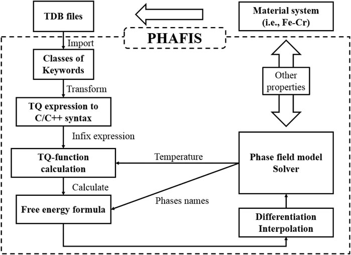
FIGURE 1. TDB incorporation procedure. Once a TDB file of a material system is given, it will be parsed and converted into C/C++-compliant grammars. After solving the infix expression, the free energy expression at constant temperature can be obtained, which will be used by phase field model solver by differentiation and interpolation.

Incorporation Procedure of TDB Files

In this section, we will start with the basic syntax and structure of standard TDB format, then establish the data structure for the free energy of a phase according to the sublattice solution model, and finally incorporate the thermodynamic data into the phase-field models. The entire coupling process is executed by the generic C/C++ language program, keeping its compatibility and portability to the maximum.

Parsing the Standard TDB Format

Although the TDB format was first built by Thermo-Calc, it has now become one of the most popular thermodynamic data storage format standards. The standard TDB format is ASCII-encoded and contains multiple keywords to describe the core thermodynamic information for various phases composed of certain elements, including its definition, constituents, and thermodynamic model parameters, etc. The TDB standard file is highly readable, which is not only convenient for readers, but also conducive to the effective identification of computers.

Specifically, there are at least six keywords that are essential for building the free energy of a phase, including “ELEMENT”, “FUNCTION”, “PHASE”, “TYPE_DEFINITION”, “CONSTITUENT”, “PARAMETER”. The keyword "ELEMENT" gives all the basic elements needed to make up all the phases in a TDB file. "FUNCTION" contains mathematical expressions in terms of temperature and pressure required by the thermodynamic model, including the standard element reference (SER) (Dinsdale, 1991) and other customized functions. As for “PHASE”, it defines a thermodynamic phase with some sublattices, e.g. liquid, BCC_A2 and FCC_A1. There are constituents in the sublattices, which are further interpreted in the keyword “CONSTITUENT”. In some cases, the definition of a phase can be modified to possess more properties, such as adding magnetic contributions for a ferromagnetic phase, which can be accomplished in the keyword “TYPE_DEFINITION”. The last, but not the least important, “PARAMETER” represents all the parameters essential to calculate the free energy of a phase according to the thermodynamic model, combining with all other keywords. With different expressions, these keywords complementarily describe the required thermodynamic information of various phases. Our C/C++ program has built the corresponding C++ classes for the above six keywords conforming to the relevant syntax.

As far as the syntax of standard TDB format is referred to, some points that alter the free energy calculations need to be noted. Firstly, the main syntax is based on the TQ-language, analogy to Fortran. The Fortran-like mathematical expression, for example, logarithmic function “LN ()”, power function operator “()**()” , exponential function “EXP ()”, and so on, will be converted to their counterparts in C/C++ in our program. Another feature of TDB format is that there are some special characters or symbols owning their specific meanings, which ought to be identified in the program. Specifically, they include annotation character “$”, terminator “!”, continuation character “Y” and discontinuation “N” in TQ functions; sublattice separator “:”, constituent separator "," and parameter separator ";" in the definition of parameters in a thermodynamic model, as shown in Table 1. Everything related to the calculation of free energy in the TDB file will be parsed and converted according to the syntax of C/C++ for later handling in our program.

TABLE 1

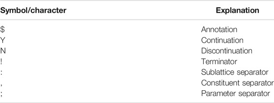
TABLE 1. Explanation of some special symbols.

Calculating TQ Expressions

Generally, the TQ expressions in the keywords of “FUNCTION” and “PARAMETER” are mathematical functions of temperature T and pressure P. Considering that most TDB files are assessed under the atmospheric pressure, the dependence of the expressions on P is ignored for simplicity. Moreover, it is common to conduct phase field simulation at constant temperature, for instance, isothermal solidification and annealing. Therefore, after the TQ expressions are converted into C/C++, they will be numerically calculated based on the temperature of the phase field simulation by an infix expression calculator in our program. Thus, the numerical values of all necessary parameters for all phases at any temperature are obtained immediately and stored into the memory of computers. In other words, one can get a parameter library required for calculating free energy of any phase by reading the TDB file for only one time.

It seems to be redundant to store the data of the non-target phases for a common phase field simulation of some target ones. In fact, such redundant storage might be beneficial to multi-scale coupled and high-throughput calculations in MGI for nuclear materials. Then, a unified parameter library can not only improve the operation efficiency but also reduce the probability of unexpected errors due to excessive interaction with the original TDB files.

Constructing Free Energy Expressions

At this step, the expressions of free energy (as Eq. (12)) are built with its first derivative based on the sublattice solution model by our program. Since the free energy in Eq. (12) are all simple mathematical functions of constituent fractions y, our program can automatically construct the analytical expressions of free energy as well as its first and second derivatives with respect to y given a phase name. Higher-order derivatives can also be obtained analytically, although this is not necessary for the WBM and KKS models. Notably, the constructed expressions of free energy and derivatives are functions of constituent fractions y. As long as the constituent fractions are given, the corresponding numerical values of free energy and derivatives can be obtained immediately through our internal calculator. Alternatively, numerical differentiation can be performed to gain the expressions of the derivatives based on the results of free energy.

Incorporating Free Energy Data Into Phase Field Models

In order to facilitate the incorporation of free energy data into the phase field models, one of the most efficient ways is to store the data in a discrete manner and use it after interpolation. First, a set of discrete data that the free energy varies with temperature and constituents can be calculated for a certain range of constituent fraction (e.g. 0 to 1) with a certain interval step (e.g. 0.01). Then, the free energy for any constituent fraction can be obtained readily by interpolating the discrete data through interpolation methods. In this program, for simplicity, the linear interpolation methods are used. So far, the WBM phase field model can be initiated with the interpolation of free energy and its first derivative (called diffusion potential here) (Plapp 2011), while these are insufficient for the KKS model since it has two more equations to be solved, i.e., Eqs. (3,4), for c_s and c_L. In order to speed up the computational efficiency of phase field simulation, the paired solution (c_s,c_L) obtained under different values of (c,ϕ) will be made into a lookup table. Considering that both of c and ϕ are between 0 and 1, they are respectively discretized into N_c,ϕ points with a step size, like 0.01. Then, solving for Eqs. (3,4) produce a solution (c_s,c_L) given with (c_i,ϕ_j),i,j∈[1,N_c,ϕ], constructing a high-dimensional loopkup table. With this mapping relationship (c,ϕ)–>(c_s,c_L) , (c_s,c_L) can be calculated after interpolation with arbitrary combination of c and ϕ.

Verification in Fe-Cr Binary System

To verify the reliability of our program, the Fe-Cr binary alloy is chosen as the object system with Cr as the solute atom. Since the thermodynamic data of Fe-Cr has been being updated and developed, two versions of Fe-Cr TDB files, i.e., one copied from NIMS database (Byeong-Joo 1993) (named as TDB1), and one assessed newly in 2018 (Jacob et al., 2018) (named as TDB2), are included for the verification. Specifically, the liquid and disordered solid (BCC_A2) phases are selected under investigation. In this case, solidification of the liquid phase to BCC occurs at high temperatures, and spinodal decomposition in the BCC phase happens at intermediate temperatures, expected to be described properly by the KKS and WBM models.

Free Energy and Diffusion Potential

Before the phase field simulation, the free energy and diffusion potential varying with Cr concentration (denoted as c(Cr)) are obtained. Particularly, in order to realize the automatic configuration of TDB reading and interpolation, a customized configuration file has been designed to define the indispensable parameters, including a TDB file path, a phase name with basic sublattice information, the constituent ranges and intervals for interpolation, etc. For verification, the free energy of liquid and BCC_A2 phases at 700 and 1800 K are calculated by our program and shown in Figures 2A,B, respectively. It should be pointed out that we have calculated the same free energy with OpenCalphad (OC, version 5.004) (Sundman et al., 2015), a free thermodynamic software, and obtained exactly the same results, which will not be shown in the figures again. At 700 K, the free energy of solid phase is significantly lower than that of liquid one, and shows double potential wells at the concentration around 0.1 or 0.8, indicating that spinodal decomposition is expected to occur at the some conditions, which will be shown in the next section. When the temperature reaches 1800 K, the free energies of the solid phase and the liquid phase are relatively close, and there should be a stable region of the solid phase if the solute concentration is higher than 0.4, leading to the occurrence of solidification for both TDB files. Mostly, the free energy of TDB2 is slightly lower than that of TBD1, whereas the effect of this difference on the liquid-solid phase transition is still uncertain. As for the diffusion potential η, two methods are used to calibrate the derivative of free energy, namely the analytical solution η_a and the two-point difference numerical solution η_b. Figure 2C shows the comparison between the two solutions for BCC_A2 phase at 700 K for TDB2 as an representative example, with the relative error ε = |1−η_b/η_a| × 100%. ε is basically below 10⁻³ for most of the curve, except for η close to zero as well as concentration approaching 0 or 1, which can be attributed to the amplifying errors when η_a→0 and using the finite difference stencil near the endpoints. For example, the errors can be mitigated by reducing the interval of interpolation data, but this will deteriorate the numerical efficiency. Therefore, special care needs to be taken when solving the derivatives of free energy numerically, otherwise more serious errors will emerge when seeking higher-order derivatives.

FIGURE 2

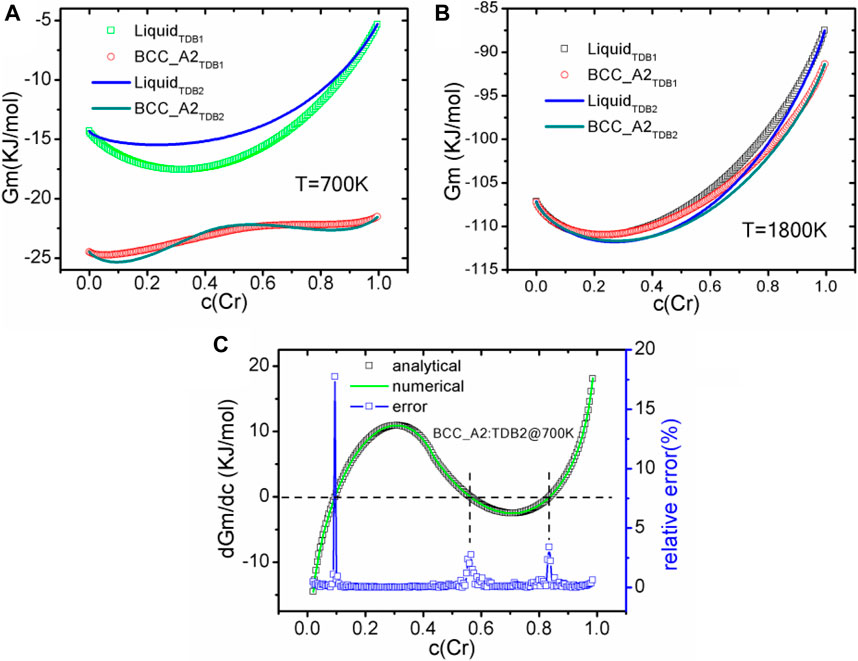
FIGURE 2. (color online) The variation curves of liquid phase and BCC_A2 with Cr composition calculated from different TDB files, (A) 700 K, (B) 1800 K. (C) Comparison between diffusion potentials at 700 K calculated analytically and numerically, and the corresponding relative error (in%) of TDB2.

Spinodal Decomposition

Here, the WBM model is employed to simulate the spinodal decomposition (SD) phenomenon of solid phase BCC_A2 at constant temperature . Only one order parameter $c(\overrightarrow{r},t)$ defined as the mole fraction of Cr, is enough to describe the morphology evolution in the binary alloy by solving Eq. (1) and Eq. (5). TDB1 and TDB2, respectively, are used to perform phase field simulations, while keeping most of the model parameters unchanged. Firstly, T^SD = 700K , and the concentration field $c(\overrightarrow{r},t=0)=c_0+\xi \left(\overrightarrow{r}\right)$ , where c₀ = 0.4 is the average concentration of the system, ξ denotes the Gaussian white noise term with amplitude of 10⁻³. Secondly, the free energies and diffusion potentials from the two TDB files are compared as functions of Cr concentration c(Cr) at T^SD, as shown in Figure 3. Both curves have two valleys and coincide at both ends, indicating that spinodal decomposition is possible to occur from a thermodynamic point of view. However, the curve of TDB2 has lower free energies at the valleys, inferring higher stability of the phases through spinodal decomposition than that of TDB1. In addition, the concentrations corresponding to the two valleys of TDB1 are closer to 0 and 1 than TDB2. Also, the diffusion potential near c₀ for TDB2 is higher than TDB1, indicating that the nucleation of spinodal decomposition for TDB2 may occur earlier.

FIGURE 3

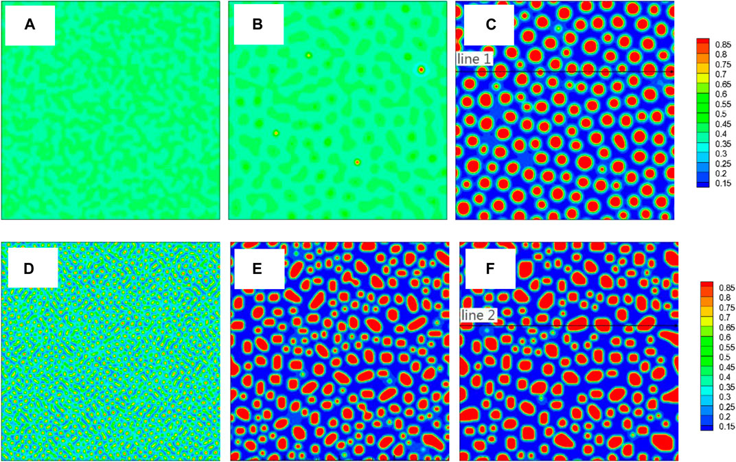
FIGURE 3. (color online) Images of concentration field corresponding to three different moments from the two TDB files, TDB1: (A)1 × 10³Δt, (B)5 × 10⁴Δt, (C) 1 × 10⁵Δt, TDB2: (D)1 × 10³Δt, (E)5 × 10⁴Δt, (F)1 × 10⁵Δt. The concentration along the two black lines in (C) and (F) will be shown in Figure 4.

In addition to the free energy of the solid phase, there are several model parameters to be determined, including molar volume V_m, gradient coefficient α, and concentration mobility M_c. First, we start with estimating the value of V_m. Since the thermal expansion coefficient of solid Fe-Cr alloys is very small, generally on the order of 10⁻⁵K⁻¹, the crystal structure can be assumed to be perfectly BCC. Thus, V_m can be estimated through the lattice constant a₀ varying with the concentration c, which is assumed to follow the Vegard’s law (Denton and Ashcroft, 1991), i.e., a₀ ≈ ca_cr + (1−c)a_Fe with the lattice constants a_Fe = 0.28670 nm and a_cr = 0.28844 nm (Gale and Totemeier, 2004). Next, value of α is estimated as (Li et al., 2009)

$\alpha =k_{\alpha }{\Psi }_{FeCr}(13)$

where k_α = d²₀/6V_m is a scaling factor, d₀ is the interatomic distance and can be set as the nearest neighbor atomic spacing of Fe-Cr alloy, and Ψ_FeCr denotes the interaction strength between the constituents Fe and Cr and can be derived from the thermodynamic data (Li et al., 2009). According the two incorporated TDB files, specifically,

${\Psi }_{FeCr}^{\left(TDB1\right)}=20500-9.68\ast T(14)$

in the TDB1, and

$\begin{array}{l}{\Psi }_{FeCr}^{\left(TDB2\right)}=24600-14.98\ast T+\left(500-1.5\ast T\right)\ast \left(2c-1\right)\\ +\left(-14000+9.15\ast T\right)\ast {\left(2c-1\right)}^2\end{array}(15)$

in TDB2. The last parameter is chemical mobility M_c which can be expressed as

$M_c=\left(c{M}_{Cr}+\left(1-c\right)M_{Fe}\right)V_{m}c\left(1-c\right)(16)$

where M_i = D_i/RT,i = {Fe,Cr} denotes the mobility of constituent i (Shewmon, 2016), R is the gas constant and T the absolute temperature, and

$D_i=D_{i,0}\exp \left(-\frac{\Delta H_i}{RT}\right),(17)$

represents the self-diffusivity of species i, with the pre-exponential factor D_i,0 and the activation enthalpy ΔH_i (Mehrer, 2007). For BCC iron and chromium, their dominant diffusion mechanisms are regarded as vacancy diffusion, which will be affected by changes in their magnetic states, especially for iron. In fact, there are two sets of diffusion parameters (D₀ and ΔH) near the Curie temperature T^Fe_c for iron, for both the paramagnetic and ferromagnetic states. It is assumed here that the choice of iron diffusion parameters depends on the Curie temperature (denoted as T^FeCr_Curie) of the binary alloy system. In other words, the diffusion parameters for the ferromagnetic state are selected below T^FeCr_Curie, and the other one above. Actually, the addition of Cr will lower T^FeCr_Curie( Braun and Feller-Kniepmeier, 1985), which may obscure the choice of diffusion parameters for iron. Based on the contents of TDB1 and TDB2, T^FeCr_Curie are estimated as 871 and 751 K, respectively, if the average concentration c₀ = 0.4 is used on the basis of Redlich–Kister (RK) polynomial (Redlich and Kister, 1948; Lukas et al., 2007). Now, the diffusion parameters for the ferromagnetic iron can be unambiguously used at T^SD = 700K . However, due to the difficulty in quantitatively obtaining extremely low diffusion coefficients at low temperatures, the diffusion enthalpies of Fe and Cr remain controversial (Peterson et al., 1969; Lübbehusen and Mehrer, 1990; Seeger, 1998; Shewmon 2016). Here, we choose to use the experimental data reviewed recently by Neumann and Tuijn (Neumann and Tuijn, 2011). By fitting the credible data through Eq. (17), the diffusion parameters we obtained are as follows, ΔH_Fe ≈ 332 kJ/mol with D_Fe,0 ≈ 1.53 m²/s for the ferromagnetic iron, and ΔH_Cr ≈ 439 kJ/mol with D_Cr,0 ≈ 0.11 m²/s . As a reference, the activation enthalpy is approximately 260 kJ/mol in the paramagnetic α-Fe (Neumann and Tuijn, 2011).

In our simulation, M_c changes with the concentration field, while V_m and α are assumed to be constant and evaluated by fixing c = c₀ for simplicity, resulting in α₁ = 2.26 × 10⁻¹¹J/m and α₂ = 2.42 × 10⁻¹¹J/m for TDB1 and TDB2 respectively, V_m = 7.15 × 10⁻⁶m³/mol. Except for the gradient coefficients (α₁ and α₂) that are directly derived from the TDB files, all the other parameters for the simulation remain the same. The dimensionless parameters are calculated through the reference quantities including, the length scale l^ref = 0.1 nm, the free energy density E^ref = 1 × 10⁹J/m³, and the time scale t^ref = 1 × 10⁵s. Our phase field program runs for a 2D block of 200Δx*200Δx with the uniform dimensionless grid size Δx = 1.0 and periodic boundary conditions in all dimensions. The dimensionless time step is Δt = 0.005.

Figure 3 shows the images of concentration fields from the two TDB files (upper row (a-c) for TDB1 and lower row (d-f) for TDB2) at different times as 1 × 10³, 5 × 10⁴ and 1 × 10⁵ Δt, corresponding to the three columns from left to right, respectively. A large number of nucleation processes occur in the early period of evolution for TDB2, while the nucleation is in incubation for TDB1, as displayed in Figures 3A,D. In fact, the nucleation process does not begin until the time close to 5 × 10⁴Δt, meanwhile, the particles in TDB2 have been coarsening, as exhibited in Figures 3B,E. Interestingly, after a longer time, there are similarities with respect to the particle distributions in Figures 3C,F. In fact, after long-term evolution, the concentrations in Cr-rich and Fe-rich regions can be approximately regarded as in near-equilibrium state, which are expected to be different according to the free energy curves in Figure 2A. To compare the near-equilibrium concentrations, the data along the line1 in Figure 3C and line2 in Figure 3F are extracted and plotted in Figure 4A. It can be clearly seen that the peak value of TDB1 is higher than that of TDB2 with the valley values close to each other. After global statistics, the peak and valley values of TDB1 are approximately 0.93 and 0.12, respectively, and those of TDB2 as 0.91 and 0.13. Then, the volume fraction of Cr-rich phase can be estimated as 34.57 and 34.62% for TDB1 and TDB2, which are nearly the same.

FIGURE 4

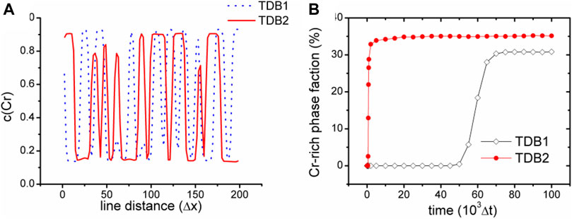
FIGURE 4. (color online) (A) Cr concentration along the two black lines highlighted in Figures 3C,F(B) variation of phase fraction with Cr concentration higher than 0.5 with time.

To compare the evolutionary dynamics in a more quantitative way, a phase fraction χ of Cr-rich phase is defined as the volume fraction with Cr concentration greater than 0.5 in the whole simulation block, whose evolution with time is shown in Figure 4B. We can see that χ₂ of TDB2 increases rapidly close to 35% in the early stage of evolution, and then approached a slowly rising plateau, which is quantitatively consistent with the theoretical value. For TDB1, χ₁ quickly rises to about 30% after a longer period of incubation. The dynamics of TDB1 is significantly slower than that of TDB2, mainly because of the lower diffusion potential around 0.3 as well as smaller gradient coefficient α₁, which contributes a low driving force and a longer period of incubation for the phase transition. As one of the most classic applications of phase field model, the simulation of SD exhibits that different TDB files may cause obvious differences in the kinetic process, while the final equilibrium morphologies are still similar with each other. Therefore, in order to quantitatively simulate the dynamics of SD, it is necessary to carefully select the appropriate thermodynamic data.

Liquid-Solid Transition

The second example to be verified is a liquid-solid (LS) transition process of the BCC_A2 phase in an undercooled melt with average concentration c₀ = 0.5 at T^LS = 1800 K via the KKS model. Specifically, Eq. (6) is used to give the evolution of the phase field $\varphi (\overrightarrow{r},t)$ , and concentration field $c(\overrightarrow{r},t)$ will be solved by Eq. (7) combined with Eqs (3,4). To speed up the numerical efficiency of the KKS model under the condition of equal diffusion potentials, i.e., Eq. (4), the discrete solutions are first calculated and tabulated for interpolation.

As for the parameters to be determined in the KKS model, the same molar volume V_m = 7.15 m³/mol will be used as that in the previous section. Besides, β and w in the free energy functional can be solved through Eqs. (9,10) together with given interfacial energy σ and width d. σ is taken as the anisotropic energy with average σ₀ = 0.2J/m², same as that of pure iron (Turnbull 1950), and d is set be 8.5 × 10⁻⁸m (Kim et al., 1999). Keeping align with Kim et al., (1999), the diffusivity of the pure solid phase is D_s(T), leaving all the other region characterized with D_L(T). Considering that the undercooling degree is relatively low we assume D_L(T) ≈ D^Fe_L(T^Fe_m), where D^Fe_L is the diffusivity of liquid at the melting point T^Fe_m of pure iron. According to Guthrie and Iida (1987), D^Fe_L(T) ≈ (−4.6–3.2 × 10⁻⁵T + 2.7 × 10⁻⁶T² × 10⁻⁹m²/s .Thus, D_L is set to be 4.1× 10⁻⁹m²/s, meanwhile D_s is simply taken as the 1e-3 D_L (Neumann and Tuijn, 2011). The last parameter L_ϕ (unit as m³/Js) is difficult to quantitatively calculate, normally on the scale of unity (Ferreira et al., 2006). Here, L_ϕ is chosen to be 1.0 on the compromise of efficiency and accuracy of numerical calculation. The rest of reference quantities include the length scale l′_ref = 1 × 10⁻⁸m and t′_ref = 1 × 10⁻⁹s, the free energy density E′_ref = 1 × 10⁹J/m³ . The size of simulation block is 512Δx′*512Δx′ with periodic conditions on the both dimensions, the dimensionless grid step Δx′ = 1.0 and the initial time step Δt′ = 0.002 . Initially, a spherical BCC_A2 phase with radius of 10Δx is placed in the center of the simulation box, and the average concentration is c⁰ = 0.5. Anisotropic strength δ of interfacial energy varies evenly from 0.0 to 0.06 with the interval 0.01. The solid phase is expected to grow with time and become more anisotropic as δ increases, due to the lower free energy of solid than that of liquid as shown in Figure 2B.

First, the case with TDB1 is taken as an example with δ = 0.0 and 0.06 to show the rationality of our coupled phase field program in describing anisotropy effects. The solid phase snapshots corresponding to four moments, i.e., t* = 0,300,600,900, are superimposed as shown in Figures 5A,B. It can be clearly seen from the figure that the outline of the solid-phase interface at different time constitutes a similar self-similar morphology: As expected, perfect circles are formed for δ = 0.0 and rounded squares for δ = 0.06. Figures 5C,D show the composition field images at the time of t* = 600 . It is found that concentration across the whole area varies little, except that concentration of solid phase is slightly greater than that of liquid, indicating that interface migration is too fast to cause solute redistribution, irrelevant to the changes in δ. Here, the solid phase fraction (ϕ>=0.5) and the radius R_main along the main (X- or Y-) axis are extracted as the characteristic quantities, the results of which varying with time are shown in Figure 6 with respect to different δ. It is easy to point out that different R_main vary linearly with time rigorously, while the phase fractions show a parabolic tendency, independent of δ. According to the famous transformation theory developed by Christian (Christian 2002), this is a typical characteristic of interface controlled phase transition.

FIGURE 5

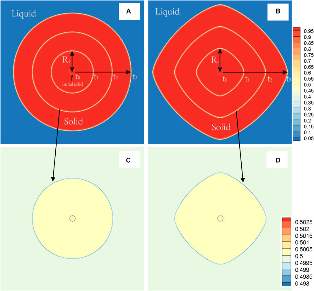
FIGURE 5. (color online) During the solidification process at 1800 K (TDB1), the solid phase morphology superimposed images at different times (t₀ = 0, t₁ = 300, t₂ = 600, t₃= 900) (A)δ = 0.0 (B)δ = 0.06, and representative image of the concentration field at the time of t₃, (C)δ = 0.0, (D)δ = 0.06. R₁ displays the definition of main radius at the time of t₁.

FIGURE 6

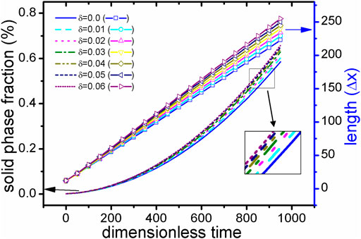
FIGURE 6. (color online) During the solidification process of TDB1 at 1800 K, the solid fraction (represented by different line types) and the main radius (represented by different lines + scattered points) under different anisotropic strengths δ over time. Particularly, a subset of solid phase fraction curves are enlarged in the picture.

Here, the velocity of R_main are further calculated for both cases of TDB1 and TDB2 to quantitatively characterize the effect of δ, as plotted in Figure 7. The absolute velocities corresponding to the two TDB files are obviously different, but in a similar linear relationship with the change of δ. The linear fitting slopes (in dimensionless unit), k^TDB1_v/δ∼ 0.572 and k^TDB2_v/δ∼ 0.338 show that the case of TDB1 is much more sensitive to anisotropy than that of TBD2, the difference of which is greater than 69%. The main reason for the significant difference between the two results is that the undercooling for TDB1 is much higher than that for TDB1 at the same 1800 K. Specifically, according to the original phase diagram corresponding to the two TDB files, it can be roughly estimated that the solidus and liquidus temperatures for TDB1 are 1867–1893 K, while those for TDB2 are 1821–1833 K with a given concentration 0.5. Therefore, the current interface-controlled transition can be attributed to relatively higher undercooling degree, especially for TDB1. If one intends to simulate dendrite growth by KKS model, the temperature should be chosen in the range of solid-liquid coexist region. The larger difference ΔT_SL between the solidus and liquidus temperature, the easier dendrites are produced, such as in the Al-Cu system (Choudhury et al., 2012). However, ΔT_SL for Fe-Cr is very small, particularly for TDB2, i.e., only about 15 K, resulting in difficulties in simulating the Fe-Cr dendrites. At this moment, it has to simulate crystal growth at different temperatures for TDB1 and TDB2, e.g., 1880 and 1827 K, respectively. δ is chosen to be 0.06, while keeping all the other kinetic parameters unchanged. Figure 8 exhibits the phase and concentration fields when their phase fraction is almost 30%. Surprisingly, the concentrations are clearly different whereas the two phase morphologies show much similarity with each other. Different from the previous one at 1800 K, this morphology shows a certain dendrite tip, which can be regarded as underdeveloped primary dendrite arm due to the limitation of simulation box and the small ΔT_SL (Qin and Bhadeshia, 2009). Moreover, the solute redistribution is more developed in TDB1 than that in TDB2, which is also consistent with their phase diagrams. Finally, the solid phase fraction and main radius changing with time are drawn in Figure 9. Unlike the counterpart at 1800 K, qualitatively, the phase fractions change almost linearly with time, and the main radii ∼t^1/2, one of typical characteristics for diffusion-controlled phase transition (Christian, 2002). Therefore, our program can accurately describe the differences in the microstructure caused by the small differences in the free energy via the KKS model (Li et al., 2007), capable of describing both of the interface- and diffusion- controlled phase transitions under the influence of interfacial anisotropy. In other words, the currently developed program can reasonably incorporate the thermodynamic data into the KKS model.

FIGURE 7

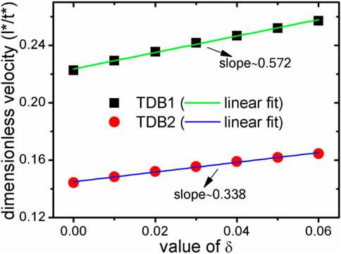
FIGURE 7. During the solidification process at 1800 K, the relationship between the main radius velocity of the solid phase and the anisotropic strength δ. The black square represents for TDB1, and the red circle for TDB2. The straight lines are their linear fitting lines. l* and t* denote the dimensionless length and time, respectively.

FIGURE 8

FIGURE 8. (color online) Snapshots of the microstructure displayed by phase field (A) TDB1 (B) TDB2 and concentration field (C) TDB1 (D) TDB2 at the same solid fraction as 30%.

FIGURE 9

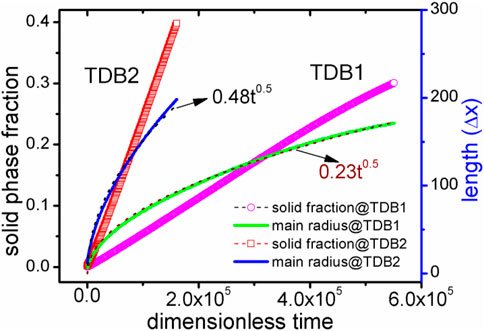
FIGURE 9. (color online) Solid phase fraction and main radius curves with time for the two TDBs. The dotted lines represent the results of nonlinear fitting using the formula R_main = kt^0.5.

Outlook

Quantitative phase field simulation of microstructure evolution has increasingly become a key factor limiting the implementation of the nuclear materials MGI. Some work is underway but more challenges need to be solved (Andreoni and Yip, 2020). By directly importing and analyzing TDB files, our new software tool eases the difficulty in automatically coupling thermodynamic data in PFMs, contributing to making the phase field models have system-specific predictive capabilities. It is expected to help activate the developers of phase field models in different communities to participate in the microstructural evolution simulation of nuclear materials. Furthermore, the software is highly expandable and can be further enriched for ternary systems and more physical mechanisms, such as diffusion kinetics, elasto-plasticity and the most important radiation effects. At present, there is no one exclusive phase field model that can consider so many factors at the same time. The feasible method consists of modifying phase field models to couple with many other methods on diverse length and time scales, which is likely to be realized with the help of MGI software platform. For example, a new multi-scale coupling platform that uses the phase field method as a meso-scale bridge to connect micro-simulation (i.e., DFT, MD) and macro-simulation (FEM) is being established by the authors, aiming at microstructural simulation and thermal-mechanical properties prediction of nuclear fuel cladding materials, including Fe-Cr-Al alloy (Liu et al., 2017). The establishment of the MGI software platform for nuclear materials requires many more methods, such as rate theory, cluster dynamics, crystal plasticity and so forth, which demands more work on the coupling of phase-field models with them in the future.

Conclusion

We have developed a new software tool PHAFIS for incorporating thermodynamic data into phase field modeling based on the CALPHAD method. The tool can automatically read and parse the standard TDB files, and accurately calculate the free energy and diffusion potential. Two versions of thermodynamic data of Fe-Cr alloys are employed to simulate spinodal decomposition and liquid-solid transition through the WBM and KKS phase field models, respectively. Our results show that even small deviation in the free energy may cause significant difference in the microstructure. Particularly, the program can accurately describe the interface- and diffusion-controlled phase transitions mechanisms under the influence of interfacial anisotropy via KKS model, consistent with relevant theories. PHAFIS makes it easy to achieve phase-field simulation coupled with thermodynamic data in an efficient way. The integrity of our phase field program paves the way for coupling more factors in microstructural evolution, and promotes the establishment of MGI software platform for alloys in nuclear reactors.

Data Availability Statement

The original contributions presented in the study are included in the article/Supplementary Material, further inquiries can be directed to the corresponding author.

Author Contributions

YG wrote the program and the draft of manuscript. YL parsed the format of TDB file and gave the ideas of program. ZL analyzed the research data and revised the paper. DS installed the OpenCalphad program and tested its feasibility. BZ deduced the solving method of phase field model and wrote the paper. JS organized and visualized part of the data of phase field simulation. MB analyzed the simulation data. SD supervised and provided the equipment, fundings and research ideas for this work and revised the manuscript.

Conflict of Interest

The authors declare that the research was conducted in the absence of any commercial or financial relationships that could be construed as a potential conflict of interest.

Acknowledgments

The authors acknowledge the financial support of the National Key Research and Development Program of China (No. 2016YFB0700100, 2019YFB1901001), the Zhejiang Province Key Research and Development Program (No. 2019C01060), National Natural Science Foundation of China (Grants No. 21875271, 21707147, 11604346, 21671195, 51872302), K.C.Wong Education Foundation (rczx0800), the Foundation of State Key Laboratory of Coal Conversion (Grant J18-19-301) the project of the key technology for virtue reactors from NPIC, and the defense industrial technology development program JCKY 2017201C016. We also acknowledge One Thousand Youth Talents Program of China, Hundred-Talent Program of Chinese Academy of Sciences.

References

Ahmed, K., Pakarinen, J., Allen, T., and El-Azab, A. (2014). Phase field simulation of grain growth in porous uranium dioxide. J. Nucl. Mater. 446, 90–99. doi:10.1016/j.jnucmat.2013.11.036

CrossRef Full Text | Google Scholar

Andersson, J.-O., Helander, T., Höglund, L., Shi, P., and Sundman, B. (2002). Thermo-Calc & DICTRA, computational tools for materials science. Calphad 26, 273–312. doi:10.1016/s0364-5916(02)00037-8

CrossRef Full Text | Google Scholar

Andreoni, W., and Yip, S. (2020). Handbook of materials modeling: Applications: Current and emerging materials. New York, United States: Springer.

Google Scholar

Braun, R., and Feller-Kniepmeier, M. (1985). Diffusion of chromium in α-iron. phys. stat. sol. (a) 90, 553–561. doi:10.1002/pssa.2210900219

CrossRef Full Text | Google Scholar

Byeong-Joo, L. (1993). Revision of thermodynamic descriptions of the Fe-Cr & Fe-Ni liquid phases. Calphad 17, 251–268. doi:10.1016/0364-5916(93)90004-u

CrossRef Full Text | Google Scholar

Cahn, J. W., and Hilliard, J. E. (1958). Free energy of a nonuniform system i interfacial free energy. J. Chem. Phys. 28, 258. doi:10.1063/1.1744102

CrossRef Full Text | Google Scholar

Chen, L.-Q. (2002). Phase-field models for microstructure evolution. Annu. Rev. Mater. Res. 32, 113–140. doi:10.1146/annurev.matsci.32.112001.132041

CrossRef Full Text | Google Scholar

Cheniour, A., Tonks, M. R., Gong, B., Yao, T., He, L., Harp, J. M., et al. (2020). Development of a grain growth model for u3si2 using experimental data, phase field simulation and molecular dynamics. J. Nucl. Mater. 532, 152069. doi:10.1016/j.jnucmat.2020.152069

CrossRef Full Text | Google Scholar

Choudhury, A., Reuther, K., Wesner, E., August, A., Nestler, B., and Rettenmayr, M. (2012). Comparison of phase-field and cellular automaton models for dendritic solidification in Al-Cu alloy. Comput. Mater. Sci. 55, 263–268. doi:10.1016/j.commatsci.2011.12.019

CrossRef Full Text | Google Scholar

Christian, J. W. (2002). The theory of transformations in metals and alloys. London, UK: Newnes.

Denton, A. R., and Ashcroft, N. W. (1991). Vegard's law. Phys. Rev. A 43, 3161–3164. doi:10.1103/physreva.43.3161

PubMed Abstract | CrossRef Full Text | Google Scholar

Dinsdale, A. T. (1991). Sgte data for pure elements. Calphad 15, 317–425. doi:10.1016/0364-5916(91)90030-n

CrossRef Full Text | Google Scholar

Eiken, J, Böttger, B, and Steinbach, I (2006). Multiphase-field approach for multicomponent alloys with extrapolation scheme for numerical application. Phys. Rev. E 73, 066122. doi:10.1103/physreve.73.066122

CrossRef Full Text | Google Scholar

Emmerich, H. (2008). Advances of and by phase-field modelling in condensed-matter physics. Adv. Phys. 57, 1–87. doi:10.1080/00018730701822522

CrossRef Full Text | Google Scholar

Ferreira, A. F., Silva, A. J. d., and Castro, J. A. d. (2006). Simulation of the solidification of pure nickel via the phase-field method. Mat. Res. 9, 349–356. doi:10.1590/s1516-14392006000400002

CrossRef Full Text | Google Scholar

Gale, WF, and Totemeier, TC (2004). Smithells metals reference book. Amsterdam, Netherlands: Elsevier.

Guo, Y., Liu, Z., Huang, Q., Lin, C.-T., and Du, S. (2018). Abnormal grain growth of uo2 with pores in the final stage of sintering: A phase field study. Comput. Mater. Sci. 145, 24–34. doi:10.1016/j.commatsci.2017.12.057

CrossRef Full Text | Google Scholar

Guthrie, R. I, and Iida, T. (1987). The physical properties of liquid metals. Oxford, United Kingdom: Clarendon press.

Hillert, M., and Jarl, M. (1978). A model for alloying in ferromagnetic metals. Calphad 2, 227–238. doi:10.1016/0364-5916(78)90011-1

CrossRef Full Text | Google Scholar

Hillert, M. (2001). The compound energy formalism. J. Alloys Compounds 320, 161–176. doi:10.1016/s0925-8388(00)01481-x

CrossRef Full Text | Google Scholar

Ingo, S (2009). Phase-field models in materials science. Modell. Simul. Mater. Sci. Eng. 17, 73031. doi:10.1088/0965-0393/17/7/073001

CrossRef Full Text | Google Scholar

Jacob, A., Povoden-Karadeniz, E., and Kozeschnik, E. (2018). Revised thermodynamic description of the Fe-Cr system based on an improved sublattice model of the σ phase. Calphad 60, 16–28. doi:10.1016/j.calphad.2017.10.002

CrossRef Full Text | Google Scholar

Kattner, U. R. (2016). The calphad method and its role in material and process development. Tecnol. Metal. Mater. Min. 13, 3. doi:10.4322/2176-1523.1059

PubMed Abstract | CrossRef Full Text | Google Scholar

Kim, S. G., Kim, W. T., and Suzuki, T. (1999). Phase-field model for binary alloys. Phys. Rev. E 60, 7186–7197. doi:10.1103/physreve.60.7186

CrossRef Full Text | Google Scholar

Kitashima, T. (2008). Coupling of the phase-field and calphad methods for predicting multicomponent, solid-state phase transformations. Philosophical Mag. 88, 1615–1637. doi:10.1080/14786430802243857

CrossRef Full Text | Google Scholar

Konings, R, and Stoller, RE (2020). Comprehensive nuclear materials. Amsterdam, Netherlands: Elsevier.

Li, J. J., Wang, J. C., Xu, Q., and Yang, G. C. (2007). Comparison of Johnson-Mehl-Avrami-Kologoromov (JMAK) kinetics with a phase field simulation for polycrystalline solidification. Acta Mater. 55, 825–832. doi:10.1016/j.actamat.2006.07.044

CrossRef Full Text | Google Scholar

Li, Y.-S., Li, S.-X., and Zhang, T.-Y. (2009). Effect of dislocations on spinodal decomposition in Fe-Cr alloys.J. Nucl. Mater. 395, 120–130. doi:10.1016/j.jnucmat.2009.10.042

CrossRef Full Text | Google Scholar

Li, Y, Hu, S, Sun, X, and Stan, M (2017). A review: Applications of the phase field method in predicting microstructure and property evolution of irradiated nuclear materials.Npj Comput. Mater. 3, 16. doi:10.1038/s41524-017-0018-y

CrossRef Full Text | Google Scholar

Liang, L., Kim, Y. S., Mei, Z.-G., Aagesen, L. K., and Yacout, A. M. (2018). Fission gas bubbles and recrystallization-induced degradation of the effective thermal conductivity in u-7mo fuels. J. Nucl. Mater. 511, 438–445. doi:10.1016/j.jnucmat.2018.09.054

CrossRef Full Text | Google Scholar

Liu, Z.-K., Chen, L.-Q., Raghavan, P., Du, Q., Sofo, J. O., Langer, S. A., et al. (2004). An integrated framework for multi-scale materials simulation and design. J. Computer-aided Mater. Des. 11, 183–199. doi:10.1007/s10820-005-3173-2

CrossRef Full Text | Google Scholar

Liu, Z., Li, Y., Shi, D., Guo, Y., Li, M., Zhou, X., et al. (2017). The development of cladding materials for the accident tolerant fuel system from the materials genome initiative. Scripta Mater. 141, 99–106. doi:10.1016/j.scriptamat.2017.07.030

CrossRef Full Text | Google Scholar

Liu, Z., Han, Q., Guo, Y., Lang, J., Shi, D., Zhang, Y., et al. (2019). Development of interatomic potentials for fe-cr-al alloy with the particle swarm optimization method. J. Alloys Compounds 780, 881–887. doi:10.1016/j.jallcom.2018.11.079

CrossRef Full Text | Google Scholar

Lübbehusen, M., and Mehrer, H. (1990). Self-diffusion in α-iron: The influence of dislocations and the effect of the magnetic phase transition. Acta Metallurgica et Materialia 38, 283–292. doi:10.1016/0956-7151(90)90058-o

CrossRef Full Text | Google Scholar

Lukas, H. L., Fries, S. G., and Sundman, B. (2007). Computational thermodynamics: The calphad method. Cambridge, UK: Cambridge University Press.

CrossRef Full Text

Mehrer, H. (2007). Diffusion in solids: Fundamentals, methods, materials, diffusion-controlled processes. Berlin, Germany: Springer Science & Business Media.

Mei, Z.-G., Liang, L., Kim, Y. S., Wiencek, T., O'Hare, E., Yacout, A. M., et al. (2016). Grain growth in U-7Mo alloy: A combined first-principles and phase field study. J. Nucl. Mater. 473, 300–308. doi:10.1016/j.jnucmat.2016.01.027

CrossRef Full Text | Google Scholar

Moelans, N., Blanpain, B., and Wollants, P. (2008). An introduction to phase-field modeling of microstructure evolution. Calphad 32, 268–294. doi:10.1016/j.calphad.2007.11.003

CrossRef Full Text | Google Scholar

Nestler, B., and Choudhury, A. (2011). Phase-field modeling of multi-component systems. Curr. Opin. Solid State. Mater. Sci. 15, 93–105. doi:10.1016/j.cossms.2011.01.003

CrossRef Full Text | Google Scholar

Neumann, G, and Tuijn, C (2011). Self-diffusion and impurity diffusion in pure metals: Handbook of experimental data. Amsterdam, Netherlands: Elsevier.

Peterson, N. L. S. F., Turnbull, D., and Ehrenreich, H. (1969). “Diffusion in metals,” in Phys. Solid state. (Cambridge, United States; Academic Press).

Google Scholar

Piochaud, J. B., Nastar, M., Soisson, F., Thuinet, L., and Legris, A. (2016). Atomic-based phase-field method for the modeling of radiation induced segregation in Fe-Cr. Comput. Mater. Sci. 122, 249–262. doi:10.1016/j.commatsci.2016.05.021

CrossRef Full Text | Google Scholar

Plapp, M (2011). Unified derivation of phase-field models for alloy solidification from a grand-potential functional. Phys. Rev. E 84, 31601. doi:10.1103/physreve.84.031601

CrossRef Full Text | Google Scholar

Qin, R. S., and Bhadeshia, H. K. D. H. (2009). Phase-field model study of the effect of interface anisotropy on the crystal morphological evolution of cubic metals. Acta Mater. 57, 2210–2216. doi:10.1016/j.actamat.2009.01.024

CrossRef Full Text | Google Scholar

Qin, R. S., and Bhadeshia, H. K. (2010). Phase field method. Acta Mater. 26, 803–811. doi:10.1179/174328409x453190

CrossRef Full Text | Google Scholar

Qin, R. S., and Wallach, E. R. (2003). A phase-field model coupled with a thermodynamic database. Acta Mater. 51, 6199–6210. doi:10.1016/s1359-6454(03)00443-9

CrossRef Full Text | Google Scholar

Redlich, O., and Kister, A. T. (1948). Algebraic representation of thermodynamic properties and the classification of solutions. Ind. Eng. Chem. 40, 345–348. doi:10.1021/ie50458a036

CrossRef Full Text | Google Scholar

Seeger, A. (1998). Lattice Vacancies in High-Purity α-Iron. Phys. Stat. Sol. (a) 167, 289–311. doi:10.1002/(sici)1521-396x(199806)167:2<289::aid-pssa289>3.0.co;2-v

CrossRef Full Text | Google Scholar

Shewmon, P (2016). Diffusion in solids. New York,United States: Springer International Publishers.

Steinbach, I., Böttger, B., Eiken, J., Warnken, N., and Fries, S. G. (2007). Calphad and phase-field modeling: A successful liaison. J Phs Eqil and Diff. 28, 101–106. doi:10.1007/s11669-006-9009-2

CrossRef Full Text | Google Scholar

Sundman, B., Jansson, B., and Andersson, J. -O. (1985). The thermo-calc databank system. Calphad 9, 153–190. doi:10.1016/0364-5916(85)90021-5

CrossRef Full Text | Google Scholar

Sundman, B., Kattner, U. R., Palumbo, M., and Fries, S. G. (2015). Opencalphad - a free thermodynamic software. Integrating Mater. 4, 1–15. doi:10.1186/s40192-014-0029-1

CrossRef Full Text | Google Scholar

Tonks, M. R., and Aagesen, L. K. (2019). The phase field method: Mesoscale simulation aiding material discovery. Annu. Rev. Mater. Res. 49, 79–102. doi:10.1146/annurev-matsci-070218-010151

CrossRef Full Text | Google Scholar

Tonks, M. R., Cheniour, A., and Aagesen, L. (2018). How to apply the phase field method to model radiation damage. Comput. Mater. Sci. 147, 353–362. doi:10.1016/j.commatsci.2018.02.007

CrossRef Full Text | Google Scholar

Turnbull, D. (1950). Formation of crystal nuclei in liquid metals. J. Appl. Phys. 21, 1022–1028. doi:10.1063/1.1699435

CrossRef Full Text | Google Scholar

van de Walle, A., Nataraj, C., and Liu, Z.-K. (2018). The thermodynamic database database. Calphad 61, 173–178. doi:10.1016/j.calphad.2018.04.003

CrossRef Full Text | Google Scholar

Wheeler, A. A., Boettinger, W. J., and McFadden, G. B. (1992). Phase-field model for isothermal phase transitions in binary alloys. Phys. Rev. A 45, 7424. doi:10.1103/physreva.45.7424

PubMed Abstract | CrossRef Full Text | Google Scholar

Wheeler, A. A., Boettinger, W. J., and McFadden, G. B. (1993). Phase-field model of solute trapping during solidification. Phys. Rev. E 47, 1893. doi:10.1103/physreve.47.1893

CrossRef Full Text | Google Scholar

Zhang, Y., Zuo, T. T., Tang, Z., Gao, M. C., Dahmen, K. A., Liaw, P. K., and Lu, Z. P. (2014). Microstructures and properties of high-entropy alloys. Prog. Mater. Sci. 61, 1–93. doi:10.1016/j.pmatsci.2013.10.001

CrossRef Full Text | Google Scholar

Zhang, L., Stratmann, M., Du, Y., Sundman, B., and Steinbach, I. (2015). Incorporating the calphad sublattice approach of ordering into the phase-field model with finite interface dissipation. Acta Mater. 88, 156–169. doi:10.1016/j.actamat.2014.11.037

CrossRef Full Text | Google Scholar

Zhu, J. Z., Liu, Z. K., Vaithyanathan, V., and Chen, L. Q. (2002). Linking phase-field model to calphad: Application to precipitate shape evolution in ni-base alloys. Scripta Mater. 46, 401–406. doi:10.1016/s1359-6462(02)00013-1

CrossRef Full Text | Google Scholar

Zinkle, S. J., and Was, G. S. (2013). Materials challenges in nuclear energy. Acta Mater. 61, 735–758. doi:10.1016/j.actamat.2012.11.004

CrossRef Full Text | Google Scholar