Machine Learning Techniques for the Segmentation of Tomographic Image Data of Functional Materials

In this paper, various kinds of applications are presented, in which tomographic image data depicting microstructures of materials are semantically segmented by combining machine learning methods and conventional image processing steps. The main focus of this paper is the grain-wise segmentation of time-resolved CT data of an AlCu specimen which was obtained in between several Ostwald ripening steps. The poorly visible grain boundaries in 3D CT data were enhanced using convolutional neural networks (CNNs). The CNN architectures considered in this paper are a 2D U-Net, a multichannel 2D U-Net and a 3D U-Net where the latter was trained at a lower resolution due to memory limitations. For training the CNNs, ground truth information was derived from 3D X-ray diffraction (3DXRD) measurements. The grain boundary images enhanced by the CNNs were then segmented using a marker-based watershed algorithm with an additional postprocessing step for reducing oversegmentation. The segmentation results obtained by this procedure were quantitatively compared to ground truth information derived by the 3DXRD measurements. A quantitative comparison between segmentation results indicates that the 3D U-Net performs best among the considered U-Net architectures. Additionally, a scenario, in which “ground truth” data is only available in one time step, is considered. Therefore, a CNN was trained only with CT and 3DXRD data from the last measured time step. The trained network and the image processing steps were then applied to the entire series of CT scans. The resulting segmentations exhibited a similar quality compared to those obtained by the network which was trained with the entire series of CT scans.

1. Introduction

In materials science, supervised machine learning techniques are used to describe relationships between the microstructure of materials and their physical properties (Stenzel et al., 2017; Xue et al., 2017). Roughly speaking, these techniques provide high-parametric regression or classification models. However, to analyze the microstructure and to determine quantitative descriptors for its morphology or texture, one often requires image acquisition techniques like X-ray microtomography or electron backscatter diffraction (EBSD). Therefore, image processing is necessary for analysis, which generally entails some sort of semantic segmentation of image data. The non-trivial task of segmentation can range from determining the material phases that are present in image data to the detection and extraction of single particles, grains or fibers. The quality of the segmentation has a significant influence on the subsequent analysis of the material's microstructure and macroscopic physical properties.

Thus, in the present paper, we focus on machine learning techniques that provide assistance in the segmentation of image data. In recent years, numerous approaches for various fields have been considered that deal with this issue, where specifically convolutional neural networks (CNNs, Goodfellow et al., 2016) enjoy an increased popularity. In the field of object detection in 2D images the Region-CNN (R-CNN, Girshick et al., 2014) was successfully used for determining bounding boxes around objects of interest. In recent years this architecture was enhanced, resulting in the Fast R-CNN (Girshick, 2015) and Faster R-CNN (Ren et al., 2017). However, in many applications it does not suffice to obtain a bounding box around objects of interest—a much finer segmentation was achieved by He et al. (2017) who extended the Faster R-CNN architecture to assign image pixels to object instances detected in 2D image data. Recently, another CNN architecture, namely the U-Net (Ronneberger et al., 2015) was used for the segmentation of biomedical 2D image data. In later works, variations of the U-Net were introduced which are able to process and segment volumetric image data, see Çiçek et al. (2016) and Falk et al. (2019). Furthermore, conventional segmentation techniques, like the watershed transform (Beucher and Lantuéjoul, 1979), have been utilized in combination with methods from machine learning in segmentation tasks, see Naylor et al. (2017) and Nunez-Iglesias et al. (2013).

In the present paper, we give a short overview of several applications in the field of materials science in which we successfully combined methods of statistical learning—including random forests, feedforward and convolutional neural networks—with conventional image processing techniques for segmentation, classification and object detection tasks, see e.g., Furat et al. (2018), Neumann et al. (2019), and Petrich et al. (2017). This shows the flexibility of the approach of combining conventional image processing with machine learning techniques, where the latter can be used either for preprocessing image data to increase the performance of conventional image processing algorithms or for postprocessing segmentations obtained by conventional means in order to improve segmentation qualities.

Based on our experience from previous studies, we apply similar techniques to the segmentation of time-resolved tomographic image data of polycrystalline materials. More precisely, the focus of the present paper is on data of an AlCu alloy that was repeatedly imaged by X-ray computed tomography (CT) following periods of Ostwald ripening. In order to investigate the relationship between grain geometry and functional properties, the study of grain boundary movement—caused by the growth of grains during the ripening process—is of particular interest (Werz et al., 2014). Therefore, it is necessary to segment the CT image data into single grains. Due to the poor visibility of grain boundaries at high volume fractions in CT data (Werz et al., 2014), this task is demanding, especially when targeted using conventional image processing approaches.

Consequently, we will utilize convolutional neural networks, in particular architectures based on the U-Net (Ronneberger et al., 2015), for enhancing and predicting grain boundaries from CT data obtained after several ripening steps. More precisely, we use single- and multichannel U-Nets which receive 2D input and can be applied slice-by-slice to image stacks. Additionally, we trained a 3D U-Net which can evaluate volumetric data at a lower resolution, due to higher memory consumption. For training the neural networks we use “ground truth” information derived from 3D X-ray diffraction (3DXRD) microscopy, which allows grains and their boundaries to be extracted from the technique's measurement of local crystallographic orientation. The trained networks can then recover grain boundaries of poor visibility in CT data reasonably well, without drawing on additional 3DXRD information.

The rest of this paper is organized as follows. In section 2, we give a short overview of some applications that combine machine learning methods with conventional techniques of image processing for the semantic segmentation and classification of image data. Section 2.1 deals with the trinarization of the microstructure of Ibuprofen tablets using random forests and the watershed algorithm (Neumann et al., 2019). Then, in section 2.2, particulate systems of minerals are considered that are of interest in the mining industry. Here, a feedforward neural network is used to refine particle-wise segmentations obtained from the watershed algorithm (Furat et al., 2018). The watershed algorithm and feedforward neural networks are also combined in section 2.3. However, in the latter case, the focus lies on the detection of particle cracks in the 3D microstructure of lithium-ion batteries (Petrich et al., 2017).

The main results of the present paper are given in section 3. To begin with, in section 3.1, we describe the problem at hand when considering CT image data of AlCu alloys. In section 3.2, we utilize 3DXRD microscopy data to train three neural networks to extract grain boundaries from CT image data: a 2D U-Net for slice-by-slice evaluation, a multichannel 2D U-Net which can process consecutive slices and a 3D U-Net which uses full 3D information at a lower resolution. The grain boundary predictions of these networks are then segmented into single grains with conventional image processing tools (Spettl et al., 2015). In section 3.3, we quantitatively compare the presented methods by matching segmented grains to the “ground truth” obtained by 3DXRD measurement. Then, in section 3.4 we discuss how similar approaches can be utilized in other fields in which “ground truth” measurements are not easily feasible. Finally, section 4 concludes.

2. Overview of Previous Results

In this section, we give a short overview of different applications in the field of materials science in which we successfully combined methods of statistical learning, including random forests, feedforward and convolutional neural networks with conventional image processing techniques for segmentation, classification and object detection tasks.

2.1. Segmentation of Ibuprofen Tablets

In Neumann et al. (2019), a hybrid algorithm combining machine learning techniques with conventional tools of image analysis has been used to trinarize tomographic image data representing the microstructure of Ibuprofen tablets, i.e., to classify each voxel of the grayscale image as one of the three phases the tablet consists of. These phases are microcrystalline cellulose (MCC), Ibuprofen (API) and pores. In the following, we describe the challenges of this particular trinarization problem and briefly summarize the developed hybrid trinarization algorithm. Moreover, we discuss to which extent it improves the algorithms which are based either on machine learning techniques or on conventional image analysis. For details, we refer to Neumann et al. (2019).

A 2D slice of the 3D image data, which is obtained by synchrotron tomography and represents the microstructure of Ibuprofen tablets, is visualized in Figure 1. The image data consists of cubic voxels with a side length of 0.438 μm, while the resolution limit is at about 2 μm. Although there is a good contrast between the three constituents of the tablets, it is challenging to perform an algorithmic tinarization, mainly due to the following two aspects. First, the grayscale values of some voxels within MCC are in the same range as the grayscale values of those voxels which belong clearly to API. Second, long thin pores occur at the boundary of MCC particles, the corresponding grayscale values of which are similar to the ones of API. These two aspects suggest that in this application it is not reasonable to rely only on thresholding of grayscale values in order to obtain a physically coherent trinarization.

FIGURE 1

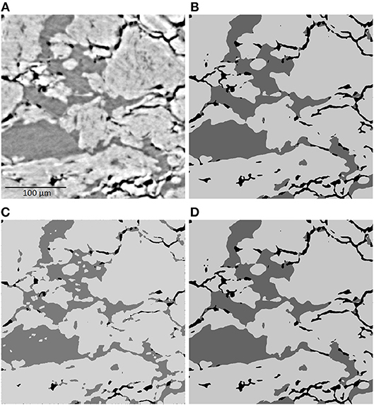
Figure 1. 2D slice of a cutout of the grayscale image (A) and the corresponding results of the three different trinarization algorithms, namely the trinarization by statistical learning (B), by the aid of a watershed algorithm (C), and by a hybrid approach (D). In the trinarized images (B–D), black, dark gray and bright gray indicate the pore space, API and MCC, respectively.

To deal with these challenges by means of machine learning, a random forest algorithm is used, i.e., a classification algorithm is considered which is based on a large number of randomized decision trees (James et al., 2013). To train the random forest algorithm, N voxels of a 2D slice of the image are manually classified by visual inspection. On the same 2D slice, M different filters are applied. Doing so, we obtain for each of the N manually classified voxels, an (M + 1)-dimensional feature vector. It contains the original grayscale value of the voxel as well as the M grayscale values after application of the M filters. The random forest is trained to classify the voxels, i.e., to trinarize the image, by means of these feature vectors. For this purpose, Ilastik (Sommer et al., 2011) is used in combination with the parallelized random forest implemented in the computer vision library VIGRA. The results of the random forest algorithm are visualized in Figure 1B. One can observe that it leads to a satisfactorily well trinarization. Regarding the challenges mentioned above, the random forest algorithm leads to a good classification of MCC particles, even if an occurrence of API inside them is suggested by small grayscale values. Moreover, the long and thin pores at the boundary of MCC particles are reflected well in the trinarized image, since the algorithm is trained to detect such thin pores. However, this leads to wrongly detected pore voxels at the boundary between MCC and API when there is no indication for pores, neither by grayscale values nor by physical reasons. This effect can be removed by combining the random forest algorithm with a trinarization which is based on conventional image analysis and using the watershed algorithm.

The main idea of the watershed-based trinarization is as follows. At first, the pore space is determined via global thresholding. Here the threshold value is manually chosen by visual inspection. In the second step, regions, in which the deviation of grayscale values is relatively small, are determined by the watershed algorithm (Beucher and Lantuéjoul, 1979; Meyer, 1994; Beare and Lehmann, 2006). Then, each of these regions is either classified as API or MCC according to their average grayscale values. The results of the watershed-based trinarization, visualized in Figure 1, shows that this approach leads to an appropriate trinarization, when only the grayscale values are considered without any additional physical information about the material. But, the random forest trinarization is significantly better with respect to the detection of MCC particles and long, thin pores. Nevertheless, the watershed-based trinarization does not detect unrealistic pores at the boundary between API and MCC. Thus, the information obtained by the watershed-based trinarization can be used to further improve the random forest trinarization.

In particular, each pore voxel v of the random forest trinarization is relabeled as API voxel if the closest pore voxel in the watershed-based trinarization has a distance of more than 8.76 μm and the closest voxel classified as API in the random forest trinarization has a distance of at most 8.76 μm. The latter condition is necessary since pores within MCC, which are not detected by the watershed-based trinarization should not be removed. The value of 8.76 μm is manually chosen and is justified by visual inspection of the obtained result. A 2D slice of the final trinarization is shown in Figure 1D. The combination of the random forest trinarization with the watershed-based trinarization meets the required challenges of classifying the three constituents of Ibuprofen tablets. Based on the trinarized image, a characterization of the 3D microstructure of Ibuprofen tablets is performed by means of spatial statistics in Neumann et al. (2019).

2.2. Segmentation of Mineral Particle Systems

In the previous section, we discussed how to combine tools of conventional image processing with machine learning techniques to determine the material's phases in tomographic image data. However, in many applications a much finer segmentation is required, e.g., for tomographic images of particle or grain systems the segmentation has to correctly separate these objects from the background and from each other. For such segmentation problems, modified versions of the watershed algorithm, which entail some sort of pre- or postprocessing of image data, often yield good results (Roerdink and Meijster, 2000; Rowenhorst et al., 2006b; Spettl et al., 2015; Kuchler et al., 2018). The preprocessing steps are necessary to determine unique markers for each particle or grain, from which the watershed algorithm grows regions which lead to a segmentation of the image. A carefully adjusted marker detection is required: If multiple markers are determined in a single particle, the watershed splits the particle into multiple fragments, see Figure 2B. This issue is referred to as oversegmentation. On the other hand, too few markers lead to a segmentation, in which multiple particles are assigned to a single region. The marker detection is especially difficult if the particles depicted in the image data have irregular, for example elongated or plate-like, shapes. Therefore, a postprocessing step is required to correct the mentioned issues, e.g., by merging regions to overcome oversegmentation.

FIGURE 2

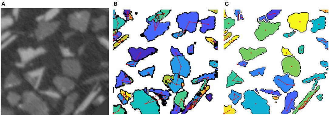
Figure 2. (A) 2D cut-out of tomographic image data of ore particles. (B) Oversegmented image obtained by the watershed transformation. Red lines are set between adjacent regions. Note that some regions are adjacent in 3D but not in the visualized planar section. (C) Segmentation after a postprocessing step using a neural network.

In Furat et al. (2018) X-ray microtomography (XMT) image data of a mixture of particles was considered. These particles comprise of ores and other minerals and have a size of about 100 μm, see Figure 2A. In order to analyze particle properties from such image data, for example, the distributions of volume or some shape characteristics, one needs to extract single particles from image data via segmentation. However, the watershed algorithm often fails for the considered data, since, for example, elongated particles are segmented into multiple fragments. In Furat et al. (2018) a postprocessing step was described which utilizes machine learning techniques, more precisely a feedforward neural network, to eliminate oversegmentation.

Therefore, an oversegmented image I_over of a tomographic grayscale image I of the sample under consideration, was represented by an undirected graph G = (V, E), where each vertex v ∈ V represents a region of the oversegmented image I_over. Furthermore, the set E contains an edge e = (v₁, v₂) between two vertices v₁, v₂ ∈ V if the corresponding regions are adjacent in the oversegmented image I_over. The goal of the neural network was the elimination of edges between adjacent regions which belong to different particles, while preserving those which lie in the same one. This lead to a reduced set of edges Ẽ⊂E. A remaining edge (v₁, v₂) ∈ Ẽ indicated that the corresponding adjacent regions should be merged in the oversegmented image. For the neural network to decide whether to remove an edge e ∈ E, it required input, in form of feature vectors $x_e\in {ℝ}^p$, obtained from the original grayscale image I.

Among the components of the input vectors x_e, local contrast information was stored. More precisely, the absolute gradient image of I was computed using Sobel operators, see Soille (2013). For an edge e = (v₁, v₂) the voxels in the vicinity of the interface between the two regions surrounding the vertices v₁ and v₂ were considered for the computation of the first four moments of the absolute gradient values in this local neighborhood. These values were stored in the feature vector x_e. Furthermore, x_e was appended with the relative frequencies of the histogram of the local absolute gradient values. Analogously, local information of the first four moments and relative frequencies of the histogram of local grayscale values of the original image I were stored in x_e. Note that the previously described features of the vector x_e contain only local contrast information. Therefore, some local geometry features were included in a similar manner. By computing local curvatures, the first four moments and histogram frequencies of curvatures were obtained in the vicinity of the interface between v₁ and v₂. Another geometrical feature which was considered, characterizes the shape of the interface itself. More precisely, a principle component analysis (PCA) of the voxels (Hastie et al., 2009), which form the interface between the adjacent regions, was performed. The eigenvalues obtained by the PCA were stored in the feature vector x_e.

Then the classification problem was formulated as

$\begin{array}{ll}f(x_e)=\{\begin{array}{ll}1,\hfill & \text{ if }{v}_1,v_2\text{ belong to the same particle,}\hfill \\ 0,\hfill & \text{ else, }\hfill \end{array}& (1)\end{array}$

for each edge e = (v₁, v₂) ∈ E. As a model for the classifier f a feedforward network was chosen and the target values for feature vectors x_e were determined by manually segmenting a small cut-out of the image data. The trained network f was then used to classify which edges e should be removed, i.e., edges with f(x_e) = 0. Figure 2B depicts the initial graph, in which edges are set between adjacent regions. After the edge reduction with the neural network, regions connected by an edge e with f(x_e) = 1 get merged, thus leading to a less oversegmented system of particles, see Figure 2C.

2.3. Crack Detection in Lithium-Ion Cells

In sections 2.1 and 2.2, machine learning is applied to image segmentation problems. In this section we present an approach that goes one step further and employs similar techniques, but instead of identifying individual particles, the relationship between two particles is investigated, which allows to localize regions of interest in electrodes of lithium-ion batteries.

Lithium-ion batteries are among the most commonly used types of batteries since they combine several beneficial properties, such as high energy density and low self-discharge. However, one of their biggest disadvantages is their vulnerability to thermal runaway caused, e.g., by overheating or overcharging, which can lead to disastrous incidents like fires or even explosions. An active research field deals with the design of lithium-ion batteries with minimal risk of failure. It is known that during thermal runaway the particles in the electrode material break (Finegan et al., 2016), and the resulting increase in surface area intensifies the heat generation (Jiang and Dahn, 2004; Geder et al., 2014). However, many questions are still unanswered and an in-depth analysis on how the microstructure of the electrodes affects the safety of the battery requires information on the locations of the broken particles in post-mortem cells.

For this purpose, in Petrich et al. (2017) a method is presented that allows an automatic detection of particle cracks in tomographic image data of lithium-ion batteries and thus reduces the amount of manual labeling, which is tedious at best or outright infeasible for large datasets. More precisely, a commercial LiCoO₂ cell was overcharged, which led to a thermal runaway. The post-mortem sample was imaged in a lab-based X-ray nano-CT system and to prepare the data for further analysis it was denoised, binarized, and individual particles were segmented. In Petrich et al. (2017), pairs of adjacent particles are considered and categorized in one of the following classes.

• The particle pair belonged to the same particle in the real microstructure, but it broke apart during the thermal runaway. (BROKEN)

• The particle pair is actually a single particle in the tomographic image, but it was split during the image preprocessing. (PREPROCESSSEP)

• The particle pair consists of unrelated, separate particles, i.e., a pair which is neither BROKEN nor PREPROCESSSEP. (PARTICLESEP)

The goal is to automatically classify pairs of particles with methods from machine learning, which require hand-labeling only for a small subset of the data. In the presented case, an expert labeled 294 particle pairs. An important part of many machine learning applications is to translate the problem at hand to quantitative features. In order to facilitate this feature engineering step, synthetic data was used, for which it is possible to generate arbitrarily many particle pairs and their true class labels. This means that the quality of several features on a bigger artificial dataset (3693 instances) was investigated by training many different classification models and evaluating their performance. The best features were selected and a new model was trained and tested on the hand-labeled dataset, which was used for validation. An overview of the approach is visualized in Figure 3.

FIGURE 3

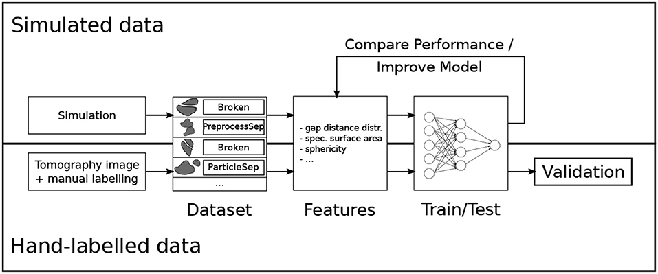
Figure 3. Overview of the model development for the crack detection in lithium-ion batteries. Reprinted from Petrich et al. (2017), Figure 1, with permission from Elsevier.

For the simulated dataset, first, a system of individual pristine particles was generated based on the stochastic microstructure model introduced in Feinauer et al. (2015a) and Feinauer et al. (2015b), then a certain percentage of particles were broken in two parts as described in Petrich et al. (2017). The individual particles were discretized in a single 3D image and the same image preprocessing was performed as on the tomographic image data. Because in each step—the particle creation, the breakage, and the image preprocessing—the relationships of the particles to their neighbors were tracked, it is possible to generate a list of particle pairs and their true class label. This list was subsampled such that there were the same number of instances for each class.

Based on this simulated dataset numerical features were designed. For these, not only the individual particles were considered, but also a combination of the two, which here means the morphological closing (Soille, 2013) of the two particles. Some features are straight forward, like the fraction of the volume of the smaller particle to the volume of the larger one or the volume of the combined particles divided by the sum of the individual volumes. The same ratios were calculated for the surface area. The next quantity is more complicated, but also showed more predictive power. Here, for each voxel on the boundary of the particles the distance to the other particle is computed and the histogram of these values forms another (multidimensional) feature.

As in section 2.2 for the classification a multilayer perceptron (MLP), i.e., a feed-forward neural network with one hidden layer, was chosen. For an introduction to MLPs and machine learning in general, see Bishop (2006) and Hastie et al. (2009). The input for the classifier was the standardization of the feature vector described above. The sigmoid function is used for the non-linear activation functions in the input and hidden layer, and the softmax function for the output layer. The network was trained with the quasi-Newton method L-BFGS (Nocedal and Wright, 2006), which minimizes the cross-entropy loss with L₂ regularization. The hyperparameters (i.e., number of hidden neurons and weight of the L₂ regularization term) were tuned with a 5-fold stratified cross-validation maximizing the accuracy.

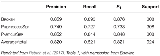
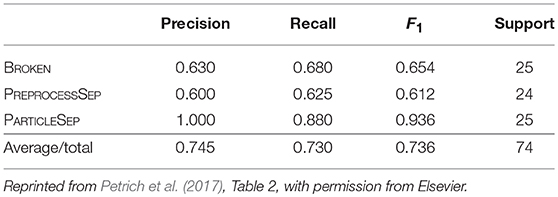
With this setup two classifiers were built, one for the simulated and one for the hand-labeled dataset. In each set 75% of the instances were used to train the classifier and the rest to evaluate its performance. The results for the simulated dataset (2769 samples for training, 924 for testing) are shown in Table 1. The overall accuracy is 82.1%. The evaluation results for the hand-labeled data (220 samples for training, 74 for testing) are presented in Table 2. Here, the classifier achieved an accuracy of 73.0%.

TABLE 1

Table 1. Performance metrics for the classifier based on the simulated test data.

TABLE 2

Table 2. Performance metrics for the classifier based on the hand-labeled test data.

All in all, a good prediction performance is observed. It is not surprising that the hand-labeled data is harder to classify than the simulated dataset since especially the breakage algorithm gives only an approximation to the real degraded microstructure of the electrode of a lithium-ion battery. However, the similarity of the results shows that it is a valid strategy to perform the feature engineering on the simulated dataset. As it can be seen in Table 2, the classifier mostly struggles with separating PREPROCESSSEP and BROKEN classes, but this is hard, even for humans, as can be seen in Figures 4B,C. Further examples of particle pairs with their true and predicted classes are depicted in Figure 4.

FIGURE 4

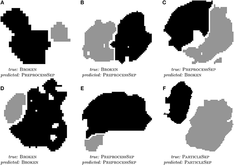
Figure 4. 2D slices of three misclassified (A–C) and three correctly classified (D–F) examples of particle pairs from the hand-labeled dataset with their true and predicted class label. Reprinted from Petrich et al. (2017), Figure 11, with permission from Elsevier.

3. Segmentation of Time-Resolved Tomographic Image Data

3.1. Description of the Problem

Tomographic image data of materials provides extensive information regarding microstructure, from which the latter's influence on a given sample's functional properties can be assessed. However, in most applications, this type of analysis becomes possible only after successful segmentation of the image data. Moreover, for some materials it can be difficult to obtain adequate CT data for analysis—for example, when the material is comprised of phases covering a broad spectrum of mass densities, which can lead to beam-hardening artifacts. Other issues can occur when a given specimen is homogeneous in density or X-ray attenuation, which causes low contrast in the resulting image data. The latter is a challenge in the case of polycrystalline materials, for which the grain microstructure manifests itself through heterogeneities in crystallographic orientation. The interfaces between neighboring grains, which are called grain boundaries, give rise to such small changes in X-ray attenuation that the boundaries are invisible to standard (i.e., absorption-contrast) CT measurements. Consequently, techniques that exploit other grain-to-grain contrast mechanisms—such as 3D electron backscatter diffraction (3DEBSD) or 3DXRD microscopy—must be utilized to image single-phase polycrystalline materials (Rowenhorst et al., 2006a; Bhandari et al., 2007; Schmidt et al., 2008; Poulsen, 2012).

Alternatively, if a particular material has a two-phase region in which one phase decorates the grain boundaries of the other phase, then it may be possible to map out the network of grain boundaries directly using only CT. For example, in Werz et al. (2014), tomographic measurements were performed on an Al-5 wt.% Cu alloy at various stages of Ostwald ripening, during which a liquid layer of a minority phase was present between the grains of the solid majority phase. X-ray absorption contrast arose from the higher concentration of Cu in the liquid than in the solid phase; this contrast was easily visible in CT reconstructions of the characterized volume, see Figure 5A. The subsequent image analysis is described in Spettl et al. (2015), in which modified conventional image processing techniques were employed to perform a grain-wise segmentation of the considered image data.

FIGURE 5

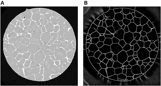
Figure 5. (A) Two-dimensional cross-section of a CT reconstruction of Al-5 wt.% Cu with 7% (by volume) of liquid phase; the lighter gray pixels correspond to liquid regions located mainly at the boundaries between solid grains (darker gray pixels). (B) The corresponding output of a U-Net which was trained with 2D cross sectional images.

Although the liquid phase is responsible for making the polycrystalline microstructure visible to X-ray tomography, the liquid itself can interact strongly with the network of grain boundaries, thereby exerting a non-negligible influence on the equilibrium shape of grains or on the migration kinetics of boundaries during Ostwald ripening. For this reason, we consider the analysis of CT image data for an Al-5 wt.% Cu alloy containing only 2% (by volume) of the liquid phase. This sample was imaged a total of seven times by CT; between each measurement the specimen experienced 10 min of Ostwald ripening.

From here on, we refer to the resulting 3D images as C₀, …, C₆, see Figure 8 (left column). Note that the grain boundaries become less distinct during the Ostwald ripening process, which exacerbates the difficulty of segmenting individual grains by standard image processing algorithms. Therefore, we turn our attention to machine learning techniques, namely convolutional neural networks (CNNs) (Goodfellow et al., 2016), to extract grain boundaries from the tomographic images C_t. In contrast to the method described in section 2.2, in which a neural network was used as a postprocessing step to refine a segmentation, CNNs are employed in the present section as a preprocessing step to enhance and predict grain boundaries. Another key difference between the methods described here and in sections 2.2 and 2.3 is that the present CNNs do not require user-defined image features for their decision making, but are able to determine their own features. More precisely, the trainable parameters of a CNN are discrete kernels that can detect (depending on the kernel size) local features via convolution with input images. The aggregation of such local features allows the detection of larger-scale features. Thus, CNNs are capable of learning and incorporating multi-scale features into their decision-making process.

3.2. Materials and Methods

Like every supervised machine learning technique, CNNs require training data in form of pairs of input and desired target images. In the context of the present paper, this means that for each 3D image obtained by CT we require a corresponding 3D image in which the grain boundaries have already been extracted. Such grain boundary images were obtained by an additional image acquisition technique: at each imaging step t = 0, …, 6, in addition to CT measurements (C_t) the same sample volume was characterized by 3DXRD microscopy. This paired information will be used to train CNNs such that they are able to predict grain boundaries from CT image data without additional 3DXRD imaging. Now, we provide additional details regarding the nature of the data, the chosen CNN architectures and the training procedure.

Both CT and 3DXRD measurements were carried out on Al-5 wt. % Cu at beamline BL20XU of the synchrotron radiation facility SPring-8. The sample had a cylindrical shape with a diameter of 1.4 mm. Mounted on a rotating stage, it was illuminated by a monochromatic X-ray beam with an energy of 32-keV. We recorded both far-field and near-field diffraction patterns on 2D detectors. Followed the reconstruction routine described in Schmidt et al. (2008) and Schmidt (2014), the grain morphology together with the crystallographic orientation of individual grains was mapped. Heat treatment of the sample took place at 575°C, at which temperature the microstructure consisted of a mixture of solid and liquid phases according to the Al-Cu phase diagram (Massalski, 1996). Under these conditions, the sample undergoes slow but steady Ostwald ripening. After an annealing time of 10 min, the sample was cooled to room temperature and characterized by both CT and 3DXRD microscopy. In total, the specimen was held for 60 min at 575°C and mapped seven times. Due to small misalignments that occurred each time the sample was removed from the X-ray beamline for annealing, it was necessary to register sequential CT and 3DXRD measurements according to the method described in Dake et al. (2016).

Reconstruction and processing of the 3DXRD data yielded the local crystallographic orientation, from which segmented 3D images of grains and thus grain boundary images L_t were obtained (Schmidt, 2014), see Figures 6B,C. Since the state of the specimen did not change between CT and 3DXRD measurements, the images L_t derived from the latter depict the true grain boundary systems of the corresponding reconstructed CT images C_t, for each t = 0, ⋯ , 6. The CT images C_t had a size of 960 × 960 × 1678 voxels, with cubic voxels of size 0.75μm.

FIGURE 6

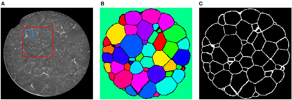
Figure 6. (A) Cross-section of C₂ depicting the sample after 20 min of Ostwald ripening. These images will be used as training input for the CNN. The blue square indicates the size of an 80 × 80 cutout with respect to the original resolution of the CT data. After downsampling the data to the resolution of 240 × 240 × 420 voxels an 80 × 80 cutout has the relative size indicated by the red square. (B) Segmentation of the corresponding section obtained via 3DXRD microscopy. (C) Cross-section of the extracted grain boundary image L₂ from the 3DXRD data. The grain boundary images L_t will be used as target images for the input images C_t during training of the CNN.

Due to the registration step of CT and 3DXRD measurements the grain boundaries visible in C_t are aligned with those of L_t for each t = 0, ⋯ , 6. A cross-section of such a matching pair is visualized in Figures 6A,C. As a consequence, we can formulate the issue of detecting grain boundaries from CT images as a regression problem. More precisely, we seek a function f with

$\begin{array}{ll}f(C_t)\approx L_t,& (2)\end{array}$

for each 3D CT image C_t with values in the interval [0, 1] and the corresponding binary grain boundary image L_t with values in {0, 1}, with 1 indicating grain boundaries and 0 grain interiors.

As regression models for the function f we use CNNs based on the U-Net architecture. In recent years, this architecture has been used successfully in several segmentation tasks, see Çiçek et al. (2016) and Ronneberger et al. (2015). The U-Net uses several max-pooling layers, which downsample the image data. Then, even small kernels applied to downsampled data can detect large-scale features—see Figure 7 for the architecture of the considered U-Net with volumetric input. In order to inspect the capabilities of the U-Net architecture, we used CT measurements of an Al-5 wt% Cu sample having a liquid content of 7% (thus grain boundaries with a good visibility) to train such a neural network to handle two-dimensional input images. Figure 5 indicates that this U-Net can predict the location of grain boundaries, even when they are not visible in CT data. This visual inspection of the results obtained for 2D input images motivates the use of a U-Net for three-dimensional CT images of such materials with the low liquid content of 2%, see Figure 8 (left column).

FIGURE 7

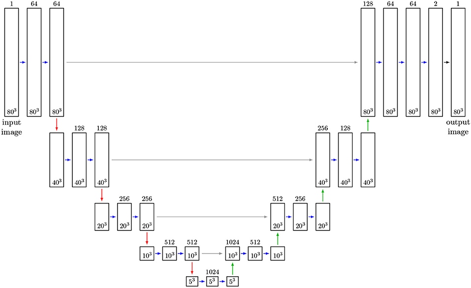
Figure 7. Adapted 3D U-Net architecture (Ronneberger et al., 2015): Feature maps are represented by boxes, where the number of channels is indicated by the number above the box. Blue arrows indicate convolutional layers with kernel size of 3 × 3 × 3 and ReLu activation functions. Red arrows describe max-pooling layers of size 2 × 2 × 2. Up-convolutional layers of size are 2 × 2 × 2 indicated by green arrows. Merge layers are visualized by gray arrows. The layer (black arrow) generating the output is a convolutional layer with kernel size 1 × 1 × 1 and a sigmoid activation function. The sizes of input, feature and output images during training is given in the boxes. After training the network can receive arbitrarily sized images as input, provided their size in each direction is a multiple of 2⁴ = 16.

FIGURE 8

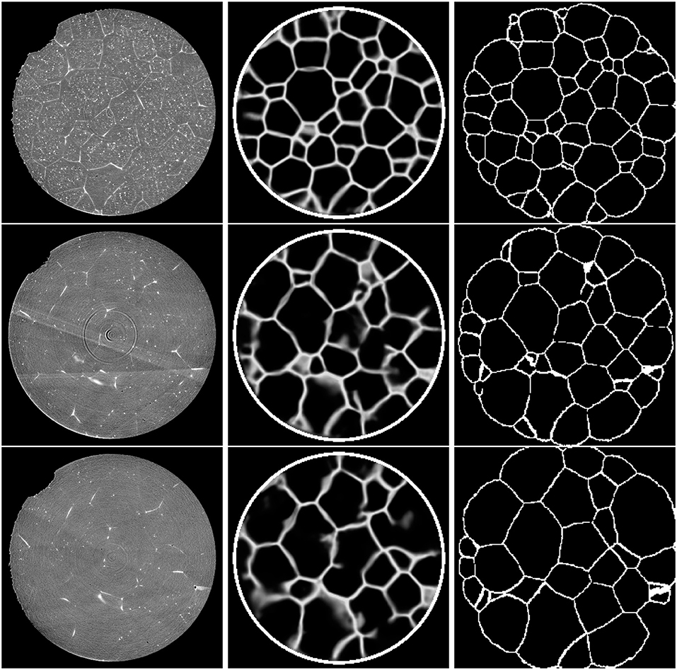
Figure 8. Cross-sections (slice 350) of the 3D CT input images (Left column). Corresponding sections of the output of the trained 3D U-Net (Middle column). Note that the white circle surrounding the specimen was added in a separate image-processing step. Ground truth obtained by 3DXRD microscopy (Right column). First row: Initial state of the sample (t = 0). Second row: Sample after three time steps. Third row: Sample after six time steps.

Now, we describe the architecture of the chosen 3D U-Net for detecting grain boundaries in 3D data. A size of 3 × 3 × 3 for the trainable kernels of the 3D U-Net depicted in Figure 7 was chosen. The activation functions of the 3D U-Net's hidden layers are rectified linear unit (ReLU) functions (Glorot et al., 2011), and for the output layer a sigmoid function was chosen, such that the voxel values of output images are normalized to values in the interval (0, 1). Due to memory limitations the training could only be performed on cutouts from the images C_t and L_t with a size of 80 × 80 × 80 voxels. Since these cutouts cover relatively small volumes, see Figure 6A, they do not provide the necessary size for learning large scale features with the 3D U-Net. In order to remedy this, the CT image data was downsampled from 960 × 960 × 1678 voxels to 240 × 240 × 420 voxels, with some manageable loss of information. Analogously, we upsampled the corresponding grain boundary images L_t, which initially had a voxel size of 5 μm, to obtain the same voxel and image size. For simplicity, we denote the resampled CT and grain boundary images by C_t and L_t, respectively. Then, training was performed on cutouts with 80 × 80 × 80 voxels, which can represent larger grain boundary structures at this scale after downsampling, see Figure 6A. The cutouts were taken randomly from the images C_t and the corresponding sections of the grain boundary images L_t. Note that, in contrast to the U-Net architecture proposed in Ronneberger et al. (2015), we padded the convoluted images of the CNN such that input and output images have the same size. Thus, the network's input is not restricted to images with a size of 80 × 80 × 80 voxels, i.e., it can be applied to the entire scaled CT image stack (240 × 240 × 420 voxels) after training. The only limitation is that the number of voxels in each direction of the input images must be a multiple of 2⁴ = 16, which can be achieved by padding the image stack. This constraint arises from the four 2 × 2 × 2 max-pooling layers—which downsample images—followed by the four up-convolutional layers, see Figure 7. The number of max-pooling layers, which we call the depth of the U-Net in the following, can be increased such that the network can learn features of a larger scale. Note that in this case, the numbers of convolutional, up-convolutional and merge layers are adjusted accordingly. Furthermore, we point out that the cutouts used for training were taken from image data among all seven time steps, but only from the first 200 slices of each image stack; thus, the remaining 220 slices could be used for validation and testing. In order to increase the efficiency of the available training data, we utilized data augmentation (Goodfellow et al., 2016)—i.e., during training, pairs of chosen input and corresponding target cutouts were transformed randomly, yet pairwise in the same manner, via rotations/reflections. In this way we increased the number of available input-target pairs, and, additionally, the predictions of the neural network became more stable with respect to rotated images.

As cost function for the training procedure, we chose the binary cross-entropy (negative log-likelihood) function, see Goodfellow et al. (2016). The U-Net's initial kernel weights were drawn from a truncated normal distribution. Then, training of the kernel parameters was performed with the Adam stochastic gradient descent method (Kingma and Ba, 2015), using 50 epochs with 300 steps per epoch and a batch size of 1. These training hyperparameters were manually tuned, while the batch size of 1 was chosen due to memory limitations. The network was implemented using the Keras package in Python, see Chollet (2015) and training was performed on a NVidia GeForce GTX 1080 graphics processing unit (GPU).

After the training procedure, we applied the CNN, denoted by f, to each of the seven available CT images C_t on an Intel Core i5-7600K CPU; that is, we computed predictions for the grain boundary network, ${\widehat{L}}_t$, from

$\begin{array}{ll}{\widehat{L}}_t=f(C_t),\text{\hspace{1em}for each }t=0,\dots ,6.& (3)\end{array}$

Figure 8 (middle column) visualizes the outputs ${\widehat{L}}_t$ of the network in a cross-section (slice 350) that was not used for training. Initial inspection indicates that the predictions of the neural network become less reliable with increasing time or, equivalently, with decreasing visibility of grain boundaries in the CT data. Nevertheless, the predictions are, even for the final time step, reasonably good.

Since the training and application of the 3D U-Net is coupled with high memory usage, we reduced, as already mentioned, the initial resolution of the CT data. Furthermore, Figure 5 indicates that a 2D U-Net, which can be used at higher resolutions due to fewer memory requirements, is capable of detecting grain boundaries from 2D slices—at least for grain boundaries with a good visibility. Therefore, we trained a 2D U-Net using slices, instead of volumetric cutouts. Since the 2D architecture requires less memory than the 3D U-Net, for training we used patches of size 256 × 256 × 1 voxels which were taken from the CT images being downsampled to the resolution of 480 × 480 × 839 voxels instead of 240 × 240 × 420 voxels. In order to allow the 2D U-Net to learn features at a comparable scale as the 3D U-Net, we increased the depth (as defined above) of the 2D U-Net from 4 to 5. After training, the 2D U-Net has been applied slice-by-slice to the seven image stacks, resulting in volumetric grain boundary predictions. Because the 2D U-Net evaluates consecutive slices independently, the network's output can lead to discontinuous grain boundary predictions, see Figure 9. To overcome this, we used a 2D U-Net, which was trained with 2D multichannel images with a size of 256 × 256 × 11 voxels. More precisely, it was trained with sets of 11 consecutive CT slices and a ground truth slice corresponding to the 6^th input slice. This way, when predicting grain boundaries in consecutive CT slices, the network receives overlapping and correlated information which reduces the discontinuities in the network's output. In order to give the multichannel U-Net additional information for its grain boundary predictions we did not limit it to slice-by-slice predictions in one single axial direction, namely top-to-bottom, of the image stacks. Thus, to obtain the final grain boundary predictions of the multichannel U-Net, the slice-by-slice predictions are computed in three directions (top-to-bottom, left-to-right, front-to-back). For each CT image stack, this results in three grain boundary predictions, which are than averaged resulting in the final volumetric grain boundary predictions.

FIGURE 9

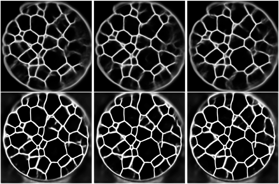
Figure 9. First row: Output of the trained 2D U-Net for three different consecutive CT slices (from left to right). Second row: Output of the trained multichannel U-Net for predicting the grain boundaries of the consecutive slices considered in the first row.

As of now the procedures described above do not provide a grain-wise segmentation. More precisely, the outputs of the U-Net architectures are 3D images with voxel values in the interval (0, 1). Therefore, the network predictions must be binarized in order to localize the grain boundaries, which, however, do not necessarily enclose grains completely. Therefore, additional image processing steps must be carried out in order to obtain a full segmentation of individual grains.

To that end, we binarize the grain boundary predictions (Figure 10A) of the networks ${\widehat{L}}_t$ with a manually determined global threshold followed by morphological closing (Figure 10B). The binarization is followed by a marker-based watershed transformation (Figure 10C), which is performed on the (inverted) Euclidean distance transform of the binary images. In order to reduce oversegmentation in the image obtained by the watershed transformation, a final postprocessing step is carried out in which adjacent regions are merged if the overlap between one region and the convex hull of the neighbor is too large (Figure 10D). For more details on the marker selection procedure for the watershed transformation or the postprocessing step we refer the reader to Spettl et al. (2015).

FIGURE 10

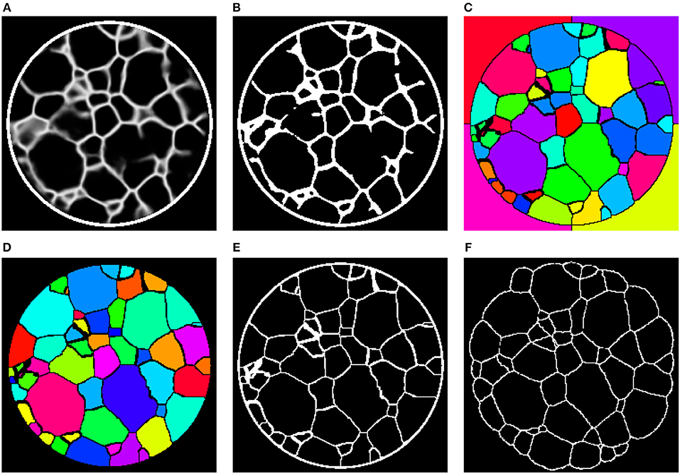
Figure 10. (A) 2D slice through the 3D image ${\widehat{L}}_t$ obtained by preprocessing with the 3D U-Net. (B) Binarization of ${\widehat{L}}_t$ after applying a global threshold, followed by morphological closing. (C) Initial grain-wise segmentation obtained by a marker-based watershed segmentation. (D) Final segmentation after postprocessing. (E) Grain boundaries extracted from the segmentation in (D). (F) Grain boundaries obtained by 3DXRD microscopy.

In order to quantitatively compare segmentations of the CT images C₀, …, C₆ obtained by the 3D U-Net, 2D U-Net and multichannel U-Net followed by the postprocessing steps described above with segmentations derived from the 3DXRD measurements, we first match grains among these segmentations. More precisely, each grain $G_{\mathrm{\text{XRD}}}\subset {ℝ}^3$ observed in a segmentation obtained by 3DXRD microscopy is assigned to a grain $G_{\mathrm{\text{seg}}}\subset {ℝ}^3$ in the corresponding segmentation of the CT image data. We formulated this as a linear assignment problem (Burkard et al., 2012), which minimizes the sum of the volumes of the symmetric differences of matched grains

$\begin{array}{ll}{\nu }_3(G_{\text{XRD}}\Delta G_{\text{seg}})={\nu }_3(G_{\text{XRD}}\setminus G_{\text{seg}})+{\nu }_3(G_{\text{seg}}\setminus G_{\text{XRD}}),& (4)\end{array}$

where ν₃(·) denotes the volume and G_XRDΔG_seg is the symmetric difference given by

$\begin{array}{ll}{G}_{\text{XRD}}\Delta G_{\text{seg}}=\left(G_{\text{XRD}}\setminus G_{\text{seg}}\right)\cup \left(G_{\text{seg}}\setminus G_{\text{XRD}}\right).& (5)\end{array}$

Thus, we will be able to quantitatively compare pairs of matched grains (G_XRD, G_seg) which, in turn, allows a comparison of the presented methods.

3.3. Results

Even though the CNNs described in section 3.2 do not provide grain-wise segmentation of CT data, they can significantly enhance CT images such that conventional image-processing techniques can be readily used to obtain a grain-wise segmentation. By following the approach described in Spettl et al. (2015), we obtained grain-wise segmentations of the considered data set, despite its rather indistinct grain boundaries. A visual comparison between grain boundaries extracted from the segmentation utilizing a 3D U-Net and the true grain boundaries obtained by 3DXRD microscopy indicates that the segmentation is reasonably good, with some oversegmented grains remaining, see Figures 10E,F. A more quantitative comparison becomes available by the grain matching procedure described in section 3.2, i.e., we will compute quantities to measure how much grains segmented from CT deviate from matched grains observed in the ground truth data. More precisely, we determine for pairs of matched grains the relative errors r_V in grain volume given by

$\begin{array}{ll}{r}_V=\frac{|{\nu }_3(G_{\text{XRD}})-{\nu }_3(G_{\text{seg}})|}{{\nu }_3(G_{\text{XRD}})}.& (6)\end{array}$

Also, we computed errors r_c in grain barycenter location normalized by the volume-equivalent diameter of the grain G_XRD. These values are given by

$\begin{array}{ll}{r}_c=\frac{\Vert c(G_{\text{XRD}})-c(G_{\text{seg}})\Vert }{\sqrt[3]{\frac{6}{\pi }{\nu }_3(G_{\text{XRD}}})},& (7)\end{array}$

where ||·|| denotes the Euclidean norm and c(G_XRD), c(G_seg) are the barycenters of the grains G_XRD and G_seg, respectively. Figure 11 visualizes the quartiles of these relative errors in grain characteristics for the segmentation procedures based on the trained 3D U-Net, 2D U-Net and multichannel U-Net. For reference, we also included results obtained by the conventional segmentation procedure without applying neural networks, which was conceptualized for grain boundaries with good visibility and is described in Spettl et al. (2015). These results indicate that the segmentation procedures based on the U-Net architecture perform better then the conventional method. Among the machine learning approaches, the slice-by-slice approach with the 2D U-Net performs worst with a median value for r_V of 0.37. This could be explained by the discontinuities of grain boundary predictions for consecutive slices, see Figure 9. By enhancing the slice-by-slice approach with the multichannel U-Net, we achieve a significant drop of this error down to 0.21. The segmentation approach based on the 3D U-Net performs best with a median error of 0.14, because it is able to learn 3D features for characterizing the grain boundary network embedded in the volumetric data.

FIGURE 11

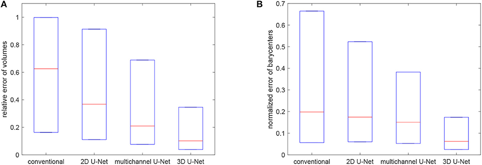
Figure 11. Boxplots visualizing the quartiles of errors of volumes (A) and barycenters (B) for the considered segmentation techniques.

Kernel density estimations (Botev et al., 2010) of the relative errors for the 3D U-Net approach are visualized in Figures 12A,B (blue curves). Furthermore, Figures 12C,D depict these densities for each of the seven observed time steps t = 0, …, 6. Note that, as expected, the errors show a tendency to grow with increasing time step. In order to analyze possible edge effects, i.e., a reduced segmentation quality for grains located at the boundary of the cylindrical sampling window, we computed error densities only for grains located in the interior of the sampling window, see Figures 12A,B. The plots (red curves) indicate that, indeed, the segmentation procedure based on the 3D U-Net works better for interior grains. This effect can be explained by the information that is missing for grains that are cut off by the boundary of the sampling window.

FIGURE 12

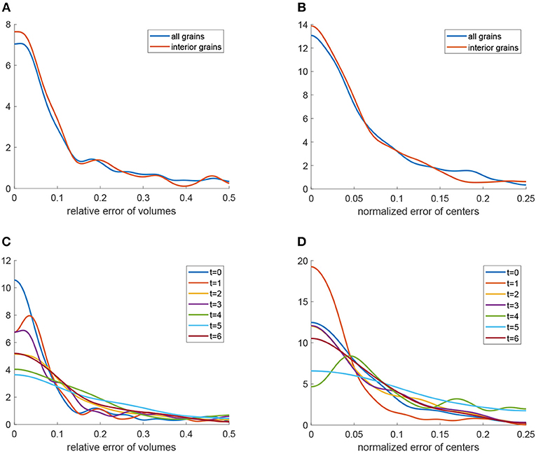
Figure 12. Quantitative analysis of the segmentation procedure based on the 3D U-Net: (A) Kernel density estimation (blue) of relative errors in grain volume. The red curve is the density of relative errors in volume under the condition that the grain is completely visible in the cylindrical sampling window. (B) Kernel density estimation (blue) of normalized errors in grain barycenter location. The red curve is the density of the normalized error in barycenter location under the condition that the grain is completely visible in the cylindrical sampling window. (C) Kernel density estimation of relative errors in grain volume obtained by the segmentation procedure for each measurement step t = 0, …, 6. (D) Kernel density estimation of normalized errors in grain barycenter location obtained by the segmentation procedure for each measurement step t = 0, …, 6.

3.4. Discussion

Although our procedures based on preprocessing with CNNs followed by conventional image processing do not lead to perfect grain segmentations, see Figure 12, especially the method utilizing the 3D U-Net delivers relatively good results when considering the nature of the available CT data. Furthermore, the neural network is able to reduce local artifacts, like liquid inclusions in the grain interiors, which cause small areas of high contrast far from grain boundaries, see Figure 8 (first row). Yet, we warn that the predictions of the trained U-Net are prone to error when there are large-scale image artifacts in the input images, as illustrated in Figure 13. One possible way to reduce the effect of such artifacts is to consider a modified architecture of the 3D U-Net, with larger kernels or more pooling layers, such that even larger features can be considered.

FIGURE 13

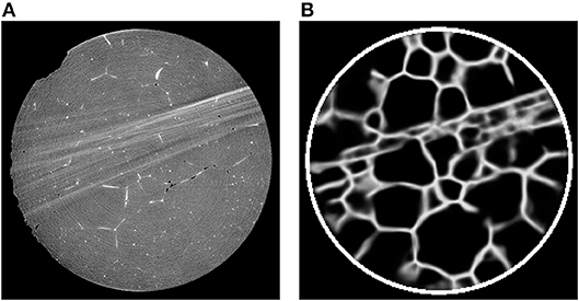
Figure 13. (A) 2D cross-section of a CT image containing reconstruction artifacts and (B) the corresponding prediction of the 3D U-Net.

Nevertheless, without the machine learning approach, i.e., the preprocessing provided by the 3D U-Net, the segmentation of CT data for later measurement time steps with poorly visible grain boundaries is a complex and time-consuming image processing problem. Still, in the presented procedure, conventional image processing, i.e., binarization and the watershed transform, was necessary to obtain a grainwise segmentation of the considered data. Thus, the segmentation techniques considered in sections 2 and 3 show the flexibility of combining the watershed transform with machine learning techniques either for pre- or postprocessing image data for the purpose of segmenting tomographic image data of functional materials.

Note that, in the 3D U-Net approach, there are some machine learning techniques that could have been adopted to further reduce the need for some of the subsequent image processing steps. For example, the binarization step could be incorporated into the network by using the Heaviside step function as an activation function in the output layer. Morphological operations, like the closing operation utilized in the procedure above, could be implemented by additional convolutional layers with non-trainable kernels followed by thresholding. In this way, the necessary postprocessing steps will be considered during the training procedure of the 3D U-Net. Alternatively, by describing a segmentation with an affinity graph on the voxel grid, it is possible to obtain segmented images as the final output of CNNs, see Turaga et al. (2010). Note that such approaches require cost functions which allow a quantitative comparison between segmentations, see e.g., Briggman et al. (2009) and Liebscher et al. (2015). Furthermore, we point out that there are techniques for obtaining a grain-wise segmentation by fitting mathematical tessellation models to tomographic image data using Bayesian statistics and a Markov chain Monte Carlo approach, see Chiu et al. (2013). In our case, such techniques could be applied directly to tomographic or even to enhanced grain boundary images obtained by the 3D U-Net.

Moreover, we note still another possible application of machine learning methods for the analysis of CT image data. In many applications, “ground truth” measurements are destructive, which means that they can be carried out only for the final time step of a sequence of measurements. This limits the available training data for machine learning techniques.

We simulated such a scenario with our data by using solely the CT image C₆ and the 3DXRD data L₆ of the last measured time step to train an additional 3D U-Net. Analogously to the procedure described in section 3.2, this network was applied to the entire series of CT measurements. The resulting grain boundary predictions were then segmented using the same image processing steps as described in section 3.2. Figure 14 indicates that the relative errors of grain volumes are comparable to the errors made when considering every time step during training, see Figure 12. This result suggests that a “ground truth” measurement of only the final time step would suffice for training in our scenario. Similarly, machine learning approaches might be interesting for the segmentation and analysis of time-resolved CT data in various applications in which “ground truth” measurements cannot be made during experiments, but only afterwards, in a destructive or time-consuming manner.

FIGURE 14

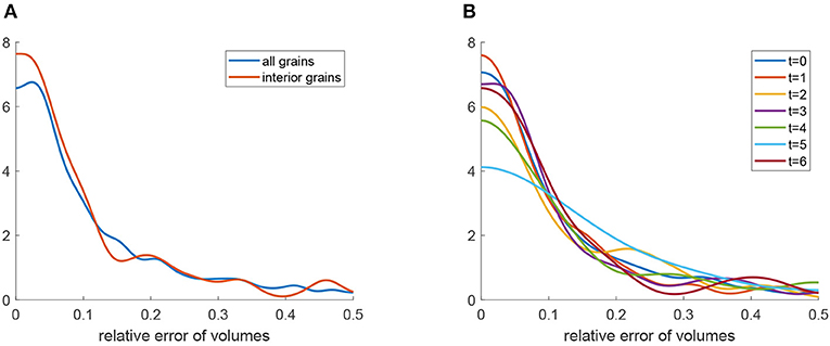
Figure 14. Segmentation results obtained by a 3D U-Net that was trained only with CT/3DXRD data from time step t = 6. (A) Kernel density estimation (blue) of relative errors in grain volume. The red curve is the density of relative errors in volume under the condition that the grain is completely visible in the cylindrical sampling window. (B) Kernel density estimation of relative errors in grain volume obtained by the segmentation procedure for each time step t = 0, …, 6.

4. Conclusions

We gave a short overview of some applications in the field of materials science in which we successfully combined methods of statistical learning, including random forests, feedforward and convolutional neural networks with conventional image processing techniques for segmentation, classification and object detection tasks. More precisely, the methods of sections 2 and 3 utilize machine learning as either a pre- or postprocessing step for the watershed transform to achieve phase-, particle- or grain-wise segmentations of tomographic image data from various functional materials—showing how flexible the approach of combining the watershed transform with methods from machine learning is. In particular, we presented such an approach for segmenting CT image data of an Al-5 wt.% Cu alloy with very low volume fraction of liquid between grains. In total, we considered seven CT measurements of the sample, between which were interspersed Ostwald ripening steps. Especially at later times, the aggregation of liquid leads to a decrease in contrast of the image data, i.e., grain boundaries become less distinct in the image data, which makes segmentation by conventional image processing techniques quite difficult and unreliable. Therefore, we employed matching grain boundary images—which had been extracted from the same sample by means of 3DXRD microscopy—as “ground truth” information for training various CNNs: a 2D U-Net which can be applied slice-by-slice to entire image stacks, a multichannel 2D U-Net which considers multiple slices at once for grain boundary prediction in a planar section of the image stack and, finally, a 3D U-Net which was trained with volumetric cutouts at a lower resolution. After the training procedure, the U-Nets were able to enhance the contrast at grain boundaries in the CT data. Especially, the 3D U-Net successfully predicted the locations of many grain boundaries that were either missing from the image data or poorly visible. This shows that machine learning methods can facilitate difficult image processing tasks, provided that “ground truth” data is available, e.g., data obtained via additional measurements or manual image labeling. Since the images output by the convolutional neural networks were not themselves grain-wise segmentations, we applied conventional image processing algorithms to the outputs to obtain full segmentations at each considered time step and for each presented method. These were compared quantitatively with “ground truth” segmentations extracted from 3DXRD measurements. The resulting relative errors in grain volume and locations of grain centers of mass indicated that the machine learning-based segmentation procedures worked reasonably well, particularly for grains that were not cut off by the boundary of the observation window. Finally, we trained an additional 3D U-Net only with CT and 3DXRD data obtained during the final time step. This simulated the common scenario in which a “ground truth” measurement can be performed only at the very end of an experiment. The 3D U-Net trained in this manner was applied as before to the entire CT data set, followed by conventional image processing steps, yielding grain segmentations. Quantitative comparison of the latter to segmentations derived from 3DXRD data indicated that the approach produced good results. Even though a trained neural network does not make 3DXRD measurements obsolete, the procedure presented here can potentially reduce the amount of 3DXRD beam time that is needed for accurate segmentation and microstructural analysis. Likewise, we believe that a similar approach might be particularly beneficial whenever nondestructive CT measurements can be carried out in situ, but “ground truth” information can be acquired only by a destructive measurement technique.

Author Contributions

OF, MN, LP, and MWe reviewed previous results on machine learning for segmentation of image data. Tomographic image data of the AlCu specimen has been provided by MWa and CK. The network training, segmentation and analysis of AlCu CT image data was performed by OF. All authors discussed the results and contributed to writing of the manuscript. CK and VS designed the research.

Conflict of Interest Statement

The authors declare that the research was conducted in the absence of any commercial or financial relationships that could be construed as a potential conflict of interest.

Acknowledgments

The financial support of the German Research Foundation (DFG) for funding this research project (SCHM997/23-1) is gratefully acknowledged. The authors thank Murat Cankaya for the processing of image data. In addition, the authors are grateful to the Japan Synchrotron Radiation Research Institute for the allotment of beam time on beamline BL20XU of SPring-8 (Proposal 2015A1580).

References

Beare, R., and Lehmann, G. (2006). The watershed transform in ITK-discussion and new developments. Insight J. 92, 1–24. Available online at: http://hdl.handle.net/1926/202

Google Scholar

Beucher, S., and Lantuéjoul, C. (1979). “Use of watersheds in contour detection,” in International Workshop on Image Processing, Real-Time Edge and Motion Detection/Estimation, Vol. 132 (Rennes).

Google Scholar

Bhandari, Y., Sarkar, S., Groeber, M., Uchic, M., Dimiduk, D., and Ghosh, S. (2007). 3D polycrystalline microstructure reconstruction from FIB generated serial sections for FE analysis. Comput. Mater. Sci. 41, 222–235. doi: 10.1016/j.commatsci.2007.04.007

CrossRef Full Text | Google Scholar

Bishop, C. M. (2006). Pattern Recognition and Machine Learning. New York, NY: Springer.

Google Scholar

Botev, Z. I., Grotowski, J. F., and Kroese, D. P. (2010). Kernel density estimation via diffusion. Ann. Stat. 38, 2916–2957. doi: 10.1214/10-AOS799

CrossRef Full Text | Google Scholar

Briggman, K., Denk, W., Seung, S., Helmstaedter, M. N., and Turaga, S. C. (2009). “Maximin affinity learning of image segmentation,” in Advances in Neural Information Processing Systems, eds Y. Bengio, D. Schuurmans, J. Lafferty, C. Williams, and A. Culotta (Vancouver, BC: NIPS), 1865–1873.

Google Scholar

Burkard, R., Dell'Amico, M., and Martello, S. (2012). Assignment Problems. Philadelphia, PA: SIAM.

Google Scholar

Chiu, S. N., Stoyan, D., Kendall, W. S., and Mecke, J. (2013). Stochastic Geometry and Its Applications. Chichester: J. Wiley & Sons.

Google Scholar

Chollet, F. (2015). Keras. Available online at: https://keras.io

Google Scholar

Çiçek, Ö., Abdulkadir, A., Lienkamp, S. S., Brox, T., and Ronneberger, O. (2016). “3D U-Net: learning dense volumetric segmentation from sparse annotation,” in International Conference on Medical Image Computing and Computer-Assisted Intervention, eds S. Ourselin, L. Joskowicz, M. R. Sabuncu, G. Unal, and W. Wells (Cham: Springer), 424–432.

Google Scholar

Dake, J. M., Oddershede, J., Sørensen, H. O., Werz, T., Shatto, J. C., Uesugi, K., et al. (2016). Direct observation of grain rotations during coarsening of a semisolid Al-Cu alloy. Proc. Natl. Acad. Sci. U.S.A. 113, E5998–E6006. doi: 10.1073/pnas.1602293113

PubMed Abstract | CrossRef Full Text | Google Scholar

Falk, T., Mai, D., Bensch, R., Çiçek, Ö., Abdulkadir, A., Marrakchi, Y., et al. (2019). U-Net: deep learning for cell counting, detection, and morphometry. Nat. Methods 16:67. doi: 10.1038/s41592-018-0261-2

CrossRef Full Text | Google Scholar

Feinauer, J., Brereton, T., Spettl, A., Weber, M., Manke, I., and Schmidt, V. (2015a). Stochastic 3D modeling of the microstructure of lithium-ion battery anodes via Gaussian random fields on the sphere. Comput. Mater. Sci. 109, 137–146. doi: 10.1016/j.commatsci.2015.06.025

CrossRef Full Text | Google Scholar

Feinauer, J., Spettl, A., Manke, I., Strege, S., Kwade, A., Pott, A., et al. (2015b). Structural characterization of particle systems using spherical harmonics. Mater. Characterizat. 106, 123–133. doi: 10.1016/j.matchar.2015.05.023

CrossRef Full Text | Google Scholar

Finegan, D. P., Scheel, M., Robinson, J. B., Tjaden, B., Michiel, M. D., Hinds, G., et al. (2016). Investigating lithium-ion battery materials during overcharge-induced thermal runaway: an operando and multi-scale X-ray CT study. Phys. Chem. Chem. Phys. 18, 30912–30919. doi: 10.1039/C6CP04251A

PubMed Abstract | CrossRef Full Text | Google Scholar

Furat, O., Leißner, T., Ditscherlein, R., Šedivý, O., Weber, M., Bachmann, K., et al. (2018). Description of ore particles from X-ray microtomography (XMT) images, supported by scanning electron microscope (SEM)-based image analysis. Microsc. Microanal. 24, 461–470. doi: 10.1017/S1431927618015076

PubMed Abstract | CrossRef Full Text | Google Scholar

Geder, J., Hoster, H. E., Jossen, A., Garche, J., and Yu, D. Y. W. (2014). Impact of active material surface area on thermal stability of LiCoO2 cathode. J. Power Sour. 257, 286–292. doi: 10.1016/j.jpowsour.2014.01.116

CrossRef Full Text | Google Scholar

Girshick, R. (2015). “Fast R-CNN,” in Proceedings of the IEEE International Conference on Computer Vision (Santiago: IEEE), 1440–1448.

Google Scholar

Girshick, R., Donahue, J., Darrell, T., and Malik, J. (2014). “Rich feature hierarchies for accurate object detection and semantic segmentation,” in Proceedings of the IEEE Conference on Computer Vision and Pattern Recognition (Columbus, OH), 580–587. doi: 10.1109/CVPR.2014.81

CrossRef Full Text | Google Scholar

Glorot, X., Bordes, A., and Bengio, Y. (2011). “Deep sparse rectifier neural networks,” in Proceedings of the Fourteenth International Conference on Artificial Intelligence and Statistics, Vol. 15. eds G. Gordon, D. Dunson, and M. Dudík (Fort Lauderdale, FL: JMLR W&CP), 315–323.

Google Scholar

Goodfellow, I., Bengio, Y., Courville, A., and Bengio, Y. (2016). Deep Learning. Vol. 1. Cambridge: MIT Press.

Google Scholar

Hastie, T., Tibshirani, R., and Friedman, J. (2009). The Elements of Statistical Learning, 2nd Edn. New York, NY: Springer.

Google Scholar

He, K., Gkioxari, G., Dollár, P., and Girshick, R. (2017). “Mask R-CNN,” in Proceedings of the IEEE International Conference on Computer Vision (Venice: IEEE), 2980–2988.

PubMed Abstract | Google Scholar

James, G., Witten, D., Hastie, T., and Tibshirani, R. (2013). An Introduction to Statistical Learning. New York, NY: Springer.

Google Scholar

Jiang, J., and Dahn, J. R. (2004). Effects of particle size and electrolyte salt on the thermal stability of Li0.5CoO2. Electrochim. Acta 49, 2661–2666. doi: 10.1016/j.electacta.2004.02.017

CrossRef Full Text | Google Scholar

Kingma, D. P., and Ba, J. L. (2015). “Adam: a method for stochastic optimization,” in Proceedings of 3rd International Conference on Learning Representations, eds D. Suthers, K. Verbert, E. Duval, and X. Ochoa (San Diego, CA).

Google Scholar

Kuchler, K., Prifling, B., Schmidt, D., Markötter, H., Manke, I., Bernthaler, T., et al. (2018). Analysis of the 3D microstructure of experimental cathode films for lithium-ion batteries under increasing compaction. J. Microsc. 272, 96–110. doi: 10.1111/jmi.12749

PubMed Abstract | CrossRef Full Text | Google Scholar

Liebscher, A., Jeulin, D., and Lantuéjoul, C. (2015). Stereological reconstruction of polycrystalline materials. J. Microsc. 258, 190–199. doi: 10.1111/jmi.12232

PubMed Abstract | CrossRef Full Text | Google Scholar

Massalski, T. (1996). Binary Alloy Phase Diagrams, 3rd Edn. Vol. 1. Materials Park, OH: ASM International.

Google Scholar

Meyer, F. (1994). Topographic distance and watershed lines. Sig. Process. 38, 113–125. doi: 10.1016/0165-1684(94)90060-4

CrossRef Full Text | Google Scholar

Naylor, P., Lae, M., Reyal, F., and Walter, T. (2017). “Nuclei segmentation in histopathology images using deep neural networks,” in 2017 IEEE 14th International Symposium on Biomedical Imaging (ISBI 2017) (Melbourne, VIC: IEEE), 933–936.

Google Scholar

Neumann, M., Cabiscol, R., Osenberg, M., Markötter, H., Manke, I., Finke, J.-H., et al. (2019). Characterization of the 3D microstructure of ibuprofen tablets by means of synchrotron tomography. J. Microsc. 274, 102–113. doi: 10.1111/jmi.12789

PubMed Abstract | CrossRef Full Text | Google Scholar

Nocedal, J., and Wright, S. J. (2006). Numerical Optimization, 2nd Edn. Springer Series in Operations Research and Financial Engineering. New York, NY: Springer.

Google Scholar

Nunez-Iglesias, J., Kennedy, R., Parag, T., Shi, J., and Chklovskii, D. B. (2013). Machine learning of hierarchical clustering to segment 2D and 3D images. PLoS ONE 8:e71715. doi: 10.1371/journal.pone.0071715

PubMed Abstract | CrossRef Full Text | Google Scholar

Petrich, L., Westhoff, D., Feinauer, J., Finegan, D. P., Daemi, S. R., Shearing, P. R., et al. (2017). Crack detection in lithium-ion cells using machine learning. Comput. Mater. Sci. 136, 297–305. doi: 10.1016/j.commatsci.2017.05.012

CrossRef Full Text | Google Scholar

Poulsen, H. F. (2012). An introduction to three-dimensional X-ray diffraction microscopy. J. Appl. Crystallogr. 45, 1084–1097. doi: 10.1107/S0021889812039143

CrossRef Full Text | Google Scholar

Ren, S., He, K., Girshick, R., and Sun, J. (2017). Faster R-CNN: towards real-time object detection with region proposal networks. IEEE Trans. Patt. Anal. Mach. Intell. 39, 1137–1149. doi: 10.1109/TPAMI.2016.2577031

PubMed Abstract | CrossRef Full Text | Google Scholar

Roerdink, J. B., and Meijster, A. (2000). The watershed transform: definitions, algorithms and parallelization strategies. Fundamenta Informaticae 41, 187–228.

Google Scholar

Ronneberger, O., Fischer, P., and Brox, T. (2015). “U-Net: convolutional networks for biomedical image segmentation,” in International Conference on Medical Image Computing and Computer-Assisted Intervention, eds N. Navab, J. Hornegger, W. Wells, and A. Frangi (Cham: Springer), 234–241.

Google Scholar

Rowenhorst, D., Gupta, A., Feng, C., and Spanos, G. (2006a). 3D crystallographic and morphological analysis of coarse martensite: combining EBSD and serial sectioning. Scripta Mater. 55, 11–16. doi: 10.1016/j.scriptamat.2005.12.061

CrossRef Full Text | Google Scholar

Rowenhorst, D., Kuang, J., Thornton, K., and Voorhees, P. (2006b). Three-dimensional analysis of particle coarsening in high volume fraction solid-liquid mixtures. Acta Mater. 54, 2027–2039. doi: 10.1016/j.actamat.2005.12.038

CrossRef Full Text | Google Scholar

Schmidt, S. (2014). Grainspotter: a fast and robust polycrystalline indexing algorithm. J. Appl. Crystallogr. 47, 276–284. doi: 10.1107/S1600576713030185

CrossRef Full Text | Google Scholar

Schmidt, S., Olsen, U., Poulsen, H., Soerensen, H., Lauridsen, E., Margulies, L., et al. (2008). Direct observation of 3-D grain growth in Al-0.1% Mn. Scripta Mater. 59, 491–494. doi: 10.1016/j.scriptamat.2008.04.049

CrossRef Full Text | Google Scholar

Soille, P. (2013). Morphological Image Analysis: Principles and Applications. Berlin: Springer.

Google Scholar

Sommer, C., Straehle, C., Koethe, U., and Hamprecht, F. A. (2011). “Ilastik: interactive learning and segmentation toolkit,” in IEEE International Symposium on Biomedical Imaging: From Nano to Macro (Chicago, IL: IEEE), 230–233.

Google Scholar

Spettl, A., Wimmer, R., Werz, T., Heinze, M., Odenbach, S., Krill, C. III., et al. (2015). Stochastic 3D modeling of Ostwald ripening at ultra-high volume fractions of the coarsening phase. Model. Simulat. Mater. Sci. Eng. 23:065001. doi: 10.1088/0965-0393/23/6/065001

CrossRef Full Text | Google Scholar

Stenzel, O., Pecho, O., Holzer, L., Neumann, M., and Schmidt, V. (2017). Big data for microstructure-property relationships: a case study of predicting effective conductivities. AIChE J. 63, 4224–4232. doi: 10.1002/aic.15757

CrossRef Full Text | Google Scholar

Turaga, S. C., Murray, J. F., Jain, V., Roth, F., Helmstaedter, M., Briggman, K., et al. (2010). Convolutional networks can learn to generate affinity graphs for image segmentation. Neural Comput. 22, 511–538. doi: 10.1162/neco.2009.10-08-881

PubMed Abstract | CrossRef Full Text | Google Scholar

Werz, T., Baumann, M., Wolfram, U., and Krill III, C. (2014). Particle tracking during Ostwald ripening using time-resolved laboratory X-ray microtomography. Mater. Characterizat. 90, 185–195. doi: 10.1016/j.matchar.2014.01.022

CrossRef Full Text | Google Scholar

Xue, D., Xue, D., Yuan, R., Zhou, Y., Balachandran, P. V., Ding, X., et al. (2017). An informatics approach to transformation temperatures of NiTi-based shape memory alloys. Acta Mater. 125, 532–541. doi: 10.1016/j.actamat.2016.12.009

CrossRef Full Text | Google Scholar