 Brandon D. Snow
 Dustin D. Doty
 Oliver K. Johnson
94% of researchers rate our articles as excellent or good
Learn more about the work of our research integrity team to safeguard the quality of each article we publish.
Find out more
ORIGINAL RESEARCH article
Front. Mater., 31 May 2019
Sec. Computational Materials Science
Volume 6 - 2019 | https://doi.org/10.3389/fmats.2019.00120
This article is part of the Research TopicMachine Learning and Data Mining in Materials ScienceView all 16 articles
Grain boundaries (GBs) have a significant influence on the properties of crystalline materials. Machine learning approaches present an attractive route to develop atomic structure-property models for GBs because of the complexity of their structure. However, the application of such techniques requires an appropriate descriptor of the atomic structure. Unfortunately, common crystal structure identification techniques cannot be applied to characterize the structure of the vast majority of GB atoms (50–98% are classified as “other”). This suggests a critical need for atomic structure descriptors capable of identifying arbitrary atomic environments. In this work we present a simple procedure that facilitates the identification of arbitrary atomic structures present in GBs. We apply this approach to characterize the atomic structure of the 388 GBs from the Olmsted data set (Olmsted et al., 2009). We show how this approach facilitates visualization of GB atomic structures in a way that reveals important structural information. We test the recently proposed hypothesis that Σ3 GBs contain facets of the GBs that form the corners of the corresponding GB plane fundamental zone. Finally, we briefly demonstrate how the structure descriptors resulting from our approach can be used as inputs to machine learning approaches for the development of atomic structure-property models for GBs.
Grain boundaries (GBs) play an important role for many material properties, such as hydrogen embrittlement (Bechtle et al., 2009), creep (Gertsman and Tangri, 1997; Watanabe et al., 2009), corrosion resistance (Shimada et al., 2002; Tan et al., 2008), and conductivity (Zhang et al., 2006). While the structure of GBs is most often characterized experimentally by their five macroscopic crystallographic degrees of freedom (Ashby et al., 1978), it is the atomic structure that fundamentally governs their properties (Katritzky and Fara, 2005). Atomistic simulation has been used to investigate the atomic structure of GBs and how it correlates with their observed properties (Zhang et al., 2009). However, the atomic structure of GBs is much more complicated than their crystallographic structure and traditional crystal identification descriptors are not designed to classify the structure of the vast majority of atoms present at GBs. As an example, we analyzed the 388 GBs constructed by Olmsted et al. (2009) using common crystal structure identification methods: bond-angle analysis (BAA) (Ackland and Jones, 2006), common neighbor analysis (CNA) (Faken and Jónsson, 1994), and polyhedral template matching (PTM) (Larsen et al., 2016). Table 1 provides the percentage of the GB atoms that were unclassified (i.e., classified as “other”/unknown structures) by each technique across all 388 GBs and across the subset of 41 Σ3 GBs. The fact that 50–98% of the GB atoms remain unclassified, makes it difficult to identify atomic structure-property relationships for GBs, and suggests a critical need for new techniques that can describe the complex atomic structure of GBs.
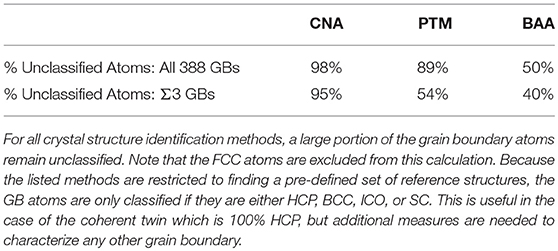
Table 1. Comparison of characterization methods applied to the Olmsted GB data set (Olmsted et al., 2009).
Due to the complex and high-dimensional nature of GB atomic structures, machine learning and related statistical approaches provide an attractive route for the development of atomic structure-property models. However, the inability to resolve atomic structure within GBs complicates such an effort because the effect of distinct atomic environments cannot be extracted if these environments cannot be distinguished. If it were possible to fully characterize the atomic structure of GBs, dimensionality reduction techniques such as feature selection (e.g., decision trees) and feature transformation (e.g., principle component analysis) could be applied to identify the atomic environments that govern properties of interest. Labeled data from simulations could then be provided to train supervised machine learning algorithms, and predictive models could be developed that would significantly expand our understanding of atomic structure-property relations for GBs.
As demonstrated above, common crystal structure identification techniques are insufficient for this task. Consequently, several authors have developed methods to identify arbitrary non-crystalline atomic structures for applications such as developing interatomic potentials (Bartók et al., 2013), analyzing colloidal crystallization (Reinhart et al., 2017), and characterizing grain boundaries (Banadaki and Patala, 2017; Rosenbrock et al., 2017; Priedeman et al., 2018). A brief summary of their work is given in section 2. While these methods are effective, they are also significantly more complex than simple crystal structure identification techniques that are in common use. The major contribution of the present work is to bridge this gap.
By employing a simple version of common neighbor analysis (CNA) and leveraging information that is already available—but which is normally discarded—we develop an approach that (i) can characterize arbitrary atomic environments, while also being both (ii) simple to implement, and (iii) built upon a descriptor that is already familiar to the atomistic modeling community. We demonstrate that, in spite of its simplicity, it can be employed for predictive purposes as part of a machine learning strategy to develop GB structure-property models. We anticipate that the simplicity and effectiveness of this approach will facilitate the development of predictive structure-property models for GBs as well as other applications that involve lower symmetry atomic structures such as those present in metallic glasses.
There has been great interest in characterizing atomic structures recently and over the last decade and several reviews are available in the literature (Stukowski, 2012; Priedeman, 2018), so only a brief description is given here.
Common methods used to identify crystalline structures include the centrosymmetry parameter (Kelchner et al., 1998), common neighbor analysis (CNA) (Faken and Jónsson, 1994), polyhedral template matching (PTM) (Larsen et al., 2016), and Voronoi cell analysis methods (Bernal, 1959; Rahman, 1966; Bernal and Finney, 1967; Finney, 1970; Hsu and Rahman, 1979; Sheng et al., 2006; Lazar et al., 2015).
The centrosymmetry parameter is a measure of the distance to an atom's n nearest neighbors to determine whether or not an atom is within a bulk crystal or a defect. CNA, PTM, and Voronoi analysis methods all classify the atomic structure of an atom by comparison of its local environment to a library of known structures, usually face-centered cubic (FCC), hexagonal close-packed (HCP), body-centered cubic (BCC), icosahedral (ICO), and, for some of these methods, simple cubic (SC).
These methods provide valuable tools for identifying the location, and in some cases the types, of defects present in an atomistic model. However, as with all tools (including those that we present in this paper), each method has certain drawbacks and limitations. The main disadvantages of the centrosymmetry parameter are that the number of neighbors, n, is a user-defined parameter, and the centrosymmetry parameter doesn't give any insight into what the local structure is if it is part of a defect. While some of the limitations of CNA have been reduced by the introduction of an adaptive cutoff radius (Stukowski, 2012), the method is typically just used to determine whether an atom belongs to one of a small set of predetermined environments. PTM uses a more robust Voronoi method to identify neighbors, but it too relies on comparison with a small library of known environments. Voronoi analysis generally characterizes local environments by the number of faces with a particular number of edges, but this approach fails to distinguish between some common environments (FCC and HCP) (Bernal, 1959; Rahman, 1966; Bernal and Finney, 1967; Finney, 1970; Hsu and Rahman, 1979; Sheng et al., 2006). The recently developed Voronoi Topology (VoroTop) technique (Lazar et al., 2015) uses planar graph representations to address this issue by including information about the arrangement of the faces, but requires a large database of nearly degenerate variants of the known Voronoi cells to compare against, since small atomic displacements can significantly affect the Voronoi cell topology. As with the other crystal structure identification methods, the VoroTop technique has primarily employed a small library of known structures. Additional environments can be added to these libraries, but this must be done manually.
To adequately analyze the local atomic structure of defects, such as GBs, a method is needed that can classify atoms without a priori knowledge of the structures present (i.e., without reliance on a small precomputed list of known structures). Several recent publications have presented methods to identify arbitrary local environments (Bartók et al., 2013; Banadaki and Patala, 2017; Reinhart et al., 2017; Rosenbrock et al., 2017; Priedeman et al., 2018), and a brief description of each is given here.
Bartók et al. (2013) developed an atomic structure descriptor based on the superposition of Gaussian kernels centered at atomic positions, referred to as the SOAP kernel/descriptor. SOAP is unique in that it is a continuous descriptor (making it robust against small changes in atomic positions) unlike most other descriptors that are discrete in nature. SOAP has recently been applied to characterize GBs by Rosenbrock et al. (2017) and Priedeman et al. (2018).
Banadaki and Patala (2017) presented the polyhedral unit model, which compares the neighborhood around voids in atomic structures (at which vertices in the Voronoi tessellation are centered) against an exhaustive library of configurations of close-packed spheres for up to 12 spheres. A benefit of the polyhedral unit model is that an RMSD value can be calculated to quantify how close of a match particular structures are to their reference structures, but the resulting polyhedra are centered on a void as opposed to an atom which is the more common representation of an atomic environment.
Reinhart et al. (2017) developed an algorithm called Neighborhood Graph Analysis (NGA), which implemented CNA with an adaptive cutoff radius to produce CNA signatures for arbitrary environments present in colloidal crystallization simulations. The adaptive cutoff however, produces an asymmetric neighborhood graph (i.e., atom B may be a neighbor to atom A, but that does not imply atom A will be in the neighborhood set of atom B) which can artificially increase the number of unique environments (i.e., there is an over-partitioning of the configuration space). This is compensated for by employing a machine learning algorithm to determine relationships between otherwise discrete signatures and consolidate similar environments that have different signatures. Reinhart et. al subsequently developed a modified version of their original algorithm, which they call the “fast NGA” (fNGA) algorithm (Reinhart and Panagiotopoulos, 2018), which defines neighbors using a Delaunay triangulation (similar to PTM), and which uses graphlets to dramatically reduce the computational cost of the consolidation step. The present work can be seen as a simplified version of Reinhart's original approach.
While all of these methods are effective at classifying non-crystalline atomic environments, they are complex and in some cases computationally expensive. In this paper we present a comparatively simple alternative based on CNA to identify arbitrary local environments without the use of a predetermined library of structures. Because of its simplicity and the fact that it only requires some minor post-processing (code provided in Supplementary Material) of traditional CNA data that is already ubiquitously available in existing software packages, our approach can be easily adopted. While our method, like others, suffers from over-partitioning of the space of unique atomic environments, we show that it is, nevertheless, possible to gain insight into important structure-property relationships. We demonstrate the usefulness of this technique by characterizing the unique atomic environments (UAEs) present in the 388 GBs of the Olmsted data set (Olmsted et al., 2009). We also test the recent hypothesis (Banadaki and Patala, 2016) that the structures of Σ3 GBs may decompose into facets of the GBs occupying the corners of the corresponding GB plane fundamental zone (FZ). Finally, we give a brief example of how the UAEs identified using our approach might serve as inputs to machine learning strategies for the development of atomic structure-property models for GBs.
In the traditional CNA method, a set of three indices (j, k, l) is defined, which describes the topology of the graph formed by the nearest neighbor atoms (see Figure 1). The three indices are computed for each neighboring atom to define their relationship to the central atom. The first index j enumerates the number of shared nearest neighbors (e.g., in Figure 1 the four light purple atoms are nearest neighbors of both the central atom and the dark purple atom, so for the dark purple atom j = 4). The index k enumerates the number of bonds between shared nearest neighbors (e.g., in Figure 1 there are two dashed purple lines indicating two distinct bonds between shared nearest neighbors, so for the dark purple atom k = 2). Finally, the index l enumerates the number of bonds in the longest bond-chain formed by shared neighbors (e.g., in Figure 1 the dashed purple lines do not share an atom, so the longest bond-chain between shared nearest neighbors is 1, giving l = 1 for the dark purple atom). CNA indices are calculated for each atom pair. The local environment (i.e., “atomic structure”) of a particular atom is then defined by the set of CNA indices of all of its nearest neighbors. As has been done in prior literature (Stukowski, 2012; Reinhart et al., 2017), we refer to this as an atom's CNA signature to distinguish it from the atom's CNA indices. For example, the CNA signature of an atom whose local structure corresponds to an FCC lattice would be denoted {12 × (4, 2, 1)}, indicating that it possesses 12 nearest neighbors, each with CNA indices of (4, 2, 1). An atom with a less symmetric local environment, such as one belonging to a GB might have a CNA signature of {2 × (3, 1, 1), 3 × (4, 2, 1), 2 × (4, 2, 2), 2 × (4, 3, 3), } {1 × (4, 4, 4), 2 × (5, 4, 4)}, indicating a total of twelve nearest neighbors, but which have different CNA indices.
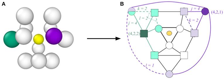
Figure 1. Illustration of the process for determining CNA indices and the CNA signature, concept inspired by Reinhart et al. (2017). In (A) an atom is shown (central yellow atom, which has been reduced in size for visual clarity) together with its nearest neighbors. The corresponding graph representation is provided in (B). The light colored symbols represent the nearest neighbors shared with the central atom (four for the purple neighbor and four for the green neighbor). Solid lines represent bonds between neighbors of the central atom, while dashed lines represent bonds between shared neighbors (two for both the purple and green neighbors). For the purple neighbor the shared bonds (dashed lines) are not connected, so k = 1, but for the green neighbor the shared bonds are connected so k = 2. Because of the symmetry of this graph, there are six neighbors with the same indices (4, 2, 1) as the purple atom (represented by circles) and six with the same indices (4, 2, 2) as the green (represented by squares). Consequently the CNA signature for the central atom is {6 × (4, 2, 1), 6 × (4, 2, 2)}, which represents an HCP atomic environment.
We note that neighbors can be identified using various methods, the primary ones being a fixed cutoff radius or an adaptive cutoff (Stukowski, 2012; Reinhart et al., 2017). In this work we chose to use a fixed cutoff of 3.5Å (which falls between the first and second nearest neighbors for the FCC lattice, see Figure 3A). The fixed cutoff was chosen both because of its simplicity and because it resulted in fewer unique signatures than the adaptive methods (2205 vs. 3716) for the structures that we analyzed.
Once the CNA signature of every atom has been computed, atomic structures are identified by comparison with the CNA signatures of a predefined library of known structures, typically limited to FCC, HCP, BCC, and ICO. In standard usage, any atom whose CNA signature does not match that of one of the predefined structural templates remains unclassified and is labeled as “other.” This is sufficient to identify the location of defects because “other” atoms typically are found at defects. However, it is generally insufficient to resolve the structure of those defects. Because GBs consist of mostly “other” atoms, their internal atomic structure cannot typically be resolved. Furthermore, if two GBs both contain all “other” atoms, it is difficult to distinguish between them.
To address this issue, we note that the information necessary to distinguish “other” atoms from one another is already available and encoded in their respective CNA signatures, it is just typically ignored in standard practice. To exploit this information one must simply identify all of the unique CNA signatures; these define distinct atomic structure classes; in some sense this list constitutes an extended structure library. Atoms are then classified using this extended structure library. However, it is constructed at the time of analysis and is compatible with arbitrary atomic structures (one does not need to know what structures they are looking for a priori). Furthermore, the “other” category is entirely eliminated as all atoms are classified and belong to one of the UAEs that were identified.
To extract the complete CNA signatures for each atom in the structures that we analyzed, there are built-in functions that can be run as part of a pipeline in the Open Visualization Tool (OVITO) (Stukowski, 2010), and an example python script is available in the online OVITO documentation. We modified this script for our particular application, and we provide our modified version in the accompanying Supplementary Material. Once extracted, the unique CNA signatures were then identified in MATLAB and each was assigned a unique numerical class ID (we also provide this code in the Supplementary Material), which was subsequently imported into OVITO as a custom particle property, allowing for color-coding and visualization.
We applied the fully-leveraged CNA approach to characterize all of the atoms in the 388 GBs from the Olmsted data set (Olmsted et al., 2009), which contains atomic structures for a total of 388 GBs in Al with variation across all five crystallographic degrees of freedom, including 41 Σ3 GBs. Here we present the results of that analysis. The vast majority of the atoms belong to the grain interiors and are FCC, and could be easily characterized by existing methods. We, therefore, focus on the GB atoms, which are generally classified as “other”/unidentified structures by reference structure based techniques. We define an atom as belonging to the GB if at least one of the nearest neighbors is not FCC. This results in all of the non-FCC atoms, as well as many FCC atoms inside or adjacent to the GB being identified with it (for some tilt GBs, if the dislocation spacing is sufficiently large there will be FCC atoms in the GB plane, that are entirely surrounded by other FCC atoms, which would not be counted as GB atoms by this definition.). Using this definition, there are a total of 462,955 GB atoms, out of a total of 11,922,451 atoms contained in the Olmsted data set (the non-GB atoms belong to the bulk crystal and are all FCC). While some GBs properly contain FCC atoms in their interior (e.g., low-angle GBs have FCC atoms between dislocations), the focus of this work is on characterizing non-FCC atoms. Consequently, we will present our results in two ways: (i) relative to all 462,955 GB atoms (FCC and non-FCC), and (ii) relative to only the non-FCC GB atoms (of which there are 227,401).
Figure 2A shows the distribution of GB atomic environments across all 388 GBs for the fully-leveraged CNA approach. This shows that out of the nearly 500,000 GB atoms (across all 388 GBs), there are 2205 unique CNA signatures. However, noting the log-scale in the y-axis, only 448 signatures are needed to account for approximately 90% of the non-FCC GB atoms (see Figure 2B), and only 167 are needed if the GB atoms with FCC structure are included1. While this still represents a non-negligible number of unique environments, it is a considerable reduction in dimensionality for a general set of grain boundaries, which would otherwise require a total of at least 682, 203 parameters to describe the atomic configurations (3 parameters for each atom Rosenbrock et al., 2017).
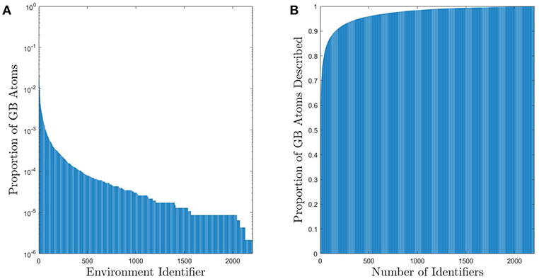
Figure 2. (A) Histogram of UAEs found in the 388 Omlsted GBs. Note that this is on a log scale and there are approximately 5 × 105 GB atoms. (B) Cumulative sum of the proportion of atoms that can be described using a given number of UAEs. Approximately 90% of the non-FCC GB atoms can be described by one of the 448 most prevalent UAEs (only 167 UAEs are required if the GB atoms with FCC structure are included).
We note that, using an alternative spatially continuous descriptor, smooth overlap of atomic positions (SOAP) (Bartók et al., 2013), Rosenbrock et al. initially found 800,000 UAEs for the same 388 GBs in Ni, using a neighborhood cutoff distance of 5Å (Rosenbrock et al., 2017). In the SOAP method, as well as other methods such as PTM, a similarity measure is employed, enabling two structures that differ by only a small perturbation to still be classified as the same environment, which is one way to correct for the overpartitioning phenomenon. After using a similarity metric within a machine learning framework the original 800,000 UAEs were consolidated to only 145 distinct UAEs. We note that, as with any similarity based consolidation approach, the resulting number of unique environments depends on the user specified similarity threshold.
The simple approach to UAE identification embodied in the fully-leveraged CNA does not employ a similarity threshold, so it is expected that the UAE space will be over-partitioned. This manifests itself in the relatively long-tailed distribution of UAEs in Figure 2, which are produced by small deviations in atomic position that cause a single environment to produce multiple CNA signatures (i.e., UAEs that are not frequently observed are most likely slightly distorted versions of other UAEs). The underlying cause of this phenomenon is the difficulty in unambiguously defining atomic neighbors in non-crystalline regions. To illustrate this, compare the radial distribution function (RDF) for bulk FCC with that of a grain boundary, as shown in Figure 3. The clear separation of the first and second peaks—corresponding to the first and second nearest neighbors, respectively—in the RDF of the FCC lattice (Figure 3A) facilitates the selection of an appropriate neighbor cutoff radius. However, as expected, the RDF for the grain boundary atoms (Figure 3B) does not show a clear separation between first and second neighbors, making CNA sensitive to small perturbations of atomic position and changes in the cutoff radius. This also means that the number of UAEs identified by the fully-leveraged CNA approach of the present work depends on the user chosen cutoff radius. This challenge exists for any method that attempts to characterize GB atoms, because there is no clear choice as to which atoms should be included in the neighborhood, and the resulting structures are likely to over-partition the UAE space.
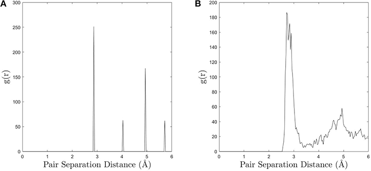
Figure 3. (A) The radial distribution function (RDF) for an FCC lattice calculated in OVITO and (B) the RDF for the grain boundary atoms (a GB was used as a representative example).The distinct peaks in the bulk FCC make it easy to choose an appropriate cutoff distance for neighbor identification, however the more continuous nature of the GB RDF causes CNA to be more sensitive to small perturbations in atomic position and changes in the cutoff.
As mentioned earlier, work has been done by Reinhart et al. (2017) to establish a machine learning approach to identify environments that have similar structure but different CNA signatures and combine them into a single environment (i.e., clustering in the UAE space). This effectively implements a similarity metric for CNA, and was successful in its application to surfaces of colloidal crystals. However, this process is computationally expensive and does not result in a single universal partitioning of the UAE space, so the repartitioning would need to be recalculated (or at least updated) for every new data set to be characterized. In spite of the overpartitioning that results from the simple fully-leveraged CNA approach, and in the absence of environment consolidation, we find that useful analysis can still be performed to evaluate GB structure-property models as will be described in section 4.3.
For the subset of Σ3 GBs, the number of UAEs is reduced considerably. Figure 4 shows the distribution of atomic environments found in the subset of 41 Σ3 GBs, for which there were only 117 unique CNA signatures. Moreover, the vast majority of the GB atoms (roughly 90%) correspond to one of just 44 UAEs (or only 29 UAEs if GB atoms with FCC structure are included). This kind of dimensionality reduction for descriptions of GB atomic structure may make inference of GB atomic structure-property models significantly more tractable. Furthermore, this information can be used to compare the structural similarity of different GBs as will be discussed in section 4.3.
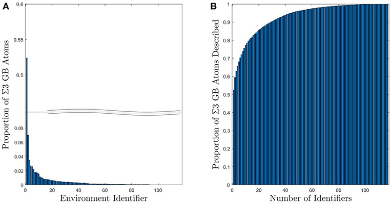
Figure 4. (A) Histogram of UAEs found in Σ3 GBs. The large spike at environment 1 corresponds to the FCC structural type and is due to the inclusion of the first layer of FCC atoms as part of the GB. (B) Cumulative sum of the proportion of Σ3 GB atoms that can be described using a given number of UAEs. Approximately 90% of the Σ3 atoms correspond to one of the 44 most prevalent UAEs.
Without resorting to the more advanced machinery of SOAP or Reinhart's machine learning approach, most analysis of atomic structures relies on the simpler reference structure based crystal structure identification techniques. Because they were designed to identify crystalline regions, and not GBs, 50%−98% of the GB atoms in the Olmsted data set are, unsurprisingly, classified as “other” by the reference structure based techniques, making the atomic structure of these GBs largely opaque to classical analysis. As revealed by our fully-leveraged CNA technique, the fact that only 44 UAEs dominate the Σ3 GBs studied here suggests the possibility of discovering new GB structural information for very little computational effort, and within the familiar CNA framework. We illustrate this through visualization, by coloring GB atoms according to their UAE identifier. As an example, Figures 5A,B provides a rendering of a GB with atoms colored according to standard practice (using the traditional CNA approach). The FCC atoms (in green) are identified, but all of the atoms at the GB are classified as “other”/unidentified environments. In contrast, Figure 5C shows the same GB atoms colored using the atomic environment classes identified by our fully-leveraged CNA technique. It is evident that this GB contains a structured arrangement of atomic environments and is quasi-two dimensional. This new approach reveals structure that was previously unresolvable using the common crystal structure identification techniques, and for far less computational effort than the more advanced techniques.
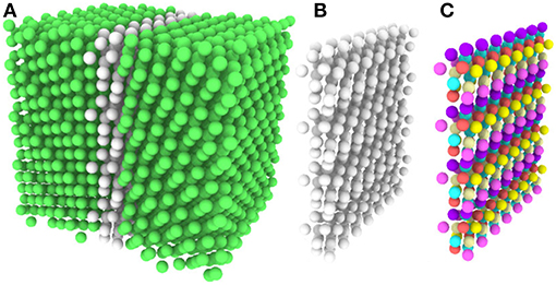
Figure 5. (A) OVITO rendering of a GB, with atoms colored by traditional CNA. Green atoms are FCC, white are “other”. Notice that all of the GB atoms remain unidentified. (B) All FCC atoms removed. (C) Atoms colored by the UAE IDs obtained from our fully-leveraged CNA procedure.
In addition to the ability to easily obtain important structural information for a single GB, coloring each atom according to its local environment facilitates identification of structural similarity among different GBs. In the case of Σ3 GBs, it has been hypothesized that GBs may form facets whose structure corresponds to that of the GBs that occupy the corners of the relevant boundary plane fundamental zone (FZ) (Banadaki and Patala, 2016). However, a test of this hypothesis would require comparison of the atomic structures of various GBs, which would be difficult using reference structure based descriptors that leave nearly all of those atoms unclassified. For example, the top row of Figure 6 shows three different Σ3 GBs that are near each other in the FZ. While terrace-like features are apparent, it is unclear whether these represent facets of the same structure. Using the fully-leveraged CNA procedure, the bottom row of Figure 6 makes it clear that each of these GBs do in fact contain very similar environments, giving some evidence in support of the faceting hypothesis. A more complete analysis of faceting in Σ3 GBs, enabled by the fully-leveraged CNA technique, is provided in section 4.3.
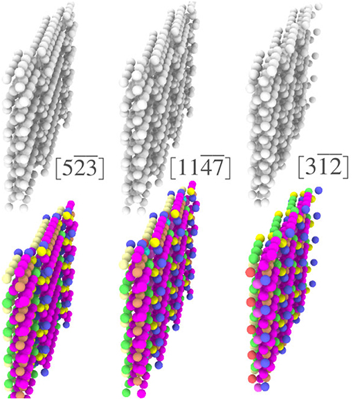
Figure 6. Visualization of three Σ3 GBs (boundary plane is indicated in brackets), (above) with atoms colored using traditional CNA available in OVITO, and (below) colored by the UAEs found during the fully-leverage CNA procedure.
Visualizing a grain boundary in this manner also highlights higher-order defects, or defects inside of other defects (note the dark purple environments that decorate the ledges in Figure 6).
Here we apply the fully-leveraged CNA technique to investigate the relationship between atomic structure and GB properties. As mentioned previously, it was recently hypothesized by Banadaki and Patala (2016) that Σ3 GBs may be composed of facets whose structure corresponds to that of the 3 GBs that define the corners of the Σ3 GB plane FZ. Based on this hypothesis, Banadaki and Patala developed a structure-property model to predict the GB energy of an arbitrary Σ3 GB as a weighted average of the GB energies of the FZ corners. This model showed good agreement with GB energies calculated by MD for many cases. However, the GB structures were never analyzed to test whether the hypothesized structural faceting actually occurred. The fully-leveraged CNA approach presented here provides an opportunity to test this hypothesis.
The total number of UAEs found in each of the GBs that define the corners of the Σ3 GB plane FZ are provided in Table 2. It is notable that the UAEs appearing in each of the corner GBs form disjoint sets. This implies that they are in some sense orthogonal structures, which might at first appear to support the possibility of faceting. However, the total number of environments (117) found across all of the 41 Σ3 GBs is greater than the total number of environments found in the FZ corners (12), and, as shown in Figure 7, these additional environments are not concentrated at ledges between facets, but constitute significant portions of the non-corner GBs.
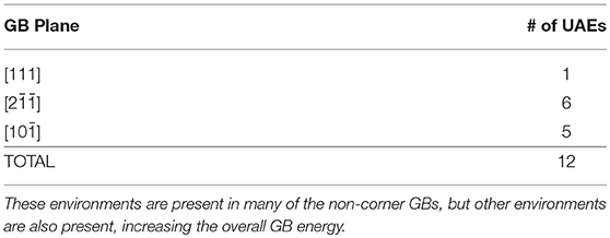
Table 2. Summary of UAEs found in the Σ3 fundamental zone.
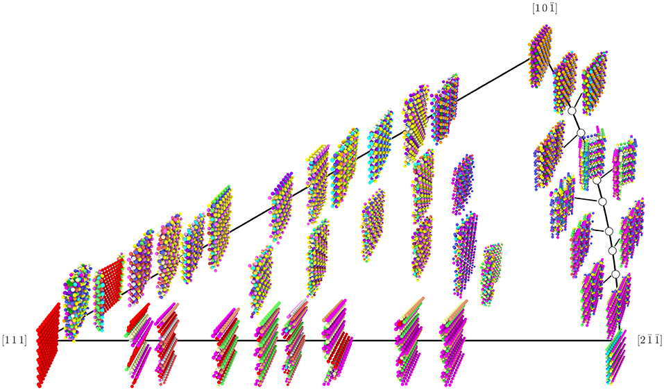
Figure 7. Rendering of the 41 Σ3 GBs from the Olmsted data set, with atoms colored by their UAE ID. Position in the FZ is relative and approximate (exact placement would cause some images to overlap). Colors were selected manually for the most frequently occurring UAEs in an effort to maximize visual differences between atoms of different UAE ID that are near each other; however, some less frequently observed UAEs do share the same color.
Several key observations can be derived from Figure 7. First, there are in fact some regions of the FZ where the GBs are made of facets of the corner GBs. In particular, GBs near the [111] coherent twin (θ = ϕ = 0) show obvious facets whose structure is that of the coherent twin. Also, GBs along the right boundary of the FZ (θ = 90°) show some evidence of faceting (this behavior near the corner was also noted by Banadaki and Patala, 2017), though for many of these GBs the structure of these facets does not correspond to any of the FZ corners. As for the rest of the FZ, there is no clear evidence of faceting for the Olmsted Al GBs. It is important to note, however, that the ability of a GB to facet in an atomistic model may depend on the size of the simulation cell that was employed to construct it (see Race et al., 2014; Humberson and Holm, 2017, for a discussion of the impact of simulation cell size), so that it is possible that if larger simulation cells were used, faceting might be observed more generally. Moreover, it has been shown that there can be many metastable atomic structures for the same GB (Han et al., 2017), some of which have nearly degenerate energies. Thus, it is also possible that there are distinct iso-energetic configurations, or that the atomic structures in this data set may not be the lowest energy configurations, which might otherwise exhibit the hypothesized faceting structure. Indeed, Banadaki and Patala found atomic structures for the Σ3 GBs with considerably lower energies in many cases (Banadaki and Patala, 2016), which may have exhibited faceting more generally, and this may be one explanation for the better fit of the faceting model's energy predictions to their data than to the Olmsted data (see Figure 9). Regardless of whether or not the atomic structures in the Olmsted data set are ground state structures or (at least in some cases) metastable structures, the fully-leveraged CNA approach can be applied to characterize the atomic structure that is present, whatever it happens to be. Furthermore, if ground state structures were available, our fully-leveraged CNA approach would easily identify more general faceting if it were to occur in those structures.
Although structural faceting does not occur generally for the Olmsted atomic structures, relatively smooth trends in the composition of UAEs are observed across the FZ. Figure 8 shows the fraction of atoms in each GB whose atomic environments match those of each of the FZ corners. For all three corners, smooth trends in atomic environment composition are observed along θ = 90° from to (for the corner it is smooth, but not monotonic, see Figure 8B). Smooth trends also occur along ϕ = 0 from [111] to and near the coherent twin. Furthermore, as the crystallographic distance to one of the corner GBs increases, the proportion of atomic environments belonging to that corner decreases. This suggests that in the absence of faceting (which represents a sort of structural segregation behavior) there may be a sort of mixing behavior of atomic environments from each of the FZ corners for these GB structures.
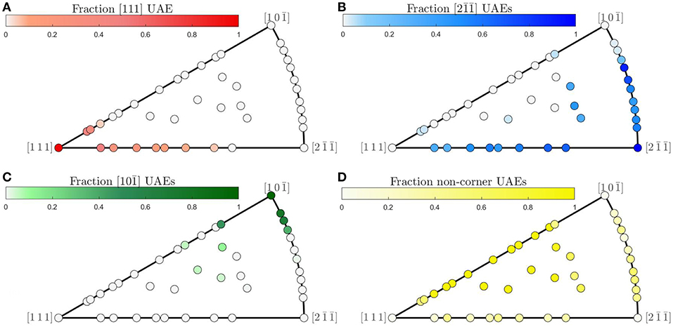
Figure 8. (A–C) Fraction of GB atoms whose local environment belongs to the set of UAEs present in each of the respective corners of the fundamental zone and (D) fraction of environments not present in any of the FZ corners.
Because we do not observe structural faceting generally, it is not surprising that the faceting model does not predict the energies of the Olmsted data set well. However, for some regions of the FZ there are also deviations between the faceting model's predictions and the calculated GB energies for the lower energy atomic structures obtained by Banadaki and Patala. It is notable that where these deviations do occur, they are almost exclusively underpredictions. Our observations here may partially explain this behavior. The faceting model predicts GB energy as a weighted average of the energies of the GBs at the FZ corners, which ignores the energetic contribution of the line defects that will likely exist at the junction of distinct facets, and underpredictions are therefore consistent with this omission. These line defects are likely to be composed of atomic environments that are not present in the FZ corners, and which may have higher cohesive energies. In fact, we find that the non-corner atomic environments have an average cohesive energy2 that is 3.5 × 10⁻²¹ J (0.022 eV) higher than the average for the atomic environments that belong to the FZ corners. This may seem like a small difference, but because many GBs contain a large portion of non-corner environments (a median of 49% of the GB atoms) the cumulative effect can be significant. A rough estimate is illustrative: if 50% of a GB's atoms (e.g., 500 of 1000) are non-corner environments and possess the average non-corner environment cohesive energy (−5.30 × 10⁻¹⁹ J or −3.31 eV) then with a GB area of 1800 Å2 (the average cross-section for an Olmsted simulation cell) the non-corner environments would contribute approximately 0.097 J/m2 to the GB energy, which is similar to the magnitude of the underpredictions shown in Figure 9.
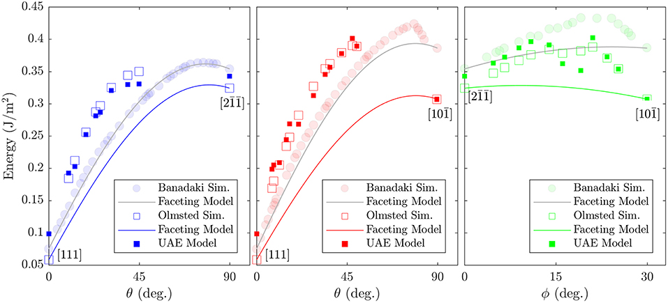
Figure 9. Comparison of calculated GB energies for GBs that lie along the edges of the Σ3 fundamental zone with the predictions of Banadaki and Patala's faceting model (Banadaki and Patala, 2016). Two data sets of calculated GB energies are included: (open squares) those from Olmsted et al. (2009) and (semi-transparent filled circles) those from Banadaki and Patala (2016). The predictions of the UAE model are also included (filled squares), for comparison with the Olmsted simulations (open squares).
This suggests that a model based on atomic environments, might provide improved predictions for GB energy. We note that important work in this area has already been performed by Rosenbrock et. al within the SOAP framework (Rosenbrock et al., 2017). The rigorous development of such a model is beyond the scope of the present work, whose primary objective has been to present a simple atomic structure characterization technique (the fully-leveraged CNA approach) that enables characterization of GB atomic structure that was unresolvable using crystal structure identification approaches. Nevertheless, we provide a simple and brief example of how the resulting UAEs might be incorporated into machine learning or other model development approaches.
We treat the fraction of each UAE as a predictor (independent) variable and the energy of the GB as the response (dependent) variable. This implies a 2205 dimensional space (corresponding to the 2205 UAEs observed across all 388 GBs). We employ PCA to perform feature transformation and selection and find that only 84 principle components (linear combinations of the original variables) are required to explain 95% of the variance in the data. Thus, we have reduced the dimensionality of the problem from 2205 to 84 dimensions. Using these 84 transformed variables, we employ 5-fold cross-validation to train a simple linear regression model. Comparison of the resulting model to the calculated GB energies for all 388 GBs is provided in Figure 10, with the subset of Σ3 GBs highlighted. Comparison of the model predictions to the Olmsted simulations for the subset of Σ3 GBs as a function of boundary plane orientation is also provided in Figure 9 (compare filled vs. open squares). The resulting model predictions agree well with the calculated values, and the model predicts the correct GB energy with less than 10% error for 89.69% of the 388 GBs (and 92.68% of the Σ3 GBs). We note, in particular, the improved predictions of the UAE model across the θ = 90° arc of the FZ from to (the green filled squares agree well with the green open squares in the right panel of Figure 9) as compared to the faceting model (solid green line).
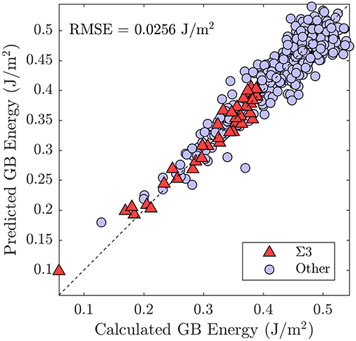
Figure 10. Comparison of the predictions of the model—trained using the UAE fractions as variables—with the true calculated GB energies from the Olmsted data set (Olmsted et al., 2009).
In this work, we have presented an atomic structure characterization technique (the fully-leveraged CNA approach) that (i) can characterize arbitrary atomic environments, while also being both (ii) simple to implement, and (iii) built upon a descriptor that is already familiar to the atomistic modeling community. This enables characterization of GB atomic structure that was previously unresolvable using crystal structure identification techniques, and for lower computational effort than more advanced techniques. We show that it is possible to describe GB atomic structure in terms of the proportion of the unique atomic environments (UAEs) resulting from the use of our method.
We find that a relatively small number of UAEs account for a large proportion of the GB atoms, suggesting the possibility of a significant dimensionality reduction in the description of GB atomic structure. Specifically, we found that to describe 90% of the non-FCC GB atoms present in the 388 GBs of the Olmsted data set, only 448 UAEs (CNA signatures) are required, and for the subset of 41 Σ3 GBs only 44 UAEs are necessary. This dimensionality reduction suggests that these UAEs can act as atomic structure descriptors that might be incorporated into machine learning approaches to develop improved GB structure-property models.
We demonstrated how visualization of the UAEs reveals important GB structural information. As an example, we investigated the possible description of Σ3 GBs as being composed of facets of the GBs occupying the corners of the corresponding boundary plane fundamental zone (FZ). We found that for the Olmsted data set such faceting does occur in certain regions of the FZ, but not generally. Instead, an apparent mixing of atomic environments from the GBs defining the FZ corners was observed, together with the appearance of numerous environments not present in the FZ corners. These observations are consistent with the good agreement of the faceting model with calculated GB energies for some regions of the FZ, as well as the observed underprediction in other regions.
Finally, we provided a brief example to illustrate how the UAE fractions can be used as GB atomic structure descriptors that can serve as input to machine learning approaches for the development of GB atomic structure-property models.
The datasets for this study will not be made publicly available because some data has been used with permission. All other data is available upon request to the corresponding author.
OJ designed the project and trained the final model. BS and DD developed all of the analysis codes and performed the calculations and analysis. All authors contributed to preparation of the manuscript.
This work has been supported by the Department of Mechanical Engineering at Brigham Young University.
The authors declare that the research was conducted in the absence of any commercial or financial relationships that could be construed as a potential conflict of interest.
We are grateful to Dr. Eric R. Homer and Dr. Srikanth Patala for fruitful discussions, and to Dr. David Olmsted for permission to use the Al GB structures.
The Supplementary Material for this article can be found online at: https://www.frontiersin.org/articles/10.3389/fmats.2019.00120/full#supplementary-material
1. ^Including the GB atoms that have FCC structure only adds one UAE, but because GB atoms that possess FCC structure make up a significant percentage of the total GB atoms, fewer UAEs are required to represent 90% of the total GB atoms.
2. ^We computed the cohesive energies in LAMMPS (Plimpton, 1995) using the same potential that Olmsted et. al used to produce these Al structures (the Ercolessi & Adams potential for aluminum Liu et al., 2004).
Ackland, G. J., and Jones, A. P. (2006). Applications of local crystal structure measures in experiment and simulation. Phys. Rev. B 73:054104. doi: 10.1103/PhysRevB.73.054104
Ashby, M. F., Spaepen, F., and Williams, S. (1978). The structure of grain boundaries described as a packing of polyhedra. Acta Metal. 26, 1647–1663. doi: 10.1016/0001-6160(78)90075-5
Banadaki, A. D., and Patala, S. (2016). A simple faceting model for the interfacial and cleavage energies of Σ3 grain boundaries in the complete boundary plane orientation space. Comput. Mater. Sci. 112, 147–160. doi: 10.1016/j.commatsci.2015.09.062
Banadaki, A. D., and Patala, S. (2017). A three-dimensional polyhedral unit model for grain boundary structure in fcc metals. npj Comput. Mater. 3:13. doi: 10.1038/s41524-017-0016-0
Bartók, A. P., Kondor, R., and Csányi, G. (2013). On representing chemical environments. Phys. Rev. B Condens. Matter Mater. Phys. 87, 1–16. doi: 10.1103/PhysRevB.87.184115
Bechtle, S., Kumar, M., Somerday, B., Launey, M., and Ritchie, R. (2009). Grain-boundary engineering markedly reduces susceptibility to intergranular hydrogen embrittlement in metallic materials. Acta Mater. 57, 4148–4157. doi: 10.1016/J.ACTAMAT.2009.05.012
Bernal, J. (1959). A geometrical approach to the structure of liquids. Nature 183. 141–147. doi: 10.1038/183141a0
Bernal, J. D., and Finney, J. L. (1967). Random close-packed hard-sphere model. ii. geometry of random packing of hard spheres. Discuss. Faraday Soc. 43, 62–69. doi: 10.1039/DF9674300062
Faken, D., and Jónsson, H. (1994). Systematic analysis of local atomic structure combined with 3D computer graphics. Comput. Mater. Sci. 2, 279–286. doi: 10.1016/0927-0256(94)90109-0
Finney, J. L. (1970). Random packings and the structure of simple liquids. I. The geometry of random close packing. Proc. R. Soc. Lond. Ser. A Math. Phys. Sci. 319, 479–493. doi: 10.1098/rspa.1970.0189
Gertsman, V., and Tangri, K. (1997). Modelling of intergranular damage propagation. Acta Mater. 45, 4107–4116. doi: 10.1016/S1359-6454(97)00083-9
Han, J., Vitek, V., and Srolovitz, D. J. (2017). The grain-boundary structural unit model redux. Acta Mater. 133, 186–199. doi: 10.1016/J.ACTAMAT.2017.05.002
Hsu, C. S., and Rahman, A. (1979). Interaction potentials and their effect on crystal nucleation and symmetry. J. Chem. Phys. 71, 4974–4986. doi: 10.1063/1.438311
Humberson, J., and Holm, E. A. (2017). Anti-thermal mobility in the Σ3 [111] 60 {11 8 5} grain boundary in nickel: mechanism and computational considerations. Scripta Mater. 130, 1–6. doi: 10.1016/J.SCRIPTAMAT.2016.10.032
Katritzky, A. R., and Fara, D. C. (2005). How chemical structure determines physical, chemical, and technological properties: an overview illustrating the potential of quantitative structure property relationships for fuels science. Energy Fuels 19, 922–935. doi: 10.1021/ef040033q
Kelchner, C. L., Plimpton, S. J., and Hamilton, J. C. (1998). Dislocation nucleation and defect structure during surface indentation. Phys. Rev. B 58, 11085–11088. doi: 10.1103/PhysRevB.58.11085
Larsen, P. M., Schmidt, S., and Schiøtz, J. (2016). Robust structural identification via polyhedral template matching. Model. Simul. Mater. Sci. Eng. 24:055007. doi: 10.1088/0965-0393/24/5/055007
Lazar, E. A., Han, J., and Srolovitz, D. J. (2015). A topological framework for local structure analysis in condensed matter. Proc. Natl. Acad. Sci. U.S.A. 112, E5769–E5776. doi: 10.1073/pnas.1505788112
Liu, X., Ercolessi, F., and Adams, J. (2004). Aluminium interatomic potential from density functional theory calculations with improved stacking fault energy. Model. Simul. Mater. Sci. Eng. 12, 665–670. doi: 10.1088/0965-0393/12/4/007
Olmsted, D. L., Foiles, S. M., and Holm, E. A. (2009). Survey of computed grain boundary properties in face-centered cubic metals: I. Grain boundary energy. Acta Mater. 57, 3694–3703. doi: 10.1016/j.actamat.2009.04.007
Plimpton, S. (1995). Fast parallel algorithms for short-range molecular dynamics. J. Comput. Phys. 117, 1–19. doi: 10.1006/jcph.1995.1039
Priedeman, J. L. (2018). Quantifying Grain Boundary Atomic Structures Using the Smooth Overlap of Atomic Positions (Master's thesis). Brigham Young University, USA.
Priedeman, J. L., Rosenbrock, C. W., Johnson, O. K., and Homer, E. R. (2018). Quantifying and connecting atomic and crystallographic grain boundary structure using local environment representation and dimensionality reduction techniques. Acta Mater. 161, 431–443. doi: 10.1016/j.actamat.2018.09.011
Race, C. P., Von Pezold, J., and Neugebauer, J. (2014). Role of the mesoscale in migration kinetics of flat grain boundaries. Phys. Rev. B 89:214110. doi: 10.1103/PhysRevB.89.214110
Rahman, A. (1966). Liquid structure and self-diffusion. J. Chem. Phys. 45, 2585–2592. doi: 10.1063/1.1727978
Reinhart, W. F., Long, A. W., Howard, M. P., Ferguson, A. L., and Panagiotopoulos, A. Z. (2017). Machine learning for autonomous crystal structure identification. Soft Matter 13, 4733–4745. doi: 10.1039/C7SM00957G
Reinhart, W. F., and Panagiotopoulos, A. Z. (2018). Automated crystal characterization with a fast neighborhood graph analysis method. Soft Matter 14, 6083–6089. doi: 10.1039/C8SM00960K
Rosenbrock, C. W., Homer, E. R., Csányi, G., and Hart, G. L. W. (2017). Discovering the building blocks of atomic systems using machine learning: application to grain boundaries. npj Comput. Mater. 3:29. doi: 10.1038/s41524-017-0027-x
Sheng, H., Luo, W., Alamgir, F. M., Bai, J. M., and Ma, E. P. (2006). Atomic packing and short-to-medium-range order in metallic glasses. Nature 439, 419–425. doi: 10.1038/nature04421
Shimada, M., Kokawa, H., Wang, Z., Sato, Y., and Karibe, I. (2002). Optimization of grain boundary character distribution for intergranular corrosion resistant 304 stainless steel by twin-induced grain boundary engineering. Acta Mater. 50, 2331–2341. doi: 10.1016/S1359-6454(02)00064-2
Stukowski, A. (2010). Visualization and analysis of atomistic simulation data with OVITO–the Open Visualization Tool. Model. Simul. Mater. Sci. Eng. 18:015012. doi: 10.1088/0965-0393/18/1/015012
Stukowski, A. (2012). Structure identification methods for atomistic simulations of crystalline materials. Model. Simul. Mater. Sci. Eng. 20:045021. doi: 10.1088/0965-0393/20/4/045021
Tan, L., Sridharan, K., Allen, T., Nanstad, R., and McClintock, D. (2008). Microstructure tailoring for property improvements by grain boundary engineering. J. Nucl. Mater. 374, 270–280. doi: 10.1016/J.JNUCMAT.2007.08.015
Watanabe, T., Tsurekawa, S., Zhao, X., and Zuo, L. (2009). “The coming of grain boundary engineering in the 21st century ,” in Microstructure and Texture in Steels (London: Springer), 43–82.
Zhang, H., Srolovitz, D. J., Douglas, J. F., and Warren, J. A. (2009). Grain boundaries exhibit the dynamics of glass-forming liquids. Proc. Natl. Acad. Sci. U.S.A. 106, 7735–7740. doi: 10.1073/pnas.0900227106
Keywords: grain boundary, machine learning, atomic structure identification, common neighbor analysis, faceting
Citation: Snow BD, Doty DD and Johnson OK (2019) A Simple Approach to Atomic Structure Characterization for Machine Learning of Grain Boundary Structure-Property Models. Front. Mater. 6:120. doi: 10.3389/fmats.2019.00120
Received: 03 March 2019; Accepted: 09 May 2019;
Published: 31 May 2019.
Edited by:
Norbert Huber, Helmholtz Centre for Materials and Coastal Research (HZG), GermanyReviewed by:
Peter Larsen, Massachusetts Institute of Technology, United StatesCopyright © 2019 Snow, Doty and Johnson. This is an open-access article distributed under the terms of the Creative Commons Attribution License (CC BY). The use, distribution or reproduction in other forums is permitted, provided the original author(s) and the copyright owner(s) are credited and that the original publication in this journal is cited, in accordance with accepted academic practice. No use, distribution or reproduction is permitted which does not comply with these terms.
*Correspondence: Oliver K. Johnson, b2pvaG5zb25AYnl1LmVkdQ==
Disclaimer: All claims expressed in this article are solely those of the authors and do not necessarily represent those of their affiliated organizations, or those of the publisher, the editors and the reviewers. Any product that may be evaluated in this article or claim that may be made by its manufacturer is not guaranteed or endorsed by the publisher.
Research integrity at Frontiers
Learn more about the work of our research integrity team to safeguard the quality of each article we publish.