Impacts of temporal growth variability on fisheries stock assessment in changing oceans: a case study of Eastern Atlantic skipjack

Climate change affects the somatic growth of many important fish species targeted by fisheries worldwide, yet the explicit incorporation of climate-driven temporal growth variation in assessment remains limited for most fisheries stocks. In this study, we use Eastern Atlantic skipjack (Katsuwonus pelamis) as a case study to explore the effects of misspecifying temporal growth variation driven by sea surface temperature on stock assessments, highlighting the potential risks associated with neglecting temporal growth variation under both historical and future climate conditions. Misspecification of temporal growth variation in stock assessment models is found to introduce bias in the estimated quantities of interest in informing fisheries management, regardless of whether the “true” growth varies with time. Our findings indicate that the estimated quantities of management interest, in particular, the SSB-associated quantities (e.g., stock depletion) are more sensitive to the inclusion of time-varying L_inf than to time-varying K. We emphasize the importance of incorporating temporal variation in fish asymptotic length into the stock assessments of Eastern Atlantic skipjack under the effects of future climate change. Consequently, integrating environmental data into stock assessment is necessary for climate-adaptive stock assessment and fisheries management.

1 Introduction

Fish somatic growth has been widely recognized to be influenced by climate-induced environmental variations (Thresher et al., 2007; Rountrey et al., 2014; Wang et al., 2020), particularly water temperature, which affects developmental biology processes of fish such as muscle differentiation and organogenesis (Jobling, 2002), as well as metabolism-regulating mechanisms (Boltaña et al., 2017; Heather et al., 2018; Gamperl et al., 2020). Meta-analyses have shown that warming generally negatively affects fish growth at both global and local scales (Huang et al., 2021). Furthermore, climate-driven fish growth may have long-lasting impacts on recruitment success (Jonsson and Jonsson, 2009) and ultimately lead to alternations in population productivity (Harley et al., 2006; Thorson et al., 2015; Britten et al., 2017), even in fish species considered less sensitive to climate change (Rountrey et al., 2014).

In fisheries stock assessments, fish growth is typically modeled as constant over time, i.e., based on the temporally-stationary hypothesis (Lee et al., 2018). However, growth can vary both across and within species over time (see Appendix A of Thorson et al., 2015 for more details), which highlights the inherent plasticity of fish growth (Brett, 1979; Weatherley, 1990). Climate change and its uncertainties pose unprecedented challenges to fisheries management, which seeks fishery sustainability. Neglecting time-varying growth may lead to substantial biases in assessment results and weaken the effectiveness of management grounded in scientific advice (Punt et al., 2013; Merino et al., 2019). Management quantities are found to be overestimated if fish growth is misspecified, particularly in the estimates of current biomass relative to the unfished biomass, leading to an overestimation of stock status (Stawitz et al., 2019). The estimates of spawning stock biomass in an integrated assessment model may exhibit significant bias when the declining trend of growth parameters is not considered (Kuriyama et al., 2016). Therefore, accurately identifying and quantifying the climate-driven fish growth in stock assessments is critical for providing the best available information for fisheries management.

Recognizing the advantages of incorporating time-varying growth over adhering to the ‘constant growth’ paradigm (Lorenzen, 2016; Maunder and Watters, 2003), the internal modeling of growth variability has been more widely accepted in recent stock assessment platforms. Stock Synthesis (SS3) allows variation in growth over time by introducing parameter deviations or linking them with environmental factors (Methot and Wetzel, 2013). Another common approach is using empirical weight-at-age (EWAA) information to account for growth variation, as seen in the Woods Hole Assessment Model (WHAM, Stock and Miller, 2021). WHAM has been extended to link climate variables to growth (Correa et al., 2023), with process error variance being estimated by integrating random effects and maximizing marginal likelihood, in line with the ‘best practices’ for handling process error (Punt, 2023). Despite these advancements, incorporating climate-driven temporal growth variation is not common in most oceanic species stock assessments. For highly migratory species like tunas, it remains challenging to quantify the interactions between fish life history processes and environmental factors over short-term observations and explicitly incorporate these relationships into stock assessments. Alternative hypotheses of these relationships may be developed through the accumulated observations, however, most often fail to stand the test of time (Sinclair and Crawford, 2005). Additionally, such practices have been a compromise for methodological consistency in scientific evaluation (Hilborn, 2012).

The tropical Atlantic warming serves as the ‘engine’ of tropical-wide climate change (Li et al., 2016) and has the potential to propagate globally. Climate change impacts tropical fisheries not only for local fishery industries but also extends to the extratropical regions through the ‘tele-coupling’ effect (Lam et al., 2020). Tropical tunas’ longline catches decreased in tropical waters and increased in subtropical waters during 1965-2011, which was attributed to a poleward shift under climate change rather than a change in fishing strategies (Monllor-Hurtado et al., 2017; Erauskin-Extramiana et al., 2019). Skipjack (Katsuwonus pelamis), a tropical tuna species with high landings and economic values, grows rapidly and is highly responsive to environmental temperatures. For instance, the otolith daily increment analysis indicated temperature-induced geographic differences in Pacific skipjack growth during its early life (Ashida et al., 2018). Specifically, the mean growth rate until 10 days after hatching was positively correlated with mean sea surface temperature, suggesting temperature-related growth variability of juvenile skipjack in the western and central Pacific Ocean would occur during the larval stage (Ashida et al., 2018).

Recent Atlantic skipjack stock assessments have adopted time-invariant life history parameters such as growth in modeling population dynamics, which may introduce additional uncertainties in its management. Here, we used Eastern Atlantic skipjack as a case study to explore the implications of misspecifying temporal variation in growth parameters K and L_inf (Von Bertalanffy, 1938) in stock assessment through simulation modeling. Sea surface temperature (SST) was factored into the population dynamics as a proxy for climate change. Both historical and future climate conditions were considered to examine the temporal impact of climate-driven water warming on fish growth and stock assessment. This study intends to explore three issues: (a) how model performance is affected by including temporal growth variation in the assessment when the “true” growth is time-invariant; (b) how model performance is affected by misspecifying temporal growth variation when the “true” growth (K or L_inf) varies over time; and (c) how model performance is affected by including only time-varying K or L_inf, or considering both as time-invariant, when the “true” growth (K and L_inf) varies over time. Our goal is to illustrate the consequences of misspecification of growth parameters on quantities of management interest and highlight the risks of neglecting temporal growth variation in fisheries stock assessments under historical and future climate conditions.

2 Materials and methods

2.1 Overview

The Von Bertalanffy growth function (Equation 1) (Von Bertalanffy, 1938) is the growth model used in the Eastern Atlantic skipjack stock assessment (ICCAT, 2022). It is written as:

$\begin{array}{ll}{L}_t=L_{inf}(1-e^{-K(t-t_0)})& (1)\end{array}$

where L_t is the length-at-age t, L_inf is the asymptotic average maximum body size, K is the intrinsic growth rate coefficient (year^-1), and t₀ is a constant representing the hypothetical age at which the fish species has zero length.

In this study, a simulation framework was constructed using the statistical age-structured population model, Stock Synthesis (SS3, Methot and Wetzel, 2013), which serves as both the operating model (OM) and the estimation model (EM). The OM was used to simulate “true” population dynamics and generate data series, including catch, abundance index and length composition, which were used as input data for the EM. The simulation framework consists of the following steps: (a) simulating a 100-year time series of population dynamics with recruitment process error using the OM, with fishing periods commencing from year 30; (b) applying the EM to data series generated from the OM with observation error; and (c) comparing the estimates of key quantities of management interest with the “true” values defined by the OM. Each scenario underwent 200 iterations to ensure the comparability of results (Johnson et al., 2015). The framework was implemented using the ‘ss3sim’ R package (Anderson et al., 2014), a widely used tool in fisheries stock assessment simulation testing.

Given that the “true” growth is unknown, three assumptions are made in this study: (a) assuming the “true” growth is time-invariant; (b) assuming the “true” growth rate K is time-varying while the “true” asymptotic length L_inf is time-invariant, and vice versa, and (c) assuming both the “true” growth rate K and asymptotic length L_inf are time-varying.

To compare and illustrate the potential impact of sea surface temperature on fish growth across different temporal contexts under climate change, this study resembled both historical and future climate conditions. These climate conditions are assumed to be independent, rather than treating the future as a projection of the historical one. Additionally, within the future climate condition, two climate scenarios were considered: the Shared Socioeconomic Pathway 5-8.5 (SSP5-8.5), which represents a fossil fuel-intensive scenario, and the Shared Socioeconomic Pathway 1-2.6 (SSP1-2.6), which represents a sustainable scenario (Riahi et al., 2017; Meinshausen et al., 2020). This study included a total of 32 model scenarios by combining three “true” growth assumptions with three climate conditions (Table 1). Within these scenarios, K0 and L_inf0 represent constant growth parameters values; K1 and L_inf1 represent growth parameters linked to SST in the historical climate condition; K2 and L_inf2 represent growth parameters linked to SST in the future climate condition of SSP5-8.5; K3 and L_inf3 represent growth parameters linked to SST in the future climate condition of SSP1-2.6.

Table 1

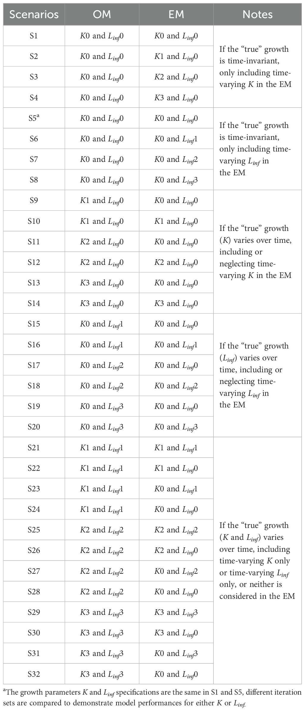
Table 1. Growth parameters K and L_inf specifications in the OM and EM for the 32 model scenarios considered in this study.

2.2 Simulation framework

2.2.1 OM and EM settings

The operating model used in this study was a single-stock, combined sex, one-area model with quarterly time steps for Eastern Atlantic skipjack. Biological and fisheries parameters were configured based on the model settings from the Eastern Atlantic skipjack stock assessment (ICCAT, 2022). To mimic the actual fishery conditions, the operating models included ten fisheries fleets and one survey fleet assumed for harvest. In all operating models, there was no fishing activity during the first 29 years and acted as a burn-in period. A fully selected fishing mortality maintained a constant value of 0.3 to prevent population collapse in subsequent years (ICCAT, 2022).

Catch data and length composition data were generated in different start and end years which varied with fleets (Supplementary Table S1). Sample sizes for length-composition data were 100 in all years. Surveys were designed to occur annually starting in year 90, providing an abundance index with an observation error of 0.12 (ICCAT, 2022).

Fishing selectivity for all fleets was length-based and time-invariant throughout the fishing periods (Supplementary Table S2). Linear growth was assumed from birth to age 1, after which Von Bertalanffy growth was applied, with a maximum age set at age 6. Natural mortality was estimated using Gaertner’s approach (Gaertner, 2015). Fecundity was modeled as a direct function of female body weight, and maturity was modeled with a logistic function. The stock-recruitment relationship followed a Beverton-Holt function. A minor observation error modeled as the standard error of the logarithm of the catch was incorporated in the OM with a default value of 0.005, which was assumed to have a negligible impact on simulation results. Process errors were introduced into the OM by incorporating independent, bias-corrected lognormal deviations to the recruitment.

Estimation models were based on the structure of the operating models, following the actual stock assessment process by estimating model parameters and quantities of management interest. Priors for the input parameters were set to the same values as the priors in the operating models. Detailed information regarding biological parameters and how they were estimated in the EM was provided in Supplementary Table S3.

2.2.2 Link growth to sea surface temperature

Regarding temporal variations in the “true” growth of skipjack driven by the climate-induced sea surface temperature, we introduced the relationships between the growth coefficient K and water temperature (Equation 2), which was outlined by Mallet et al. (1999). The growth parameter K is modeled using the function of Rosso et al. (1995).

$\begin{array}{ll}K(T)=K_{opt}\frac{(T-T_{min}) (T-T_{max})}{(T-T_{min}) (T-T_{max})-{(T-T_{opt})}^2}& (2)\end{array}$

where T represents water temperature, T_min and T_max denote the minimal and maximal growth temperatures, respectively, and K_opt represents the optimal growth parameter at the optimal water temperature, T_opt. The shape of this equation is similar to a parabola, where K is equal to 0 at T_min and T_max, peaking at the optimal values K_opt at T_opt, which has biological significance. For skipjack, the minimal and maximal growth temperatures were determined as 15 °C and 33 °C, respectively, on the basis of the findings of Dizon et al. (1977). The optimal water temperature T_opt was taken to be 26.2 °C, as reported by Boyce et al. (2008). Additionally, K_opt was estimated to be 0.569 from the growth-temperature equation using water temperature data.

In this simulation, time-varying L_inf was considered to have a direct relationship related to the growth parameter K via Pauly’s growth performance parameter μ (Equation 3) (Pauly, 1979). It was suggested that fish of a given genotype either exhibit a low growth coefficient, K, and a high asymptotic length, L_inf, or vice versa, but the value of μ remains constant despite environmental variations (Pauly, 1991). This corresponds to the widely accepted negative correlation between these two parameters (Kimura, 2008).

$\begin{array}{ll}{L}_{inf}(T)=\sqrt{\frac{{10}^{\mu }}{K(T)}}& (3)\end{array}$

Environmental-driven growth variation can be incorporated into stock assessments by modifying the growth function parameters. In SS3, environmental data can be linked to the growth parameters in various forms, such as linear, exponential or logistic (Methot and Wetzel, 2013). Given the assumed relationship between growth and water temperature, as well as the input data requirements, we applied the optimal forms, i.e., an exponential relationship for the temporal variation in both the growth rate K and the asymptotic length L_inf (Equations 3, 4).

$\begin{array}{ll}{K}_t=K_{base} e^{{\beta }_K E_t}& (4)\end{array}$

$\begin{array}{ll}{L}_{inft}=L_{infbase} e^{{\beta }_{L_{inf}} E_t}& (5)\end{array}$

where β_K and ${\beta }_{L_{inf}}$ are the parameters linking the growth parameters to the environmental data, K_base and $L_{infbase}$ are annual mean values for the growth rate and asymptotic length calculated from the relationships between growth and water temperature, and E_t represents the environmental input data. Since the link parameters β_K and ${\beta }_{L_{inf}}$ cannot be estimated directly from the SST data, we used a sea surface temperature index transformed by the Z-score method (Cheadle et al., 2003) as a proxy for SST. The link parameters β_K and ${\beta }_{L_{inf}}$ for the operating models were estimated by the “true” time-varying growth calculated from the temperature-dependent growth model (Supplementary Table S4).

2.3 Sea surface temperature data sources

The SST data associated with growth parameters of the historical climate condition were obtained from the NOAA Extended Reconstructed Sea Surface Temperature (ERSST V5) dataset¹ (Huang et al., 2017). The yearly SST time series were generated by calculating the average SST over the Eastern Atlantic skipjack catch region (latitudes 20°S~40°N and longitudes 35°W~20°E). For the future climate condition, the SST data were extracted from the output of the global climate model CESM2 WACCM, developed by the U.S. National Center for Atmospheric Research (NCAR), under the context of the SSP5-8.5 and the SSP1-2.6². The yearly SST time series were generated by calculating the average monthly SST over the same catch region. The delta change method (Maraun, 2016) was used to standardize the SST data to ensure the comparability of SST time series across different climate conditions. The standardized SST time series for both the historical and future climate conditions are shown in Figure 1.

Figure 1

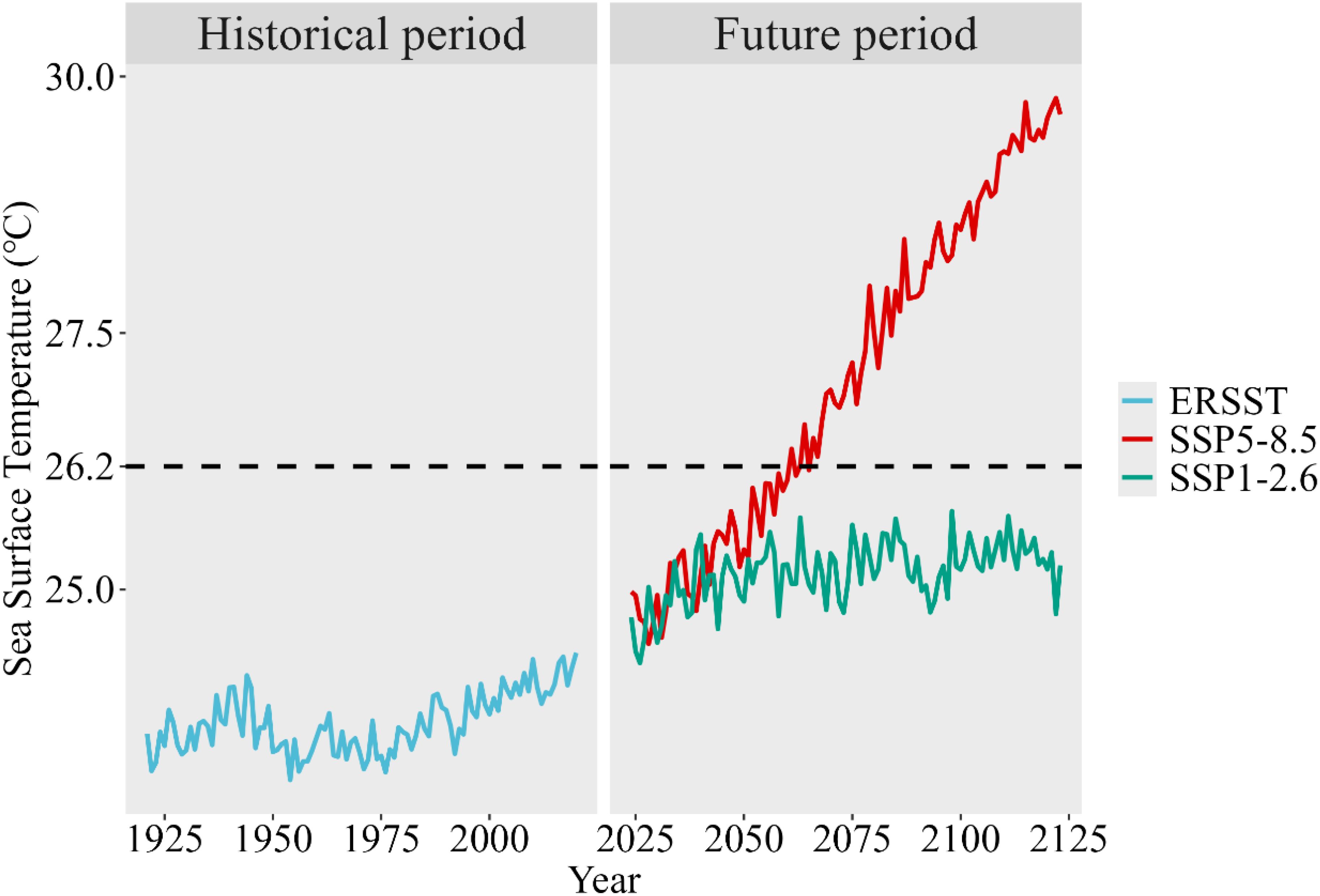
Figure 1. Standardized SST time series using delta change method. The black dashed line represents the optimal water temperature T_opt for skipjack.

2.4 Performance metrics

The model performance across various scenarios was assessed by comparing the relative differences in the quantities of management interest between the operating models and the estimation models. We used relative error (RE) to quantify both bias and precision (Kindong et al., 2023), median relative error (MRE) to quantify bias for all time scales, median absolute relative error (MARE) to quantify precision for all time scales (Dai et al., 2023). The RE, MRE, and MARE were as estimated thus (Equations 6–8).

$\begin{array}{ll}RE=(\widehat{\theta }-\theta )/\theta & (6)\end{array}$

$\begin{array}{ll}MRE=median[(\widehat{\theta }-\theta )/\theta ]& (7)\end{array}$

$\begin{array}{ll}MARE=median[|(\widehat{\theta }-\theta )/\theta |]& (8)\end{array}$

where $\widehat{\theta }$ represents the estimated values of quantities of management interest from the estimation models, $\theta$ corresponds to the “true” values derived from the operating models. The values closer to zero for three performance metrics signify less bias and more precision in the model estimates. The 50% and 90% quantiles for the relative errors are also calculated. The metric could provide insights into the bias of the model estimates associated with various growth parameter assumptions.

3 Results

Most of the iterations successfully converged (Supplementary Table S5), as indicated by a maximum gradient less than 1×10^-4 with no parameters estimated on specified bounds for which a positive definite Hessian matrix could be estimated. The manual tuning commonly applied in a stock assessment is impractical in this simulation study (Monnahan et al., 2016; Stawitz et al., 2019). Therefore, the failed iterations were discarded and excluded from the subsequent results.

3.1 Including temporal growth variation in the assessment when the “true” growth is time-invariant

When the “true” growth parameters were time-invariant, including time-varying K in the EM introduced fluctuations in the relative error of the quantities of management interest, particularly for the historical climate condition and future climate condition of SSP 5-8.5 (Figure 2 S1–S4). In the future climate condition of the SSP1-2.6, the estimated quantities of management interest resembled the bias pattern observed under S1 (Figure 2 S4). The estimated stock depletion in the future climate condition of SSP 5-8.5 showed greater bias and imprecision, with a MARE value 0.063 higher compared to the estimates under S1 (Table 2). The estimated SSB/SSB_MSY in the terminal year showed minimal discrepancy across these scenarios, with MRE values close to zero. While the MRE values for the estimated F/F_MSY in the terminal year also remained close to zero, the error distributions were more dispersed (Figure 3).

Figure 2

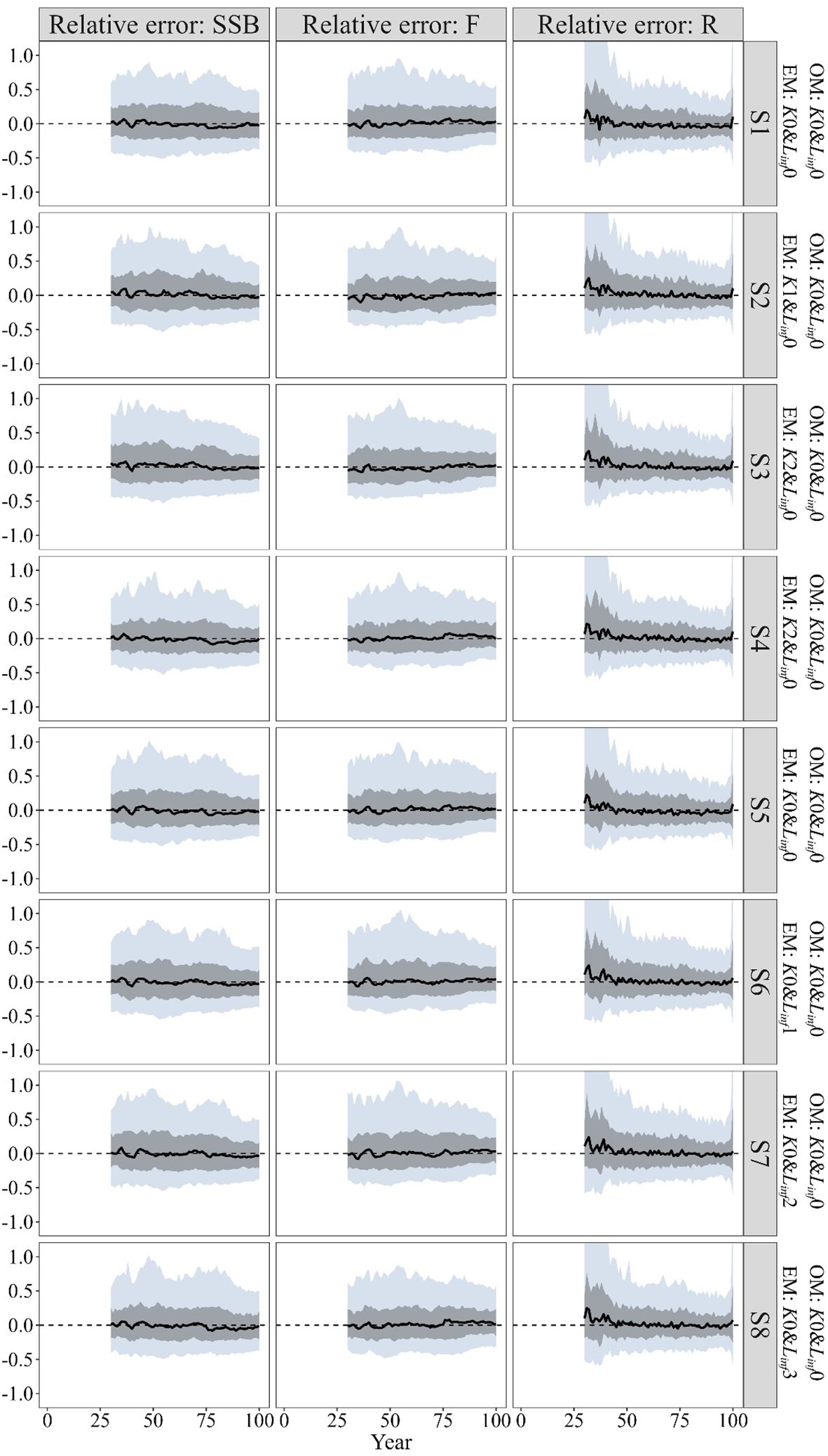
Figure 2. Time trajectories of relative error (RE) for the quantities of management interest (spawning stock biomass SSB, fishing mortality F and recruitment R) for only including time-varying K in the EM (S1~S4) and only including time-varying L_inf in the EM (S5~S8) when “true” growth parameters are time-invariant. The grey and light blue regions cover 50% and 90% of relative errors, and the solid lines represent the median relative errors (MRE). All graphical elements (median lines and confidence regions) in the time trajectories plots below are consistently with this description.

Table 2

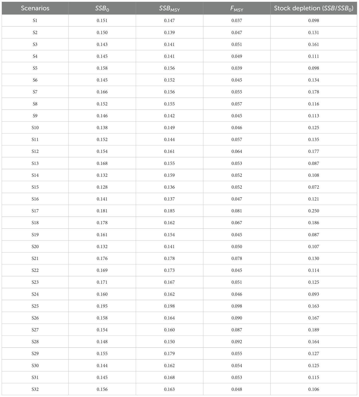
Table 2. Median absolute relative error (MARE) in quantities of management interest across all scenarios.

Figure 3

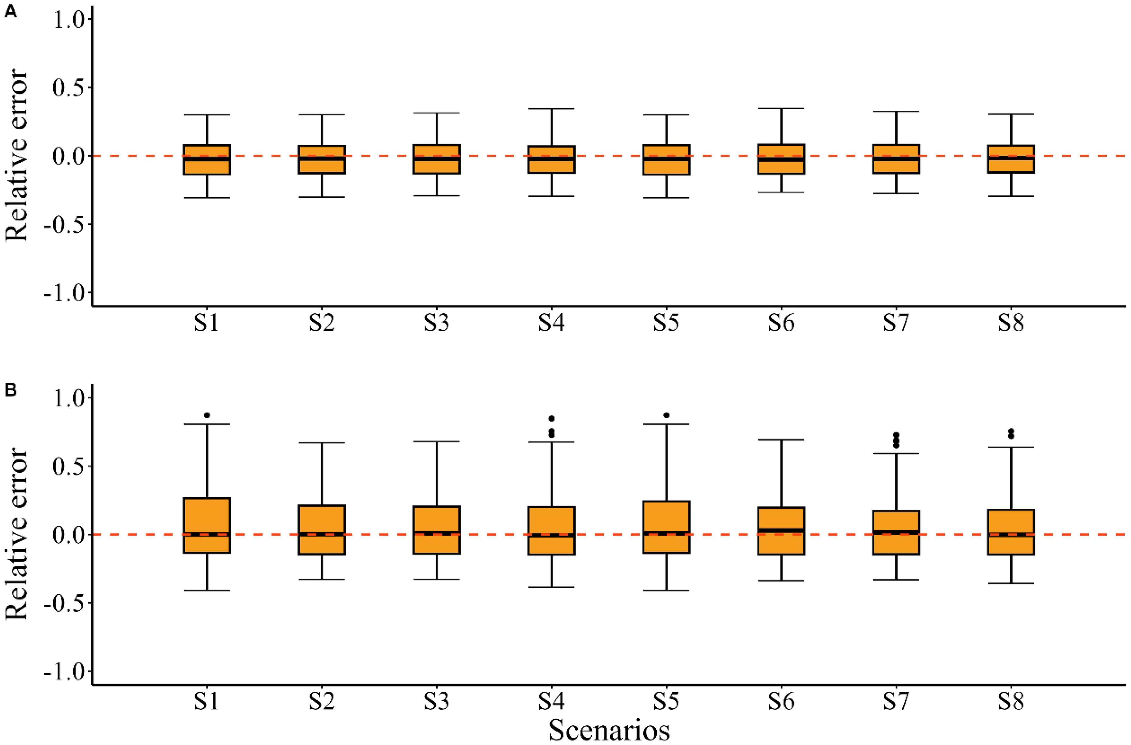
Figure 3. Relative errors (RE) for the estimated SSB/SSB_MSY (A) and F/F_MSY (B) in the terminal year for scenarios S1~S8. The black solid lines in the boxes represent the median relative errors (MRE), the whiskers of the boxplots extend to the maximum and minimum values within 1.5 × IQR (interquartile range), with values beyond this range classified as outliers that visualized as black dots. All graphical elements (median lines, whiskers, and outliers) in the boxplots below are consistently with this description.

When the “true” growth parameters were time-invariant and only time-varying L_inf was included in the EM, the model performance mirrored the bias pattern seen in the K-associated scenarios above, introducing bias in the quantities of management interest (Figure 2 S5–S8). This was particularly evident for the estimated stock depletion in the future climate condition of SSP 5-8.5, which had a MARE value 0.08 higher compared to the estimates under S1 (Table 2). For the estimated SSB/SSB_MSY and F/F_MSY in the terminal year, S5~S8 showed similar error distributions with MRE values close to zero (Figure 3).

3.2 Misspecification of temporal growth variation (when the “true” growth (K or L_inf) varies over time)

When the “true” growth parameter K was time-varying, compared to misspecifying K as time-invariant (i.e. using a constant K), including time-varying K in the EM showed limited capacity to improve the quantities of management interest across different climate conditions (Figure 4 S9–S14; Table 2). For the estimated SSB/SSB_MSY in the terminal year, the MRE values were close to zero in most scenarios, except for S13, where a slight bias was observed (Figure 5). The results for the estimated F/F_MSY in the terminal year further highlighted the limited improvement from including time-varying K, as indicated by the slight bias in S12 compared to the estimates under S11 (Figure 5).

Figure 4

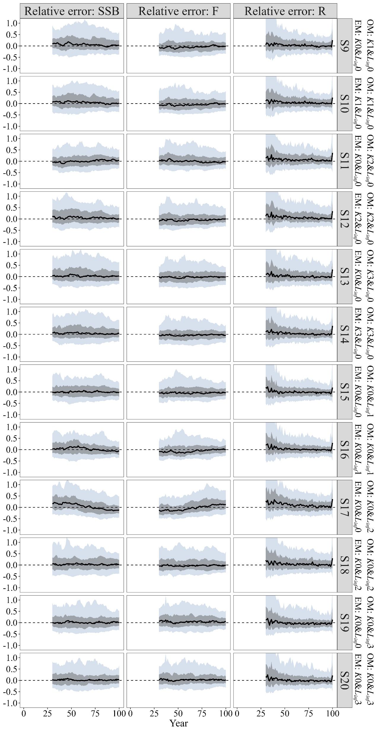
Figure 4. Time trajectories of relative errors (RE) for the quantities of management interest (SSB, F, and R) when only growth parameter K is time-invariant in the OM (S9~S14) and when only growth parameter L_inf is time-invariant in the OM (S15~S20).

Figure 5

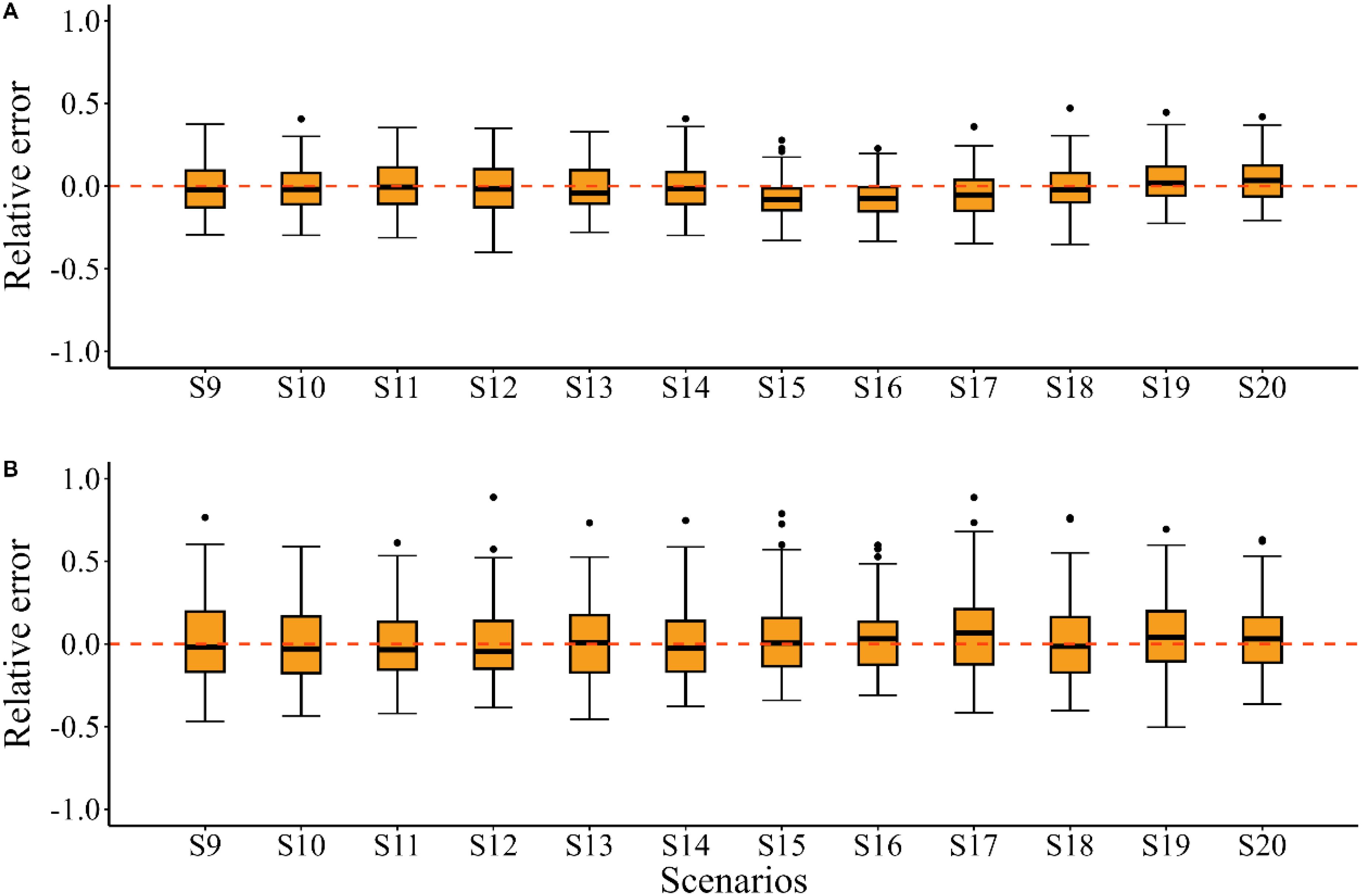
Figure 5. Relative errors (RE) for the estimated SSB/SSB_MSY (A) and F/F_MSY (B) in the terminal year for scenarios S9~S20.

When the “true” growth parameter L_inf was time-varying, model performances varied across different climate conditions. In S15 and S16, including time-varying L_inf in the EM did not improve the quantities of management interest compared to using a constant value, with evident bias in the estimations of SSB and F (Figure 4 S15, S16). For the future climate condition of SSP5-8.5, misspecifying L_inf as time-invariant in the EM introduced significant bias in the quantities of management interest (Figure 4 S17, S18), with the MARE value for estimated stock depletion being 0.064 higher (Table 2). However, for the future climate condition of SSP1-2.6, including time-varying L_inf in the EM resulted in slight improvements, with the median relative error for SSB and F estimates close to zero (Figure 2, S19, S20). The estimated SSB/SSB_MSY and F/F_MSY in the terminal year exhibited similar bias patterns to the other quantities of management interest discussed earlier (Figure 5).

3.3 Misspecification of temporal growth variation (when the “true” growth (K and L_inf) varies over time)

For the historical climate condition, when the “true” growth parameters were time-varying, misspecifying the growth parameters as time-invariant (i.e. including only time-varying K, only time-varying L_inf, or using constant K and L_inf) in the EM resulted in similar bias pattern in the estimated SSB and F as those observed with correctly specified growth parameters (Figure 6 S21–S24). Among these, the inclusion of only time-varying L_inf (S23) resulted in fewer fluctuations in MRE values for the estimated SSB and F compared to the other scenarios. A comparison of MARE values for other quantities of management interest revealed that including more time-varying growth parameters in the EM brought more bias and imprecision (Table 2 S21–S24). The estimated SSB/SSB_MSY in the terminal year demonstrated less bias and smaller error distributions when using constant K and L_inf instead of including both time-varying growth parameters in the EM (Figure 7). Furthermore, no evident bias was observed across these scenarios for the estimated F/F_MSY in the terminal year (Figure 7).

Figure 6

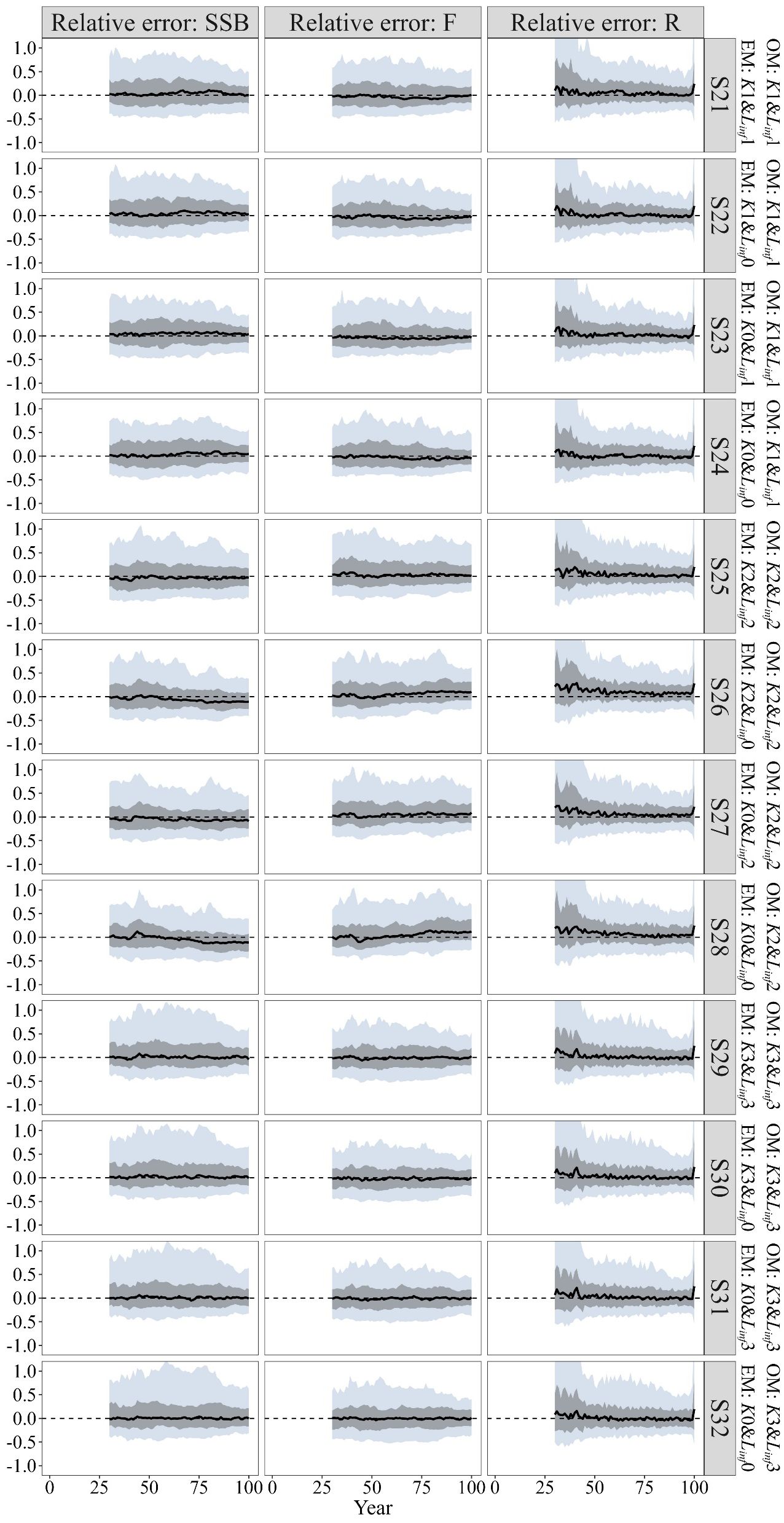
Figure 6. Time trajectories of relative errors (RE) for the quantities of management interest (SSB, F, and R) when “true” growth parameters are time-varying for the historical climate condition (S21~S24), for the future climate condition of SSP5-8.5 (S25~S28) and for the future climate condition of SSP1-2.6 (S29~S32).

Figure 7

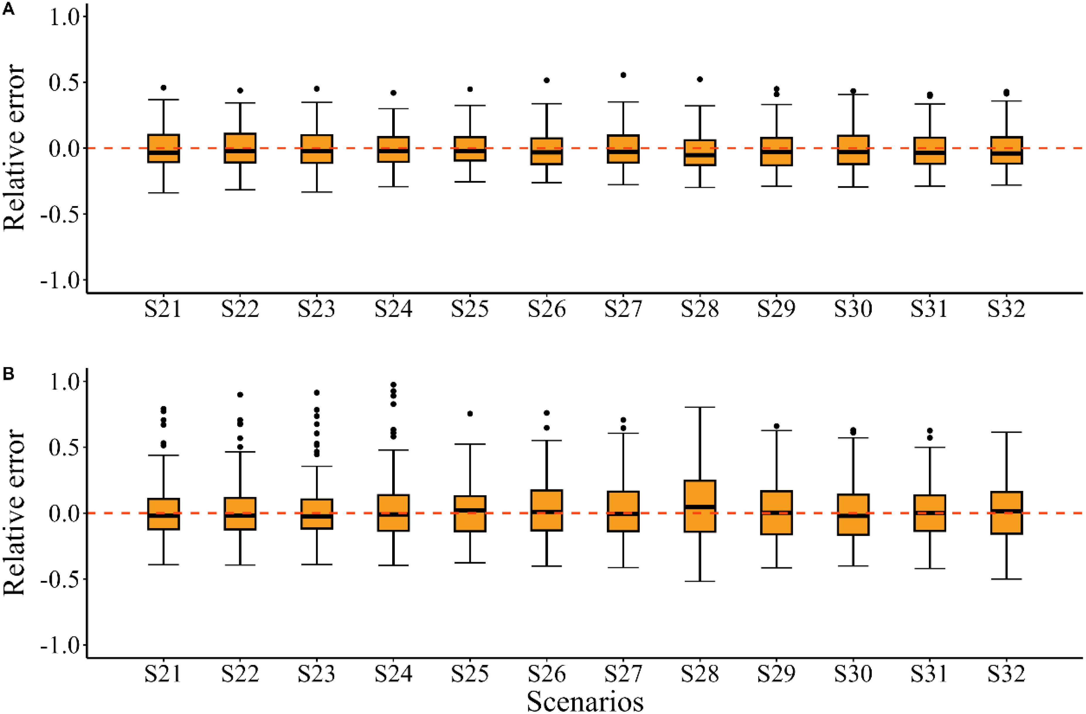
Figure 7. Relative errors (RE) for the estimated SSB/SSB_MSY (A) and F/F_MSY (B) in the terminal year for scenarios S21~S32.

For the future climate condition of SSP5-8.5, the model with correctly specified time-varying growth parameters (S25) outperformed the other scenarios (S26~S28). Evident underestimated bias in SSB and overestimated bias in F were observed when growth parameters were misspecified as time-invariant in the EM (Figure 6 S25–S28). Among these misspecified models, including only time-varying L_infperformed better than including only time-varying K or using constant K and L_inf in the EM, as indicated by fewer fluctuations in MRE values for the quantities of management interest (Figure 6 S26–S28). The correctly specified growth parameters in the EM also outperformed the other scenarios in estimating stock depletion, as evidenced by MARE values that were 0.001 to 0.026 lower (Table 2). Additionally, less bias and smaller error distributions were observed in the estimated SSB/SSB_MSY and F/F_MSY in the terminal year under S25, while S28 showed an underestimated bias in SSB/SSB_MSY in the terminal year and an overestimated bias in F/F_MSY in the terminal year (Figure 7).

For the future climate condition of SSP1-2.6, little discrepancy was observed in the bias patterns of the estimated SSB and F across scenarios with correctly specified and misspecified growth parameters in the EM, with MRE values for these quantities of management interest remaining close to zero (Figure 6 S29–S32). Compared to S29, estimating fewer link parameters in the EM (S30~S32) slightly improved the results for the quantities of management interest (Table 2). For the estimated SSB/SSB_MSY and F/F_MSY in the terminal year, the bias pattern in S31 which included only time-varying L_inf was more similar to that of S29 among these scenarios, exhibiting minimal underestimated bias and smaller error distributions (Figure 7).

4 Discussion

We evaluated model performance for correctly specified and misspecified temporal growth variation across different climate conditions. Misspecification of growth parameters in the estimation models was found to introduce bias in the estimated quantities of management interest in most cases, regardless of whether the “true” growth varied with time. Compared to incorporating time-varying L_inf, the inclusion of time-varying K showed a limited capacity to improve the accuracy and precision of the estimated quantities of management interest when the “true” temporal growth variation existed. Our findings indicated that the estimated quantities of management interest, in particular, the SSB-associated quantities (e.g., stock depletion) were more sensitive to the inclusion of time-varying L_inf than to time-varying K.

Empirical evidence from experimental studies on the ontogenetic growth of various fish species suggests that warming affects the asymptotic length of fish in diverse ways (Barneche et al., 2019; Huss et al., 2019; Lindmark et al., 2022). These studies indicate that asymptotic length is more likely to be influenced by the temperature selecting for different life histories (Lindmark, 2020). For Atlantic skipjack, it has been suggested that individuals inhabiting waters south of 10°N latitude tend to grow larger than those found North of 10°N latitude (Gaertner et al., 2008). The variation in asymptotic length is recognized to become more pronounced under extreme environmental changes (Ben-Hasan et al., 2024). Additionally, key model estimates such as fishing mortality rate and depletion level have been shown to be highly sensitive to assumptions about asymptotic length, as demonstrated in a case study on tropical tuna species (Aires-da-Silva et al., 2015). The bidirectional misestimation for quantities of management interest carry distinct consequences for fisheries management. The underestimated SSB induced by growth misspecification (e.g., S26~S28 in this study) could lead to overly conservative harvest limits, unnecessarily restricting catches and resulting in economic losses. On the other hand, overestimating SSB could allow for unsustainable fishing intensity and pose a risk of stock collapse, as observed in Atlantic bluefin tuna assessments where growth overestimation concealed the decline of fish stock (Fromentin et al., 2014). While fishing intensity can generally be controlled by measures such as catch limits, restrictions on fishing effort, or the establishment of fishing closures, it is typically more difficult to directly control the biomass or spawning stock biomass of target stocks through management measures. Since fishery managers need to assess whether overfished stocks are recovering through the SSB-associated quantities, temporal variation in fish asymptotic length should be considered a priority in stock assessments that incorporate temporal growth variation.

Disregarding environmental information in the stock assessment models has led to biased estimations of stock status, resulting in the inadvertent depletion of fish stocks (Rijnsdorp et al., 2009). It is essential to proceed with caution, however, when integrating time-varying growth correlated with environmental information into stock assessment models. In reality, while multiple parameters may vary over time, incorporating more variables without a clear understanding of how the environment influences population processes and the relationships between parameters could increase model complexity and degrade model performance (e.g., S12 and S16 in this study). The mistaken choices of time-varying growth would limit the model’s capacity to mimic the true variation (Francis, 2016). It is also an infeasible practice to obtain estimates of time-varying growth parameters if fixing some other model parameters as misspecified values (Stawitz et al., 2019). A desirable approach is to include the models with environmental-related time-varying parameters in the form of an uncertainty grid, whose outputs could be an extension of the confidence interval of estimates of management quantities. In practice, it could provide fishery managers with additional information about the predictable consequences (Stawitz et al., 2019). Compared to the redundant calculations, after all, it is unlikely that any fishery industry stakeholder would willingly accept outcomes such as decreased productivity and stock depletion, yet these occurrences may become more frequent due to inadequate fisheries management based on inaccurate evaluations amidst accelerating climate change (Brander, 2009; Rijnsdorp et al., 2009). Given these thoughts, it is suggested that the inclusion of environmental-related temporal growth variation would be important for the stock assessment of the potential effects of future climate change.

Given that sea surface temperature is an intuitive indicator of climate change, in particular the observed accelerated warming of the Atlantic tropical ocean since 1980 (Muhling et al., 2015; Li et al., 2016; Cheng et al., 2020), and that this trend is expected to continue and intensify throughout the 21st century (Arias et al., 2021), this study adopted the growth parameters linked to sea surface temperature to characterize temporal growth variation. This alternative approach was feasible when directional biological data was unavailable. The environmental index can be better simulated using an autoregressive model with bias correction, as practiced by Lee et al. (2018), where parameters estimated from fish skeletal tissues (e.g., otoliths) more explicitly capture the temporal variation in growth. Additionally, the assumed “true” growth temporal variation within the operating models conforms to the general relationship of growth and environmental influences, which is represented by a nearly parabolic shape. However, the growth parameters in SS3 can only be linked to environmental data in ways that do not account for the “optimal” environmental factor values that are specific to fish species (i.e., lacking biological significance). Therefore, it is suggested to incorporate more alternative options for environmental linkages in time-varying parameters, which could enhance the capacity of ss3sim to better simulate “true” population dynamics.

In this study, we detected the growth variation associated with the yearly effect of climate-driven water warming on the environmentally sensitive species skipjack, and it also should be noted that temporal variation in growth across various cohorts may not be fully considered. Temporal variation in fish growth might be attributed to not only climate-induced environmental changes but also other factors, such as intraspecific or interspecific competition (Sinclair et al., 2002). Individuals within cohorts of fish may display diverse growth rates due to conditions in early life stages, genetic differences and density dependence (Correa et al., 2021). The impacts of cohort-specific temporal growth variation on the performances of stock assessment have been verified but received less attention compared to the year-specific cases. Whitten et al. (2013) compared a standard stock assessment model with static growth to the alternative model with cohort-specific variable growth and found that the alternative model better fitted the data and provided significant results of female spawning depletion. While the impacts of cohort-specific temporal growth variation on the performances of stock assessment may be buffered by short periods with inconsistent growth rates across cohorts, not as significant as year-specific cases (Correa et al., 2021), growth variation may be more pronounced under the higher fishing intensity which is attributed to the swifter decrease in the proportion of fast-growing fish in the cohorts (Francis, 2016). Therefore, priority should be given to accounting for cohort-specific temporal growth variation in the stock assessment for those short-lived fast-growing species with high fishing pressure. The next step of resolution could involve the comprehensive inclusion of both external environmental factors and internal factors driving the temporal growth variation, which would require further work to prioritize understanding the biological, ecological and fishery characteristics of fish species.

The International Commission for the Conservation of Atlantic Tunas (ICCAT), the regional fishery management organization (RFMO) responsible for the conservation and management of Atlantic tuna and tuna-like species, has made efforts to address the potential effects of climate change within its management framework for these species. ICCAT has explicitly integrated climate change considerations into management strategy evaluation (MSE) to develop climate-adaptive management procedures, which has become more common practice than traditional assessment-based management for tuna RFMOs in recent times. For example, operating models are tuned to encompass climate change scenarios to ensure the robustness of the management procedures in North Atlantic swordfish MSE where climate change may have effects on its stock distribution, reproduction, and growth (ICCAT, 2023). Management procedures for Atlantic skipjack are being developed as well. MSE is taken as a potent decision-making tool to allow fishery managers to better understand the consequences of the ‘unknown-unknown’ situation (e.g., nature of fish growth variation) in the context of climate change (Walter et al., 2023). Moreover, the ICCAT Plan of Action on climate change has been presented to the ICCAT Commission. Even though more time is required to assess this Plan given its breadth and implications, ICCAT is ahead of the curve compared to other RFMOs in this regard (ICCAT, 2023). All these efforts highlight ICCAT’s commitment to the proactive conservation and management of Atlantic tuna fisheries in the face of climate change.

Our study provided evidence of the risks associated with not accounting for temporal growth variation under different climate conditions. While there remains a tradeoff between methodology consistency and comprehensiveness in recent fisheries stock assessments, explicitly incorporating the environmental data into stock assessment would be a positive step towards implementing climate-adaptive stock assessment and fisheries management.

Data availability statement

Publicly available datasets were analyzed in this study. This data can be found here: https://www1.ncdc.noaa.gov/pub/data/cmb/ersst/v5/ascii/ and https://www.wdc-climate.de/ui/.

Author contributions

JF: Conceptualization, Data curation, Methodology, Visualization, Writing – original draft. FZ: Conceptualization, Methodology, Writing – review & editing. MS: Writing – review & editing. YC: Methodology, Writing – review & editing. JZ: Funding acquisition, Writing – review & editing.

Funding

The author(s) declare financial support was received for the research, authorship, and/or publication of this article. This study was financially supported by the Program on the Survey, Monitoring and Assessment of Global Fishery Resources sponsored by the Ministry of Agriculture and Rural Affairs of China and the China Scholarship Council (202208310191).

Acknowledgments

We are very grateful to two reviewers for their valuable comments that substantially improved an earlier version of this paper.

Conflict of interest

The authors declare that the research was conducted in the absence of any commercial or financial relationships that could be construed as a potential conflict of interest.

Generative AI statement

The author(s) declare that no Generative AI was used in the creation of this manuscript.

Publisher’s note

All claims expressed in this article are solely those of the authors and do not necessarily represent those of their affiliated organizations, or those of the publisher, the editors and the reviewers. Any product that may be evaluated in this article, or claim that may be made by its manufacturer, is not guaranteed or endorsed by the publisher.

Supplementary material

The Supplementary Material for this article can be found online at: https://www.frontiersin.org/articles/10.3389/fmars.2025.1555106/full#supplementary-material

Footnotes

1. ^ https://www1.ncdc.noaa.gov/pub/data/cmb/ersst/v5/ascii/ Date of last access: February 16, 2023.
2. ^ https://www.wdc-climate.de/ui/cmip6?input=CMIP6.ScenarioMIP.NCAR.CESM2-WACCM.ssp585 https://www.wdc-climate.de/ui/cmip6?input=CMIP6.ScenarioMIP.NCAR.CESM2-WACCM.ssp126 Date of last access: May 14, 2024.

References

Aires-da-Silva A. M., Maunder M. N., Schaefer K. M., Fuller D. W. (2015). Improved growth estimates from integrated analysis of direct aging and tag-recapture data: An illustration with bigeye tuna (Thunnus obesus) of the eastern Pacific Ocean with implications for management. Fisheries Res. 163, 119–126. doi: 10.1016/j.fishres.2014.04.001

Crossref Full Text | Google Scholar

Anderson S. C., Monnahan C. C., Johnson K. F., Ono K., Valero J. L. (2014). ss3sim: an R package for fisheries stock assessment simulation with stock synthesis. PloS One 9, e92725. doi: 10.1371/journal.pone.0092725

PubMed Abstract | Crossref Full Text | Google Scholar

Arias P., Bellouin N., Coppola E., Jones R., Krinner G., Marotzke J., et al. (2021). Climate change 2021: The physical science basis. Contribution working group14 I to sixth Assess. Rep. Intergovernmental Panel Climate Change, 319–329.

Google Scholar

Ashida H., Watanabe K., Tanabe T. (2018). Growth variability of juvenile skipjack tuna (Katsuwonus pelamis) in the western and central Pacific Ocean. Environ. Biol. Fishes 101, 429–439. doi: 10.1007/s10641-017-0708-9

Crossref Full Text | Google Scholar

Barneche D. R., Jahn M., Seebacher F. (2019). Warming increases the cost of growth in a model vertebrate. Funct. Ecol. 33, 1256–1266. doi: 10.1111/fec.2019.33.issue-7

Crossref Full Text | Google Scholar

Ben-Hasan A., Vahabnezhad A., Burt J. A., Alrushaid T., Walters C. J. (2024). Fishery implications of smaller asymptotic body size: Insights from fish in an extreme environment. Fisheries Res. 271. doi: 10.1016/j.fishres.2023.106918

Crossref Full Text | Google Scholar

Boltaña S., Sanhueza N., Aguilar A., Gallardo-Escarate C., Arriagada G., Valdes J. A., et al. (2017). Influences of thermal environment on fish growth. Ecol. Evol. 7, 6814–6825. doi: 10.1002/ece3.2017.7.issue-17

Crossref Full Text | Google Scholar

Boyce D. G., Tittensor D. P., Worm B. (2008). Effects of temperature on global patterns of tuna and billfish richness. Mar. Ecol. Prog. Ser. 355, 267–276. doi: 10.3354/meps07237

Crossref Full Text | Google Scholar

Brander K. (2009). Impacts of climate change on marine ecosystems and fisheries. J. Mar. Biol. Assoc. India 51, 1–13. doi: 10.1038/NCLIMATE2119

Crossref Full Text | Google Scholar

Brett J. (1979). “Environmental factors and growth,” in Fish physiology (New York: Elsevier).

Google Scholar

Britten G. L., Dowd M., Kanary L., Worm B. (2017). Extended fisheries recovery timelines in a changing environment. Nat. Commun. 8, 15325. doi: 10.1038/ncomms15325

PubMed Abstract | Crossref Full Text | Google Scholar

Cheadle C., Vawter M. P., Freed W. J., Becker K. G. (2003). Analysis of microarray data using Z score transformation. J. Mol. diagnostics 5, 73–81. doi: 10.1016/S1525-1578(10)60455-2

PubMed Abstract | Crossref Full Text | Google Scholar

Cheng L., Abraham J., Zhu J., Trenberth K. E., Fasullo J., Boyer T., et al. (2020). Record-setting ocean warmth continued in 2019. Adv. Atmospheric Sci. 37, 137–142. doi: 10.1007/s00376-020-9283-7

Crossref Full Text | Google Scholar

Correa G. M., Mcgilliard C. R., Ciannelli L., Fuentes C. (2021). Spatial and temporal variability in somatic growth in fisheries stock assessment models: evaluating the consequences of misspecification. ICES J. Mar. Sci. 78, 1900–1908. doi: 10.1093/icesjms/fsab096

Crossref Full Text | Google Scholar

Correa G. M., Monnahan C. C., Sullivan J. Y., Thorson J. T., Punt A. E. (2023). Modelling time-varying growth in state-space stock assessments. ICES J. Mar. Sci. 80, 2036–2049. doi: 10.1093/icesjms/fsad133

Crossref Full Text | Google Scholar

Dai L., Hodgdon C. T., Xu L., Wang J., Tian S., Chen Y. (2023). Performance evaluation of catch-only methods when catch data are misreported. Fisheries Res. 258. doi: 10.1016/j.fishres.2022.106520

Crossref Full Text | Google Scholar

Dizon A. E., Neill W. H., Magnuson J. J. (1977). Rapid temperature compensation of volitional swimming speeds and lethal temperatures in tropical tunas (Scombridae). Environ. Biol. Fishes 2, 83–92. doi: 10.1007/BF00001418

Crossref Full Text | Google Scholar

Erauskin-Extramiana M., Arrizabalaga H., Hobday A. J., Cabré A., Ibaibarriaga L., Arregui I., et al. (2019). Large-scale distribution of tuna species in a warming ocean. Global Change Biol. 25, 2043–2060. doi: 10.1111/gcb.14630

PubMed Abstract | Crossref Full Text | Google Scholar

Francis R. C. (2016). Growth in age-structured stock assessment models. Fisheries Res. 180, 77–86. doi: 10.1016/j.fishres.2015.02.018

Crossref Full Text | Google Scholar

Fromentin J.-M., Bonhommeau S., Arrizabalaga H., Kell L. T. (2014). The spectre of uncertainty in management of exploited fish stocks: The illustrative case of Atlantic bluefin tuna. Mar. Policy 47, 8–14. doi: 10.1016/j.marpol.2014.01.018

Crossref Full Text | Google Scholar

Gaertner D., De Molina A. D., Ariz J., Pianet R., Hallier J. P. (2008). Variability of the growth parameters of the skipjack tuna (Katsuwonus pelamis) among areas in the eastern Atlantic: analysis from tagging data within a meta-analysis approach. Aquat. Living Resour. 21, 349–356. doi: 10.1051/alr:2008049

Crossref Full Text | Google Scholar

Gaertner D. (2015). Indirect estimates of natural mortality rates for Atlantic skipjack (Katsuwonus pelamis), using life history parameters. Collect Vol. Sci. Pap. ICCAT 71 (1), 189–204.

Google Scholar

Gamperl A. K., Ajiboye O. O., Zanuzzo F. S., Sandrelli R. M., Ellen De Fátima C. P., Beemelmanns A. (2020). The impacts of increasing temperature and moderate hypoxia on the production characteristics, cardiac morphology and haematology of Atlantic Salmon (Salmo salar). Aquaculture 519, 734874. doi: 10.1016/j.aquaculture.2019.734874

Crossref Full Text | Google Scholar

Harley C. D., Randall Hughes A., Hultgren K. M., Miner B. G., Sorte C. J., Thornber C. S., et al. (2006). The impacts of climate change in coastal marine systems. Ecol. Lett. 9, 228–241. doi: 10.1111/j.1461-0248.2005.00871.x

PubMed Abstract | Crossref Full Text | Google Scholar

Heather F., Childs D., Darnaude A. M., Blanchard J. (2018). Using an integral projection model to assess the effect of temperature on the growth of gilthead seabream Sparus aurata. PloS One 13, e0196092. doi: 10.1371/journal.pone.0196092

PubMed Abstract | Crossref Full Text | Google Scholar

Hilborn R. (2012). The evolution of quantitative marine fisheries management 1985–2010. Natural Resource Modeling 25, 122–144. doi: 10.1111/j.1939-7445.2011.00100.x

Crossref Full Text | Google Scholar

Huang M., Ding L., Wang J., Ding C., Tao J. (2021). The impacts of climate change on fish growth: A summary of conducted studies and current knowledge. Ecol. Indic. 121, 106976. doi: 10.1016/j.ecolind.2020.106976

Crossref Full Text | Google Scholar

Huang B., Thorne P. W., Banzon V. F., Boyer T., Chepurin G., Lawrimore J. H., et al. (2017). NOAA extended reconstructed sea surface temperature (ERSST), version 5. NOAA Natl. Centers Environ. Inf. 30, 25. doi: 10.7289/v5t72fnm

Crossref Full Text | Google Scholar

Huss M., Lindmark M., Jacobson P., Van Dorst R. M., Gårdmark A. (2019). Experimental evidence of gradual size-dependent shifts in body size and growth of fish in response to warming. Global Change Biol. 25, 2285–2295. doi: 10.1111/gcb.2019.25.issue-7

PubMed Abstract | Crossref Full Text | Google Scholar

ICCAT (2022). Report of the 2022 Skipjack stock assessment meeting (Madrid, Spain: ICCAT).

Google Scholar

ICCAT (2023). Report of the ICCAT Climate Change Experts Meeting (Madrid, Spain: ICCAT).

Google Scholar

Jobling M. (2002). Environmental factors and rates of development and growth. Handb. fish Biol. fisheries 1, 97–122.

Google Scholar

Johnson K. F., Monnahan C. C., Mcgilliard C. R., Vert-Pre K. A., Anderson S. C., Cunningham C. J., et al. (2015). Time-varying natural mortality in fisheries stock assessment models: identifying a default approach. ICES J. Mar. Sci. 72, 137–150. doi: 10.1093/icesjms/fsu055

Crossref Full Text | Google Scholar

Jonsson B., Jonsson N. (2009). A review of the likely effects of climate change on anadromous Atlantic salmon Salmo salar and brown trout Salmo trutta, with particular reference to water temperature and flow. J. fish Biol. 75, 2381–2447. doi: 10.1111/j.1095-8649.2009.02380.x

PubMed Abstract | Crossref Full Text | Google Scholar

Kimura D. K. (2008). Extending the von Bertalanffy growth model using explanatory variables. Can. J. Fisheries Aquat. Sci. 65, 1879–1891. doi: 10.1139/F08-091

Crossref Full Text | Google Scholar

Kindong R., Wu F., Sarr O., Zhu J. (2023). A simulation-based option to assess data-limited fisheries off West African waters. Sci. Rep. 13, 15290. doi: 10.1038/s41598-023-42521-3

PubMed Abstract | Crossref Full Text | Google Scholar

Kuriyama P. T., Ono K., Hurtado-Ferro F., Hicks A. C., Taylor I. G., Licandeo R. R., et al. (2016). An empirical weight-at-age approach reduces estimation bias compared to modeling parametric growth in integrated, statistical stock assessment models when growth is time varying. Fisheries Res. 180, 119–127. doi: 10.1016/j.fishres.2015.09.007

Crossref Full Text | Google Scholar

Lam V. W., Allison E. H., Bell J. D., Blythe J., Cheung W. W., Frölicher T. L., et al. (2020). Climate change, tropical fisheries and prospects for sustainable development. Nat. Rev. Earth Environ. 1, 440–454. doi: 10.1038/s43017-020-0071-9

Crossref Full Text | Google Scholar

Lee Q., Thorson J. T., Gertseva V. V., Punt A. E. (2018). The benefits and risks of incorporating climate-driven growth variation into stock assessment models, with application to Splitnose Rockfish (Sebastes diploproa). ICES J. Mar. Sci. 75, 245–256. doi: 10.1093/icesjms/fsx147

Crossref Full Text | Google Scholar

Li X., Xie S.-P., Gille S. T., Yoo C. (2016). Atlantic-induced pan-tropical climate change over the past three decades. Nat. Climate Change 6, 275–279. doi: 10.1038/nclimate2840

Crossref Full Text | Google Scholar

Lindmark M. (2020). Temperature-and body size scaling: effects on individuals, populations and food webs. Acta Universitatis Agriculturae Sueciae.

Google Scholar

Lindmark M., Ohlberger J., Gårdmark A. (2022). Optimum growth temperature declines with body size within fish species. Global Change Biol. 28, 2259–2271. doi: 10.1111/gcb.16067

PubMed Abstract | Crossref Full Text | Google Scholar

Lorenzen K. (2016). Toward a new paradigm for growth modeling in fisheries stock assessments: embracing plasticity and its consequences. Fisheries Res. 180, 4–22. doi: 10.1016/j.fishres.2016.01.006

Crossref Full Text | Google Scholar

Mallet J., Charles S., Persat H., Auger P. (1999). Growth modelling in accordance with daily water temperature in European grayling (Thymallus thymallus L.). Can. J. Fisheries Aquat. Sci. 56, 994–1000. doi: 10.1139/f99-031

Crossref Full Text | Google Scholar

Maraun D. (2016). Bias correcting climate change simulations-a critical review. Curr. Climate Change Rep. 2, 211–220. doi: 10.1007/s40641-016-0050-x

Crossref Full Text | Google Scholar

Maunder M. N., Watters G. M. (2003). A general framework for integrating environmental time series into stock assessment models: model description, simulation testing, and example. Fishery Bulletin. 101 (1), 89–100.

Google Scholar

Meinshausen M., Nicholls Z. R. J., Lewis J., Gidden M. J., Vogel E., Freund M., et al. (2020). The shared socio-economic pathway (SSP) greenhouse gas concentrations and their extensions to 2500. Geosci. Model. Dev. 13, 3571–3605. doi: 10.5194/gmd-13-3571-2020

Crossref Full Text | Google Scholar

Merino G., Arrizabalaga H., Arregui I., Santiago J., Murua H., Urtizberea A., et al. (2019). Adaptation of north Atlantic albacore fishery to climate change: Yet another potential benefit of harvest control rules. Front. Mar. Sci. 6, 620. doi: 10.3389/fmars.2019.00620

Crossref Full Text | Google Scholar

Methot J. R.D., Wetzel C. R. (2013). Stock synthesis: a biological and statistical framework for fish stock assessment and fishery management. Fisheries Res. 142, 86–99. doi: 10.1016/j.fishres.2012.10.012

Crossref Full Text | Google Scholar

Monllor-Hurtado A., Pennino M. G., Sanchez-Lizaso J. L. (2017). Shift in tuna catches due to ocean warming. PloS One 12, e0178196. doi: 10.1371/journal.pone.0178196

PubMed Abstract | Crossref Full Text | Google Scholar

Monnahan C. C., Ono K., Anderson S. C., Rudd M. B., Hicks A. C., Hurtado-Ferro F., et al. (2016). The effect of length bin width on growth estimation in integrated age-structured stock assessments. Fisheries Res. 180, 103–112. doi: 10.1016/j.fishres.2015.11.002

Crossref Full Text | Google Scholar

Muhling B. A., Liu Y., Lee S.-K., Lamkin J. T., Roffer M. A., Muller-Karger F., et al. (2015). Potential impact of climate change on the Intra-Americas Sea: Part 2. Implications for Atlantic bluefin tuna and skipjack tuna adult and larval habitats. J. Mar. Syst. 148, 1–13. doi: 10.1016/j.jmarsys.2015.01.010

Crossref Full Text | Google Scholar

Pauly D. (1979). Gill size and temperature as governing factors in fish growth: a generalization of von Bertalanffy's growth formula. Ber. Inst. f. Merresk. Univ. Kiel. 63, 156.

Google Scholar

Pauly D. (1991). Growth performance in fishes: rigorous description of patterns as a basis for understanding causal mechanisms. ICLARM 4 (3), 3–6.

Google Scholar

Punt A. E. (2023). Those who fail to learn from history are condemned to repeat it: a perspective on current stock assessment good practices and the consequences of not following them. Fisheries Res. 261, 106642. doi: 10.1016/j.fishres.2023.106642

Crossref Full Text | Google Scholar

Punt A. E., Trinnie F., Walker T. I., Mcgarvey R., Feenstra J., Linnane A., et al. (2013). The performance of a management procedure for rock lobsters, Jasus edwardsii, off western Victoria, Australia in the face of non-stationary dynamics. Fisheries Res. 137, 116–128. doi: 10.1016/j.fishres.2012.09.017

Crossref Full Text | Google Scholar

Riahi K., Van Vuuren D. P., Kriegler E., Edmonds J., O’neill B. C., Fujimori S., et al. (2017). The Shared Socioeconomic Pathways and their energy, land use, and greenhouse gas emissions implications: An overview. Global Environ. Change 42, 153–168. doi: 10.1016/j.gloenvcha.2016.05.009

Crossref Full Text | Google Scholar

Rijnsdorp A. D., Peck M. A., Engelhard G. H., Möllmann C., Pinnegar J. K. (2009). Resolving the effect of climate change on fish populations. ICES J. Mar. Sci. 66, 1570–1583. doi: 10.1093/icesjms/fsp056

Crossref Full Text | Google Scholar

Rosso L., Lobry J., Bajard S., Flandrois J.-P. (1995). Convenient model to describe the combined effects of temperature and pH on microbial growth. Appl. Environ. Microbiol. 61, 610–616. doi: 10.1128/aem.61.2.610-616.1995

PubMed Abstract | Crossref Full Text | Google Scholar

Rountrey A. N., Coulson P. G., Meeuwig J. J., Meekan M. (2014). Water temperature and fish growth: otoliths predict growth patterns of a marine fish in a changing climate. Global Change Biol. 20, 2450–2458. doi: 10.1111/gcb.2014.20.issue-8

PubMed Abstract | Crossref Full Text | Google Scholar

Sinclair A., Crawford W. (2005). Incorporating an environmental stock–recruitment relationship in the assessment of Pacific cod (Gadus macrocephalus). Fisheries Oceanography 14, 138–150. doi: 10.1111/j.1365-2419.2005.00326.x

Crossref Full Text | Google Scholar

Sinclair A., Swain D., Hanson J. (2002). Disentangling the effects of size-selective mortality, density, and temperature on length-at-age. Can. J. Fisheries Aquat. Sci. 59, 372–382. doi: 10.1139/f02-014

Crossref Full Text | Google Scholar

Stawitz C. C., Haltuch M. A., Johnson K. F. (2019). How does growth misspecification affect management advice derived from an integrated fisheries stock assessment model? Fisheries Res. 213, 12–21. doi: 10.1016/j.fishres.2019.01.004

Crossref Full Text | Google Scholar

Stock B. C., Miller T. J. (2021). The Woods Hole Assessment Model (WHAM): a general state-space assessment framework that incorporates time-and age-varying processes via random effects and links to environmental covariates. Fisheries Res. 240, 105967. doi: 10.1016/j.fishres.2021.105967

Crossref Full Text | Google Scholar

Thorson J. T., Monnahan C. C., Cope J. M. (2015). The potential impact of time-variation in vital rates on fisheries management targets for marine fishes. Fisheries Res. 169, 8–17. doi: 10.1016/j.fishres.2015.04.007

Crossref Full Text | Google Scholar

Thresher R. E., Koslow J., Morison A., Smith D. (2007). Depth-mediated reversal of the effects of climate change on long-term growth rates of exploited marine fish. Proc. Natl. Acad. Sci. 104, 7461–7465. doi: 10.1073/pnas.0610546104

PubMed Abstract | Crossref Full Text | Google Scholar

Von Bertalanffy L. (1938). A quantitative theory of organic growth (inquiries on growth laws. II). Hum. Biol. 10, 181–213.

Google Scholar

Walter J. III, Peterson C., Marshall K., Deroba J., Gaichas S., Williams B., et al. (2023). When to conduct, and when not to conduct, management strategy evaluations. ICES J. Mar. Sci. 80, 719–727. doi: 10.1093/icesjms/fsad031

Crossref Full Text | Google Scholar

Wang H.-Y., Shen S.-F., Chen Y.-S., Kiang Y.-K., Heino M. (2020). Life histories determine divergent population trends for fishes under climate warming. Nat. Commun. 11, 4088. doi: 10.1038/s41467-020-17937-4

PubMed Abstract | Crossref Full Text | Google Scholar

Weatherley A. (1990). Approaches to understanding fish growth. Trans. Am. Fisheries Soc. 119, 662–672. doi: 10.1577/1548-8659(1990)119<0662:ATUFG>2.3.CO;2

Crossref Full Text | Google Scholar

Whitten A. R., Klaer N. L., Tuck G. N., Day R. W. (2013). Accounting for cohort-specific variable growth in fisheries stock assessments: a case study from south-eastern Australia. Fisheries Res. 142, 27–36. doi: 10.1016/j.fishres.2012.06.021

Crossref Full Text | Google Scholar