The comparisons on wave breaking captured by non-hydrostatic model with or without turbulent dissipation

The spilling and plunging breakers in surf zone are simulated by the non-hydrostatic shock-capturing model with or without turbulent dissipation/model. Geometric and dynamic breaking criteria and wave energy flux are investigated to show the differences on breaking onset and energy dissipation. Comparisons between the k-ϵ and laminar data indicate that both of them give reasonable results, but the absence of turbulent dissipation would cause the seaward movement of breaking point, the underestimation of maximum breaking wave height, and the overprediction of breaking energy loss. And the laminar data presents greater change for velocities near the surface and bottom, resulting in a significantly larger proportion of kinetic energy flux after wave breaking, while the k-ϵ data can give better consistency with the measured in velocity calculations.

1 Introduction

Surface water waves at the transition to breaking are the critical design conditions for marine and coastal structures (Silvester, 1974). Since time immemorial, wave breaking is a great challenge for numerical simulation, due to its rapid changes in wave surface and wave energy, with strong nonlinearity. The numerical methods for wave breaking can be divided into two categories: 1) the combination of wave breaking criteria and energy dissipation mechanics, 2) shock-capturing method. In the shock-capturing method, wave breaking is automatically captured as the weak/discontinuous solution of the governing equations, and the wave-breaking energy is dissipated by numerical dissipation. The shock-capturing methods have been widely used in some famous numerical models, such as OpenFOAM (Jacobsen et al., 2012), SWASH (Zijlema et al., 2011) and NHWave (Ma et al., 2012). SWASH and NHWave are also called non-hydrostatic models, which don’t take hydrostatic pressure assumption in vertical direction, tracking the free surface as a single-valued function. And these shock-capturing models have been compared and validated against many physical experimental results (Castro-Orgaz et al., 2022; Fang et al., 2022; Gao et al., 2021; Gong et al., 2024; Pablo et al., 2013; Qu et al., 2022; Stelling and Zijlema, 2003; Weijie et al., 2022). However, some issues still deserve discussion. For example, the role of turbulent model, the necessity and impact of turbulent dissipation for capturing wave breaking onset and energy loss.

Traditionally, the effect of non-hydrostatic pressure can be included by a Boussinesq-type approximation through adding higher order derivative terms to the nonlinear shallow water equations (NSWE) (Fang et al., 2015; Gao et al., 2023), where a criterion is used to switch from Boussinesq to NSWE (Gao et al., 2024). And wave breaking energy dissipation can be computed by adding dissipation models to the Boussinesq equations (Zijlema and Stelling, 2008), such as eddy viscosity models (Kennedy et al., 2000; Zelt, 1991), roller models (Madsen et al., 1997) and vorticity models based on a transport equation for the breaker-generated vorticity (Roeber et al., 2010; Veeramony and Svendsen, 2000). These models take a trigger or a criterion to provide the onset and termination of wave breaking and a calibration of some tunable parameters inherent in these models is required. Currently, the non-hydrostatic models are based on incompressible Navier-Stokes equations, incorporating the shock-capturing capabilities of Godunov-type schemes to describe wave breaking and other nearshore processes (Zijlema and Stelling, 2008). By considering the similarity between breaking waves and hydraulic jumps, energy dissipation due to turbulence generated by wave breaking is inherently accounted for, but some differences in handling the turbulent dissipation should not be passed over lightly. Viscosity and turbulent dissipation terms are ignored in some non-hydrostatic models, such as SWASH. Using two vertical layers, SWASH gave reasonable computed results for regular wave breaking on a slope, except for the underestimation of wave height at breaking point (Zijlema et al., 2011). He et al. (2020) proposed a non-hydrostatic model based on Euler equations for the numerical investigation of deep-water wave evolution including wave breaking, of which the shock-capturing scheme is different from NHWave. While NHWave applied HLL (Harten-Lax-van Leer) Riemann solver and piecewise linear reconstruction as the shock-capturing scheme for wave breaking, with the Smagorinsky subgrid model for turbulent kinematic viscosity. Derakhti et al. (2016) incorporated the k-ϵ turbulent model into NHWave for wave breaking in the surf zone and deep-water, reporting that $v_t=0$ results in the overprediction of the total wave-breaking-induced energy loss and wave height decay compared with observations. Qu et al. (2024) also used NHWave (volume-averaged k-ϵ turbulence model) to simulate the propagation process of random waves over permeable coral fringing reefs, arguing that the model accurately simulates the wave breaking on the permeable fringing reef. Besides, OpenFOAM uses volume-of-fluid method to track free surface, but also contains dynamic pressure, shock-capturing methods and turbulent dissipation, has also been validated in the simulation of wave breaking (Amini and Memari, 2024; Croquer et al., 2023; Mi et al., 2025; Song et al., 2025; Tsai et al., 2024). Chrysanti et al. (2023) compared laminar and turbulent closure models for dam-break flows using OpenFOAM, reporting that turbulent models achieve better results, but the improvement compared to laminar models is marginal.

According to the research mentioned above, it seems that the shock-capturing non-hydrostatic model could simulate wave breaking accurately regardless of turbulent models. Although it’s well known that wave breaking dissipates through entrainment of air bubbles into the flow and the generation of currents and turbulence. Various turbulent models (such as k-ϵ, k-ω and Renormalized Group) just solve spatial-temporal varying $v_t$ for the Reynolds stress term added in the momentum equations, which works as physical dissipation, in contrast to the numerical dissipation of shock-capturing schemes. Consequently, it’s necessary to investigate the impact on wave breaking in the non-hydrostatic shock-capturing model with or without turbulent dissipation, i.e. physical dissipation and numerical dissipation.

This paper is organized as follows: Section 2 gives a brief description of the present shock-capturing non-hydrostatic model, as well as the details of numerical setup for the cases. Numerical results, comparisons and discussions are given in Section 3, categorized into breaking onset (Section 3.1) and energy dissipation (Section 3.2). Conclusions are presented in Section 4.

2 Numerical model and simulation set-up

The non-hydrostatic shock-capturing used for numerical simulation was developed by He et al. (2020), based on Reynolds-averaged Navier-Stokes (RANS) using the single-value free surface method. This model is the modified version of NHWave, but the third-order weight essential non-oscillation (WENO) scheme and multi-stage (MUSTA) solver are applied instead of the piecewise linear reconstruction and HLL Riemann solver. In other words, the numerical model used here is still a non-hydrostatic shock-capturing model just like NHWave, but with a different shock-capturing scheme. This model has been validated against physical experimental data, including wave breaking in surf zone (He et al., 2022) and deep water (He et al., 2020). Besides, k-ϵ turbulent model is used here to compute the turbulent motion. That is $v_t=C_{\mu }{k}^2/ϵ$, where $v_t$ is the kinematic viscosity, k is the turbulent kinetic energy, ϵ is the turbulent dissipation rate, and $C_{\mu }=0.09$, more details can be referred to He et al. (2022).

Both spilling (hereafter referred as TK1) and plunging (hereafter referred as TK2) cases of Ting and Kirby (1994) are selected to study the impact of turbulent dissipation on wave breaking in surf zone. Figure 1 sketches the layout of computational domain and Table 1 lists the input parameters of incident waves. Regular waves are generated by internal wavemaker, 5 m from the left edge of the numerical tank. This experiment has been widely used by other researchers to validate both non-hydrostatic models using a terrain-following grid, so the parameters and convergence of grid has been discussed much (Derakhti et al., 2016). Generally, the non-hydrostatic model can predict wave propagation well and achieve excellent nonlinearity with a relatively few (three to five) vertical layers (Ma et al., 2012; Panagiotis et al., 2024). In this paper, for both TK1 and TK2, a uniform grid of Δx = 0.025 m is used in x direction (smaller than 1/150 of the wavelength), and 8 uniformly spaced σ-levels in z direction. For each case, the simulations are carried separately for two conditions: with turbulent model (k-ϵ data) and without turbulent model (laminar data).

Figure 1

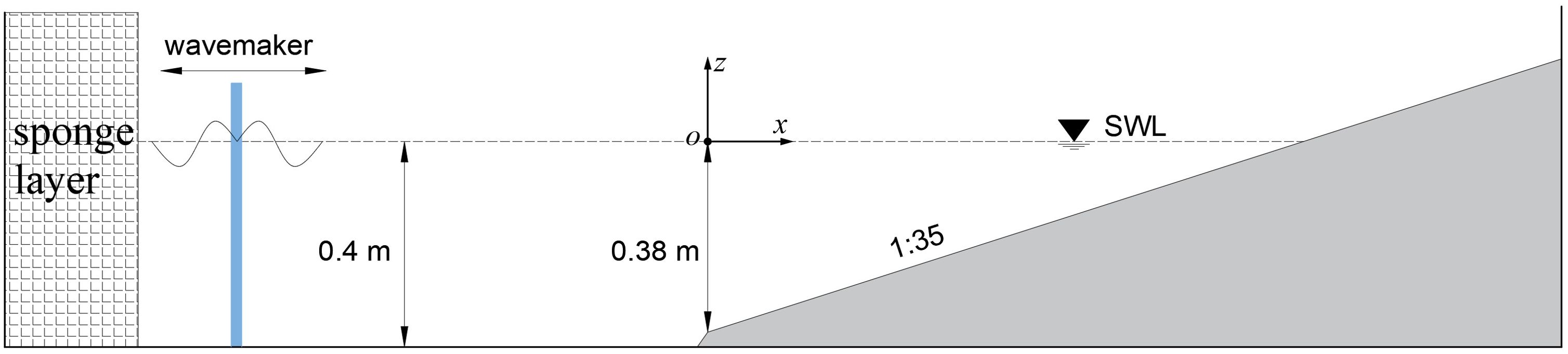
Figure 1. The layout of computational domain for TK1 and TK2.

Table 1

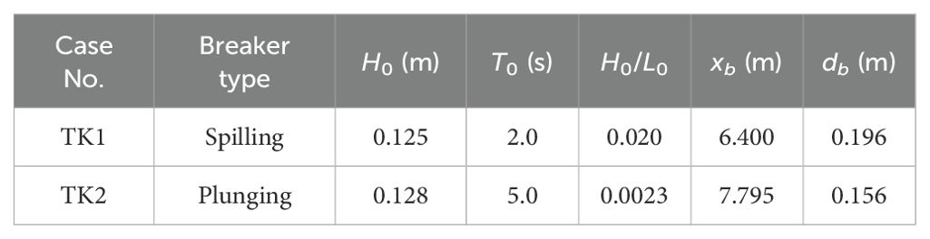
Table 1. Incident wave conditions (H₀, T₀ and L₀ are respectively the wave height, period and wave length of incident wave; x_b and d_b are the horizontal location and depth of the breaking point).

For TK1 and TK2, the wave heights in horizontal region are very close, i.e., about 0.13 m. But the wave period is increased from 2 s to 5 s, resulting in the ratio of wave height to wavelength of the plunging breaker TK2 is 0.0023, about one tenth of the spilling breaker TK1. As described in physical experiments, though the turbulent bores from the spilling breaker are similar visually to those from the plunging breaker, their flow fields are different, as well as the breaking strength and turbulence intensities. Here, TK1 and TK2 are chosen for simulation and comparison, investigating the discrepancies in wave breaking process with or without turbulent models.

3 Results and discussions

The breaking onset and the energy dissipation are non-trivial problems in the numerical simulation of wave breaking, involving changes in wavefront, velocity fields and wave energy. Therefore, the following discussions are organized by 3.1 breaking onset and 3.2 breaking energy dissipation, to study the effect of turbulent model.

3.1 Breaking onset

Firstly, the distribution of the mean wave height $\overline{H}$ and mean surface elevation $\overline{\eta }$ are presented to give an overview of the differences in simulated results. As shown in Figure 2, The distribution of wave height for the spilling breaker TK1 and plunging breaker TK2 is validated against measured data. In terms of wave height, the increase due to shoaling and the sharp decrease after wave breaking are presented for all results. It seems that both k-ϵ and laminar results are reasonable except some relatively small differences, showing agreement with the measured data generally. Perhaps it can be inferred that with or without turbulent models would not have the distortion of results for wave breaking simulation in the present non-hydrostatic model. What’s more, the differences between k-ϵ and laminar results are varied before and after wave breaking. Next, the differences will be discussed further, including the geometry and dynamic characteristics for breaking onset.

Figure 2

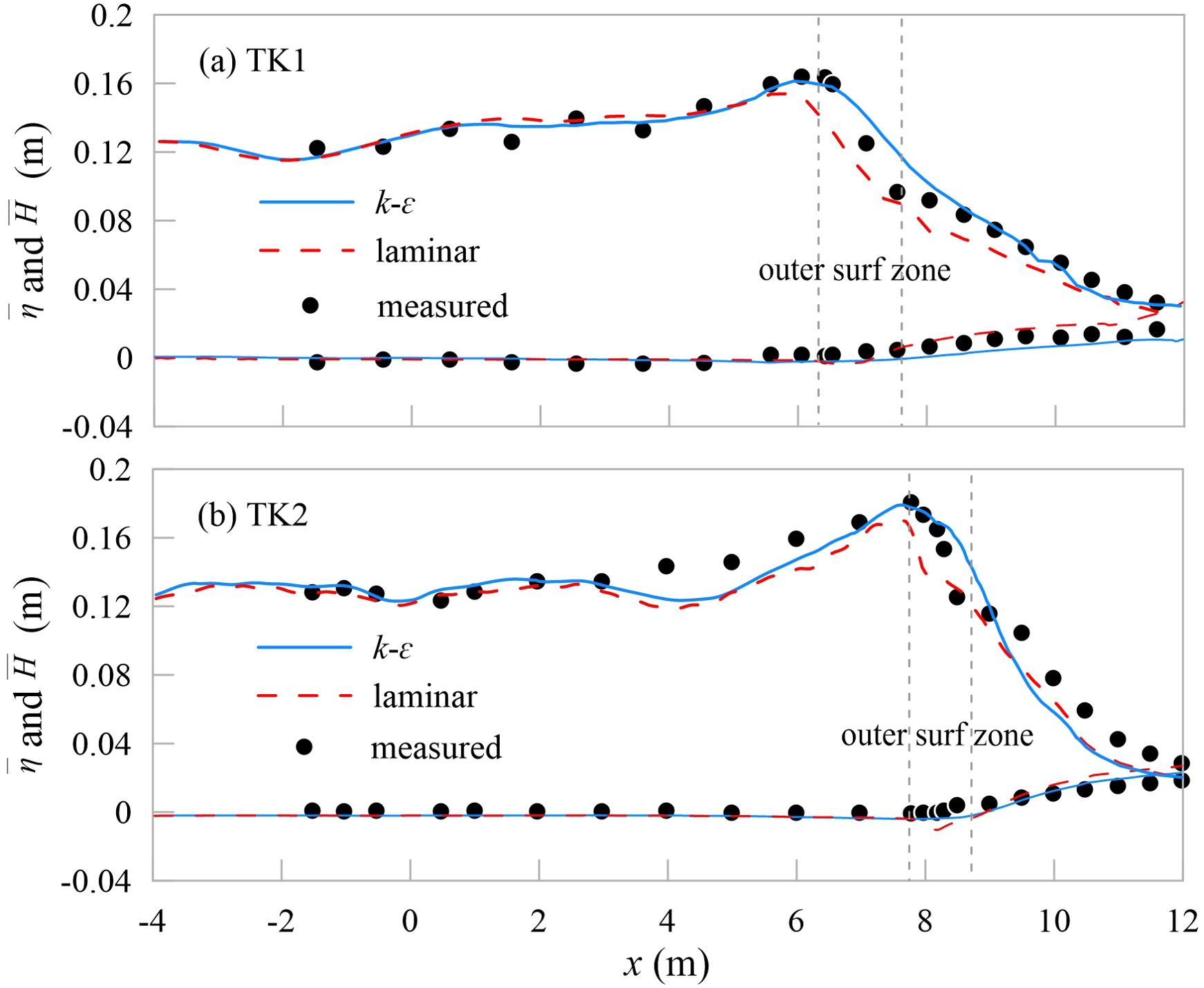
Figure 2. Distribution of mean wave height and mean surface elevation for (A) TK1 and (B) TK2.

Clearly, in both TK1 and TK2, the curves of $\overline{H}$ and $\overline{\eta }$ for the k-ϵ and laminar results are almost identical in upstream of the breaking point, especially in the horizontal region (x< 0 m). Because the turbulence intensities are weak before wave breaking, and laminar flow dominates the wave motion. However, with wave shoaling, the difference increases near the breaking points. Actually, the maximum of wave height in the laminar data is smaller than the k-ϵ data, as listed in Table 2, about 0.07 m. Besides, the breaking points for the k-ϵ and laminar results are not the same, listed in Table 2. In all cases, the computed breaking points are in the upstream of the measured breaking points. That is partially due to the varied definitions of breaking points. In physical experiments, breaking points of spilling breakers are defined as the location where air bubbles begin to be entrained in the wave crest (x_b = 6.40 m), whereas those of plunging breakers are defined as the point where the front face of the wave becomes nearly vertical (x_b = 7.795 m). But in this non-hydrostatic shock-capturing model, the wave breaking onset is captured as the weak solution with the shock-capturing scheme. And the wave front rolling and bubble blending cannot be simulated by this model with the single-value free surface technique. So, in the simulated results, x_b is defined as the point where the maximum wave height is observed. In both TK1 and TK2, the breaking points of the laminar data are ahead of the k-ϵ data (about 0.2 m difference), indicating that wave breaks earlier without turbulent model. In terms of the breaking points and the maximum wave heights, turbulent dissipation has an impact, but relatively small. Therefore, other wave geometry parameters are introduced to give further study next. For example, the ratio of wave height to water depth at the breaking point H_b/d_b is a measurable quantity which can be used to predict the breaking onset and distinguish the types of breakers, of which the value was reported 0.73 – 1.03 (Galvin, 1972). The measured data gives the limiting ratio 0.82 for TK1 and 1.2 for TK2. Because of the deviation of wave height and breaking points, the ratios of the laminar results are smaller than the turbulent results, but the k-ϵ results are closer to the measured data, namely 0.79 and 1.11.

Table 2

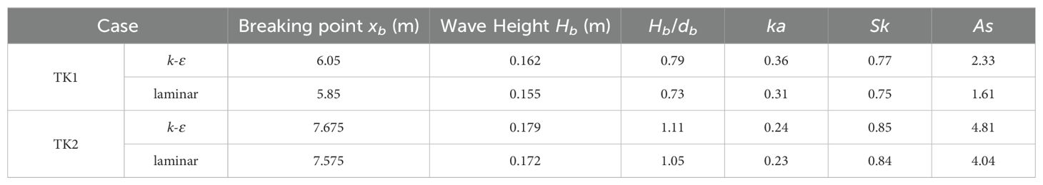
Table 2. Local wave geometry characteristics for simulated results.

Besides, the limiting wave steepness ka associated with incipient wave breaking has been examined extensively. It might be attributed to the varied turbulence intensities. In fact, the limiting steepness ranges from 0.15 to 0.41 in previous studies (Perlin et al., 2013), related to the different methods of breaking-wave generation and ambiguity in the definition of incipient breaking waves. In this paper, k=π/(L₁+L₂) is the local wavenumber calculated based on two consecutive zero-crossing adjacent to the breaking crest, a = (2H_c+H_r+H_f)/4 is the local crest amplitude related to the breaking crest and two adjacent troughs (Derakhti and Kirby, 2016; Kjeldsen and Myrhaug, 1979), as shown in Figure 3. Other geometry parameters are also introduced here to quantify breaking-wave geometry (see Figure 3), namely Asymmetry (As) and Skewness (Sk). For both TK1 and TK2, the ka of k-ϵ data is greater, but not significant differences. It’s noted that the steepness ka of TK1 is greater than that of TK2, because the incident wave heights are similar but the periods are more than double. And other authors also noticed that steepness of some spillers was considerably higher than that of some plungers, which indicated that the magnitude of wave steepness does not always correlate well with wave-breaking strength. As for As and Sk, both of TK1 and TK2, the k-ϵ results give slightly higher values compared to the laminar results. That means turbulent models have greater vertical and horizontal asymmetry for breaking crest, the nonlinearity in k-ϵ data is relatively greater than that in laminar data. All the geometry characteristics mentioned above were investigated to predict the wave breaking onset, but many authors reported varied critical values. It is noteworthy that predicting breaking onset from only geometric aspects might fail, considering the wave profile close to breaking has an irregular shape and complicated definitions. Some authors (Drazen et al., 2008) identified possible connections between the breaking onset and the breaking-wave dynamics, and proposed dynamic breaking criteria based on energy dissipation and dissipation rate. Next, a unified breaking onset threshold parameter B (Barthelemy et al., 2018) for surface gravity waves in arbitrary depth is applied to give further study on the impact of breaking onset caused by turbulent dissipation.

Figure 3

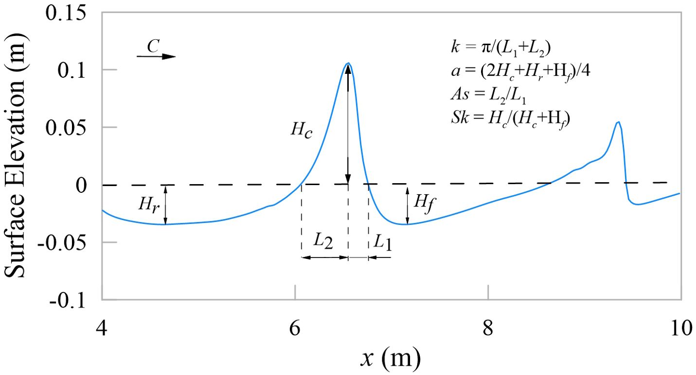
Figure 3. Definitions of local wave geometry.

In 2D situation (x-direction), the breaking parameter B is based on the local wave energy flux F normalized by the local wave energy density E and the wave crest speed c, defined at the maximum elevation of the crest. B can be written as the following dimensionless quantities:

$\begin{array}{ll}B=F/(Ec)& \text{(1.1)}\end{array}$

where,

$\begin{array}{ll}F=u\left(p+\rho g(z-z_0)+\frac{1}{2}\rho \left(u^2+v^2+w^2\right)\right)& \text{(1.2)}\end{array}$

and,

$\begin{array}{ll}E=\rho g(z-z_0)+\frac{1}{2}\rho \left(u^2+v^2+w^2\right)& \text{(1.3)}\end{array}$

Where p is the pressure, u, v, w are the velocity components in x, y, z directions respectively. And z is the vertical coordinate, z₀ is the datum chosen as twice the depth of the flow domain. The breaking threshold for parameter B is B_th =0.85 ± 0.02, which has validity and robustness in varying bathymetry. So, B can be considered as a dynamical criterion to study breaking onset of TK1 and TK2 from the perspective of wave energy.

Figures 4, 5 show snapshots of free surface elevations before and after breaking crest (t* = 0 here, the maximum peak), as well as the temporal variation of B for the evolving wave crest for TK1 and TK2, respectively. In all cases, the parameter B always exceed the breaking inception threshold value B_th =0.85 ± 0.02 (represented with horizontal yellow bar) and keep increasing after breaking onset. Comparing the k-ϵ data and the laminar data, the curves of parameter B are very similar, but some small oscillations are observed in the curves of k-ϵ data. In the laminar data of TK2, oscillations also appear behind the sharp wave fronts, which is consistent with the phenomenon reported by Derakhti et al. (2016). Comparing the spilling breaker TK1 with the plunging breaker TK2, results also show that as the strength of breaking increases, the rate of change in B near the breaking threshold increases.

Figure 4

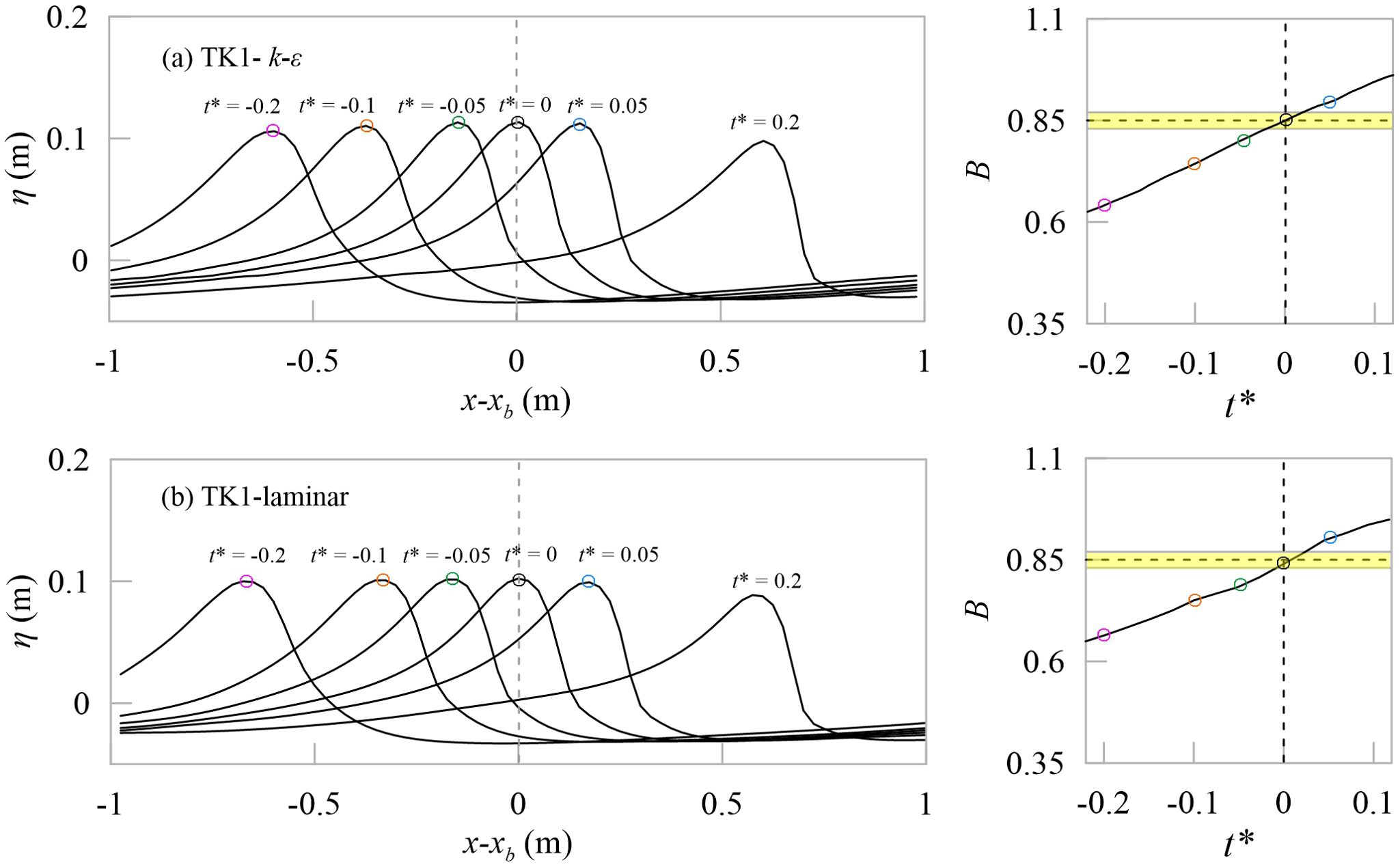
Figure 4. Snapshots of free surface elevations and temporal evolution of the breaking onset parameter B for (A) the k-ϵ and (B) the laminar data of TK1. Here, normalized t* = (t – t_b)/T₀.

Figure 5

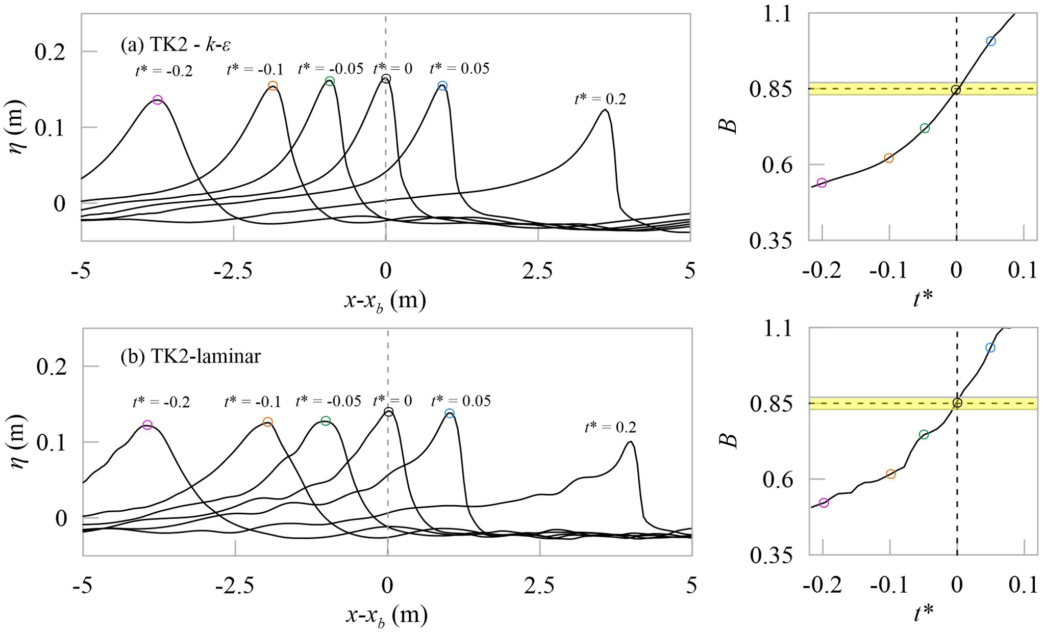
Figure 5. Snapshots of free elevations and temporal evolution of the breaking onset parameter B for (A) the k-ϵ and (B) the laminar data of TK2. Here, normalized t* = (t – t_b)/T₀ represents time offset with respect to breaking time.

According to the discussion above, it’s believed that breaking onsets are captured correctly in all cases, whether geometric criteria or dynamic criteria. So, in shock-capturing non-hydrostatic model, wave breaking onset can be captured without turbulent models, and turbulent dissipation plays little direct role in incipient breaking. That is probably due to the turbulence intensities are weak before wave breaking. Besides, some small differences of maximum wave heights and breaking points should not be passed over lightly. The outer surf zone for the measured data is remarked with two vertical dash lines (see Figure 2), between the breaking point x_b and x_outer, where waves break most strongly. Here x_outer is defined as the point where ${(H_{rms}/H_{rms0})}^2=0.75$ (Ruju et al., 2012), H_rms0 being the offshore root mean square wave height. The difference between the k-ϵ data and the laminar data is most significant in the outer surf zone. The mean wave heights are underpredicted in the outer surf zone, and the k-ϵ data shows greater consistency with the measured data. Given the positive correlation between wave energy and wave height, it’s very necessary to discuss the impact on energy dissipation bought by k-ϵ model, and the increasement of turbulence intensities after breaking onset.

3.2 Energy dissipation

The time-averaged depth-integrated horizontal energy flux of 2D waves per unit width over the time t₁ – t₂, i.e. $\overline{F}$, is defined as the sum of kinetic energy flux ${\overline{F}}_k$ and potential energy flux ${\overline{F}}_p$, can be written as:

$\begin{array}{ll}\overline{F}(x)={\overline{F}}_k(x)+{\overline{F}}_p(x)& \text{(1.4)}\end{array}$

Where

$\begin{array}{ll}{\overline{F}}_k(x)=\frac{1}{t_2-t_1}{\displaystyle {\int }_{t_1}^{t_2}{\displaystyle {\int }_{-h}^{\eta }u[1/2(u^2+w^2)]}}\rho dzdt& \text{(1.5)}\end{array}$

$\begin{array}{ll}{\overline{F}}_p(x)=\frac{1}{t_2-t_1}{\displaystyle {\int }_{t_1}^{t_2}{\displaystyle {\int }_{-h}^{\eta }u[p+\rho gz]}}dzdt& \text{(1.6)}\end{array}$

The Equations 1.5, 1.6 are exact solutions and the spatial variations of the normalized horizontal flux $\overline{F}/{\overline{F}}_0$ for TK1 and TK2 are shown in Figure 6, ${\overline{F}}_0$ being the energy flux at deep water. We can observe the approximate horizontal segment near x – x_b = -8 m (the toe of slope), meaning little energy dissipation here. As the waves propagate towards the shore, the wave energy flux decreases before the breaking point (x – x_b< 0). But with linear, shallow-water approximation, the mean energy flux reads $\overline{F}\propto H^2\sqrt{gh}$. So that decrease of the energy flux upstream of the breaking point is mainly due to shallower water depth, instead of wave breaking. And the outer surf zone for the k-ϵ data is represented by two vertical grey dash lines, where the rapid reduction of energy flux appears, with strong wave breaking. In both TK1 and TK2, the curves of laminar data are just slightly lower than the k-ϵ data, indicating the energy loss is overpredicted without turbulent dissipation. And the similarity proves that the shock-capturing scheme of the present non-hydrostatic model works well in wave breaking energy loss with or without the turbulent model. Besides, $\overline{F}/{\overline{F}}_0$ decreases by 30% in the outer surf zone for both TK1 and TK2, but the outer surf zone of TK1 is about 1.8 m, wider than that of TK2 (about 1.4 m).

Figure 6

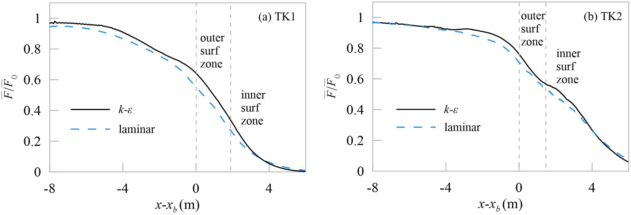
Figure 6. Spatial variations of the normalized horizontal energy flux $\overline{F}/{\overline{F}}_0$ for (A) TK1 and (B) TK2. The solid black lines and dashed blue lines indicate the turbulent and the laminar data respectively.

Refer to Stive (1984), the measured mean energy dissipation rate per unit area is given by $-\Delta \overline{F}/\Delta x$, normalized by the incident wavelength L₀ and the energy flux at horizontal area $F_0$. As the average fitting curves shown in Figure 7, the energy dissipation rates are similar between the k-ϵ and the laminar data for the spilling breaker TK1, and the maximum dissipation rate occurs within one wavelength downstream of the breaking point, 0< (x-x_b)/L₀< 1. But for the plunging breaker TK2, two troughs are observed after wave breaking, might be due to the stronger break strength.

Figure 7

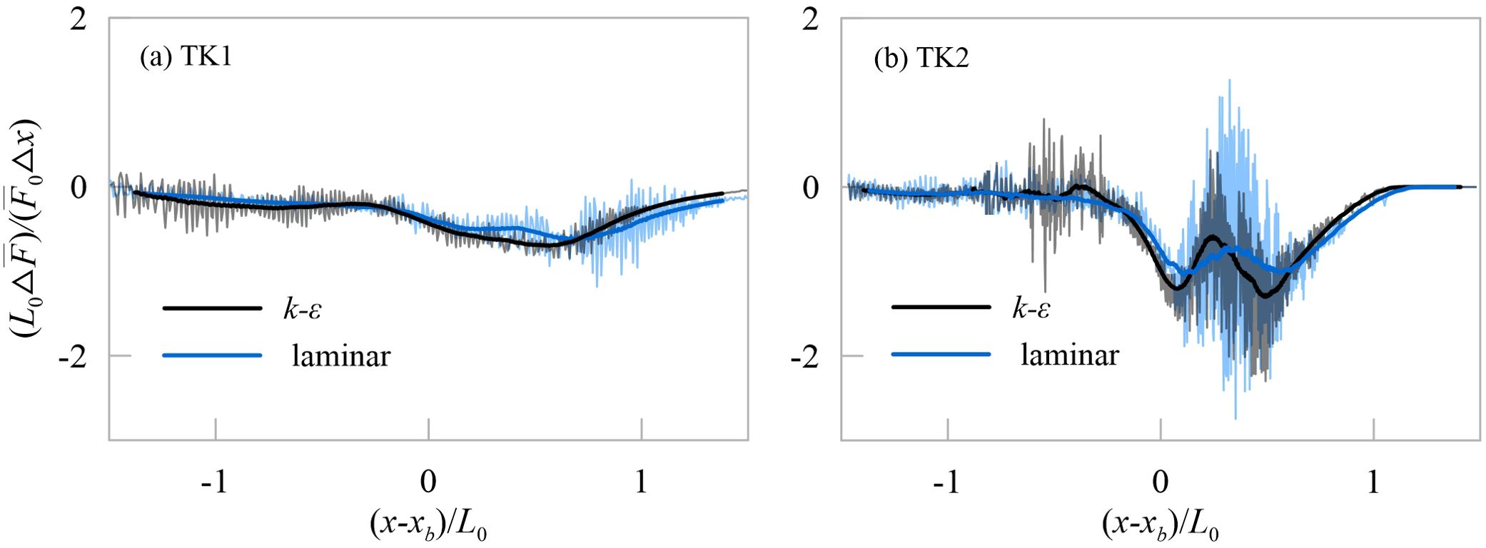
Figure 7. The energy dissipation rate of energy flux $\Delta \overline{F}/\Delta x$ for (A) TK1 and (B) TK2, normalized by the incident wavelength L₀ and the energy flux at horizontal area $F_0$. Thin solid lines are direct calculation of $(L_0\Delta \overline{F})/({\overline{F}}_0\Delta x)$, and heavy solid lines indicate the average fit. The black lines and blue lines indicate the turbulent and the laminar data respectively.

The fractional losses of energy flux are shown in Figure 8, for all cases, the contribution of the kinetic energy flux ${\overline{F}}_E/\overline{F}$ to the total energy flux is much smaller than that of the potential energy flux ${\overline{F}}_p/\overline{F}$ far upstream of the breaking point. But increases up to more than 20% close to the break point, accompanied by the reduction of potential energy flux. Similar changes were reported in constant deep water breaking waves. The growth of ${\overline{F}}_E/\overline{F}$ is kept or even accelerated in the outer surf zone, and reaches its peak close to the right edge, followed by the decrease in the inner surf zone. The changing trends are consistent in the k-ϵ and the laminar data, little difference appears before the breaking point, but the proportion of kinetic energy flux of the laminar is significant larger downstream of the outer surf zone, more than 40%. That means for the laminar computational results, more potential energy flux is transferred to kinetic energy flux in wave breaking. That difference might be attributed to the turbulent motion caused by wave breaking. Figure 9 shows the snapshots of the predicted instantaneous turbulent kinetic energy distribution for TK1 during one period. At t* = 0, the turbulent kinetic energy is relatively small, indicating the turbulence intensity is not the peak at wave breaking onset. At t* = 0.25, 0.5, turbulent motion is strengthening, and the distribution of turbulent kinetic energy is concentrated at the breaking crest front. As the breaking crest propagates towards the shore, the turbulent kinetic energy diffuses to the crest rear, i.e. x-x_b = 0 -2 m. The same trend is also observed in TK2 (not shown here). It’s clear that the turbulent motion originates from instabilities of the surface waves, appears and reduces in sync with wave breaking within one wave cycle. Besides, the turbulence intensities are weak outside the breaking zone. So, due to the absence of turbulent dissipation, the proportion of kinetic energy flux is greater for the laminar data in both TK1 and TK2. And that also indicates that the velocities also might be greater without the turbulent dissipation in the laminar results. To investigate this, Figures 10, 11 present the variations of time-averaged normalized horizontal velocity with depth at several locations for TK1 and TK2.

Figure 8

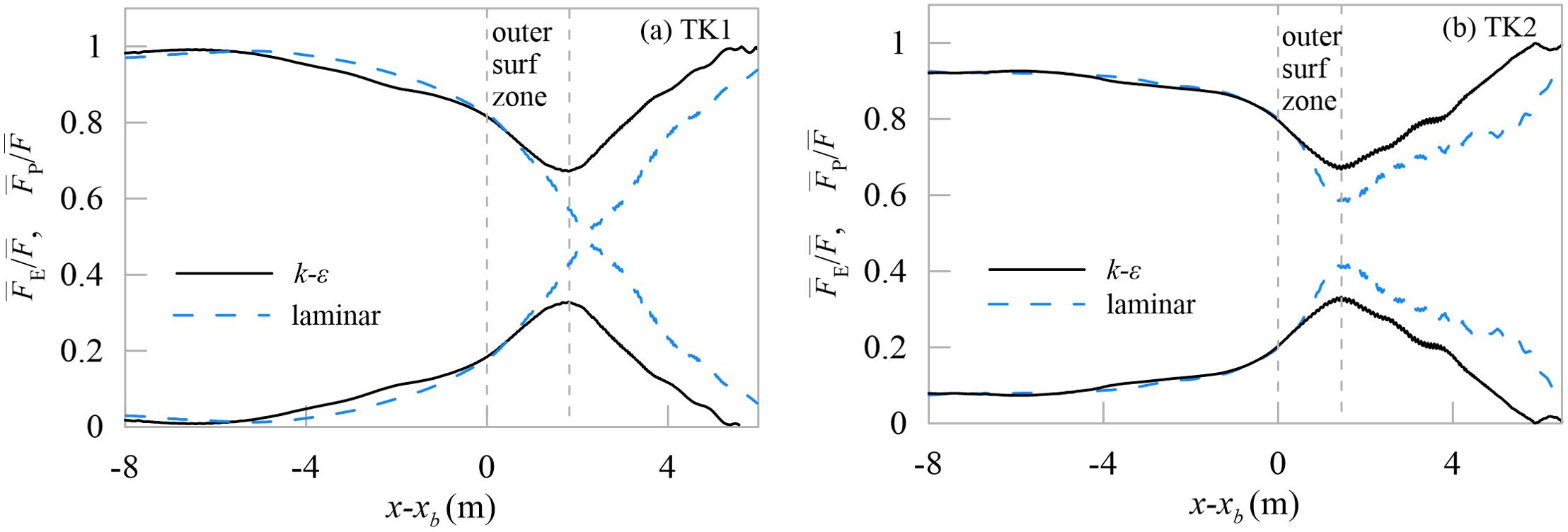
Figure 8. Spatial variations of the ratio of the potential energy flux to the total energy flux ${\overline{F}}_p/\overline{F}$ and the ratio of kinetic energy flux to the total energy flux ${\overline{F}}_k/\overline{F}$ for (A) TK1 and (B) TK2. The solid black lines and dashed blue lines indicate the turbulent and the laminar data respectively.

Figure 9

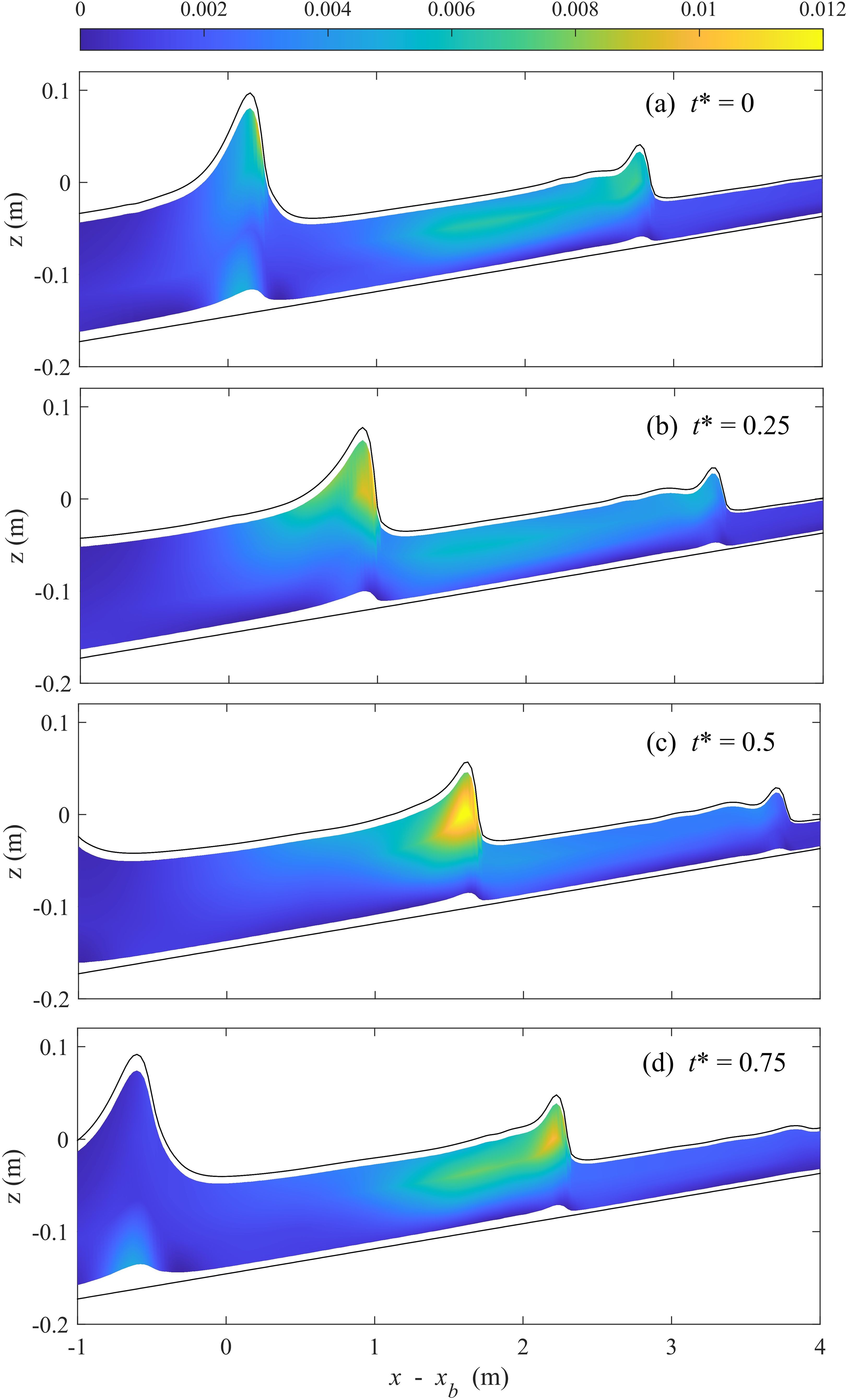
Figure 9. Snapshots of the distribution of turbulent kinetic energy k (m²/s²) for TK1. Here, (A–D) t* = (t -t_b)/T₀ = 0, 0.25,0.5, 0.75 respectively.

Figure 10

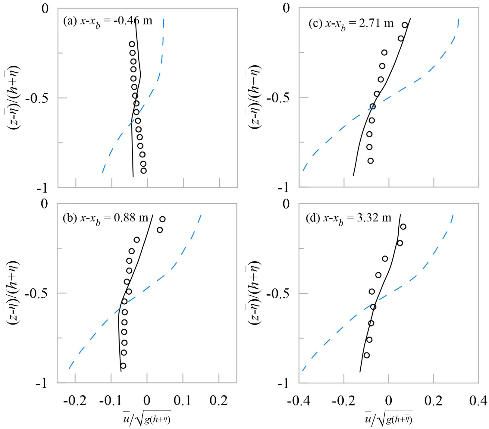
Figure 10. Time-averaged normalized horizontal velocity profiles for TK1 at varied cross-shore locations (A–D) x-x_b = -0.46 m, 0.88 m, 2.71 m, 3.32 m. Circles represent the measured data, black solid lines represent the k-ϵ data, blue dashed lines represent the laminar data.

Figure 11

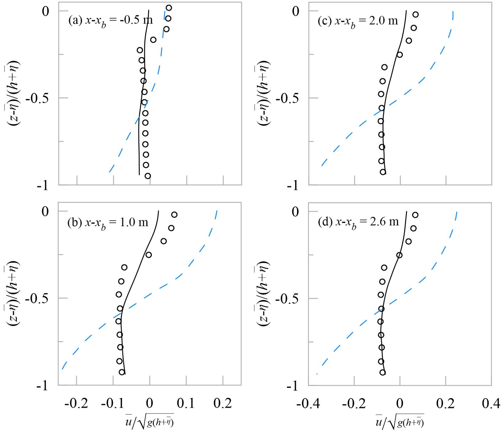
Figure 11. Time-averaged normalized horizontal velocity profiles for TK2 at varied cross-shore locations (A–D) x-x_b = -0.5 m, 1.0 m, 2.0 m, 2.6 m. Circles represent the measured data, black solid lines represent the k-ϵ data, blue dashed lines represent the laminar data.

The time-averaged velocity profiles show the landward current near surface, while seaward current near bottom in all cases, which is consistent with the experimental data. Comparing the k-ϵ and the laminar results, it’s arguable that the k-ϵ results give better agreement with the measured data, while the magnitude of current in the laminar data is significant larger. This difference indicates the velocities and kinetic energy of breaking waves would be overestimated without turbulent dissipation. What’s more, there are significant gradient changes for the measured velocity profiles near the surface, but the k-ϵ data does not capture that sharp turn accurately, might due to the ignorance of the bubble entrainment and the overturning wave front in non-hydrostatic model.

4 Conclusions

In this paper, we investigate wave-breaking simulations in the surf zone using a shock-capturing non-hydrostatic model, which is the revised version of NHWave but with a different shock-capturing scheme (the combination of MUSTA and WENO). For both the spilling breaker TK1 and the plunging breaker TK2, the simulations are carried separately for two conditions: with and without the k-ϵ model. By comparing and analyzing the computed results, the impact on wave breaking bought by turbulent dissipation can be categorized as follows:

(a) Breaking onset: The present model captures the wave breaking onset for both TK1 and TK2, whether it turns on k-ϵ model or not. The calculation and discussion of local wave geometry characteristics (such as the wave steepness ka) and the dynamic breaking onset criteria B prove that the turbulent dissipation causes minor impact on wave breaking in the shock-capturing non-hydrostatic model. As described in all cases, the k-ϵ data and the laminar data show similarities in wave shoaling at slope, the change of wave height before and after wave breaking. But the seaward movement of breaking point and the smaller breaking wave height are also observed in the laminar results, of which the deviations are small.

(b) Energy dissipation: Compared with the k-ϵ results and the measured, the smaller mean wave heights and time-mean energy flux at breaking points and surf zones are observed in the laminar results, indicating more total wave energy loss, but the changes along slope are similar. Furthermore, the proportion of the kinetic energy flux after wave breaking onset is significantly larger without the k-ϵ turbulent model, meaning that more potential energy flux is transferred to kinetic energy flux in wave breaking. Because the velocities are overpredicted without the turbulent dissipation, while the k-ϵ results give better agreement with the measured data.

Therefore, the present shock-capturing non-hydrostatic model can give reasonable results for the wave breaking-onset and total energy loss without turbulent dissipation, but turbulent model is necessary for velocity calculation and presents better consistency with physical experimental data.

Data availability statement

The original contributions presented in the study are included in the article/supplementary material. Further inquiries can be directed to the corresponding author.

Author contributions

DH: Data curation, Investigation, Methodology, Writing – original draft, Writing – review & editing. YH: Data curation, Supervision, Writing – review & editing. HM: Conceptualization, Supervision, Writing – review & editing. JL: Formal Analysis, Validation, Writing – review & editing.

Funding

The author(s) declare that financial support was received for the research, authorship, and/or publication of this article. This work was supported by the Fund of Guangdong Provincial Key Laboratory of Intelligent Equipment for South China Sea Marine Ranching (2023B1212030003); Zhanjiang Non-funded Science and Technology Project (No. 2024B01064), the Program for Scientific Research Start-up Funds of Guangdong Ocean University (No. 060302072303), the National Natural Science Foundation of China (No. 52001071), the Guangdong Basic and Applied Basic Research Foundation (No. 2023A1515010890, No. 2022A1515240039), the Guangdong Basic and Applied Basic Research Foundation (No. 2024A1515012321); and the Open Fund of State Key Laboratory of Coastal and Offshore Engineering, Dalian University of Technology (No. LP2403).

Conflict of interest

The authors declare that the research was conducted in the absence of any commercial or financial relationships that could be construed as a potential conflict of interest.

Generative AI statement

The author(s) declare that no Generative AI was used in the creation of this manuscript.

Publisher’s note

All claims expressed in this article are solely those of the authors and do not necessarily represent those of their affiliated organizations, or those of the publisher, the editors and the reviewers. Any product that may be evaluated in this article, or claim that may be made by its manufacturer, is not guaranteed or endorsed by the publisher.

References

Amini M., Memari A. M. (2024). CFD evaluation of regular and irregular breaking waves on elevated coastal buildings. Int. J. Civil Eng. 22, 333–358. doi: 10.1007/s40999-023-00898-2

Crossref Full Text | Google Scholar

Barthelemy X., Banner M. L., Peirson W. L., Fedele F., Allis M., Dias F. (2018). On a unified breaking onset threshold for gravity waves in deep and intermediate depth water. J. Fluid Mechanics 841, 463–488. doi: 10.1017/jfm.2018.93

Crossref Full Text | Google Scholar

Castro-Orgaz O., Cantero-Chinchilla F. N., Chanson H. (2022). Shallow fluid flow over an obstacle: higher-order non-hydrostatic modeling and breaking waves. Environ. Fluid Mechanics 22, 971–1003. doi: 10.1007/s10652-022-09875-0

Crossref Full Text | Google Scholar

Chrysanti A., Song Y., Son S. (2023). Comparative study of laminar and turbulent models for three-dimensional simulation of dam-break flow interacting with multiarray block obstacles. J. Korea Water Resour. Assoc. 56, 1059–1069. doi: 10.3741/JKWRA.2023.56.S-1.1059

Crossref Full Text | Google Scholar

Croquer S., Díaz-Carrasco P., Tamimi V., Poncet S., Lacey J., Nistor I. (2023). Modelling wave–structure interactions including air compressibility: A case study of breaking wave impacts on a vertical wall along the Saint-Lawrence Bay. Ocean Eng. 273, 113971. doi: 10.1016/j.oceaneng.2023.113971

Crossref Full Text | Google Scholar

Derakhti M., Kirby J. T. (2016). Breaking-onset, energy and momentum flux in unsteady focused wave packets. J. Fluid Mechanics 790, 553–581. doi: 10.1017/jfm.2016.17

Crossref Full Text | Google Scholar

Derakhti M., Kirby J. T., Shi F., Ma G. (2016). Wave breaking in the surf zone and deep-water in a non-hydrostatic RANS model. Part 1: Organized wave motions. Ocean Model. 107, 125–138. doi: 10.1016/j.ocemod.2016.09.001

Crossref Full Text | Google Scholar

Drazen D. A., Melville W. K., Lenain L. (2008). Inertial scaling of dissipation in unsteady breaking waves. J. Fluid Mechanics 611, 307–332. doi: 10.1017/S0022112008002826

Crossref Full Text | Google Scholar

Fang K., Liu Z., Zou Z. (2015). Fully nonlinear modeling wave transformation over fringing reefs using shock-capturing Boussinesq model. J. Coast. Res. 32, 164–171. doi: 10.2112/JCOASTRES-D-15-00004.1

Crossref Full Text | Google Scholar

Fang K., Xiao L., Liu Z., Sun J., Dong P., Wu H. (2022). Experiment and RANS modeling of solitary wave impact on a vertical wall mounted on a reef flat. Ocean Eng. 244, 1–15. doi: 10.1016/j.oceaneng.2021.110384

Crossref Full Text | Google Scholar

Galvin C. J. (1972). “Wave breaking in shallow water,” in Waves on Beaches & Resulting Sediment Transport, editor. Meyer, R. E. Proceedings of an advanced seminar, conducted by the mathematics research center, the University of Wisconsin, and the Coastal Engineering Research Center, U. S. Army, at Madison. 413–456.

Google Scholar

Gao J., Hou L., Liu Y., Shi H. (2024). Influences of bragg reflection on harbor resonance triggered by irregular wave groups. Ocean Eng. 305, 1–22. doi: 10.1016/j.oceaneng.2024.117941

Crossref Full Text | Google Scholar

Gao J., Ma X., Dong G., Chen H., Zang J. (2021). Investigation on the effects of Bragg reflection on harbor oscillations. Coast. Eng. 9, 103977. doi: 10.1016/j.coastaleng.2021.103977

Crossref Full Text | Google Scholar

Gao J., Shi H., Zang J., Liu Y. (2023). Mechanism analysis on the mitigation of harbor resonance by periodic undulating topography. Ocean Eng. 281, 1–16. doi: 10.1016/j.oceaneng.2023.114923

Crossref Full Text | Google Scholar

Gong S., Gao J., Song Z., Shi H., Liu Y. (2024). Hydrodynamics of fluid resonance in a narrow gap between two boxes with different breadths. Ocean Eng. 311, 1–12. doi: 10.1016/j.oceaneng.2024.118986

Crossref Full Text | Google Scholar

He D., Ma Y., Dong G., Perlin M. (2020). Predicting deep water wave breaking with a non-hydrostatic shock-capturing model. Ocean Eng. 216, 108041. doi: 10.1016/j.oceaneng.2020.108041

Crossref Full Text | Google Scholar

He D., Ma Y., Dong G., Perlin M. (2022). A numerical investigation of wave and current fields along bathymetry with porous media. Ocean Eng. 244, 1–14. doi: 10.1016/j.oceaneng.2021.110333

Crossref Full Text | Google Scholar

Jacobsen N. G., Fuhrman D. R., Freds?E J. R. (2012). A wave generation toolbox for the open-source CFD library: OpenFoam. Int. J. Numerical Methods Fluids 70, 0–0. doi: 10.1002/fld.v70.9

Crossref Full Text | Google Scholar

Kennedy A. B., Chen Q., Kirby J. T., Dalrymple R. A. (2000). Boussinesq modeling of wave transformation, breaking, and runup. I:1D. J. Waterway Port Coast. Ocean Eng. 126 (1), 39–47. doi: 10.1061/(ASCE)0733-950X(2000)126:1(39)

Crossref Full Text | Google Scholar

Kirby T. J. T. (1994). Observation of undertow and turbulence in a laboratory surf zone. Coast. Engineering. 24 (1–2), 51–80. doi: 10.1016/0378-3839(94)90026-4

Crossref Full Text | Google Scholar

Kjeldsen S. P., Myrhaug D. (1979). “Breaking waves in deep water and resulting wave forces,” in Proceedings of the Annual Offshore Technology Conference, Houston, Texas. doi: 10.4043/3646-MS

Crossref Full Text | Google Scholar

Ma G., Shi F., Kirby J. T. (2012). Shock-capturing non-hydrostatic model for fully dispersive surface wave processes. Ocean Model. 43-44, 22–35. doi: 10.1016/j.ocemod.2011.12.002

Crossref Full Text | Google Scholar

Madsen P. A., Srensen O. R., Schffer H. A. (1997). Surf zone dynamics simulated by a Boussinesq type model. Part I. Model description and cross-shore motion of regular waves. Coast. Eng. 32, 255–287. doi: 10.1016/S0378-3839(97)00028-8

Crossref Full Text | Google Scholar

Mi C., Gao J., Song Z., Liu Y. (2025). Hydrodynamic wave forces on two side-by-side barges subjected to nonlinear focused wave groups. Ocean Eng. 317, 120056. doi: 10.1016/j.oceaneng.2024.120056

Crossref Full Text | Google Scholar

Pablo H., Javier L. L., Inigo J. L. (2013). Simulating coastal engineering processes with OpenFOAM^®. Coast. Eng. 71, 119–134. doi: 10.1016/j.coastaleng.2012.06.002

Crossref Full Text | Google Scholar

Panagiotis V., Georgios K., Marcel Z., Vasiliki S., Peter T. (2024). A study of the non-linear properties and wave generation of the multi-layer non-hydrostatic wave model SWASH. Ocean Eng. 302, 117633. doi: 10.1016/j.oceaneng.2024.117633

Crossref Full Text | Google Scholar

Perlin M., Choi W., Tian Z. (2013). Breaking waves in deep and intermediate waters. Annu. Rev. Fluid Mechanics 45, 115–145. doi: 10.1146/annurev-fluid-011212-140721

Crossref Full Text | Google Scholar

Qu K., Liu T. W., Chen L., Yao Y., Kraatz S., Huang J. X., et al. (2022). Study on transformation and runup processes of tsunami-like wave over permeable fringing reef using a nonhydrostatic numerical wave model. Ocean Eng. 243, 110228. doi: 10.1016/j.oceaneng.2021.110228

Crossref Full Text | Google Scholar

Qu K., Wang X., Yao Y., Men J., Gao R. Z. (2024). Numerical investigation of infragravity wave hydrodynamics at fringing reef with a permeable layer. Continental Shelf Res. 275, 1–15. doi: 10.1016/j.csr.2024.105212

Crossref Full Text | Google Scholar

Roeber V., Cheung K. F., Kobayashi M. H. (2010). Shock-capturing Boussinesq-type model for nearshore wave processes. Coast. Eng. 57, 407–423. doi: 10.1016/j.coastaleng.2009.11.007

Crossref Full Text | Google Scholar

Ruju A., Lara J. L., Losada I. J. (2012). Radiation stress and low-frequency energy balance within the surf zone: A numerical approach. Coast. Eng. 68, 44–55. doi: 10.1016/j.coastaleng.2012.05.003

Crossref Full Text | Google Scholar

Silvester R. (1974). Generation, propagation and influence of waves (Amsterdam, Netherlands: Elsevier).

Google Scholar

Song Z., Jiao Z., Gao J., Mi C., Liu Y. (2025). Numerical investigation on the hydrodynamic wave forces on the three barges in proximity. Ocean Eng. 316, 119941. doi: 10.1016/j.oceaneng.2024.119941

Crossref Full Text | Google Scholar

Stelling G., Zijlema M. (2003). An accurate and efficient finite-difference algorithm for non-hydrostatic free-surface flow with application to wave propagation. Int. J. Numerical Methods Fluids 43, 1–23. doi: 10.1002/fld.v43:1

Crossref Full Text | Google Scholar

Stive M. J. F. (1984). Energy dissipation in waves breaking on gentle slopes. Coast. Eng. 8, 99–127. doi: 10.1016/0378-3839(84)90007-3

Crossref Full Text | Google Scholar

Tsai B., Hsu T.-J., Lee S.-B., Pontiki M., Puleo J. A., Wengrove M. E. (2024). Large eddy simulation of cross-shore hydrodynamics under random waves in the inner surf and swash zones. J. Geophysical Research: Oceans 129, e2024JC021194. doi: 10.1029/2024JC021194

Crossref Full Text | Google Scholar

Veeramony J., Svendsen I. A. (2000). The flow in surf-zone waves. Coast. Eng. 39 (2), 93–122. doi: 10.1016/S0378-3839(99)00058-7

Crossref Full Text | Google Scholar

Weijie L., Yushi L., Xizeng Z., Yue N. (2022). Numerical study of irregular wave propagation over sinusoidal bars on the reef flat. Appl. Ocean Res. 121, 103114. doi: 10.1016/j.apor.2022.103114

Crossref Full Text | Google Scholar

Zelt J. A. (1991). The run-up of nonbreaking and breaking solitary waves. Coast. Engineering. 15 (3), 205–246. doi: 10.1016/0378-3839(91)90003-Y

Crossref Full Text | Google Scholar

Zijlema M., Stelling G. S. (2008). Efficient computation of surf zone waves using the nonlinear shallow water equations with non-hydrostatic pressure. Coast. Eng. 55, 780–790. doi: 10.1016/j.coastaleng.2008.02.020

Crossref Full Text | Google Scholar

Zijlema M., Stelling G., Smit P. (2011). SWASH: An operational public domain code for simulating wave fields and rapidly varied flows in coastal waters. Coast. Eng. 58, 992–1012. doi: 10.1016/j.coastaleng.2011.05.015

Crossref Full Text | Google Scholar