Dynamics of phytoplankton communities in the Baltic Sea: insights from a multidimensional analysis of pigment and spectral data: part II, spectral dataset

The use of hyperspectral satellite missions opens new opportunities for integrated approaches to the study of phytoplankton communities. The Baltic Sea, with its distinct mixture of marine and freshwater characteristics, is a natural laboratory for understanding marine ecosystems. In this study, we analyzed a dataset from the Baltic Sea containing simultaneous phytoplankton pigment concentrations and absorption spectra. We applied spectral derivative analysis and unsupervised machine learning techniques to identify the unique statistical relationships among phytoplankton pigments and inherent optical properties. The statistical analysis of the absorption spectra provides the basis for a predictive model to assess pigment concentrations from optical measurements. Additionally, we compare our results to know assessment methods, such as Gaussian spectral decomposition, that link the spectral analysis with phytoplankton pigment content. This study investigates the potential of statistical, data-driven analytical approaches in the development and validation of models for retrieving phytoplankton community composition. The integration of these findings with existing research contributes to the advancement of remote sensing capabilities for monitoring marine ecosystems in the Baltic Sea.

1 Introduction

The Baltic Sea, connected to the North Sea and the Atlantic Ocean via the Skagerrak, is a shallow intra-continental shelf sea with an average depth of 52 meters. It has low salinity and significant land-derived substance inflows (Blanz et al., 2005), resulting in optical properties distinct from those of ocean waters (Meler et al., 2017, 2018, 2020, 2023; Woźniak et al., 2022). Phytoplankton, the main producers of organic matter in this marine ecosystem, form the basis of marine life. Extensive research has studied the taxonomic structure of phytoplankton communities in the Baltic Sea (Wasmund and Uhlig, 2003, 2008; Olli et al., 2011; HELCOM, 2018).

In our previous study (Canuti and Penna, 2024), we used various statistical analyses and machine learning techniques to assess the composition of the phytoplankton community in the Baltic Sea from a phytoplankton pigment dataset. This investigation included a dataset of 273 samples, ensuring sufficient spatio-temporal representation across different regions of the Baltic Sea, including the central and northern Baltic Proper, the Gulf of Gdansk, the Gulf of Finland, and the Bothnian Sea (Figure 1). In the present study, we investigate phytoplankton pigment concentrations and spectral coefficients (i.e., light absorption spectra) and the relationship between optical properties and the dominant phytoplankton community (Anderson et al., 2008; Sun et al., 2022).

Figure 1

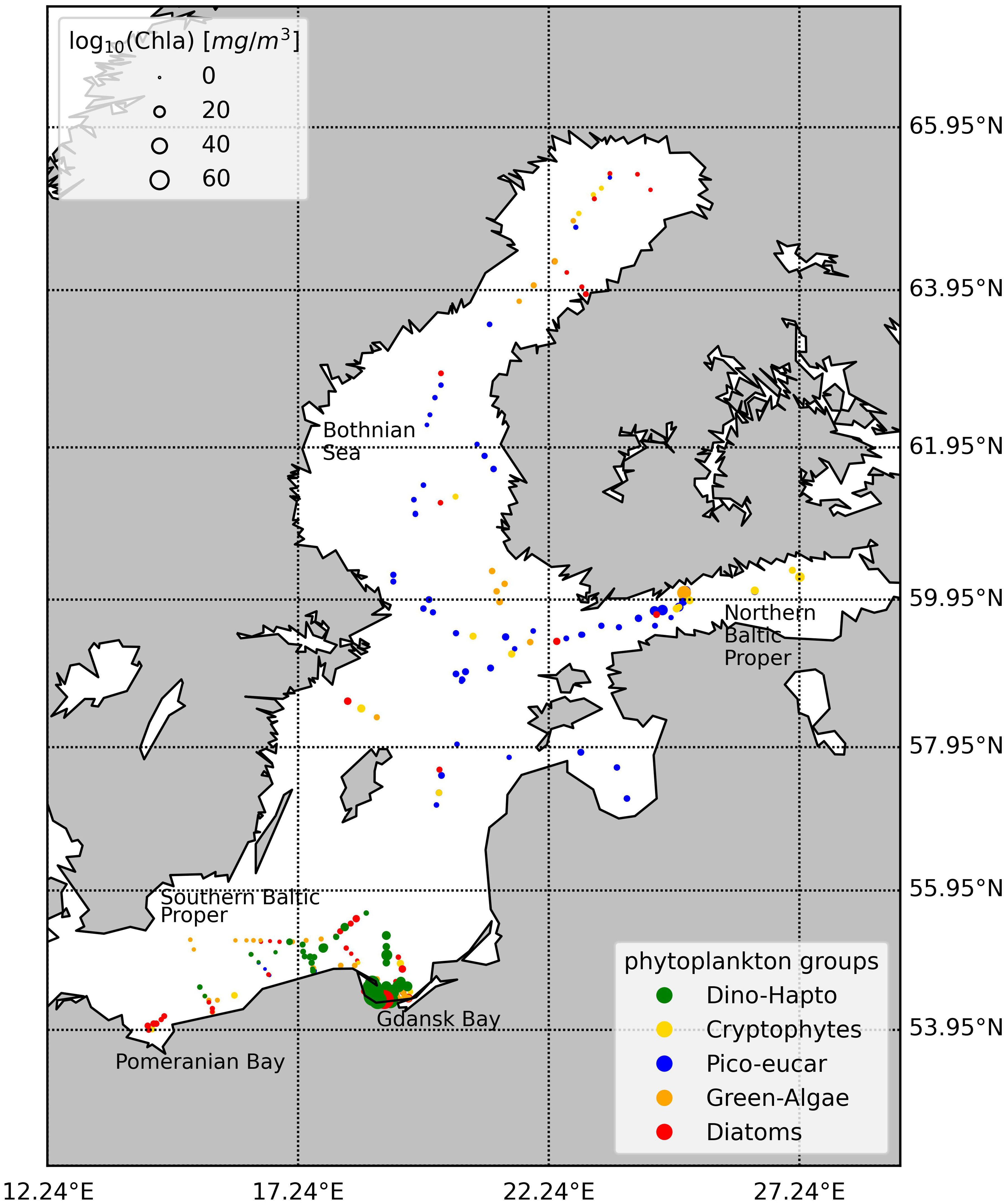
Figure 1. Spatial distribution of the sampling points in the years 2004-2008 color corresponds to dominant species present according to the network-community classification (NCA) in Canuti and Penna (2024).

The deployment of hyperspectral satellite such as the German Environmental Mapping and Analysis Program (EnMAP, Guanter et al., 2015) and the Italian Precursore IperSpettrale of Missione Applicativa (PRISMA, Candela et al., 2016) as well as the launch of the NASA Plankton, Aerosol, Cloud, ocean Ecosystem (PACE, Meister et al., 2024) mission, opens new possibilities for an integrated approach to phytoplankton studies. Several studies have focused on modeling or parameterizing light absorption by phytoplankton indirectly through diagnostic pigment analysis (DPA) and categorizing phytoplankton into phytoplankton functional types (PFT) and phytoplankton size classes (PSC) (Vidussi et al., 2001; Uitz et al., 2006, Brewin et al., 2010; Hirata et al., 2011; Mouw et al., 2017). IOCCG (2014) discusses various approaches to identify phytoplankton size structure from satellite data, and explores the potential for developing algorithms to remotely determine the contribution of different PFTs in water bodies. The use of biomarker pigments as representative of individual taxa, such as fucoxanthin (Fuco) for diatoms, has become a common method to infer phytoplankton community composition. However, this approach represents a simplification of the ecological and biochemical reality. While fuco is predominantly associated with diatoms, it is also present in other taxa such as haptophytes and some raphidophytes. This overlap limits the ability to accurately assign pigment concentrations to specific groups, thereby introducing potential biases and uncertainties into assessment of phytoplankton diversity and their use as proxies for individual taxa. Nevertheless, the PFT concept is relevant to the study of ecological and biogeochemical processes, particularly in model studies, as it helps to understand the role of phytoplankton in global cycles of key chemical elements and primary production. However, these methods are not effective for the Baltic Sea, which is an optically complex water body (Meler et al., 2020).

Due to significant freshwater inputs, the upper layer of the Baltic Sea contains a notable amount of chromophoric dissolved organic matter (CDOM), making CDOM absorption the dominant optical factor both in open water and along coastal regions. Particularly in the southern Baltic Sea, the inflow of large rivers contributes to increased optical variability (Harvey et al., 2015). CDOM is responsible for a significant fraction of the absorption of ultraviolet (UV) and blue spectral light in the ocean (Nelson and Siegel, 2013). Previous studies have explored the relationship between phytoplankton structure and CDOM content, correlating measurements of CDOM with phytoplankton composition (Barrón et al., 2014).

The phytoplankton absorption coefficient is a critical parameter in several applications, such as pigment biomass remote sensing or light attenuation in the ocean (Chase et al., 2013, 2017). The pattern of absorption spectrum is influenced by factors such as chlorophyll a concentration, algal species, cell size, and changes in pigment composition, including accessory pigments such as chlorophyll b and c, carotenoids, and phycobiliproteins. Similar to the chemotaxonomic characterization of Baltic Sea phytoplankton communities, which depends on diagnostic pigments (Schlüter et al., 2000; Stoń-Egiert and Ostrowska, 2022), the available models for retrieving phytoplankton biomarker pigments composition from absorption spectra for the Baltic Sea have focused on the southern Baltic Sea (Ficek et al., 2004; Kowalczuk et al., 2005). However, a significant research gap remains in the study of the wider Baltic basin. Additionally, most algorithms for interpreting remote sensing data in marine and oceanic environments are unsuitable for the Baltic Sea and lead to significant errors due to its unique characteristics (Meler et al., 2020).

This study aims to assess data analysis methods to investigate the relationship between phytoplankton pigment composition determined by high-performance liquid chromatography (HPLC) technique and optical properties throughout the Baltic Sea. The spectral dataset was subjected to different analysis techniques, including hierarchical cluster analysis (HCA) and principal component analysis (PCA). The results of the spectral analysis are compared with those of the corresponding phytoplankton pigment dataset studied previously (Canuti and Penna, 2024). Derivative analysis was applied to the pigmented absorption spectra dataset to obtain a predictive model for assessing the phytoplankton biomarker pigments from optical data. The proposed predictive model was then compared with the Gaussian spectral decomposition model (Hoepffner and Sathyendranath, 1991, 1993, Ficek et al., 2004; Chase et al., 2013) to evaluate the advantages and limitations of different approaches in a complex water basin such as the Baltic Sea.

2 Materials and methods

2.1 Field dataset

The dataset for the Baltic Sea was collected during six ocean color validation campaigns conducted in May and September 2004, April 2005, July 2006, August 2007, and August 2008. These campaigns focused primarily on the summer period, which is characterized by the dominance of filamentous cyanobacteria. However, they also included periods with low phytoplankton standing stock, typically from mid-May to mid-June, and the autumn diatom bloom. The first three campaigns covered the southern Baltic Sea, the Gulf of Gdansk, and the Pomeranian Bay, while the latter three campaigns focused on the northern Baltic Proper, the Gulf of Finland, and the Bothnian Sea (Figure 1). The complete Baltic Sea dataset (BA) comprises 273 stations.

Seasurface temperature (SST) and salinity were measured using the SBE 911 CTD (conductivity, temperature, depth) system (SeaBird, Alifax, USA). Water samples were collected at a surface depth of 1 m using a Niskin bottle and pre-filtered through a 150 μm mesh (Kartel, Germany). Filters for HPLC and spectrophotometric absorption measurements (GF/F filters, Φ 25 mm, 0.7 μm pore size, Whatmann, Germany) were pre-conditioned under constant mild vacuum (not exceeding 0.5 bar), flash-frozen in liquid nitrogen, and subsequently stored at -80°C. Additionally, 150 ml of water samples were filtered in the field (GSWP filters, Φ 47 mm, 0.22 μm pore size, Whatmann, Germany) and stored at 4°C in amber bottles until analysis.

2.2 Phytoplankton pigments dataset

Phytoplankton pigments were quantified at the Joint Research Centre of the European Commission (JRC) using the HPLC method described in Canuti (2023). The data set was subjected to quality control including participation in inter-laboratory exercises (Hooker et al., 2010; Canuti et al., 2016).

Of all the quantified pigments, those found below the detection limit in more than 95% of the stations were excluded from the study, as were redundant pigments (e.g., monovinyl chlorophyll already included in TChl a). The remaining eighteen pigments were the focus of the present study: 19’-hexanoyloxyfucoxanthin (Hex), 19’-butanoyloxyfucoxanthin (But), alloxanthin (Allo), Fuco, peridinin (Perid), diatoxanthin (Diato), diadinoxanthin (Diad), zeaxanthin (Zea), total chlorophyll b (TChl b), chlorophyll c1 + c2 (Chlc1c2), chlorophyll c3 (Chlc3), total chlorophyll c (TChl c), neoxanthin (Neo), violaxanthin (Viola), prasinoxanthin (Pras), lutein (Lut), α,β-carotene + β,β-carotene (Caro), and total chlorophyll a (TChl a). The composition of the total chlorophylls is described in Supplementary Table S1 (Supplementary Material). The photoprotective carotenoids, PPC, were defined as the sum of Caro, Zea, Allo, and Diad, while the phosynthetic carotenoid, PSC, was considered as the sum of Hex, Fuco, But and Peri.

In the use of phytoplankton pigments for categorizing phytoplankton into community and functional types, we referred to Supplementary Table S1, that was derived from Jeffrey et al. (1997); Seppälä (2009) and Roy et al. (2011).

2.3 Absorption coefficient dataset a_p(λ)

Similar to the HPLC analysis, the absorption coefficient, a_p(λ), was quantified at the JRC.

The method used to determine the absorption coefficient, a_p(λ), was a modified protocol of Tassan and Ferrari (1995). Transmittance–reflectance measurements were performed using a Perkin Elmer 950 (Perkin Elmer, USA) equipped with a 150 mm integrating spectralon sphere (Labsphere, USA). To calculate the absorption coefficients from the optical density, OD_s(λ), an appropriate correction must be applied to compensate for the elongation of the optical path due to multiple scattering in the material collected on the filter. This is achieved by using the dimensionless path length amplification factor, the β-factor, which converts the measured optical density of particles collected on the filter, OD_s(λ), to the optical density of these particles in solution, OD_sus(λ), (Mitchell, 1990) (Equation 1). The β-factor formula for the T-R method used in the present work is:

$\begin{array}{ll}O{D}_{sus}(\lambda )=0.719O{D}_s^{1.2287}& (1)\end{array}$

The coefficient of light absorption by all suspended particles was then calculated using the formula (Equation 2):

$\begin{array}{ll}{\text{a}}_{\text{p}}(\text{λ})=(\text{ln }(10)·O{D}_{sus}(\lambda ))/\text{l}& (2)\end{array}$

where l [m] is the hypothetical optical path in solution, determined as the ratio of the volume of filtered water to the effective area of the filter. The discrimination due to the pigmented, a_ph(λ), and the non-pigmented, a_NAP(λ), fractions of the particle absorption coefficient, is obtained by bleaching the sample on the filter by adding a solution of sodium hypochlorite (NaClO, Merck, Germany) as an oxidizing agent. The filter depigmentation is obtained by placing the filter horizontally against a filter holder (PALL, USA) and adding 1 mL of a 3.3% vol. of NaClO (4% active Cl) in Milli-Q water solution as a bleaching agent. In the original method, the distinction between the pigmented fraction, a_ph(λ), and the non-pigmented fraction, a_NAP(λ), of the particle absorption coefficient was monitored visually. In the modified protocol, the depigmentation process was monitored with a radiometer measurement (FieldSpec FS VNIR, Analytical Spectral Devices, USA) and a light source (Schott halogen fiber optic lamp, type 6423FO, Philips, Germany) between 300 and 1000 nm. The disappearance of the reflectance peak corresponding to TChl a at 675 nm was considered evidence of complete depigmentation. The bleaching process was monitored using the VNIR software (AnalyticalSpectral Devices, USA) (Canuti and van der Linde, 2006).

2.4 Chromophoric dissolved organic matter and suspended particulate matter dataset

Additionally, the dataset includes matched samples of suspended particulate matter (SPM) concentrations and the spectra of the light absorption coefficient of CDOM, a_g(λ). CDOM and SPM samples were analyzed at the JRC.

Concentrations of SPM [g m^-³] were determined by the gravimetric method combined with the loss-on-ignition technique. 47 mm GF/F filters were pre-combusted at 450°C for 4.5 h, rinsed in 1 liter of pure deionized water, and dried at 75°C for 2.5 h. After 4 hours in a desiccator, the filters were weighed and labeled using an analytical balance (Sartorius, Germany, precision 0.001 mg). In the field, depending on the concentration of suspended particles, 150 to 1500 mL of seawater was filtered through the filters, which were then rinsed with 30 mL of deionized water to remove surface salts and stored at -20°C until analysis. In the laboratory, the filters were thawed and dried at 75°C for 2.5 h, kept in a desiccator for 4 h, and then reweighed to determine the SPM value.

The a_g(λ), (m^-¹) measurement was carried out in the spectral range of 350 and 750 nm in a double beam double ray spectrophotometer (Perkin Elmer, USA), measuring the sample against double distilled water as a reference, using 100 mm optical path length quartz cuvettes. The optical density OD(λ) was converted to CDOM absorption by multiplying OD(λ) by 2.303 and then dividing by the path length l (m) (Mannino et al., 2019).

2.5 Methods in data analysis

2.5.1 Statistical analysis of the phytoplankton pigments dataset

The phytoplankton pigment dataset was subjected to statistical analysis to evaluate the pigment distribution in the different campaigns. In our previous study (Canuti and Penna, 2024), we applied a hierarchical clustering analysis (HCA) and a multivariate analysis (Principal Component Analysis, PCA), together with community partitioning by networkcommunity detection analysis (NCA), to the pigment dataset. These statistical analyses aimed to assess the phytoplankton community in the Baltic Sea in an alternative approach to widely used chemotaxonomic approaches, such as CHEMTAX (Mackey et al., 1996) or PFTs analysis. Here, the results of HCA and PCA applied to the pigments dataset were used in the organization and interpretation of the absorption coefficient dataset analysis.

2.5.2 Spectral decomposition of the absorption coefficient dataset

The spectral decomposition was applied with the aim of evaluating the agreement between our proposed predictive model (see section 2.5.4) and the Gaussian decomposition approach. To analyze the absorption coefficient, a_p(λ), dataset, we applied the Gaussian spectral decomposition proposed by Chase et al. (2013) and originally applied to AC-S (WetLabs, USA) data. The Chase et al. (2013) decomposition has shown a small residual error (0.001 m^-1), comparable to other Gaussian decompositions (Huping et al., 2019). In an attempt to use an algorithm not specialized for the southern Baltic Sea, we prefer the model of Chase et al. (2013) model to Ficek et al. (2004). In our study, we used the measured a_NAP(λ) value instead of approximating it with an exponential function, as in the original work of Chase et al. (2013). The initial wavelengths for the decomposition were those proposed by Chase et al. integrating the previous work of Hoepffner (1991, 1993) and Bricaud et al. (2004, 2007) (Table 1). To determine the optimal set of functions to approximate the decomposition, we used a leastsquares minimization (cost function, in Equation 3, Python3) to compare the reconstructed curve with the original curve:

Table 1

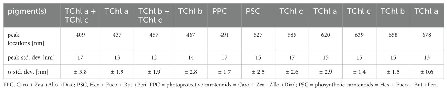
Table 1. Center wavelengths of Gaussian functions used for the spectral decomposition as in Chase et al. (2013).

$\begin{array}{ll}{\text{χ}}^2={\sum }_{\lambda =410}^{720}\frac{(a_p(\lambda )-({\sum }_{i=1}^{12} a_{gauss}({\lambda }_i)\left(\text{exp}\right\{-0.5{\left[\frac{\lambda -{\lambda }_i}{{\sigma }_i}\right]}^2\left\}\right)+a_{NAP}({\lambda }_i))}{{\sigma }_{SD}^2(\lambda )}& (3)\end{array}$

where a_p(λ), is the measured particle absorption, a_gauss(λ_i) is the magnitude of the i-Gaussian function, λ_i is the center wavelength of the i-Gaussian function, ${\sigma }_i$, is the width of the Gaussian. The equation is normalized by the standard deviation of the measured absorption spectra at each wavelength ${\sigma }_{SD}^2(\lambda )$. Following the approach of Chase et al. (2013), we identify correlations at specific wavelengths between HPLC pigments and Gaussian amplitude functions by checking the Spearman’s rank correlation coefficient. We then performed a linear regression analysis (least-square best fit) between the HPLC pigment concentration, assumed as a reference value, and the phytoplankton peak absorbance values, a_gauss(λ_i): the fit was calculated individually for each log-normalized pigment (pig_j) and absorbance peak according to the Equations 4 and 5:

$\begin{array}{ll}lo{g}_{10}(a_{gauss}({\lambda }_i))={\text{A}}_{ij}+B_{ij}*lo{g}_{10}(pi{g}_j)& (4)\end{array}$

The pigment concentration can be solved from the previous equation as:

$\begin{array}{ll}pi{g}_j={\{a_{gauss}({\lambda }_i)/exp*({\text{A}}_{ij})\}}^{1/B_{ij}}& (5)\end{array}$

A_ij and B_ij describe the relation between the jth pigment, pig_j, derived from the absorption spectra and the HPLC_j corresponding pigments.

2.5.3 Statistical and derivative analysis of absorption coefficient dataset

The correlation between a_ph(λ) (the absorption coefficient of pigmented particles) and changes in the phytoplankton community composition and abundance has been studied extensively (Bricaud et al., 2004, 2007, Chase et al., 2013). It is well known that the presence of different accessory pigments, such as diagnostic pigments found in different species, and differences among phytoplankton groups can influence the spectral characteristics of a_ph(λ) (Ciotti et al., 2002; Bricaud et al., 2004).

In our examination, we will consider both a_ph(λ) and the chlorophyll specific absorption coefficient of phytoplankton a*_ph(λ). The choice to also investigate a*_ph(λ) was based on the consideration that the package effect and the proportion of accessory pigment compositions are two major factors influencing the changes in the pattern and magnitude of a*_ph(λ). In addition, in the previous analysis of the HPLC pigment dataset, all the pigments were normalized against the ubiquitous TChl a. Consideration of a*_ph(λ) allowed us to compare the results of our derivative analysis and clustering more coherently with previous findings. We then considered the Pearson correlations (R) among spectral wavelengths, in particular those related to a_ph(λ), a_ph’(λ) and a_ph”(λ) (where the prime signs indicate the first and second spectral derivatives). We repeated the exercise for the a*_ph(λ), a*_ph’(λ) and a*_ph”(λ). Overall, we expected strong correlations among the pigment concentrations and the absorption spectra at all wavelengths, based on the previous findings by Catlett and Siegel (2018). Catlett observed significant multicollinearity problems in the analysis of the correlation between the pigments and a*_ph(λ), which could lead to an ill-conditioned model. To address this, a derivative transformation was applied to reduce the multicollinearity across different wavelengths.

Following the methodology outlined by Catlett and Siegel (2018) and Teng et al. (2022), we used derivative analysis to identify meaningful absorption characteristics and explore their associations with phytoplankton pigments and community structure. We focused on the spectral range between 400 and 750 nm, considering both the first derivative spectra, a_ph’(λ) and a*_ph’(λ) Equation 6, and the second derivative spectra, a_ph”(λ) and a*_ph”(λ) Equation 7:

$\begin{array}{ll}{a}_{ph}^{\text{'}}(\lambda )=\frac{a_{ph}(\lambda +\Delta \lambda )- a_{ph}(\lambda -\Delta \lambda )}{2*\Delta \lambda };a_{ph}^{\ast \text{'}}(\lambda )=\frac{a_{ph}^{*}(\lambda +\Delta \lambda )- a_{ph}^{*}(\lambda -\Delta \lambda )}{2*\Delta \lambda }& (6)\end{array}$

$\begin{array}{ll}{a}_{ph}^{\text{'}\text{'}}(\lambda )=\frac{a_{ph}(\lambda +\Delta \lambda )+a_{ph}(\lambda -\Delta \lambda )-2*a_{ph}(\lambda )}{\Delta {\lambda }^2};a_{ph}^{\ast \text{'}\text{'}}(\lambda )=\frac{a_{ph}^{*}(\lambda +\Delta \lambda )+a_{ph}^{*}(\lambda -\Delta \lambda )-2*a_{ph}^{*}(\lambda )}{\Delta {\lambda }^2}& (7)\end{array}$

We applied a finite band separation (i.e., $\Delta \lambda$) of 1 nm at the second order. To mitigate the effect of noise on our analysis, we implemented a noise reduction technique (Teng et al., 2022; Catlett and Siegel, 2018). In signal processing, we used the Savitzky-Golay filter to reduce signal noise and enhance the signal trend smoothness (Tsai and Philipot, 1998). This filter (Python3, svgolay) computed a polynomial fit for each running spectral window, employing a polynomial degree of 2 in our case and a window size of 15 nm. Before performing derivative analysis, we applied the smoothing filter to the spectral data to optimize the linear relationships between selected pigments and their respective absorption maxima, which were identified in the second derivative spectra.

2.5.4 Empirical orthogonal function model to assess pigment concentrations from optical measurements

We developed and evaluated a novel model to predict pigment concentrations in biological samples using the distinct correlation patterns observed between pigments and a_ph(λ), a_ph’(λ), a*_ph(λ) and a*_ph’(λ). Ideally, the model could be used to assess pigment concentrations from continuous optical measurements. To identify relevant features and reduce dimensionality, we used PCA for finding patterns in the data and transform them into a set of orthogonal variables called principal components. We will refer to this as an Empirical Orthogonal Function (EOF) model to avoid confusion with the PCA analysis of the HPLC pigment dataset.

The EOF analysis on the absorption dataset determines the wavelengths that most effectively capture the variance within the dataset. Here, we called X the absorption matrix, where each row (M) corresponds to an observation and each column (N) corresponds to a wavelength. The pigment dataset was represented by the matrix Y of dimensions MxP, where each row (M) represents an observation and each column (P) represents the concentration of pigments.

The matrix X was then subjected toa Singular Value Decomposition (SVD) to derive the EOF modes:

$\begin{array}{ll}\text{X=U}\Sigma V^T,{\text{ where x}}_{\text{ij}}={\displaystyle {\sum }_{k=l, N}{u}_{ik}{\sigma }_k{v}_{kj}}& (8)\end{array}$

In this equation, V is an N × N matrix containing the absorption data, U is an M × N matrix containing the principal components, Σ is an N × N matrix containing the singular values along the diagonal, and k represents the index of the EOF mode (with a length of N). We used a general linear model to forecast pigment concentrations (log-transformed), Equation 9 for each pigment, denoted as y_p. This model used a subset of principal components (PCs), represented as U, as covariates (Equation 8). We used both a_ph(λ) and a*_ph(λ) as well as a_ph’(λ) and a*_ph’(λ) PC decompositions, and in the case of a*_ph(λ) we also considered a linear regression with the non-log-transformed value of the pigments (Equation 10). The multiple regression model took the form:

$\begin{array}{ll}\text{log}({\text{y}}_{\text{p}})=\text{a}+{\text{b}}_1{\text{u}}_1+{\text{b}}_2{\text{u}}_2+\cdots +{\text{b}}_{\text{n}}{\text{u}}_{\text{n}}& (9)\end{array}$

$\begin{array}{ll}{\text{y}}_{\text{p}}=\text{c}+{\text{d}}_1{\text{u}}_1+{\text{d}}_2{\text{u}}_2+\cdots +{\text{d}}_{\text{n}}{\text{u}}_{\text{n}}& (10)\end{array}$

Here, log(y_p) represented the log(10) transformed concentration of pigment p, while u₁, u₂ … u_n represented the leading n PC scores of U. The model incorporated an intercept a and regression coefficients b₁, b₂,…, b_n. When the log-transformed pigment values were used as the target, a concentration of 0.00001 mg m^-³ was added to all values. When the non-log -transformed y_p concentration of pigment p, was used, the model intercept is denoted c and the regression coefficients d₁, d₂,…, d_n.

To define the subset of PCs, we excluded all those with standard deviations less than or equal to 0.0001 times the standard deviation of the first component. We then used multiple linear regression (MLR) to build predictive models using selected principal components. Stepwise feature selection, implemented through ordinary least squares (OLS) regression, facilitated the iterative inclusion and exclusion of features based on statistical significance. This process aimed to optimize model performance by selecting the most informative features, defining the number of n for each prediction. The selection of the best linear models was based on minimizing the Akaike Information Criterion (AIC). Once the optimal linear model was identified, the significance of the included terms was assessed by measuring the change in AIC (ΔAIC) when each term was removed.

Hence, we assumed that principal components explaining a larger proportion of the variability would be the first 100 principal components of a*_ph(λ) or of a’*_ph(λ), a_ph(λ) and a’_ph(λ), thus containing all the relevant information for modelling all pigments. To evaluate the robustness of this assumption, we performed cross-validation using 10, 25, 50, 100, and 200 principal components in the model formulation, respectively. The PCs with values too close to noise were excluded from the model. We tested this sensitivity using six distinct biomarker pigments: TChl b, Fuco, Peri, Allo, Zea and Peri. To evaluate the robustness and generalization of our models, we performed cross-validation with 500 permutations. This involved randomly splitting the data into training and test sets multiple times and calculating the Root Mean Squared Difference (RMSD) for each permutation. Scatter plots with logarithmic scales were generated to visualize the relationship between predicted and observed values, providing insight into the model’s predictive accuracy.

Metrics for the modelled a*_ph(λ), a’*_ph(λ), a_ph(λ) and a’_ph(λ), such as the coefficient of determination (R²), root mean square difference (RMSD), slope (S) and intercept (a) of the linear regression were derived from the log predicted values, log(y_p^P), compared to the log observed pigment concentration data, log(y_p). Conversely, metrics a such as mean percent difference (MPD), percent bias (PB), and median percent difference (MDPD) were always computed based on non-log-transformed pigment concentrations.

$\begin{array}{ll}\mathrm{RMSD}=\sqrt{\frac{1}{N}{\displaystyle {\sum }_{i=1}^N{[\log (y_p^P)-\log (y_p)]}^2}}& (11)\end{array}$

$\begin{array}{ll}MPD=\frac{100}{N}{\displaystyle {\sum }_{i=1}^N[(y_p^p-y_p)/y_p]}& (12)\end{array}$

$\begin{array}{ll}\text{MDPD}=median(100 \frac{(y_{i,p}^P-y_{i,p}^V)}{y_{i,p}^V})& (13)\end{array}$

Where $y_{i,p}^V$ is the observed pigment concentration for observation i, $y_{i,p}^P$ is the predicted pigment concentration for observation i and N is the number of observations.

In evaluating the models, we performed cross-validations with 500 permutations to rigorously assess their performance. This process involved iteratively partitioning the dataset into training (X_train) and (X_val) test subsets to endure robustness in model evaluation. In the first approach, the data was randomly split into two subsets, with 80% of the data used for model fitting/training, including X_train, and the remaining 20% was used for prediction validation, including X_val. In the second approach, we isolated a specific campaign as the training dataset and fine-tuned the method on the remaining data. From each permutation, we calculated the RMSD and its variation coefficient, providing insight into the prediction accuracy and consistency across different data splits.

To gain a visual understanding of model performance, we generated scatter plots with logarithmic scales. These plots allowed us to observe the relationship between predicted and original values, providing a graphical representation of the model’s predictive ability. Additionally, regression lines, representing the relationship between predicted and observed values were superimposed on the scatterplots. These lines were accompanied by R-squared values, providing a quantitative measure of the goodness of fit of the models.

3 Results

3.1 Variability and clustering of the dataset

Our dataset was examined in terms of variability. The key statistical data highlighting the variability within our dataset are summarized in Table 2; Figure 2 (Table 2; Figure 2). It is noteworthy that the yellow substance shows a high variation in the whole dataset. The range of TChl a varies from a concentration typical of oligotrophic water (0.272 mg m^-3) to concentration characteristic of eutrophic conditions (60.222 mg m^-3). In our dataset, Peri, the diagnostic pigment representing the dinoflagellate community, exhibited the highest range of concentration variation: the range was from the instrumental limit of detection to 21.395 mg m^-3 reached in the BA03 campaign (Supplementary Material, Table S2). The salinity varies from 7.83 to 1.70 PSU. The maximum and minimum values were recorded in the BA03 campaign (Southern Baltic), while for the other campaigns the salinity value was always higher than 2.3 PSU (Supplementary Material, Table S2). The concentrations of Hex, But, Peri, and Zea contained several null values, which may later affect the model, as the computation was based on few measurements. It is important to point out that a dataset with such extreme variability (where key features have a CV greater than 100%) can make it difficult to build a stable model. This level of variability can lead to an ill-conditioned model, where small changes in the input data cause large, unpredictable changes in the output, reducing reliability and accuracy of the model.

Table 2

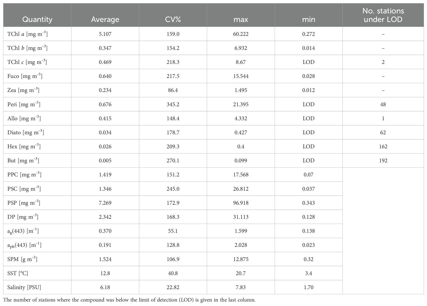
Table 2. Summary statistics for the entire data set: the pigments and the pigments sum concentrations and the spectral at specific absorption (a_g(443), a_ph(443)), coefficient of variation (CV%), mean and range (max-min).

Figure 2

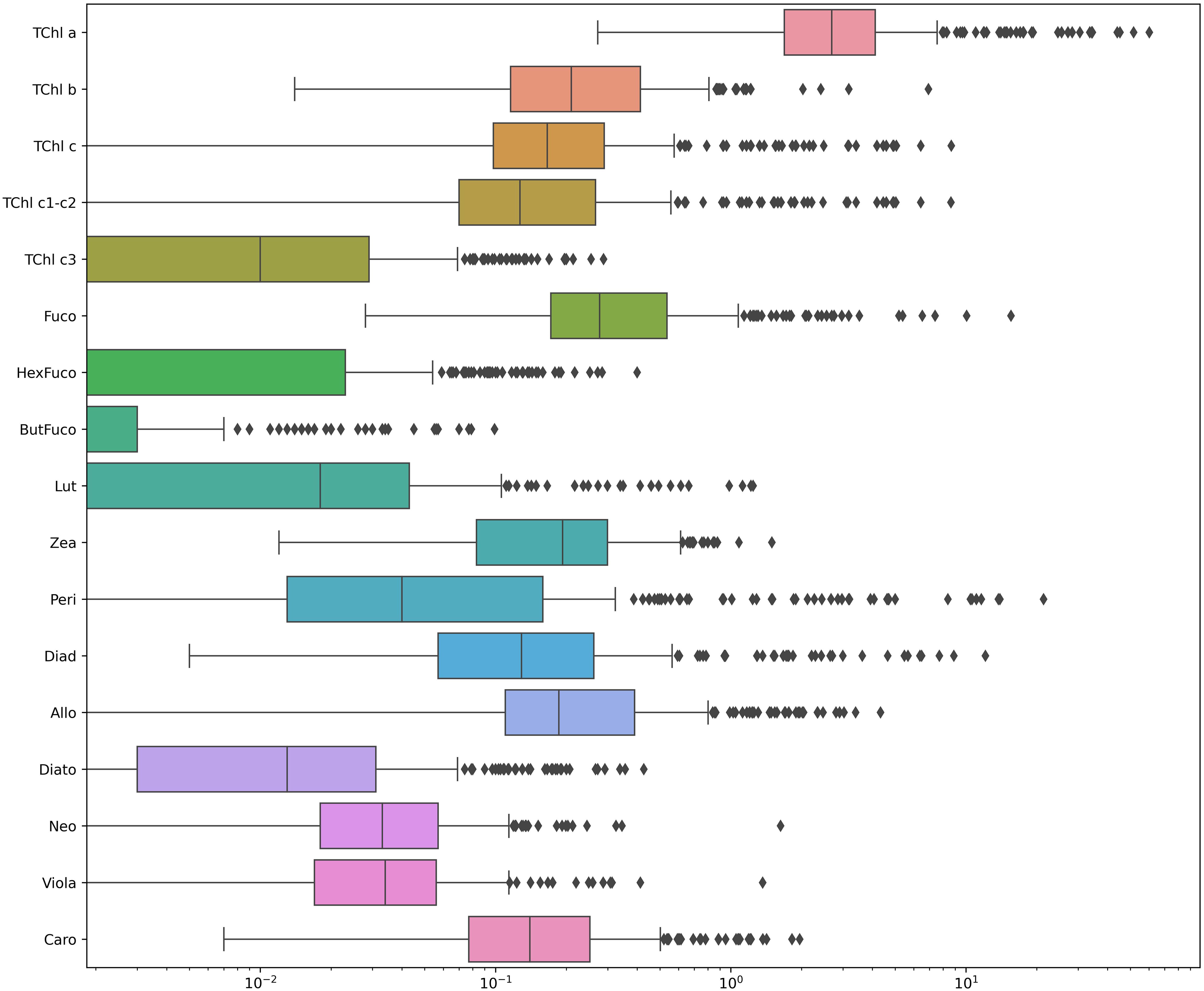
Figure 2. Boxplot of pigment concentrations in the Baltic Sea on a logarithmic scale. Each box represents the distribution of pigment concentrations (mg m^-3) measured across sampling stations. The x-axis uses a log₁₀ scale to highlight differences in magnitude among pigments. Outliers are displayed as individual points beyond the whiskers.

We considered the different contributions to light absorption at 412 and 443 nm from detritus, CDOM and plankton and their relation with environmental variable: temperature and salinity (Figure 3). All stations showed a relevant light absorption (higher than 60%) from the dissolved organic matter. The light absorption by phytoplankton, a_ph was less than 50% for most of the points: the highest relative absorption was found in the BA03 campaign in the southern Baltic Sea in April (Supplementary Material, Table S2). The largest contribution to the total light absorption was made by CDOM: 52% ± 20%. a_g is more dominant in the Bothnian Sea (BA06), where the ternary plot shows a strong clustering toward the CDOM-rich end, consistent with high terrestrial input from surrounding rivers, while the contribution of a_NAP was the lowest (less than 20% for all the stations) (Supplementary Material, Table S2). In contrast, the southern Baltic (BA01-BA03) exhibits a more balanced distribution among phytoplankton a_ph, a_g and detrital material a_NAP, reflecting a more mixed optical regime with a significant phytoplankton contribution. The Gulf of Finland and the Northern Baltic Proper (BA4, BA5) show higher variability, likely driven by episodic riverine inputs and hydrodynamic mixing events. The environmental conditions further support these findings. The inverse relationship between salinity and a_g confirms that CDOM originates primarily from terrestrial sources, with the highest concentrations found in the low-salinity waters of the Bothnian Sea and Gulf of Finland while the Southern Baltic shows lower a_g values at higher salinity (~6-7 PSU), indicating more marine-influenced waters with less terrestrial CDOM input. Phytoplankton absorption a_ph, on the other hand, follows seasonal trends, with higher values occurring in cooler waters during the spring months (BA01, BA03), indicative of phytoplankton blooms. Late summer campaigns (BA02, BA05) show a shift toward higher CDOM absorption, likely due to increased riverine discharge and organic matter degradation. The spectral dependency of optical properties, evident in the shifts from 412 nm to 443 nm, suggests variability in phytoplankton composition and CDOM characteristics. The ternary plot patterns align with these trends, as campaigns with high a_ph, correspond to periods of active phytoplankton growth, while those with dominant a_g reflect enhanced CDOM inputs. Overall, the separation of data points across different campaigns underscores the diverse optical regimes within the Baltic Sea, shaped by riverine influence, seasonal biological productivity, and basin-specific hydrodynamic conditions.

Figure 3

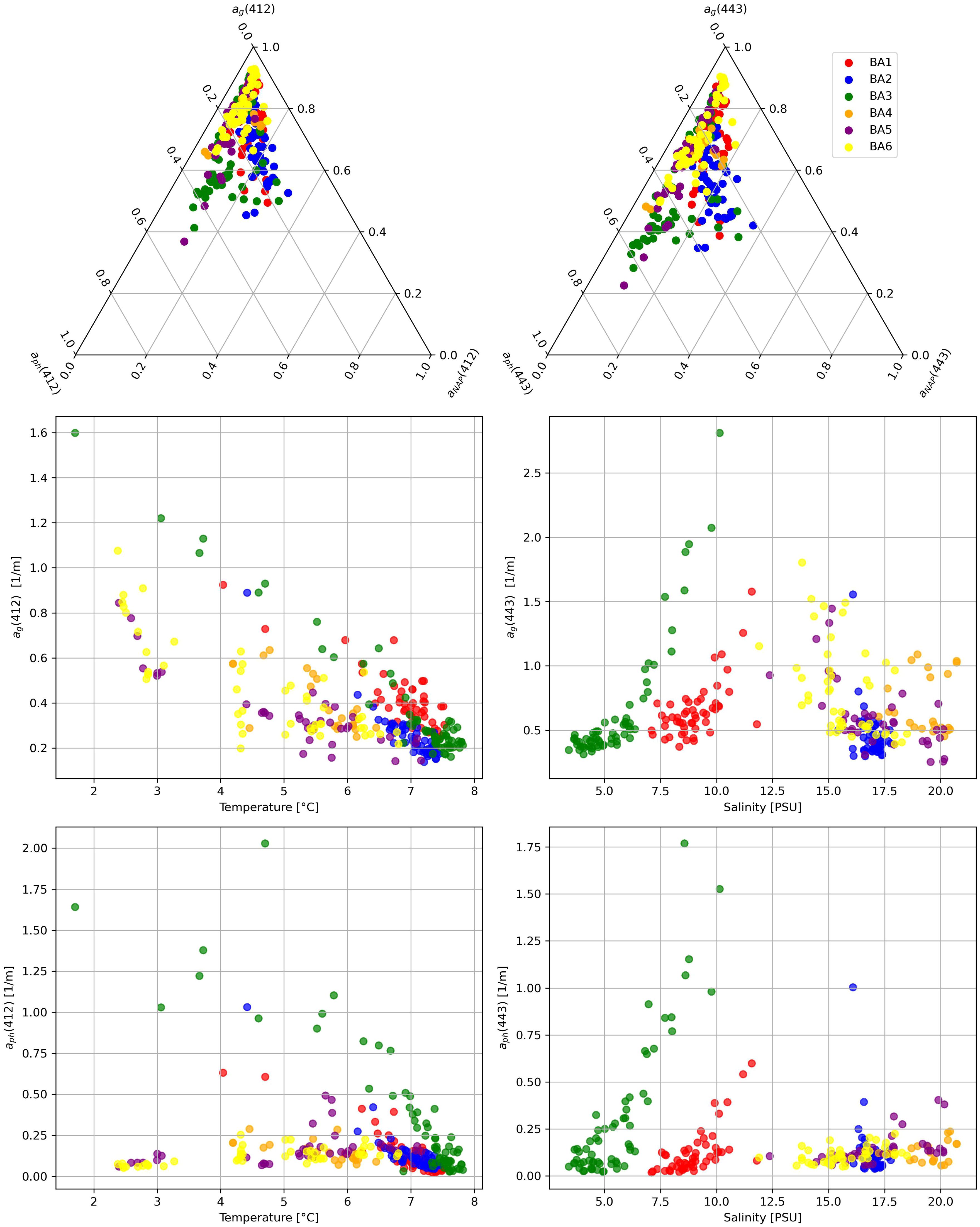
Figure 3. Multivariate analysis of absorption properties a_g, a_ph and a_NAP at 412 nm and 443 nm and in relation to environmental parameters (temperature and salinity). Top row: Ternary plots showing the relative contributions of different absorption coefficients. Middle and bottom rows: Scatter plots illustrating the variations in absorption coefficients as functions of temperature and salinity across different oceanographic campaigns (BA1–BA6).

Both methods, HCA and PCA analyses, were used to analyze the relationships between different pigments across various phytoplankton groups, highlighting distinct subgroups and their correlations (Figure 4). The HCA analysis of the Baltic (BA) pigment dataset (HCA_pig) identified five distinct phytoplankton pigment groups. Marker pigments helped to identify specific phytoplankton groups. The orange cluster (haptophytes, nanoflagellates) included pigments such as Hex, TChl c3, Pras, and Diad, which are typically found in haptophytes and nano-sized phytoplankton. Pigments such as Allo, Caro, and Lut fell into the Green Cluster (green algae, dinophytes, cryptophytes) representing a mix of pigments found in green algae, dinophytes, and cryptophytes. The presence of peri, often specific to dinophytes, strengthened the grouping of this taxonomic class. The red cluster (micro/pico, diatoms, eukaryotic/cyanobacteria) consisted of the pigments Fuco, TChl b, and Zea, indicating different phytoplankton size classes, with Fuco representing diatoms, and Zea and TChl b representing picoeukaryotes. PCA on the normalized phytoplankton pigment concentrations highlighted spatiotemporal variations in the BA dataset. The four leading PCA modes together explained 67.4% of the variability. Mode 1 showed a strong positive correlation with dinoflagellates and cryptophytes, and a negative correlation with green algae and cyanobacteria. Mode 2 correlated positively with diatoms and haptophytes, while Mode 3 had strong correlations with green algae and nanofraction pigments. Mode 4 discriminated diatoms from other groups, especially in the Gulf of Finland. The PCA results recalled some aspects of the HCA, such as the dominance of diatoms in certain campaigns. The HCA_pig was shown here to see how well it matched the clustering of the absorption spectra (HCA_spectra).

Figure 4

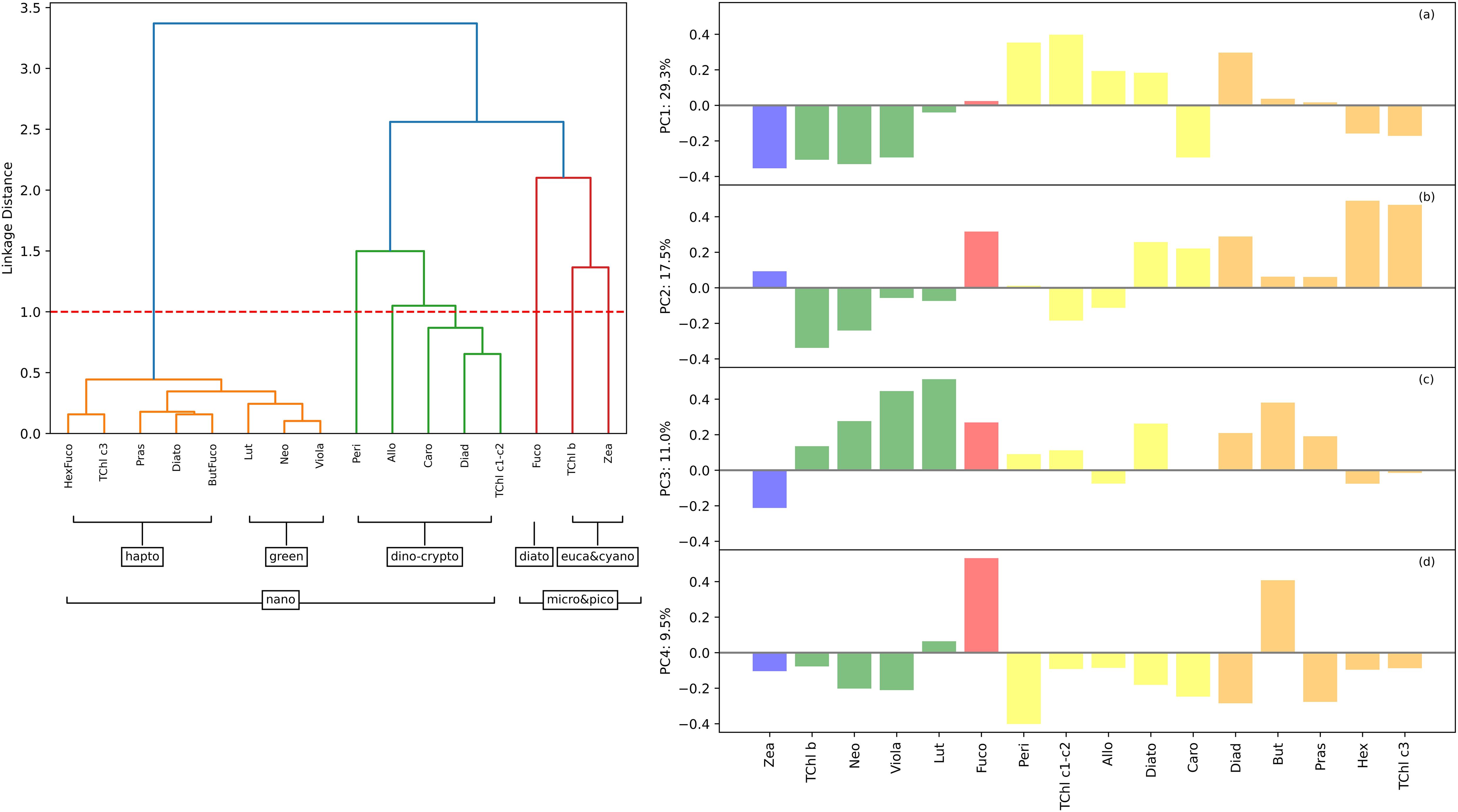
Figure 4. HCA_pig dendrogram (left) and PCA biplots (right) of phytoplankton pigment ratios to TChl a for the Baltic dataset. In the HCA_pig (left figure), the major pigment communities (micro-, nano- and pico-phytoplankton) were identified based on a linkage distance cutoff of 1.0 (red dashed line). The proposed phytoplankton cell size classes for each group are shown in brackets. In the right figure, the loadings corresponding to the principal component (PC) modes are shown in panels (a-d) for the Baltic dataset. The pigment order was the same as in the HCA analysis, to facilitate comparison. The mode number was shown above each plot, together with the percentage of variance explained by that mode. The loadings were color coded according to the main taxonomic groups: blue for cyanobacteria-pico, red for diatoms-micro, orange for green algae-nano, green for haptophytes-dinoflagellates-nano, and orange for euglanophytes-nano.

3.2 Spectral decomposition of the phytoplankton absorbance

The spectral decomposition approach gave a reliable representation of the pigment composition (Chase et al., 2013; Hoepffner and Sathyendranath, 1991, 1993, Ficek et al., 2004), however, it presented the limit of omitting some DPA pigments without considering carotenoids and xanthophylls individually. The omitted pigments included Peri, Allo and Zea that were the DPA of a representative phytoplankton population commonly found in the Baltic ecosystem. In our dataset, the Gaussian decomposition of a_ph at the selected wavelengths (Table 1) produced residuals within ± 0.001 m^-¹ for all stations (Figure 5), confirming its robustness for most pigments. The pigments were correlated with different a_gauss as in Chase et al. (2013). The linear regression emphasized the relationship between pigment concentrations and their absorption characteristics for the selected wavelengths (Figure 6): strong linear fit indicated that Gaussian decomposition estimated well the pigment.

Figure 5

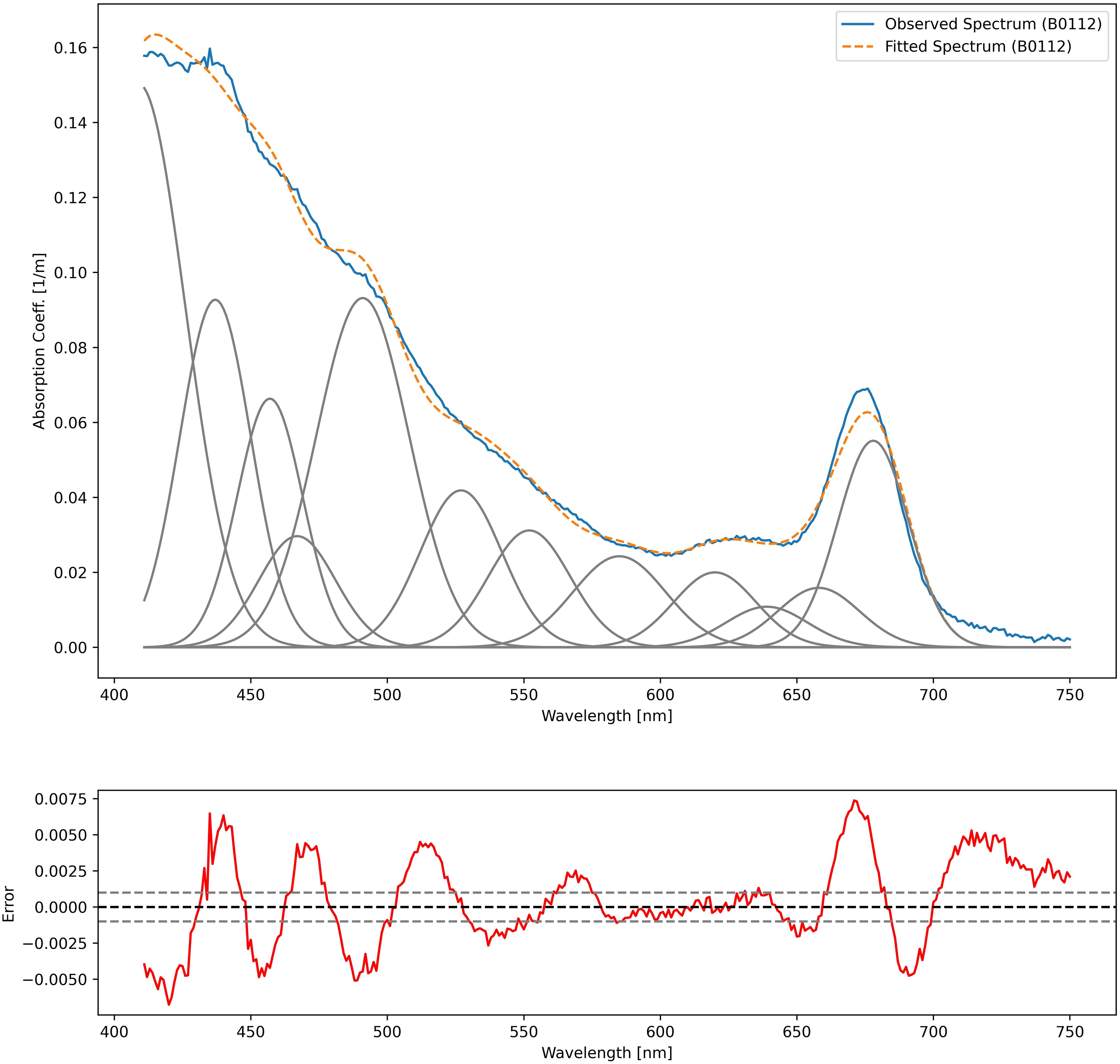
Figure 5. Observed absorption spectra (in blue), best Gaussian fitting (in grey) and the fitted curves (in orange dashed lines) for the BA01_12 station, and (bottom plot) the residual between observed and fitted spectra (in red).

Figure 6

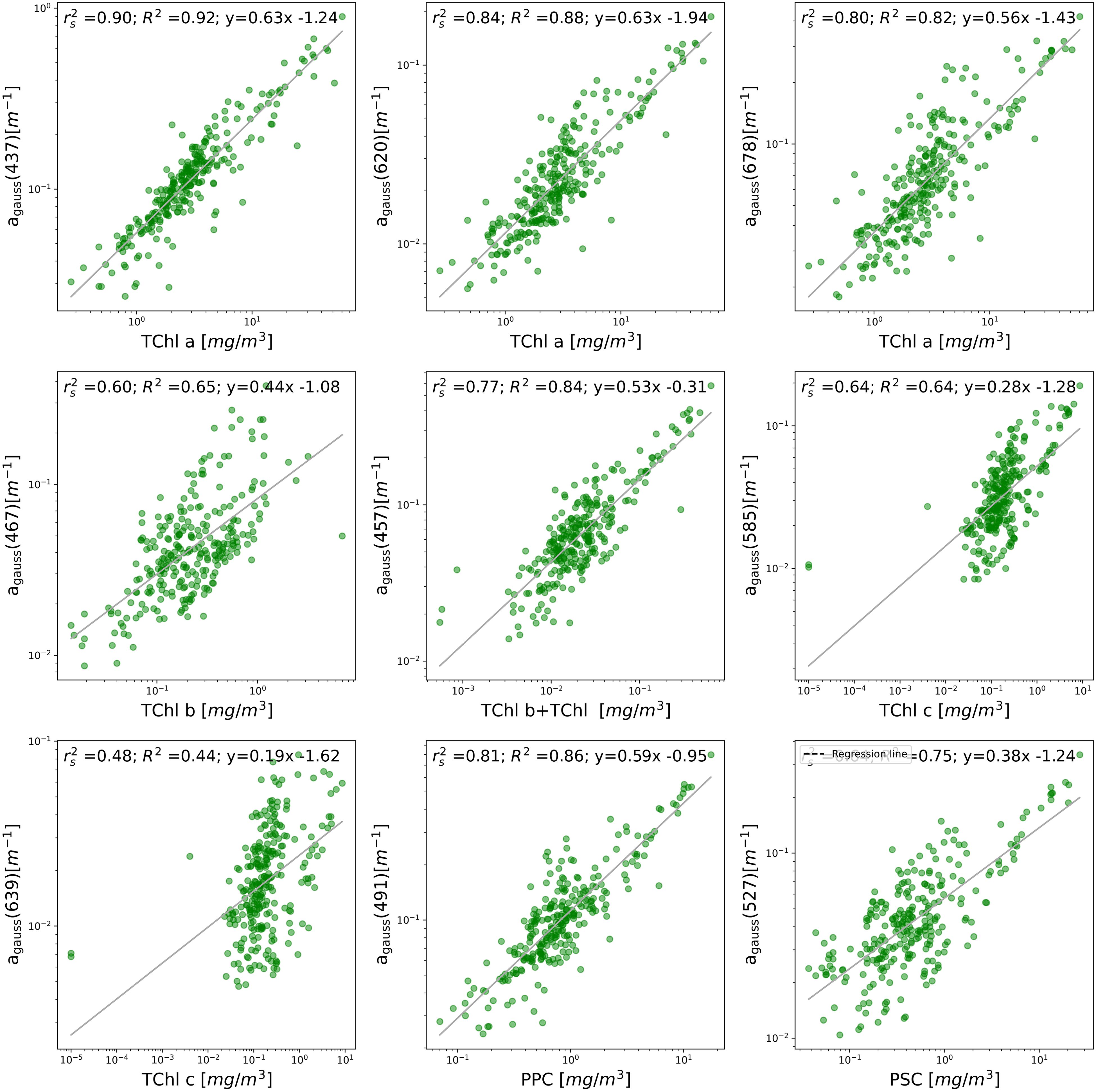
Figure 6. HPLC-measured chlorophyll, photoprotective carotenoids (PPC) and photosynthetic carotenoids (PSC) concentrations (on the y-axis) compared to the magnitudes of Gaussian peak absorption (on the x-axis) at eight distinct wavelengths. The continuous line represents the best-fit linear regression on the logarithmic transformations of both datasets.

The Table 3 reported Spearman’s rank correlation coefficients (r^2s) and correlation coefficients R² along with the coefficients A and B determined by the Equation 4 described in section 2.5.2. The coefficients A_ij and B_ij describe the relation between the j-th pigment, pig_j, derived from the absorption spectra and the HPLC_j corresponding pigments, providing insight into the effectiveness of our model in predicting pigment concentrations. The Gaussian decomposition at wavelengths 437 nm and 620 nm, show high correlation with TChl a obtained by HPLC: we obtained a r^2s of 0.90 and an R² values of 0.92 between for the a_gauss at 437 nm and TChl a and we had r^2s of 0.84 and R² of 0.88 for a_gauss 620 nm and TChl a. These correlations indicated a strong relationship between HPLC concentrations and optical measurements at these wavelengths. At 678 nm, the correlation of TChl a and a_gauss was slightly lower but still substantial, with r^2s of 0.80 and R² of 0.82. For TChl b, we considered the a_gauss at 467 and 557 nm: the correlation was weaker with respect what we had with TChl a. TChl b exhibited an r^2s values of 0.60 at 467 nm and 0.77 at 557 nm, and R² values of 0.65 and 0.84, respectively. At 557 nm The sum of TChl b and TChl c showed a better correlation with the a_gauss than TChl b alone (Table 3). TChl c had r^2s values of 0.64 (R² = 0.64) at a_gauss 585 nm and of r^2s of 0.48 (R² = 0.44), at a_gauss 639 nm, showing moderate correlations. For the pigments PPC and PSC, the correlations were relatively strong with r^2s values of 0.81 and 0.64 and R² values of 0.86 and 0.75, respectively. The coefficients A and B vary, indicating different degrees of sensitivity and offset in the correlation. Regarding the aggregated pigments, the photoprotective carotenoids (PPC) correlated better (0.81) than the photosynthetic carotenoids (PSC, 0.64), i.e. in the range of TChl b. It should be noticed that the PSC included the fuco, a pigment that was ubiquitous present in the dataset.

Table 3

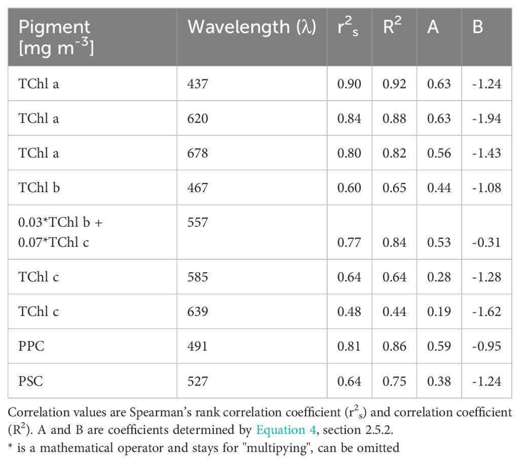
Table 3. Correlations between HPLC pigment concentrations at ten different a_gauss wavelengths.

3.3 Correlation of phytoplankton pigments with CDOM and absorption spectra

Correlation analyses were carried out to determine the associations between the data series of each inherent optical property (IOP) and the first four amplitude functions (AFs) representing various phytoplankton communities, as determined by PCA analysis of the HPLC pigment datasets. The AF values were used as proxies for these communities. The inclusion of different optical properties in our analysis provided a more comprehensive understanding of the relationships between pigments and optical properties. Correlations with CDOM absorption values were computed for the first four modes (Figure 7). Modes 1 and 4, associated with dinoflagellates and diatoms, showed positive associations with a_g(λ). Conversely, the other modes did not show significant correlations with a_g(λ). The a_ph(λ) correlation with the PCA results was significant in the case of the first mode, i.e. the mode associated with predominantly dinoflagellates. The AFs included in the analysis are derived from the analysis of the pigment to TChl a ratio.

Figure 7

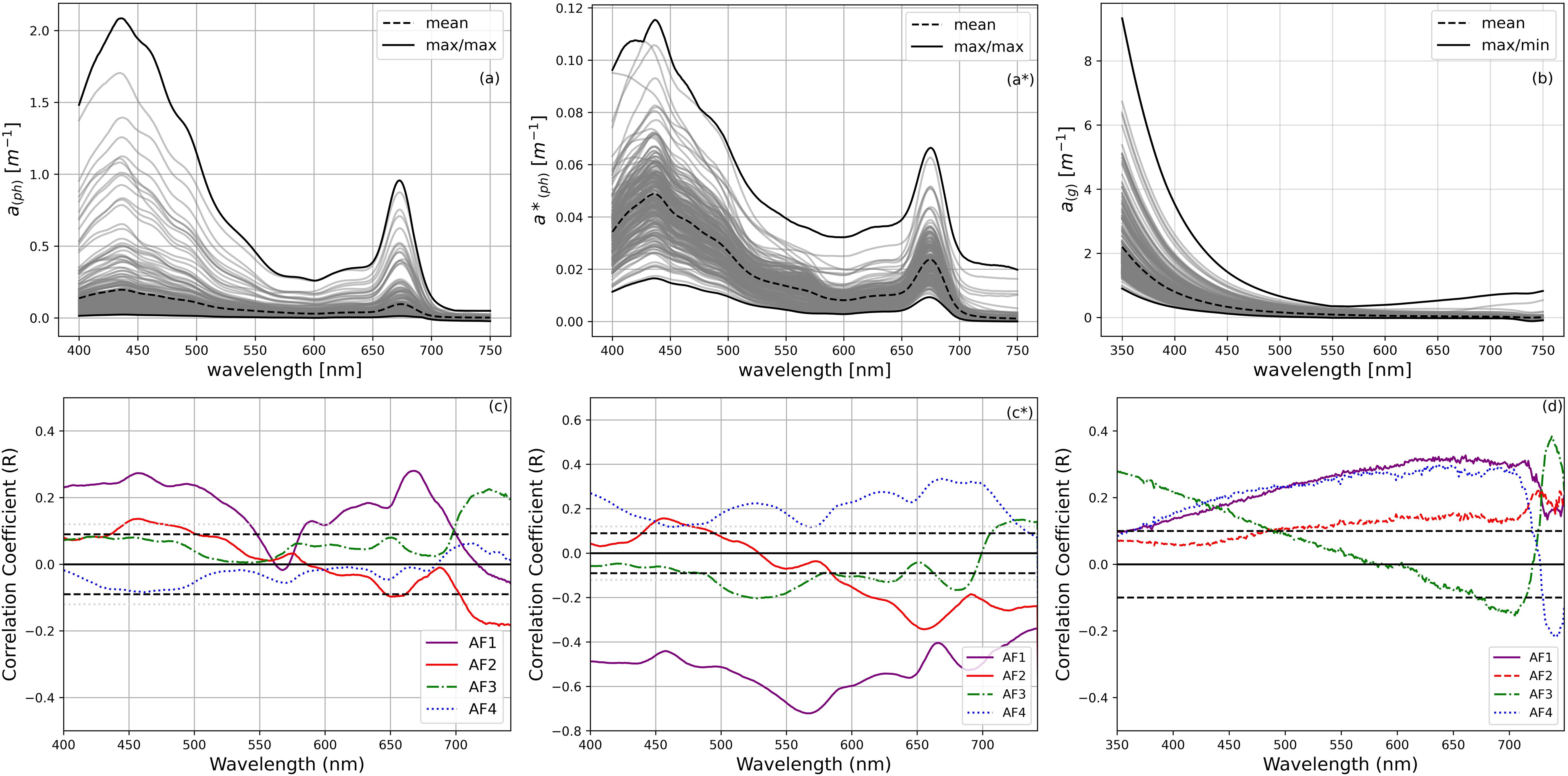
Figure 7. Average absorption properties and their correlation with the first four modes derived from the PCA analysis for (a, c) phytoplankton absorption, a_ph(λ); (a’, c’) phytoplankton absorption ratio to TChl a, a*_ph(λ); (b, d) CDOM absorption, a_g(λ). In c, c’ and d the 95% confidence interval (CI) is shown by the black dashed line.

Further insights were gained by analyzing a_ph’(λ) and a_ph”(λ), and the distinct spectral relationships between the concentrations of selected biomarker pigments and values within specific wavelength intervals (Figure 8) . The same exercise was repeated for the a*_ph’(λ) and a*_ph”(λ) (Figure 9). The pigments were grouped into the following categories based on the outcomes of the HCA_pig analysis: (a, e) dinoflagellates, (b, f) chlorophytes, (e, f) haptophytes, and (d, h) diatoms and picoplankton. It is noteworthy that Lut and Diato were omitted – for clarity in the representation-, although they showed analogous patterns to the chlorophytes (b, f) and haptophytes pigments, respectively.

Figure 8

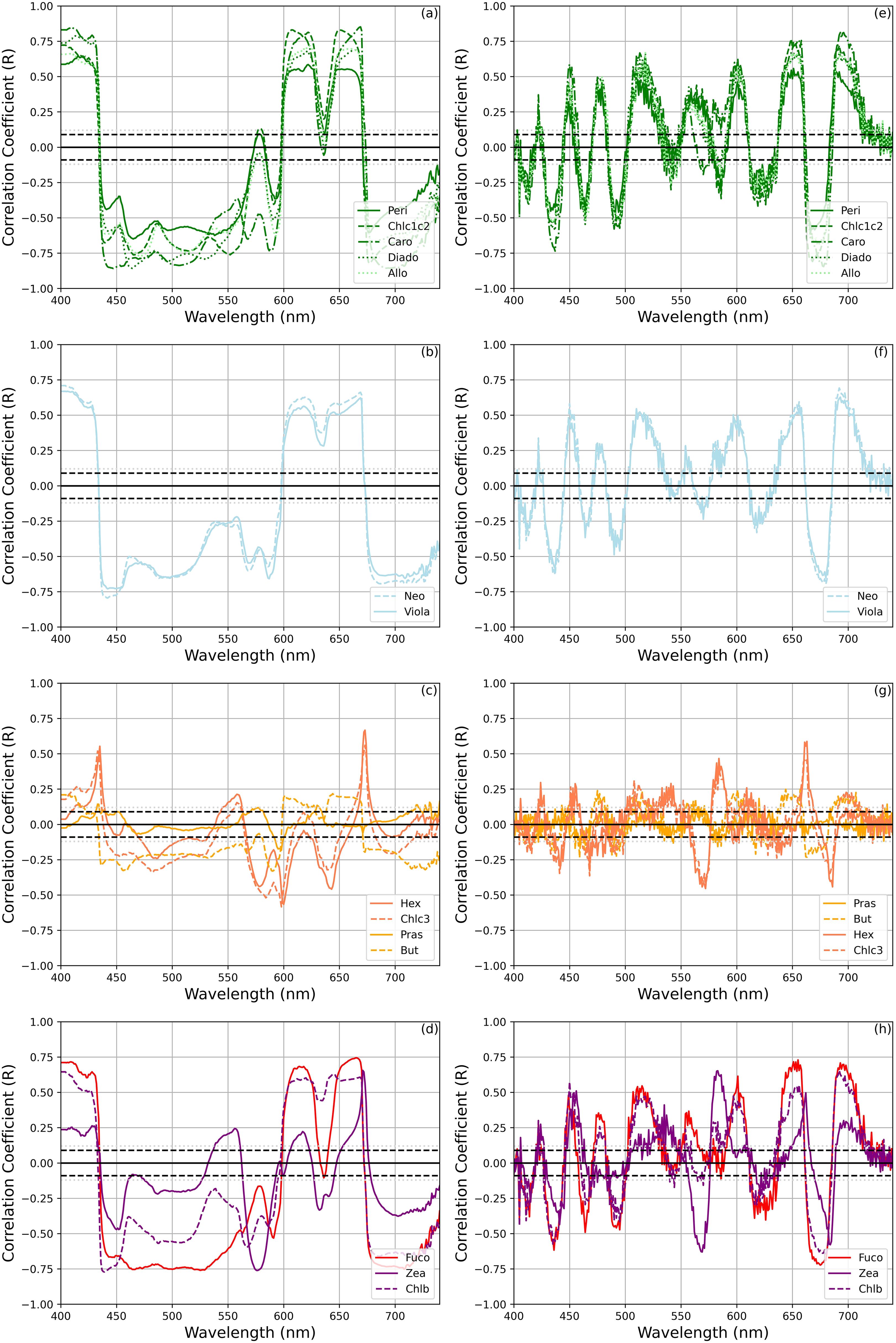
Figure 8. Correlations of selected phytoplankton pigments with a_ph^’(λ) and a_ph^”(λ) grouped as the results of the HCA_pig analysis ((a–d) for a_ph^’(λ) and (e–h) for a_ph^”(λ)). The dashed and dotted black lines indicate the magnitude of the significant correlation coefficients at 95% and 99% confidence, respectively.

Figure 9

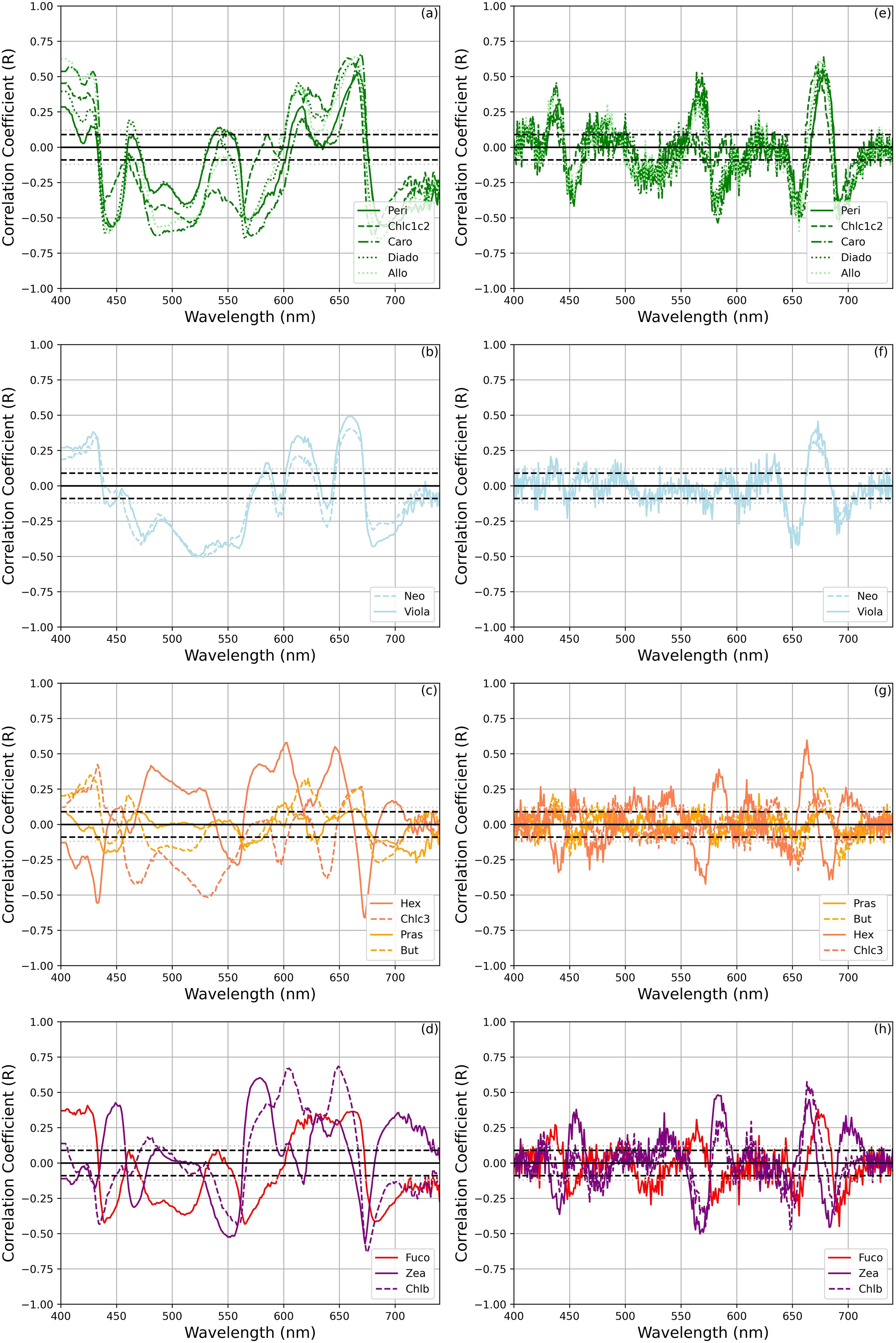
Figure 9. Correlations of selected phytoplankton pigments with a*_ph^’(λ) and a*_ph^”(λ) group as the results of the HCA_pig analysis [(a–d) for a*_ph^’(λ) and (e–h) a*_ph^”(λ)]. The dashed and dotted black lines show the magnitude of significant correlation coefficients at 95% and 99% confidence, respectively.

The HCA spectra clustering analysis was conducted to explore the relationships between pigment concentrations and spectral absorption features across different wavelength intervals. Using Ward’s HCA and Euclidean distance, the clustering was applied to the first and second derivatives of the phytoplankton absorption coefficients (a_ph^’(λ) and a_ph^”(λ)) collectively referred to as HCA_spectra (Supplementary Material, Figure S1). This approach allowed for the identification of distinct clusters that represent groups of pigments based on their spectral behavior. To maintain consistency with the HCA_pig results, a distance threshold of 5 was used, producing four clusters for both a_ph^’(λ) and a_ph^”(λ). The HCA_spectra resulting clusters showed that Fuco grouped with Allo, Peri, and Caro, despite Fuco forming a distinct cluster in the pigment-based HCA_pig, analysis. The overall clustering pattern highlighted consistent pigment distributions, particularly in the largest cluster, between the first and second derivatives. The number of clusters obtained for HCA_spectra was four for both a_ph^’(λ) and a_ph^”(λ), and the pigment distribution among the biggest cluster was consistent between a_ph^’(λ) and a_ph^”(λ). In Figure 10 we reported the correlation between the pigments and the spectra following the clusters obtained from the HCA_spectra analysis for a_ph^’(λ) and a_ph^”(λ). We repeated the exercise for the a*_ph(λ) and in Figure 11 we reported the correlation between the pigments and the spectra following the clusters obtained from the HCA_spectra analysis for a*_ph^’(λ) and *a_ph^”(λ): the number of clusters obtained in these case were five for the first derivative, and three for the second derivative.

Figure 10

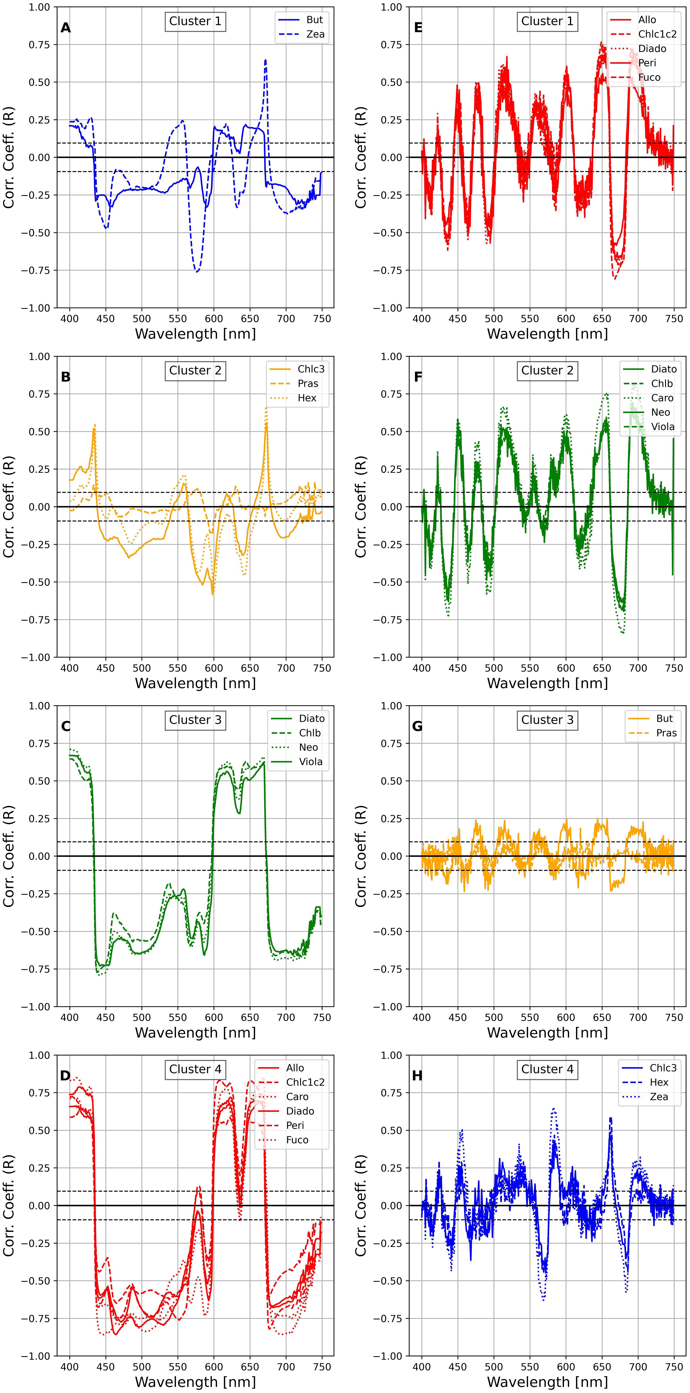
Figure 10. Correlations of selected phytoplankton pigments with a_ph^’(λ) and a_ph^”(λ) grouped as the results of the HCA_spectra ((A–D) for a_ph^’(λ) and (E–H) for a_ph^”(λ)). The dashed and dotted black lines show the magnitude of the significant correlation coefficients at 95% and 99% confidence, respectively.

Figure 11

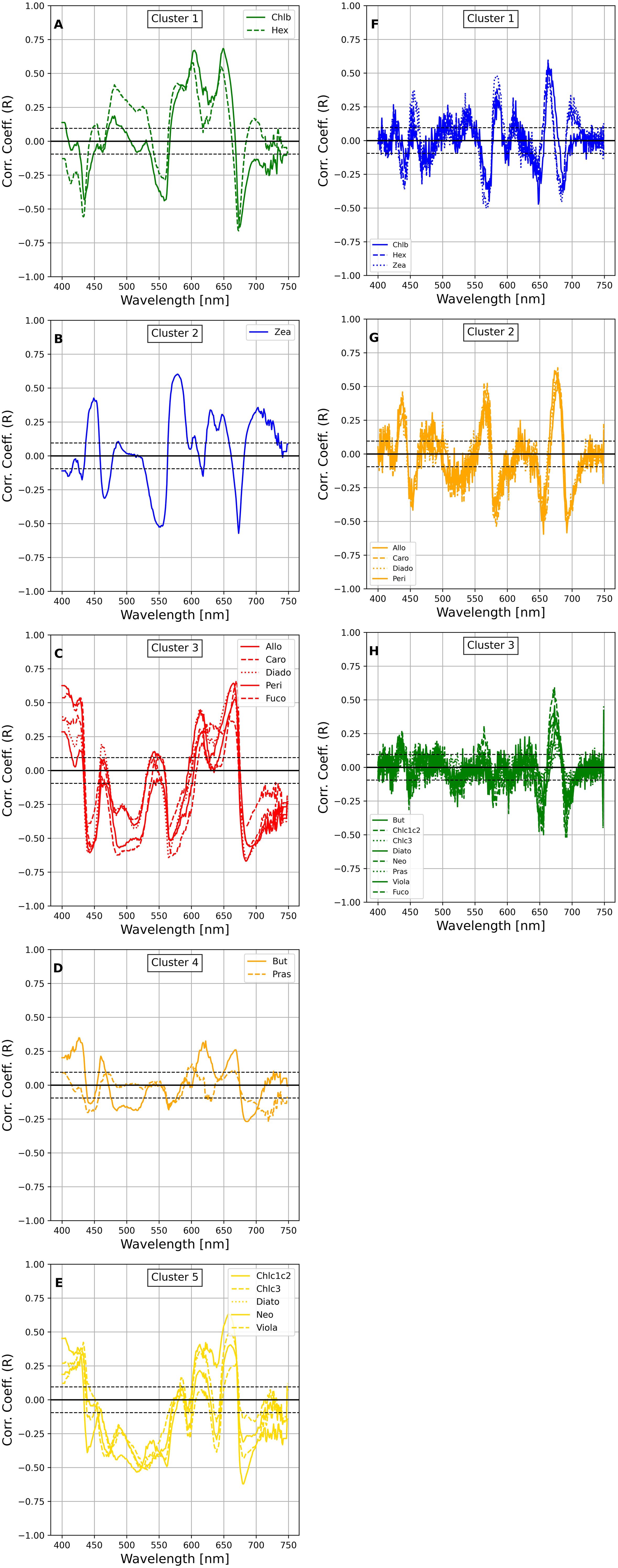
Figure 11. Correlations of selected phytoplankton pigments with a*_ph^’(λ) and a*_ph^”(λ) group as the results of the HCA_spectra [(A–E) for a*_ph^’(λ))and (F–H) for a*_ph^”(λ)]. The dashed and dotted black lines show the magnitude of significant correlation coefficients at 95% and 99% confidence, respectively.

3.4 Proposed EOF-model to assess pigment concentrations from optical measurements

The purpose of this study was to develop a model for phytoplankton pigment concentrations based on spectra derived from the absorption coefficient, with the aim of assessing pigment levels by optical measurements using characteristic correlation patterns between pigments and a_ph(λ). We tested a_ph(λ), a’_ph(λ), a*_ph(λ) and a*_ph’(λ) versus pigment concentrations and log-transformed concentrations. The pigments included in the analysis were all the DPA: Peri, Allo, Fuco, Zea, TChl b, TChl c1c2 and Hex. These pigments were the bio-markers that were associated with specific phytoplankton groups and commonly used in phytoplankton pigments analysis. The performance metrics for MLR models predicting pigment concentrations using PC regression with the first 100 PCs were shown (Table 4). The optical metrics evaluated included a_ph(λ), a_ph’(λ) and a*_ph’(λ), with metrics comprising the coefficient of determination (R²), RMSD, and RMSD coefficient of variation (RMSD CV%) from cross-validation with 500 permutations. Fuco models performed differently for different metrics. The a_ph(λ) model achieved an R² of 0.645 with an RMSD mean of 0.3 and an RMSD CV% of 11, indicating moderate accuracy and consistent performance. Improved results were seen with the a_ph’(λ) model, which had an R² of 0.739 with similar RMSD mean and CV% values. However, the a*_ph’(λ) model showed slightly lower performance with an R² of 0.47 and the highest RMSD CV%. For Zea, the a_ph(λ))model showed an R² of 0.391, an RMSD mean of 1.1, and an RMSD CV% of 7.4, reflecting lower accuracy and variability. The a_ph’(λ) model offered a modest improvement with an R² of 0.45, and similar RMSD mean and CV% values. The a*_ph’(λ) model achieved an R² of 0.45, showing modest performance. For Allo, the a_ph(λ) model had an R² of 0.541 with an RMSD mean of 0.4 and a higher RMSD CV% of 25. The a_ph’(λ) model improved to an R² of 0.56 but also had a higher RMSD CV%. In contrast, the a*_ph’(λ) model had a lower R² of 0.38, an RMSD mean of 0.23, and a significant RMSD CV% of 43.15, indicating considerable variability. The TChl b models showed good performance. The a_ph(λ) model had an R² of 0.716, with an RMSD mean of 0.3 and an RMSD CV% of 20.5. The a_ph’(λ) model showed similar efficacy with an R² of 0.714. The a*_ph’(λ) model performed best with an R² of 0.79, the lowest RMSD mean, and CV%, indicating superior predictive accuracy. For Hex, the a_ph(λ) model achieved an R² of 0.624 with an RMSD mean of 0.9 and an RMSD CV% of 9.8. The a_ph’(λ) model had a slightly lower R² of 0.603 with similar RMSD mean and CV% values. The a*_ph’(λ) model showed improved performance with an R² of 0.67, better RMSD mean, and CV%, reflecting improved accuracy. The Peri models varied, with a_ph(λ) yielding an R² of 0.44, an RMSD mean of 1, and an RMSD CV% of 8.3. The a_ph’(λ) model had similar R² and RMSD mean, with a slightly higher RMSD CV%. The a*_ph’(λ) model had an R² of 0.47, a lower RMSD mean but a higher CV%, indicating variable performance. The TChl c1c2 models were particularly effective. The a_ph(λ) model had an R² of 0.58, an RMSD mean of 0.4, and a higher RMSD CV% of 31.5. The a_ph’(λ) model performed similarly performance with a slightly better mean RMSD. The a*_ph’(λ) model stood out with an R² of 0.87, the lowest RMSD mean, and CV%, reflecting superior predictive ability. Finally, the a_ph(λ) model for But showed lower performance with an R² of 0.36, an RMSD mean of 0.8, and an RMSD CV% of 8.1. The a_ph’(λ) model had comparable R² and RMSD mean, with a slight increase in RMSD CV%. The a*_ph’(λ) model was less effective, with an R² of 0.27, a higher RMSD mean, and a low RMSD CV%. Overall, the models showed variable performance for different pigments and optical metrics. The highest accuracy and lowest variability were observed for TChl c1+c2 using a*_ph’(λ), while pigments such as Zea and But showed lower prediction accuracy. These findings highlight the importance of selecting appropriate principal components and optical metrics to optimize model performance in predicting pigment concentrations.

Table 4

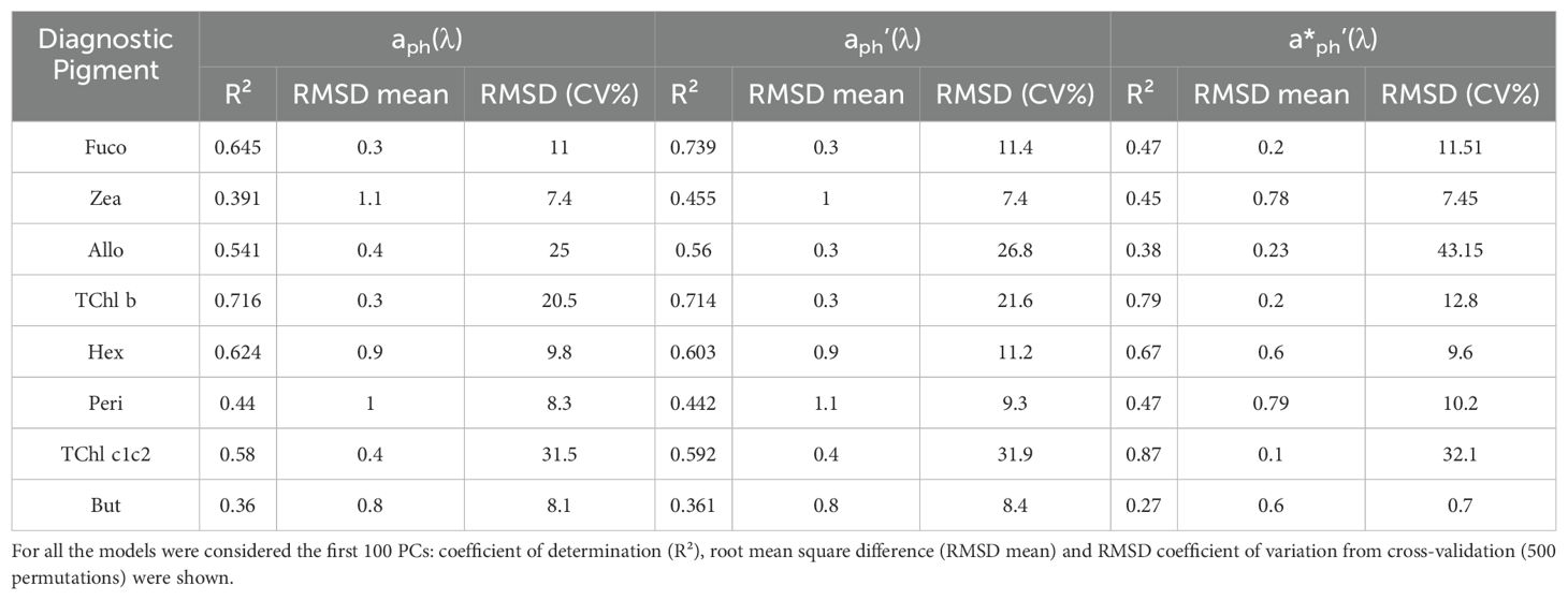
Table 4. Diagnostic pigments MLR model for PCs regression of a_ph(λ), a_ph’(λ) and a*_ph’(λ).

In the Baltic Sea, the chlorophyll c is not representative of any phytoplankton community, while Allo, Fuco, Zea and TChl b are. Based on this consideration, the most promising outcomes were achieved when using a_ph’(λ) and using log-transformed pigment concentration as the target (see Figure 12). It is worth noting that the model showed better performance in the southern Baltic Sea, as demonstrated during validation with the isolation of a specific campaign (data not shown here). The model derived from a_ph’(λ) performed better than from a*_ph’(λ) both for the Fuco (0.`74 against 0.47) and the Allo (0.56 against 0.38) and closely for Zea (0.45 in both models) and TChl b (0.71 and 0.79), while the model with a*_ph’(λ) had a better regression for the TChl c1c2 (0.87 vs 0.59 for the a_ph’(λ) model).

Figure 12

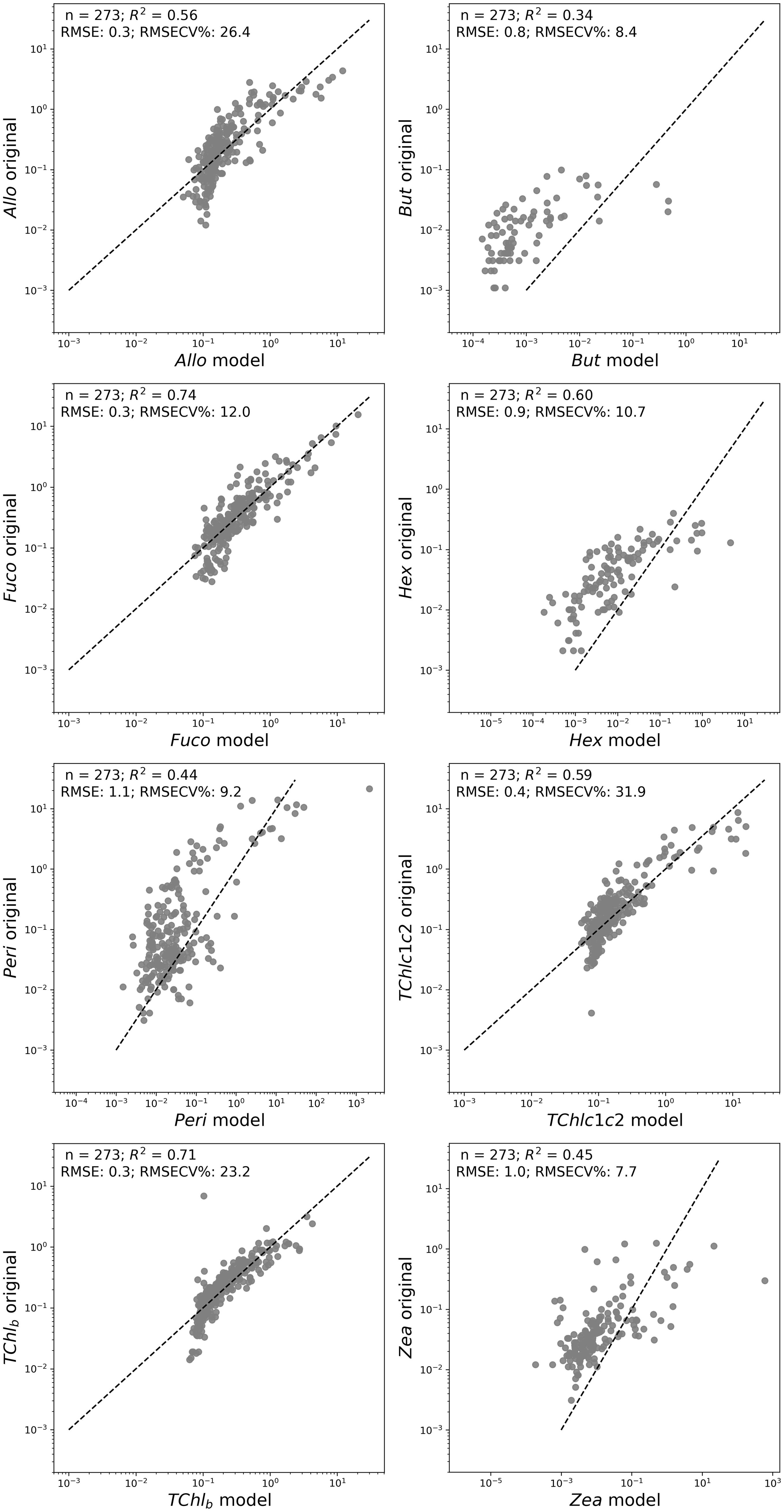
Figure 12. Scatterplots of original data against the model in logarithmic scales for the MLR based on a_ph’(λ) PCs for diagnostic pigments. The equations of regression lines, along with R-squared values, were shown.

While the Gaussian decomposition detected TChl b absorption primarily at 658 nm and 457 nm, our model identified additional significant correlations for TChl b at 440 nm, 600 nm, and 660 nm. These results suggest that our approach, using a_ph’(λ) and its first derivatives, captures a broader spectral representation of TChl b absorption. Similarly, for TChl c, Gaussian decomposition highlighted peaks at 415 nm, 430 nm, 480 nm, and 665 nm, but our model found important correlations at additional wavelengths, particularly around 575-590 nm and 600 nm, broadening the understanding of TChl c’s spectral absorption.

A variability for Allo demonstrated correlation coefficients across the visible spectrum (Figure 13). Significant correlations were seen in the 450-500 nm and 600-650 nm wavelength ranges, as indicated by the narrowing of the 95% confidence intervals (CI). These regions likely corresponded to absorption peaks associated with the carotenoid structure of Allo suggesting that these wavelengths are essential for accurate prediction Allo concentrations. The narrow confidence intervals in these areas reinforced the model’s consistency in capturing the relevant spectral signals. In the case of But, correlation coefficients hovered close to zero across most of the spectrum, with minor dips in the 450-550 nm range. The wide C.I. reflected significant uncertainty in these predictions, indicating that the absorption features of But were either weakly represented in the a_ph’(λ) -based model or confounded by signals from other pigments. This result showed the poor performance for But (see Figure 12), with an R² of 0.34.

Figure 13

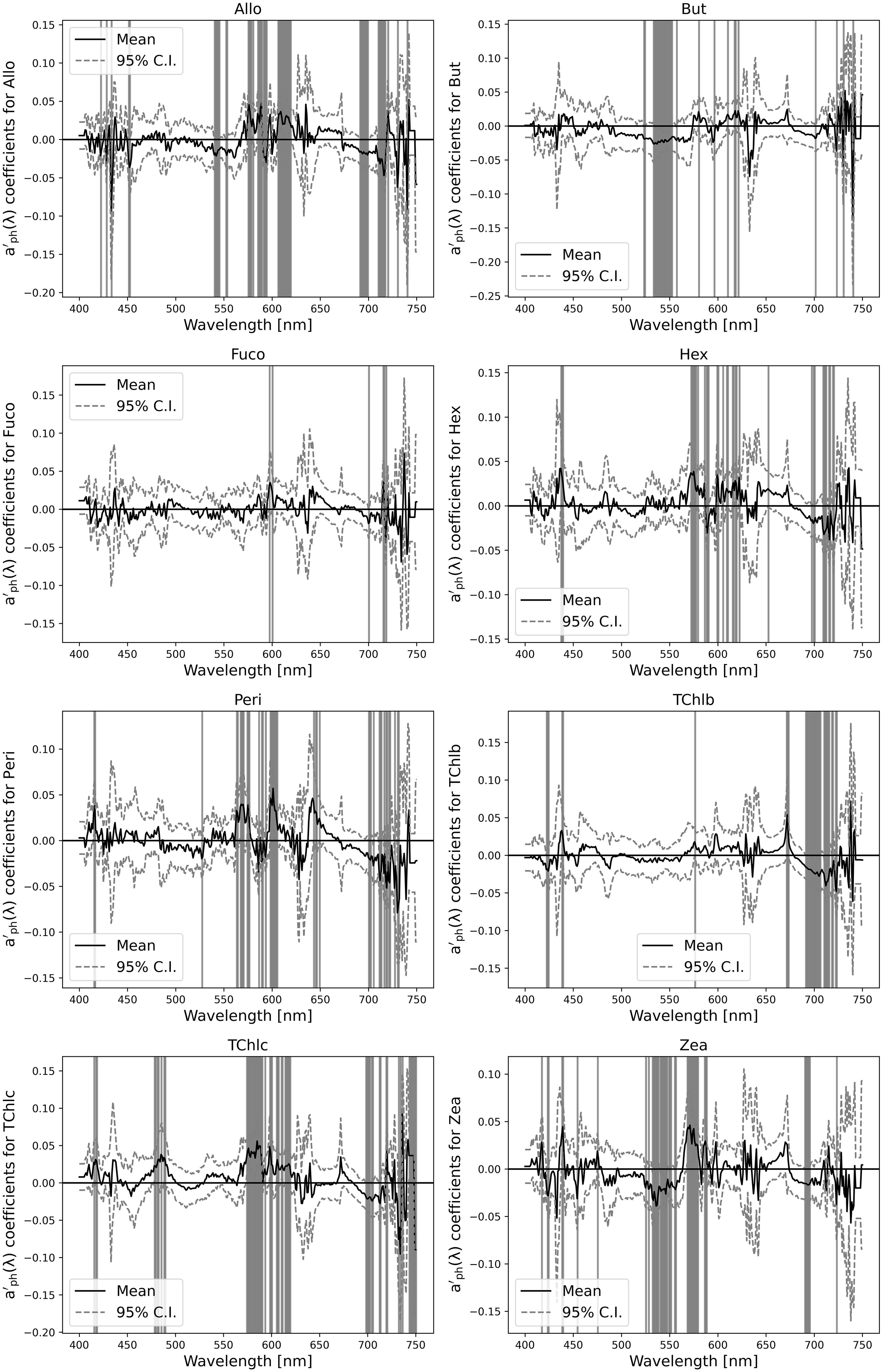
Figure 13. Correlation coefficient between the model based on the first derivative of the absorption coefficient a_ph’(λ) and individual pigment concentrations across different wavelengths.

For Fuco, stronger correlations emerged, especially in the 500-550 nm and 620-680 nm ranges, which matched the known absorption features of Fuco. The tight C.I. around these wavelengths suggested high model confidence in predicting Fuco concentrations. The strong response at around 540 nm, a significant Fuco absorption peak, underlined the significant influence of pigment on the high performance of the model (R² = 0.74). Hex showed similar trend to But, with minimal correlation across the spectrum, small peaks in the 400-450 nm range and slight variations around 650-700 nm suggesting some wavelength influence. However, the wide C.I. and relatively flat response indicate that the model struggles to predict Hex accurately, consistent with the lower R² (0.60). This suggested that the absorption signature of Hex was not well captured by the a_ph’(λ)-based model. For Peri, notable correlation peaks appeared in the 450-500 nm and 650-700 nm regions, corresponding to Peri’s characteristic carotenoid absorption in the blue-green spectrum. These peaks were accompanied by narrower confidence intervals, indicating a reliable model fit in these bands. However, the model’s overall predictive accuracy was moderate (R² = 0.44), and broader variability suggested some difficulty in isolating Peri’s signal from others, leading to a higher RMSD (1.1). TChl b exhibited strong correlations in the red region (600-700 nm), particularly around 650-675 nm, where chlorophyll b had its key absorption peak. The model’s high performance for TChl b (R² = 0.71) was reflected in the narrow confidence intervals at these wavelengths, indicating their importance in accurately predicting TChl b concentrations. Minor peaks also appeared in the 450-500 nm region, reflecting additional absorption by TChl b in the blue range. For TChl c, the correlation plot showed scattered peaks, particularly around 450-500 nm and 650-700 nm, which matched with the absorption features of TChl c. However, the broader, more variable confidence intervals suggested a lower level of confidence in these predictions, probably due to overlapping signals from other pigments. This was consistent with the moderate performance for TChl c (R² = 0.59). Finally, Zea showed a flatter correlation pattern, with weak but noticeable peaks in the 450-500 nm range and a less distinct response in the 600-650 nm region. The broad C.I. suggested high uncertainty, consistent with the low R² value (0.45) in Figure 12. This indicates that Zea’s absorption characteristics were difficult to distinguish, contributing to the challenges in modeling Zea concentrations accurately.

4 Discussion

The present study examined the surface phytoplankton community distribution in the Baltic Sea, derived from IOPs and HPLC datasets covering different seasons and different areas of the Baltic Sea.

The high variations in these results were in agreement with the findings on previous pigments and absorption dataset analysis representative of the Southern Baltic (Woźniak et al., 2022; Meler et al., 2018, 2020). The variability expressed as coefficients of variation (CV%, defined as the ratio of the standard deviation to the average value) in Meler et al. (2020) was of 163% for the TChl a (here 159%) and of 137% for a_ph at 440 nm (here of 128.8% for a_ph at 443 nm). Notably, the yellow substance exhibits high variation throughout all the dataset, in agreement with the finding of Harvey et al. (2015). Meler et al. (2023) in a study dedicated to the Southern Baltic and the Gulf of Gandsk found that the average contribution of a_ph was 29% ± 14%, while for the detritus it was 19% ± 9% and, in agreement with our findings, the greatest contribution to the total light absorption was made by CDOM: 52% ± 20%.

Our data-driven statistical analyses on the absorption coefficient dataset identified distinct taxonomically defined phytoplankton communities in the Baltic Sea, characterized by five biomarker pigments: diatoms (Fuco), dinoflagellates (Peri), cryptophytes (Allo), green algae (TChl b) and cyanobacteria-pico-plankton (Zea). As already addressed in the introduction to this study, the use of biomarker pigments as representative of single taxa (i.e., Fuco for the Diatoms, while Fuco contributes to different taxa) is a simplification.

The unsupervised statistical techniques used in the data analysis were applied to both the HPLC pigment dataset and the absorption coefficient dataset. The analysis of the CDOM coefficient showed that the a_g(λ) attributed to non-living particles was found to be consistently more pronounced when microplankton groups dominated the phytoplankton community, as observed in Modes 1 and 4. This finding was consistent with previous observations (Barrón et al., 2014). This can be explained by the higher production of detrital organic matter by larger microplankton, such as diatoms and dinoflagellates, which tend to have shorter life cycles and faster sinking rates, leading to an accumulation of non-living organic particles in the water column. These particles contributed to the CDOM pool and enhance the a_g(λ) signal. For Modes 2 and 3 corresponding to the phytoplankton community composition with a predominant nanoplankton fraction, there were no significant correlations observed at any wavelength. This suggested that there were no significant relationships between the non-living portion of the absorption spectrum during periods when nanoplankton were dominant. Smaller phytoplankton, such as cyanobacteria and haptophytes, generally have slower sinking rates and lower production of particulate organic matter, resulting in a less pronounced CDOM signal. Similarly, the a_ph(λ) was correlated with the 4 PCA modes. A remarkable correlation between a_ph(λ) and Mode 1 was observed in the spectral ranges of 400–500 nm and 660–685 nm, which coincided with the regions of highest TChl a absorption. However, the correlation with other modes was less significant. The a*_ph(λ) on the other hand, showed a strong negative correlation with the first and second Modes: the trend was more pronounced with respect to a_g(λ) and a_ph(λ).

Furthermore, based on Catlett & Siegel previous work (2018), we explored the relationships between pigments and absorption spectra and their derivatives, extending the approach to a*_ph(λ). This modeling approach was found to be effective, as it exploited the covariance among DPA pigments, as well as their correlations with more common pigments and their corresponding absorption patterns. This approach differs from conventional methods, which typically assume that the abundances of distinct taxa are not correlated and that pigment ratios remain constant within a given dataset. The application of this modeling approach can be used in conjunction with the discrete approach applied to the HPLC database. The correlation with pigments a_ph’(λ), a_ph”(λ), a*_ph’(λ), and a*_ph”(λ), were analyzed in relation to the results obtained by HCA_pig (Catlett and Siegel, 2018; Sun et al., 2022) and HCA_spectra. The analysis of the obtained correlation suggested that a_ph’(λ) were a*_ph’(λ) of significance in the identifying consistently the biomarker pigments distribution in the Baltic and were taken in consideration when developing the EOF model. This analysis was preliminary t.o the application development of an EOF model, adapted from EOF of Bracher et al. (2015), to reconstruct biomarker pigments composition from hyperspectral optical observations. Among the analysis conducted on the spectral dataset, the Gaussian decomposition was also included to compare the results of the EOF model in predicting the different phytoplankton pigments considered in the present study.

Among the model compared in the present study, the EOF model emerged as best performer in predicting the biomarker pigments distribution in the Baltic, by incorporating first derivative spectral absorption. Results from the EOF model performance scatterplots showed varying degrees of success in predicting pigment concentrations based on the first derivative of absorption coefficient, a_ph’(λ). Pigments like Fuco and TCh b showed strong predictability indicating a strong linear relationship between the observed and predicted values. On the other hand, pigments like But and Zea shown weaker correlations suggesting more uncertainty in their predictions. The RMSD and cross-validation error (RMSD CV%) showed some pigments (e.g., Fuco) with low error rates, while others (e.g., Peri) had higher RMSE values, indicating potential limitations in the model performance for certain pigments. Our model found correlations at the 440, 600, and 660 nm wavelengths with TChl b and the first derivatives a_ph’(λ), whereas the Gaussian decomposition considers the main TChl b contributions at 658 nm and 457 nm. For TChl c, our model finds the main correlations at 415, 430, 480, 575-590, 600, and 665 nm, which was partially consistent with the results of the Gaussian decomposition. The main contribution of EOF model was to find correlations at specific wavelengths for other pigments such as Allo, Fuco, Zea, and Peri, which were missed by the Gaussian decomposition as it did not consider carotenoids as individual pigments but only as groups (i.e., PPC, PSC). By transforming the original data into a set of orthogonal principal components, EOF captures the most significant variance while integrating information from multiple wavelengths while correlation-based methods (such as The Gaussian decomposition) relied on specific wavelengths and show variable performance. At least, is note warty to add that the EOF model presented here used a more extensive dataset than the Bracher et al. (2015), that captured spatial and seasonal variability over multiple years. The spatial variability and the optical complexity of the Baltic Sea required a dataset that could cover different campaigns, multiple years and seasons. The present dataset used for the development of the method fulfilled this requirement. This, associated with the analysis of the model robustness, made the proposed model suitable for application in this complex basin of Baltic Sea.

5 Conclusion

This study investigates the distribution of phytoplankton communities in the Baltic Sea, using in situ datasets of IOPs and HPLC pigments. Using data-driven statistical analyses, the study identifies five key biomarker pigments representing distinct phytoplankton communities: diatoms (Fuco), dinoflagellates (Peri), cryptophytes (Allo), green algae (TChl b), and cyanobacteria-picoplankton (Zea). Although using these biomarker pigments as proxies for individual taxa is a simplification, they provide valuable insights into phytoplankton community structure.

Unsupervised statistical methods were applied to both the HPLC pigment and absorption coefficient datasets, suggesting that non-living particles, a_g(λ), were more pronounced when microplankton dominated the community, while this correlation was absent when nanoplankton were dominant. Moreover, the absorption coefficient, a_ph(λ), was strongly correlated with specific modes of the phytoplankton biomarker pigments, particularly in the spectral regions of 400–500 nm and 660–685 nm, highlighting their relevance for understanding TChl a absorption. The correlation between the spectral datasets and its derivatives with the pigment datasets was also investigated, to evaluate whether the development of a model should incorporate the derivative to better represent the phytoplankton biomarkers. A key contribution of this study is the development of a model to reconstruct phytoplankton biomarker pigments composition from hyperspectral optical data, extending the EOF model of Bracher et al. (2015) with first derivative analysis. The EOF model provided robust correlations at specific wavelengths for pigments such as TChl b, TChl c, Allo, Fuco, Zea, and Peri, allowing higher prediction accuracy, especially for Fuco and TChl b representative of diatoms and green algae communities respectively. In our study we found the EOF model outperforming the correlation-based methods in predicting pigment concentrations, particularly when using a_ph’(λ) and added information on pigment not resolved by the Gaussian decomposition approach, such as Fuco.

In conclusion, this study presents a comprehensive framework for modeling phytoplankton biomarker pigments composition in the Baltic Sea using IOPs data in conjunction with an HPLC matching dataset. The results highlighted the value of advanced statistical and optical modeling approaches, such as EOF model with a_ph’(λ), in describing the phytoplankton dynamics and providing more accurate predictions of pigment concentrations. This method shows promise for further application in other optically complex basins and contributes to a deeper understanding of phytoplankton dynamics in response to environmental change.

Data availability statement

The raw data supporting the conclusions of this article will be made available by the authors, without undue reservation.

Author contributions

EC: Conceptualization, Data curation, Formal Analysis, Investigation, Methodology, Validation, Writing – original draft, Writing – review & editing. AP: Writing – review & editing.

Funding

The author(s) declare that financial support was received for the research and/or publication of this article. The study has been supported by the European Commission Directorate General Join Research Centre (JRC) and the Copernicus Program.

Acknowledgments

The author would like to acknowledge Juha Flinkman, Seppo Kaitala and Jukka Seppälä from the Finnish Environment Institute (former Finnish Institute of Marine Research) for the opportunity to participate in the Oceanographic campaign on-board to the R/V “Aranda” and to the crew of R/V “Aranda” for their support during all the cruises. Acknowledgments are due Dirk Van der Linde from JRC for water sampling and laboratory analyses.

Conflict of interest

The authors declare that the research was conducted in the absence of any commercial or financial relationships that could be construed as a potential conflict of interest.

Generative AI statement

The author(s) declare that no Generative AI was used in the creation of this manuscript.

Publisher’s note

All claims expressed in this article are solely those of the authors and do not necessarily represent those of their affiliated organizations, or those of the publisher, the editors and the reviewers. Any product that may be evaluated in this article, or claim that may be made by its manufacturer, is not guaranteed or endorsed by the publisher.

Supplementary material

The Supplementary Material for this article can be found online at: https://www.frontiersin.org/articles/10.3389/fmars.2025.1518057/full#supplementary-material

References

Anderson C. R., Siegel D. A., Brzeniski M. A., Guillocheau N. (2008). Controls on temporal patterns in phytoplankton community structure in the Santa Barbara Channel, California. J. Geophys. Res. 113, C04038. doi: 10.1029/2007JC004321

Crossref Full Text | Google Scholar

Barrón R. K., Siegel D. A., Guillocheau N. (2014). Evaluating the importance of phytoplankton community structure to the optical properties of the Santa Barbara Channel, California. Limn. Oceanogr. 59, 927–946. doi: 10.4319/lo.2014.59.3.0927

Crossref Full Text | Google Scholar

Blanz T., Emeis K., Siegel H. (2005). Controls on alkenone unsaturation ratios along the salinity gradient between the open ocean and the Baltic Sea. Geochim. Cosmochim. Acta 69, 3589–3600. doi: 10.1016/j.gca.2005.02.026

Crossref Full Text | Google Scholar

Bracher A., Taylor M. H., Taylor B., Dinter T., Rottgers R., Steinmetz F. (2015). Using empirical orthogonal functions derived from remote-sensing reflectance for the prediction of phytoplankton pigment concentrations. Oc. Sci. 11, 139–158. doi: 10.5194/os-11-139-201

Crossref Full Text | Google Scholar

Brewin R. J. W., Sathyendranath S., Hirata T., Lavender S. J., Barciela R. M., Hardman-Mountford N. J. (2010). A three-component model of phytoplankton size class for the Atlantic. Oc. Ecol. Model. 221 pp, 1472–1483. doi: 10.1016/j.ecolmodel.2010.02.014

Crossref Full Text | Google Scholar

Bricaud A., Claustre H., Ras J., Oubelkheir K. (2004). Natural variability of phytoplanktonic absorption in oceanic waters: Influence of the size structure of algal populations. J. Geophys. Res. 109, C11010. doi: 10.1029/98JC02712

Crossref Full Text | Google Scholar

Bricaud A., Mejia C., Biondeau-Patissier D., Claustre H., Crepon M., Thiria S. (2007). Retrieval of pigment concentrations and size structure of algal populations from their absorption spectra using multilayered perceptrons. App. Opt. 46, 1251–1260. doi: 10.1364/ao.46.001251

PubMed Abstract | Crossref Full Text | Google Scholar

Candela L., Formaro R., Guarini R., Loizzo R., Longo F., Varacalli G. (2016). “The PRISMA mission,” in (2016) IEEE International Geoscience and Remote Sensing Symposium (IGARSS), Beijing, China. 253–256. doi: 10.1109/IGARSS.2016.7729057

Crossref Full Text | Google Scholar

Canuti E. (2023). Phytoplankton pigment in situ measurements uncertainty evaluation: an HPLC interlaboratory comparison with a European-scale dataset. Front. Mar. Sci. 10. doi: 10.3389/fmars.2023.1197311

Crossref Full Text | Google Scholar

Canuti E., Penna A. (2024). Dynamics of Phytoplankton communities in the baltic sea: insights from a multi-dimensional analysis of pigment and spectral data: part I, pigment dataset. Front. Mar. Sci. Sec. Oc. Obs. 11. doi: 10.3389/fmars.2024.1425347

Crossref Full Text | Google Scholar

Canuti E., van der Linde D. (2006). Measuring the absorption coefficient of aquatic particles retained on filter using a photo-oxidation bleaching technique. European Commission: Joint Research Centre, Publications Office EN22142, Cat. n. LB-NA-22142-EN-C.

Google Scholar

Canuti E., Ras J., Grung M., Röttgers R., Costa Goela P., Artuso F., et al. (2016). HPLC/DAD Intercomparison on Phytoplankton Pigments (HIP-1, HIP-2, HIP-3 and HIP-4), EUR 28382 EN (Luxembourg: Publications Office of the European Union).

Google Scholar

Catlett D., Siegel D. A. (2018). Phytoplankton pigment communities can be modeled using unique relationships with spectral absorption signatures in a dynamic coastal environment. J. Geophys. Res.: Oc. 123, 246–264. doi: 10.1002/2017JC013195

Crossref Full Text | Google Scholar

Chase A. P., Boss E., Cetinić I., Slade W. (2017). Estimation of phytoplankton accessory pigments from hyperspectral reflectance spectra:toward a global algorithm. J. Geophys. Res.: Oceans. 122, 9725–9743. doi: 10.1002/2017JC012859

Crossref Full Text | Google Scholar

Chase A., Boss E., Zaneveld R., Bricaud A., Claustre H., Ras J., et al. (2013). Decomposition of in situ particulate absorption spectra. Meth. Oceanogr. 7, 110–124. doi: 10.1016/j.mio.2014.02.002

Crossref Full Text | Google Scholar

Ciotti A. M., Lewis M. R., Cullen. J. J. (2002). Assessment of the relationships between dominant cell size in natural phytoplankton communities and the spectra shape of the absorption coefficient. Limnol. Oceanogr. 47, 404–417. doi: 10.4319/lo.2002.47.2.0404

Crossref Full Text | Google Scholar

Ficek D., Kaczmarek S., Stoń-Egiert J., Woźniak B., Majchrowski R., Dera J. (2004). Spectra of light absorption by phytoplankton pigments in the Baltic; conclusions to be drawn from a Gaussian analysis of empirical data. Oceanologia 46, 533–555.

Google Scholar

Guanter L., Kaufmann H., Segl K., Foerster S., Rogass C., Chabrillat S., et al. (2015). The enMAP spaceborne imaging spectroscopy mission for earth observation. Remote Sens. 7, 8830–8857. doi: 10.3390/rs70708830

Crossref Full Text | Google Scholar

Harvey E. T., Kratzer S., Andersson A. (2015). Relationships between colored dissolved organic matter and dissolved organic carbon in different coastal gradients of the Baltic Sea. AMBIO 44, 392–401. doi: 10.1007/s13280-015-0658-4

PubMed Abstract | Crossref Full Text | Google Scholar

HELCOM. (2018). “State of the Baltic Sea – Second HELCOM holistic assessment 2011–2016,” in Baltic Sea Environment Proceedings, vol. 155. (HELCOM). Available online at: https://helcom.fi/media/publications/BSEP155.pdf.

Google Scholar

Hirata T., Hardman-Mountford N. J., Brewin R. J. W., Aiken J., Barlow R. G., Suzuki K., et al. (2011). Synoptic relationships between surface chlorophyll-a and diagnostic pigments specific to phytoplankton functional types. Biogeosc 8 pp, 311–327. doi: 10.5194/bg-8-311-2011

Crossref Full Text | Google Scholar

Hoepffner N., Sathyendranath S. (1991). Effect of pigment composition on absorption properties of phytoplankton Mar. Ecol. Prog. Ser. 73, 11–23. doi: 10.3354/meps073011

Crossref Full Text | Google Scholar

Hoepffner N., Sathyendranath S. (1993). Determination of the major groups of phytoplankton pigments from the absorption spectra of total particulate matter. J. Geophys. Res. 98, 22,789–22,803. doi: 10.1029/93JC01273

Crossref Full Text | Google Scholar

Hooker S. B., Thomas C. S., Van Heukelem L., Schluter L., Ras J., Claustre H., et al. (2010). The Forth SeaWiFS HPLC Analysis Round-Robin Experiment (SeaHARRE-4) NASA Tech. Memo. 2010-215857 (Greenbelt, Maryland: NASA Goddard Space Flight Center), 74.

Google Scholar

Huping Y. E., Zhang B., Liao X., Li T., Shen Q., Zhang F., et al. (2019). Gaussian decomposition and component pigment spectral analysis of phytoplankton absorption spectra. J. Oc. Limn. 37, 1542–1554. doi: 10.1007/s00343-019-8079-z

Crossref Full Text | Google Scholar

IOCCG (2014). “Phytoplankton functional types from space,” in Reports of the International Ocean-Color Coordinating Group, No. 15. Ed. Sathyendranath S. (IOCCG, Dartmouth, Canada).

Google Scholar

Jeffrey S. W., Mantoura R. F. C., Wright S. W. (1997). Phytoplankton Pigments in Oceanography (UNESCO: Monographs on Oceanographic Methodology).

Google Scholar

Kowalczuk P., Olszewski J., Darecki M., Kaczmarek S. (2005). Empirical relationships between colored dissolved organicmatter (CDOM) absorption and apparent optical properties in Baltic Sea waters. Int. J. Remote Sens. 26, 345–370. doi: 10.1080/01431160410001720270

Crossref Full Text | Google Scholar

Mackey M., Mackey D., Higgins H. W., Wright S. W. (1996). CHEMTAX - a program for estimating class abundances from chemical markers: Application to HPLC measurements of phytoplankton. Mar. Ecol. Prog. Ser. 144, 265–283. doi: 10.3354/meps144265

Crossref Full Text | Google Scholar

Mannino A., Novak M. G., Nelson N. B., Belz M., Berthon J.-F., Blough N. V., et al. (2019). “Measurement protocol of absorption by chromophoric dissolved organic matter (CDOM) and other dissolved materials (Draft),” in IOCCG Ocean Optics and Biogeochemistry Protocols for Satellite Ocean Colour Sensor Validation. 1, 1–77.

Google Scholar

Meister G., Knuble J. J., Gliese U., Bousquet R., Chemerys L. H., Choi H., et al. (2024). The ocean color instrument (OCI) on the plankton, aerosol, cloud, ocean ecosystem (PACE) mission: system design and prelaunch radiometric performance. Trans. Geosci. Remote Sens. 62, 1–18, 2024, Art no. 5517418. doi: 10.1109/TGRS.2024.3383812

Crossref Full Text | Google Scholar

Meler J., Litwicka D., Zabłocka M. (2023). Variability of light absorption coefficients by different size fractions of suspensions in the southern Baltic Sea. Biogeosciences 20, 2525–2551. doi: 10.5194/bg-20-2525-2023

Crossref Full Text | Google Scholar

Meler J., Ostrowska M., Ficek D., Zdun A. (2017). Light absorption by phytoplankton in the southern Baltic and Pomeranian lakes: mathematical expressions for remote sensing applications. Oceanologia 59, 195–212. doi: 10.1016/j.oceano.2017.03.010

Crossref Full Text | Google Scholar

Meler J., Wo'zniak S. B., Ston-Egiert J. (2020). Comparison of methods for indirectly estimating the phytoplankton population size structure and their preliminary modifications adapted to the specific conditions of the Baltic Sea. J. Mar. Syst. 212, 103446. doi: 10.1016/j.jmarsys.2020.103446

Crossref Full Text | Google Scholar

Meler J., Woźniak S. B., Stoń-Egiert J., Woźniak B. (2018). Parameterization of the spectral light absorption coefficient of phytoplankton in the Baltic Sea: general, monthly and two-component variants of approximation formulas. Ocean. Sci. 14, 1523–1545. doi: 10.5194/os-2018-69

Crossref Full Text | Google Scholar

Mitchell B. G. (1990). Algorithm for determining the absorption coefficient of aquatic particulates using the quantitative filter technique. Proc. SPIE. 1302, 137–148. doi: 10.1117/12.21440

Crossref Full Text | Google Scholar

Mouw C. B., Hardman-Mountford N. J., Alvain S., Bracher A., Brewin R. J. W., Bricaud A., et al. (2017). A consumer’s guide to satellite remote sensing of multiple phytoplankton groups in the Global Ocean. Front. Mar. Sci. 4. doi: 10.3389/fmars.2017.00041

Crossref Full Text | Google Scholar

Nelson N. B., Siegel D. A. (2013). Global distribution and dynamics of chromophoric dissolved organic matter. Annu. Rev. Mar. Sci. 5, 447–476. doi: 10.1146/annurev-marine-120710-100751

PubMed Abstract | Crossref Full Text | Google Scholar

Olli K., Klais-Peets R., Tamminen T., Ptacnik R., Andersen T. (2011). Long term changes in the Baltic Sea phytoplankton community. Boreal. Env. Res. 16, 3–14.

Google Scholar

Roy S., Llewellyn C. A., Egeland E. S., Johnsen G. (2011). Phytoplankton Pigments, Characterization, Chemotaxonomy and Applications in Oceanography (New York NY, USA: Cambridge Univ. Press), 845.

Google Scholar

Schlüter L., Møhlenberg F., Havskum H., Larsen S. (2000). The use of phytoplankton pigments for identifying and quantifying phytoplankton groups in coastal areas: testing the influence of light and nutrients on pigment/chlorophyll a ratios. Mar. Ecol. Prog. Ser. 192, 49–63. doi: 10.3354/meps192049

Crossref Full Text | Google Scholar

Seppälä J. (2009). “Fluorescence properties of Baltic sea phytoplankton,” in Monographs of the Boreal environment research, vol. 34. (Helsinki: Edita Prima Ltd), 83.

Google Scholar

Stoń-Egiert J., Ostrowska M. (2022). Long-term changes in phytoplankton pigment contents in the Baltic Sea: Trends and spatial variability during 20 years of investigations. Cont. Shelf. Res. 236, 206–210. doi: 10.1016/j.csr.2022.104666

Crossref Full Text | Google Scholar

Sun X., Shen F., Brewin R. J. W., Li M., Zhu Q. (2022). Light absorption spectra of naturally mixed phytoplankton assemblages for retrieval of phytoplankton group composition in coastal oceans. Limnol. Oceanogr. 67, 946–961. doi: 10.1002/lno.12047

Crossref Full Text | Google Scholar

Tassan S., Ferrari G. M. (1995). An alternative approach to absorption measurements of aquatic particles retained on filters. Limnol. Oceanogr. 40, 1358–1368. doi: 10.4319/lo.1995.40.8.1358

Crossref Full Text | Google Scholar

Teng J., Zhang T., Sun K., Gao H. (2022). Retrieving pigment concentrations based on hyperspectral measurements of the phytoplankton absorption coefficient in global oceans. Remote Sens. 14, 3516. doi: 10.3390/rs14153516

Crossref Full Text | Google Scholar

Tsai F., Philpot W. (1998). Derivative Analysis of Hyperspectral Data. Remote Sens. Environ. 66 (1), 44-51. doi: 10.1016/S0034-4257(98)00032-7

Crossref Full Text | Google Scholar

Uitz J., Claustre H., Morel A., Hooker S. B. (2006). Vertical distribution of phytoplankton communities in open ocean: an assessment based on surface chlorophyll. J. Geophys. Res. 111, C08005. doi: 10.1029/2005JC003207

Crossref Full Text | Google Scholar

Vidussi F., Claustre H., Manca B. B., Luchetta A., Marty J. C. (2001). Phytoplankton pigment distribution in relation to upper thermocline circulation in the eastern Mediterranean Sea during winter. J. Geophys. Res. 106, 19939–19956. doi: 10.1029/1999JC000308

Crossref Full Text | Google Scholar

Wasmund N., Göbel J., von Bodungen B. (2008). 100-years-change in the phytoplantkon community of Kiel Bight (Baltic Sea). J. Mar. Syst. 73, 300–322. doi: 10.1016/j.jmarsys.2006.09.009

Crossref Full Text | Google Scholar

Wasmund N., Uhlig S. (2003). Phytoplankton trends in the baltic sea. ICES. J. Mar. Sci. 60, 177–186. doi: 10.1016/S1054-3139(02)00280-1

Crossref Full Text | Google Scholar

Woźniak S., Meler J., Stoń-Egiert J. (2022). Inherent optical properties of suspended particulate matter in the southern Baltic Sea in relation to the concentration, composition and characteristics of the particle size distribution; new forms of multicomponent parameterizations of optical properties. J. Mar. Sys. 229, 1-37. doi: 10.1016/j.jmarsys.2022.103720

Crossref Full Text | Google Scholar