Adaptability assessment of the whitecap statistical physics model with cruise observations under high sea states

Whitecaps are crucial for understanding ocean-atmosphere interactions, particularly under high sea states, where quantifying whitecap coverage has long been a key research focus. This study aims to validate the Whitecap Statistical Physics Model (WSPM) under high sea states using observational data. Observational data from the High Wind Speed Gas Exchange Study (HiWinGS) was used to validate the WSPM. The model's performance was assessed across multiple sites under wind speeds exceeding 15 m/s and significant wave heights (SWH) up to 10 meters. The WSPM showed good agreement with observational data at most sites, accurately capturing variations in whitecap coverage. At the same time, discrepancies in the model results were observed, which were attributed to errors in the WSPM's data sources and complex sea conditions characterized by rapid shifts in wind direction and alternating dominance of wind waves and swell. This study highlights the advantages of physics-based models over simple wind-speed-dependent parameterizations in capturing the complexities of wave dynamics. The findings suggest that the WSPM is highly effective in capturing the dynamics of whitecap coverage across a range of high sea states, providing a detailed and robust reference for its application in real-world scenarios. Further research is needed to address the sources of error and improve the model's accuracy under complex sea conditions.

1 Introduction

Wave breaking is a pivotal phenomenon in high sea states, facilitating material exchange, momentum transfer, and heat flux across the air-sea interface (Banner and Peregrine, 1993; Melville, 1996; Monahan and Spillane, 1984; Woolf, 1997; Asher and Wanninkhof, 1998; Woolf et al., 2007). This process generates foam and sprays, forming a mixed air-sea zone that significantly enhances permeability between the ocean and the atmosphere, thereby intensifying energy and material exchange (Melville, 1996; Yuan et al., 2009). Given the critical role of these exchanges in global climate dynamics, understanding wave breaking processes has become a cornerstone of modern physical oceanography (Donelan, 1990; Yuan et al., 1990).

Whitecaps, formed by air entrainment during wave breaking, are essential for calibrating ocean remote sensing technologies (Stramska and Petelski, 2003; Moore et al., 2000) and serve as key indicators of wave breaking impacts. Traditionally, whitecap coverage (W) has been parameterized based on wind speed, as summarized in studies by Anguelova and Webster (2006) and Brumer et al. (2017). However, such parameterizations often yield significant errors under extreme wind speeds, where different schemes diverge markedly. Increasing evidence suggests that W is influenced by additional factors, including atmospheric stability (Myrhaug and Holmedal, 2008), sea surface temperature (Spillane et al., 1986), wind field characteristics, wave parameters, and surfactants (Frew, 1997). Zhao (2012) further classified sea spray into three types—film, jet, and spume droplets—emphasizing the importance of integrating wave characteristics into parameterization schemes.

Building on these insights, Yuan et al. (2009) derived statistical equations for wave breaking based on wave dynamics, while Wang et al. (2017) refined these models by incorporating kinetic and potential energy ratios, validated through satellite remote sensing for general sea states. Despite these advancements, the adaptability of whitecap models under high sea states remains insufficiently explored. This study addresses this gap by utilizing datasets from the High Wind Speed Gas Exchange Study (HiWinGS) to evaluate the performance of the WSPM under extreme wind conditions. The analysis compares model predictions with observational data across various North Atlantic sites, focusing on factors influencing model accuracy under high sea states.

The paper provides the first systematic validation of the Whitecap Statistical Physics Model (WSPM) under extreme sea states, offering new insights into the interactions between wind waves and swell. The findings highlight the model’s effectiveness in capturing whitecap coverage across a range of high sea states and demonstrate the advantages of physics-based models over simple wind-speed-dependent parameterizations. Furthermore, this work underscores the importance of integrating high-resolution wave and wind data for improving predictions in complex ocean environments, thereby advancing our understanding of ocean-atmosphere interactions. The structure of the paper is as follows: Section 2 describes the physical model and observational data sources; Section 3 presents the analysis of wind and wave characteristics, evaluates model predictions against observational data, and compares wind-dependent parameterization schemes; and Section 4 discusses the results and concludes the study.

2 Methodology and data

2.1 The whitecap statistical physics model

The study is based on the Whitecap Statistical Physics model developed by Yuan et al. (2009), which provides a framework for calculating wave breaking parameters, including the breaking entrainment depth and whitecap coverage. This model combines wave properties (such as wave height and wavelength) and surface wind velocity to predict whitecap formation on the ocean surface. The key steps in the model are:

1. Wave Breaking Statistics: The model computes statistical parameters of wave breaking, such as the ratio of breaking kinetic energy to potential energy (θ) and the breaking area ratio (St). These parameters are essential for understanding the energy loss during wave breaking and the formation of whitecaps.

2. Breaking Entrainment Depth: The entrainment depth is derived from dimensional analysis using the Buckingham P-theorem. The relationship between wave parameters (e.g., wave height, wavelength, wind speed) and the entrainment depth is established, making it possible to model the depth at which the whitecap forms.

3. Whitecap Coverage: The model also provides an analytical expression for whitecap coverage (W), which depends on wave properties and wind speed. The relationship is formulated as:

$\begin{array}{ll}\begin{array}{c}W=\frac{F_T}{U_B}\frac{\rho }{4\alpha \pi }{(\frac{g\overline{L}}{\lambda \pi })}^{\frac{1}{2}}{C}_{en}{[(1+\theta )\frac{{\alpha }^2{\pi }^2{\lambda }^2}{4{\rho }^2}{\left(\frac{H_S}{\overline{L}}\right)}^2]}^n\\ \times exp\{-\frac{{\rho }^2}{2{\alpha }^2{\pi }^2{\lambda }^2}{\left(\frac{H_S}{\overline{L}}\right)}^{-2}{\varphi }_0^2\}\end{array}& (1)\end{array}$

where,

$\begin{array}{ll}{\varphi }_0^2={[1-0.55\times {(2\alpha \pi \lambda C_D)}^{\frac{1}{2}}\frac{1}{\rho }{\left(\frac{U_{10}^2}{g\overline{L}}\right)}^{\frac{1}{2}}cos(<\gamma )]}^4& (2)\end{array}$

F_T is a dimensionless number that represents the integral of the bubble accumulation function over the entire domain, n and C_en are constants. These four parameters have been analyzed in Wang et al. (2017) and applied in this paper. g is the acceleration of gravity, $\text{π}=3.14$, $C_D=1.5\times {10}^{-3}$ is the drag coefficient (Jones and Toba, 2001). $\overline{L}$ is the mean wavelength, $\overline{L}=g\lambda T_Z^2/2\pi$, T_z is the zero-crossing wave period, and H_S is the significant wave height, ρ is a parameter associated with the spectrum width, ${\text{ρ}}^2=\frac{1}{3}$. For weak nonlinear waves, $\text{α}=1$. $U_B\approx 0.25 m s^{-1}$ is the minimum terminal rise speed for the bubble group concerned, $\text{λ}=2/3$ is the coefficient derived from the Neumann spectrum comparable to the measured in the laboratory. ${\varphi }_0^2$ is the Wind-driven drift impact function, and $<\gamma$ is the angle between wind direction and wave direction.

By $C_{en},\text{ n},F_T$ substituting the above formula, the fraction of the whitecap coverage applied to the general sea state can be written as:

$\begin{array}{ll}\begin{array}{c}W=\frac{3\rho }{4\pi }{(\frac{3g\overline{L}}{2\pi })}^{\frac{1}{2}}\times 0.1777{[(1+\theta )\frac{{\pi }^2}{9{\rho }^2}{\left(\frac{H_S}{\overline{L}}\right)}^2]}^{-1.713}\\ \times exp\{-\frac{9{\rho }^2}{8{\pi }^2}{\left(\frac{H_S}{\overline{L}}\right)}^{-2}{\varphi }_0^2\}\end{array}& (3)\end{array}$

The wave parameters H_S and T_z are derived from ERA5 data, and $\overline{ L}$ is calculated from T_z. W is directly obtained from $\overline{ L}$ and H_S. ERA5 provides hourly reanalysis data, replacing the previous ERA-Interim reanalysis dataset. It starts from January 1940, 00:00 UTC and is continuously updated within 5 days of real-time (Kanamitsu et al., 2002; Saha et al., 2010). This study uses the wave parameters from the hourly ERA5 reanalysis for the year 2013, with a horizontal resolution of 0.25°× 0.25° (ECMWF, 2020).

The model’s ability to adapt to high sea states, characterized by large waves and extreme wind speeds, is a key feature. High sea states introduce significant challenges, such as increased wave heights and complex nonlinear interactions between wind and waves. To address these challenges, the methodology includes adjustments to model constants based on observational data from high sea states, as well as the incorporation of nonlinear wave effects through spectral features, such as spectral width and wave frequency distribution. These adjustments ensure the model accurately reflects whitecap formation even in extreme conditions. Additionally, the model’s validity is confirmed through comparisons with empirical data from high sea states, including studies by Lamarre and Melville (1991), ensuring its robustness and accuracy in extreme conditions.

2.2 Data

This study uses whitecap coverage data collected during the HiWinGS cruise. The HiWinGS cruise occurred aboard the R/V Knorr in the North Atlantic from October 9 to November 14, 2013, departing from Nuuk, Greenland, and concluding in Woods Hole, Massachusetts (Figure 1). The ship’s route was chosen based on daily analysis of weather maps and forecasts from the European Centre for Medium-Range Weather Forecasts via the Icelandic Met Office, supplemented by data from Passage Weather.com, with a focus on maximizing exposure to high wind conditions. During the voyage, the ship stopped at designated stations to deploy buoys, maintaining a bow-directed orientation into the prevailing wind during storm events.

Figure 1

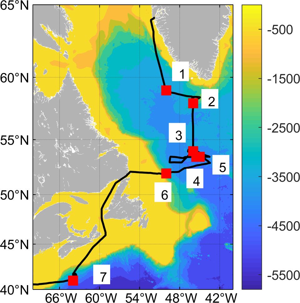
Figure 1. Observation stations and cruise trajectory (the colorbar represents the depth in meters).

For the first 20 days, the vessel operated in the Labrador Sea, south of Greenland. From November 4 to 6, 2013, it traversed the Gulf of St. Lawrence. The final station was located south of Nova Scotia, where the ship encountered warmer waters influenced by the Gulf Stream, featuring a sea surface temperature of 20 degrees Celsius and a salinity of 36 psu. Throughout the cruise, wind speeds exceeded 15 m/s approximately 25% of the time, totaling 189 hours, with 48 hours recorded at speeds exceeding 20 m/s (Table 1). Detailed methods for acquiring and analyzing whitecap coverage data are outlined in Brumer et al. (2017).

Table 1

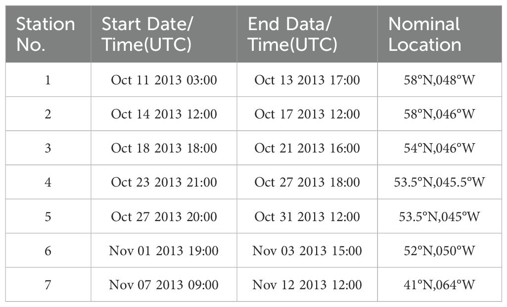
Table 1. Observation station information.

During the HiWinGS cruise, over 500 twenty-minute video segments were recorded, including 50 segments captured during the St. Jude’s Day storm. The imaging system utilized consisted of two obliquely angled Imperx Lynx 1M48 digital video cameras, each equipped with a sensing array of 1000 × 1000 elements, with a pixel size of 7.4 μm. One camera was oriented toward the starboard side, while the other was mounted on the port side, facilitating accommodation of varying lighting conditions. Wide field-of-view (FOV) lenses, with a 68.78°FOV and a 6-mm focal length, were employed. The cameras operated at a frame rate of 20 Hz throughout the HiWinGS cruise. Initial visual quality control procedures resulted in the exclusion of video segments affected by sun glare or suboptimal lighting conditions. Additionally, segments containing birds, which were prone to being misidentified as whitecaps, were also discarded. Whitecaps were subsequently isolated in the preprocessed and rectified images using the automated whitecap extraction (AWE) algorithm (Callaghan and White, 2009). For detailed procedures, refer to Brumer et al. (2017).

3 Results

3.1 Characteristics of wind and waves at different stations

Figures 2, 3 illustrate the characteristics of wind(observed wind speed at measurement height), wind waves, and swell at different stations. Station 1 was predominantly influenced by strong northerly winds. Wind speeds stayed above 15 m/s for around 12 hours before decreasing on October 13. The wind waves aligned with the wind direction, while the swell direction shifted from southwest to align with the wind waves. Starting from October 13, while the significant wave height (SWH) of wind waves decreased, the swell increased, reaching a maximum of nearly 6 meters. Station 2 experienced very strong northeastern winds with substantial wind waves. Wind speeds exceeded 20 m/s for approximately 16 hours on October 14-15. The swell direction at Station 2 was relatively chaotic, and its height remained below 2 meters, thus wind waves were the predominant feature. Station 3 was characterized by a gradual and steady increase in northeastern wind over October 19, accompanied by the development of wind waves. The wind speed peaked at about midnight on October 20, with approximately 9 hours of wind speeds exceeding 15 m/s, followed by a gradual reduction in wind and wave conditions into October 21. The swell direction was generally consistent with the wind wave direction. As the wind speed increased, both wind waves and swell showed an increasing trend. The swell was not directly influenced by changes in wind speed, and after October 21, the swell exceeded the height of the wind waves.

Figure 2

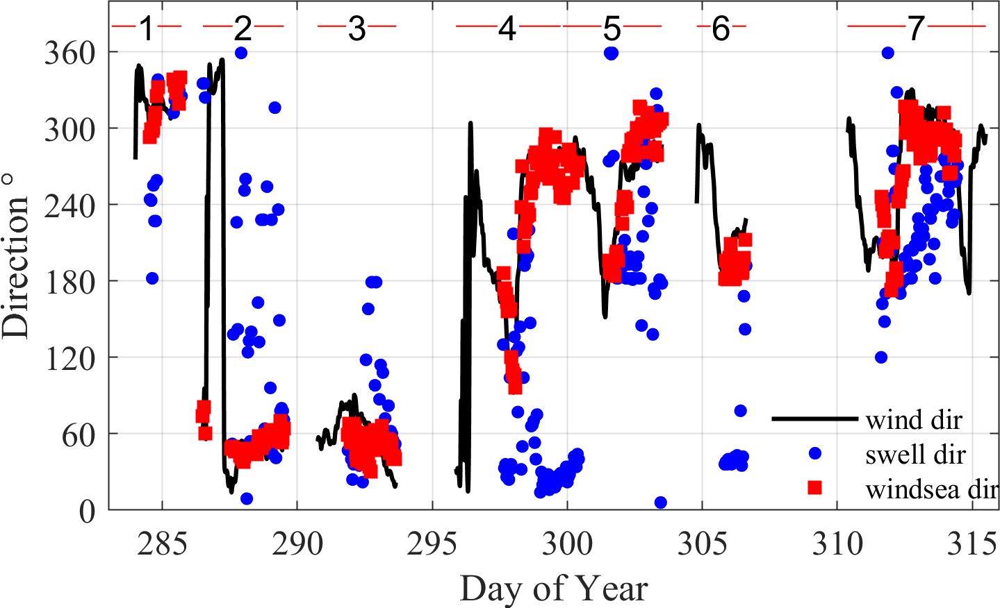
Figure 2. The directions of wind, wind waves and swell at different stations (The numbered line segments represent the time span covered at different stations.).

Figure 3

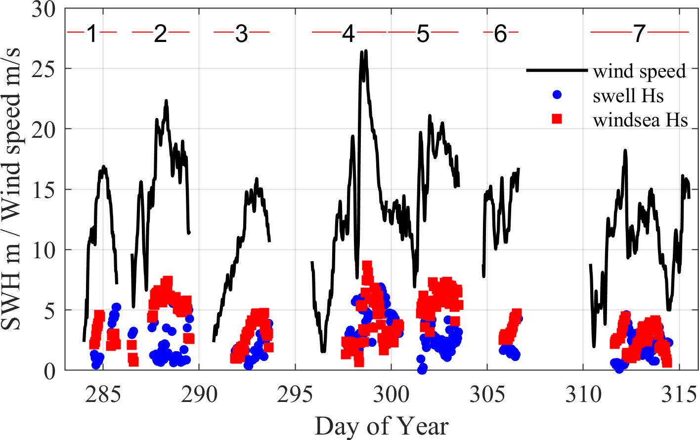
Figure 3. The SWH of wind waves and swell and wind speed at different stations (The numbered line segments represent the time span covered at different stations.).

Starting at 1200 on October 23, as a low-pressure system approached, the wind direction shifted from southerly to easterly, with speeds gradually increasing to 20 m/s at Station 4. Following the passage of the low-pressure eye, wind speeds dropped to approximately 6 m/s. Subsequently, from 0700 to 0800 on October 25, westerly winds rapidly increased to over 25 m/s, leading to the development of a full wind waves approximately 10 meters under the influence of westerly winds. Wind speeds dropped below 20 m/s shortly after midnight on October 26 and continued to decline throughout the day, although wave heights remained large. As shown in Figure 3, the swell dominated during this period at Station 4, reaching a maximum of 7 meters. The nearly 200° difference between the directions of wind waves and swell led to a chaotic sea state.

Station 5 also exhibited chaotic and mixed sea states, with strong swell from the northeast (originating from the northern lobe of the October 25 low-pressure system) combined with wind waves from strong westerly winds. The direction difference between swell and wind waves was around 120°, with swell reaching a maximum of 4 meters. Station 6, located just near the continental shelf, experienced relatively calm sea conditions. The swell was relatively stable, with wind waves reached a maximum of around 5 meters. The final station, situated just off the continental shelf, initially had calm sea conditions. Strong southerly winds developed on November 7. By 0600 on November 8, a cold front passed, and winds rapidly diminished and veered to the north. Another cold front passed during November 10-11, causing wind speeds to grow to approximately 15 m/s and then gradually decline. Consequently, the swell direction at Station 7 was unstable, varying between 2 and 4 meters, while the wind waves exhibited fluctuations in response to wind speed changes.

The above analysis clearly demonstrates that not only do wind speeds consistently remain at a high level of 15 m/s across different stations, but the mixed wave fields at each station also exhibit significant differences. These differences are mainly determined by the states of wind waves and swell. Among the stations, Station 4 and Station 5 experienced the most chaotic sea conditions, followed by Station 6 and Station 2. Stations 1, 3, and 7 were primarily dominated by wind waves.

3.2 Validation of whitecap statistical physical models

Figure 4 presents a comparison between the whitecap coverage theoretical model results and observational data across different sites, aiming to evaluate the adaptability of WSPM under high sea state conditions and explore potential areas for improvement. Initially, missing values and outliers in the observational data for each site were addressed to ensure the accuracy and completeness of the analysis.

Figure 4

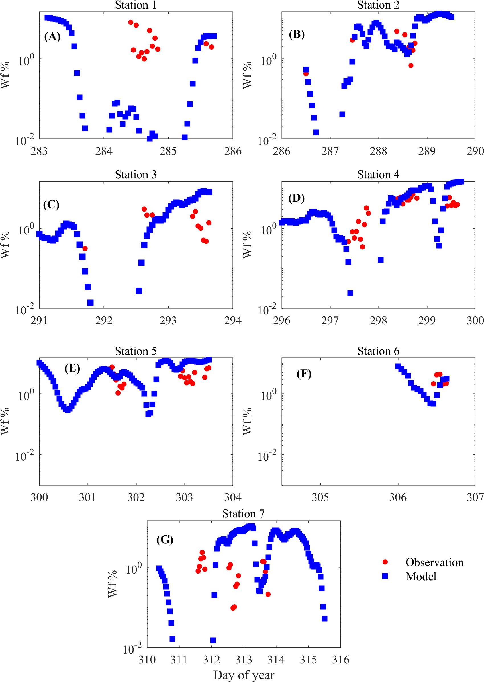
Figure 4. Model results VS observed whitecap coverage in different stations. (A-G) Different stations.

Figure 4 illustrates that the whitecap coverage characteristics vary at each site, closely corresponding to the changes in wind and wave conditions at these locations. The theoretical model results for whitecap coverage results show very good consistency with observational data at Sites 2, 4, 5, and 6 (Figures 4B, D–F). Although discrepancies between the model results and observations are slightly larger at Site 3 (Figure 4C) compared to the aforementioned sites, the overall trends of the theoretical model results closely align with the observational data. However, the theoretical model exhibits some limitations in capturing the observational data accurately, particularly at Sites 1 and 7(Figures 4A, G), where the discrepancies are more pronounced.

The theoretical results are primarily based on wave parameters from ECMWF Reanalysis 5th Generation (ERA5). To further investigate the causes of these discrepancies at Sites 1 and 7, we compared the reanalysis dataset used for calculating whitecap coverage with the observational data to identify potential differences. Figures 5, 6 provide comparisons of the SWH and mean wave period (MWP) from ERA5 with observational data for Sites 1 and 7, respectively. These figures show that the SWH and MWP from ERA5 are generally consistent with the observational data, with some exceptions where discrepancies are larger (e.g., at Station 7 at 312.5 days). Additionally, the error between ERA5 and observational data at Station 1 is noticeably larger than at Station 7, which may be one of the reasons for the discrepancies between the theoretical model results and the observations.

Figure 5

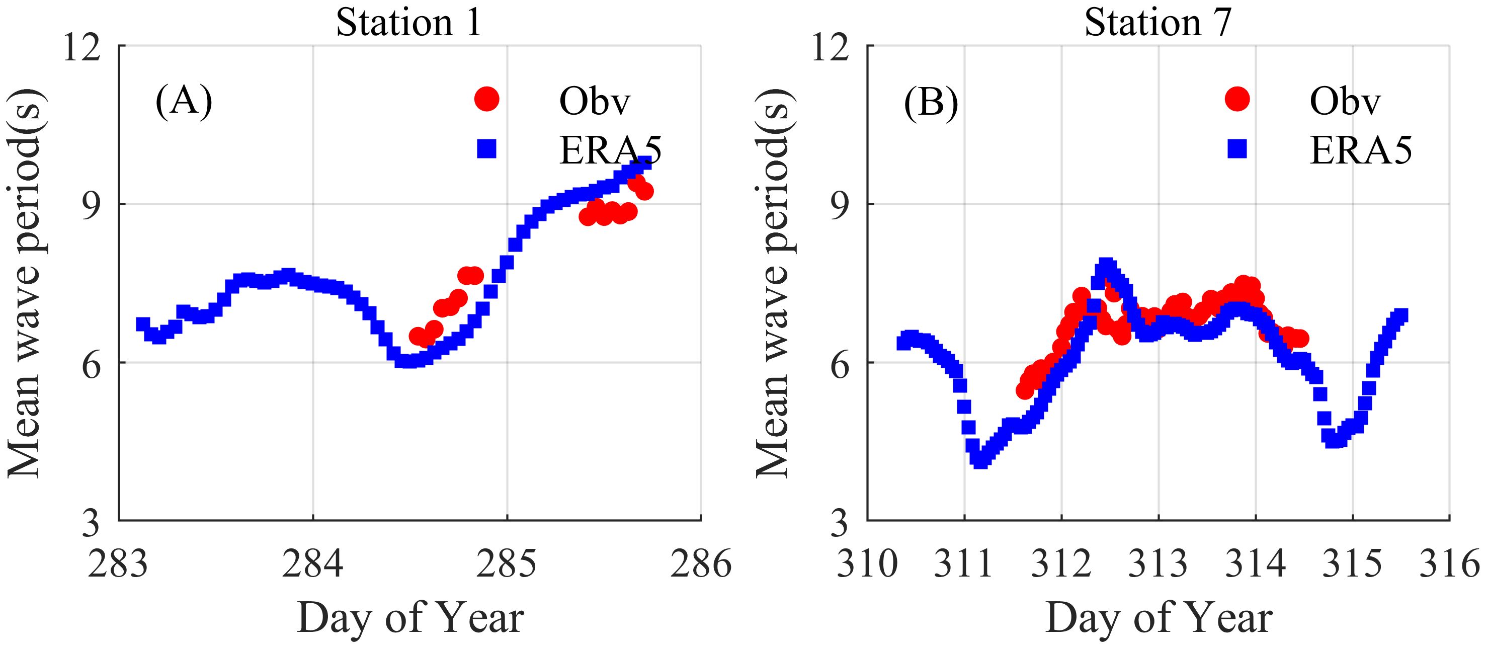
Figure 5. Comparison of significant wave heights from observations and ERA5 datasets at Station 1 and 7. (A) Station 1, (B) Station 7.

Figure 6

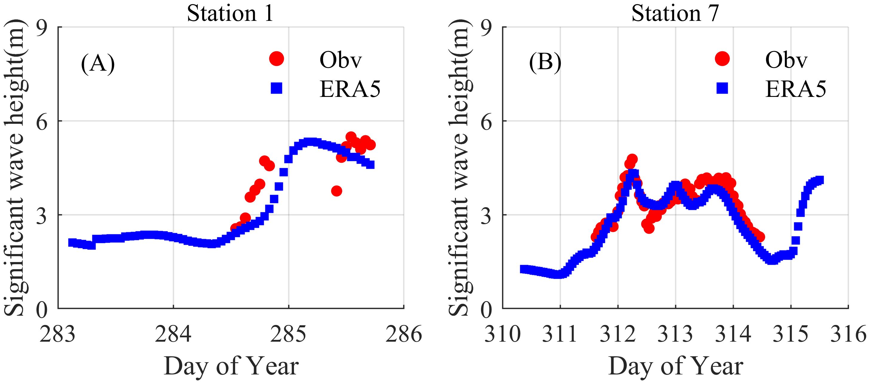
Figure 6. Comparison of MWP from observations and ERA5 datasets at Station 1 and 7. (A) Station 1, (B) Station 7.

Additionally, Sites 1 and 7 exhibit significant common characteristics in terms of wind and wave variability, with rapid fluctuations in wind speed and direction leading to unstable sea conditions. These two sites experience alternating dominance between wind waves and swell waves, with a notable increase in swell wave height following the attenuation of wind waves. Moreover, they differ from other sites in terms of the instability and degree of variability in sea conditions. Compared to Sites 2 and 3, where the wind and wave conditions are more stable, or Site 4, where swell and wind waves are more prominent, Sites 1 and 7 display a more chaotic and fluctuating interaction between wind waves and swell waves, driven by the sharp changes in wind conditions. This may also be one of the factors contributing to the larger errors observed at Sites 1 and 7.

Recognizing the unique characteristics of each observational site, including notable variations in mixed wave fields, this study compared typical wind-speed-dependent parameterization schemes against observational data. As shown in Figure 7, wind-speed-dependent parameterization schemes can effectively predict the overall trend of whitecap coverage changes with wind speed, with better performance at high wind speeds compared to low wind speeds. However, these schemes are less effective in capturing detailed variations compared to physics-based whitecap statistical models. The analysis indicates that while the trend in whitecap coverage is predominantly driven by changes in wind speed, especially under high sea states, specific information about the mixed wave fields and their interactions also significantly influences the calculation of whitecap coverage.

Figure 7

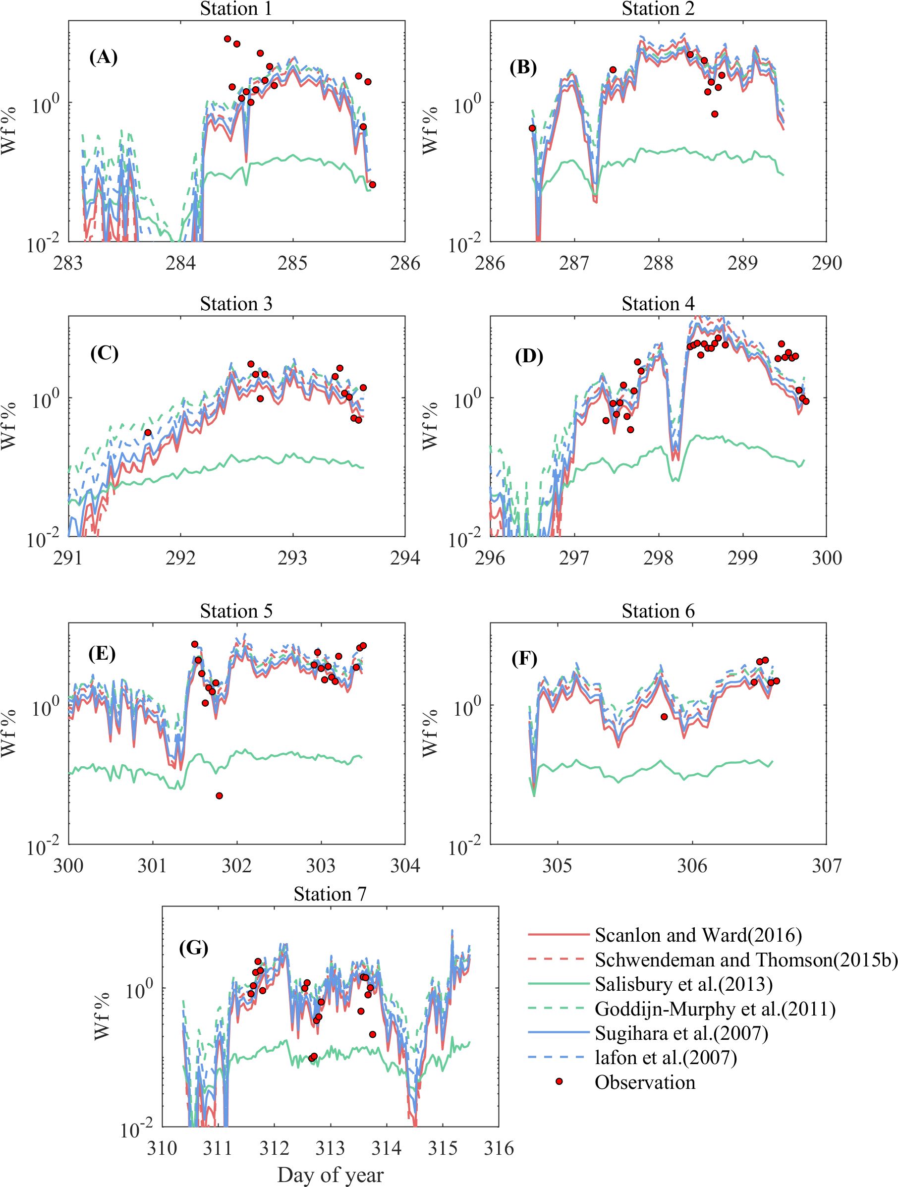
Figure 7. Scatterplots of the whitecap coverage W estimated from the wind-dependent parameterizations and observation in different stations. (A-G) Different stations.

4 Discussion and conclusions

The adaptability of the WSPM under high sea states was systematically evaluated using data from the High Wind Speed Gas Exchange Study (HiWinGS). The study demonstrated the model’s ability to capture the dynamics of whitecap coverage across various sites characterized by high wind speeds and complex mixed wave fields. The results generally showed a good agreement between the model’s predictions and the observational data, highlighting its robustness under varying oceanographic conditions. This marks the first systematic validation of the model under extreme sea states based on in-situ observational data from the HiWinGS, providing valuable insights into its practical applicability for understanding whitecap coverage in real-world scenarios.

In addition to evaluating the model’s robustness, the study addresses critical gaps in understanding whitecap dynamics. The primary cause of discrepancies may be related to the interactions between wind waves and swell at different sites. Sites 1 and 7 experienced rapid fluctuations in wind speed and direction, leading to unstable sea conditions. These sites exhibited complex mixed wave fields, with alternating dominance between wind waves and swell, along with significant changes in wave height. This variability is likely a key factor contributing to the larger errors observed at these sites. In contrast, sites 2, 3, and 4 showed more stable wind and wave conditions, with clearer relationships between wind waves and swell, resulting in better model performance.

Additionally, the use of ERA5 data for wave parameters introduces some limitations due to discrepancies between the reanalysis dataset and the observational data. The SWH and mean period from ERA5 generally align with observational data, except at certain instances, particularly at site 1, where discrepancies are more pronounced. This may partly explain the larger differences between the theoretical model results and the observations. Therefore, to improve the accuracy of the WSPM, future studies should focus on higher-frequency wave and wind data, particularly under extreme wind conditions.

The study also examines wind-speed-dependent parameterization schemes, which effectively capture the general trend of whitecap coverage with wind speed, especially at high wind speeds. However, these schemes are less effective in capturing the detailed variations in wave and wind interactions compared to physics-based whitecap statistical models. While wind-speed-dependent schemes predict the overall trend, they fall short in reflecting the complexities of the wave field in high sea states.

In conclusion, the WSPM demonstrates considerable adaptability and reliability in predicting whitecap coverage under high sea states. This study makes three significant contributions: (1) it provides the first systematic validation of the model under extreme sea conditions; (2) it identifies and quantifies the limitations of reanalysis data in capturing wave processes; (3) it advances the understanding of the influence of mixed wave fields on whitecap dynamics. These contributions underscore the importance of integrating high-resolution wave data into future models to enhance their accuracy. This work fills a major gap in the current understanding of whitecap dynamics and provides a foundation for future model improvements and more accurate predictions in complex ocean environments.

Future research should focus on refining the input data, particularly wave parameters, and exploring additional factors such as atmospheric stability and sea surface temperature. This will help improve the model’s accuracy and expand its applicability to a broader range of oceanographic conditions, ultimately contributing to a deeper understanding of critical processes at the air-sea interface.

Data availability statement

The original contributions presented in the study are included in the article/supplementary material. Further inquiries can be directed to the corresponding author/s.

Author contributions

YS: Conceptualization, Data curation, Formal Analysis, Investigation, Methodology, Software, Validation, Writing – original draft, Writing – review & editing. YY: Conceptualization, Funding acquisition, Project administration, Supervision, Writing – original draft, Writing – review & editing. JQ: Data curation, Resources, Software, Writing – review & editing. HW: Data curation, Methodology, Software, Writing – review & editing.

Funding

The author(s) declare that financial support was received for the research, authorship, and/or publication of this article. This work was supported by the National Key Research and Development Program of China with grant number 2021YFC3101604.

Acknowledgments

We appreciate the reviewers for their comments and suggestions, which helped to improve the quality of this manuscript. We are deeply grateful to the High Wind Speed Gas Exchange Study (HiWinGS) team for making their observational data available, which was instrumental in validating our model and advancing our understanding of whitecap dynamics under high sea state conditions.

Conflict of interest

The authors declare that the research was conducted in the absence of any commercial or financial relationships that could be construed as a potential conflict of interest.

Publisher’s note

All claims expressed in this article are solely those of the authors and do not necessarily represent those of their affiliated organizations, or those of the publisher, the editors and the reviewers. Any product that may be evaluated in this article, or claim that may be made by its manufacturer, is not guaranteed or endorsed by the publisher.

References

Anguelova M. D., Webster F. (2006). Whitecap coverage from satellite measurements: A first step toward modeling the variability of oceanic whitecaps. J. Geophys. Res. 111, C03017. doi: 10.1029/2005JC003158

Crossref Full Text | Google Scholar

Asher W., Wanninkhof R. (1998). The effects of bubble-mediated gas transfer on purposeful dual-gaseous tracer experiment. J. Geophys. Res. 103, 10555–10560. doi: 10.1029/98jc00245

Crossref Full Text | Google Scholar

Banner M. L., Peregrine D. H. (1993). Wave breaking in deep water. Annu. Rev. Fluid Mech. 25, 373–395. doi: 10.1146/annurev.fl.25.010193.002105

Crossref Full Text | Google Scholar

Brumer S. E., Zappa C. J., Brooks I. M., Tamura H., Brown S. M., Blomquist B. W., et al. (2017). Whitecap coverage dependence on wind and wave statistics as observed during SO GasEx and HiWinGS. J. Phys. oceanography 47, 2211–2235. doi: 10.1175/JPO-D-17-0005.1

Crossref Full Text | Google Scholar

Callaghan A. H., White M. (2009). Automated processing of sea surface images for the determination of whitecap coverage. J. Atmos. Oceanic Technol. 26, 383–394. doi: 10.1175/2008JTECHO634.1

Crossref Full Text | Google Scholar

Donelan M. A. (1990). “Air–sea interaction,” in The Sea, vol. 9 . Eds. Mehaute B. L., Hanes D. M. (USA: Ocean EngineeringScience, Wiley-Interscience), 239–292.

Google Scholar

ECMWF (2020). ECMWF Fact Sheet (Bracknell UK: European Centre for Medium-Range Weather Forecasts. Technical Report).

Google Scholar

Frew N. M. (1997). “The role of organic films in air-sea gas exchange,” in The Sea Surface and Global Change. Eds. Liss P. S., Duce R. A. (Cambridge, United Kingdom: Cambridge University Press), 121–172.

Google Scholar

Jones I. S. F., Toba Y. (2001). Wind Stress over the Ocean (Cambridge, United Kingdom: Cambridge University Press).

Google Scholar

Kanamitsu M., Ebisuzaki W., Woollen J., Yang S. K., Hnilo J. J., Fiorino M., et al. (2002). NCEP–DOE AMIP-II reanalysis (R-2). Bull. Am. Meteorological Soc. 83, 1631–1643. doi: 10.1175/bams-83-11-1631

Crossref Full Text | Google Scholar

Lamarre E., Melville W. K. (1991). Air entrainment and dissipation in breaking waves. Nature 351, 469–472. doi: 10.1038/35003952

Crossref Full Text | Google Scholar

Melville W. K. (1996). The role of surface-wave breaking in air-sea interaction. Annu. Rev. Fluid Mech. 28, 279–321. doi: 10.1146/annurev.fl.28.010196.001431

Crossref Full Text | Google Scholar

Monahan E. C., Spillane M. C. (1984). “The role of oceanic whitecaps in air-sea gas exchange,” in Gas Transfer at Water Surfaces. Eds. Brutsaert W., Jirka G. H. (Netherlands: D. Reidel), 495–503.

Google Scholar

Moore K. D., Voss K. J., Gordon H. R. (2000). Spectral reflectance of whitecaps: Their contribution to water-leaving radiance. J. Geophys. Res. 105, 6493–6499. doi: 10.1029/1999JC900334

Crossref Full Text | Google Scholar

Myrhaug D., Holmedal L. E. (2008). Effects of wave age and air stability on whitecap coverage. Coast. Eng. 55, 959–966. doi: 10.1016/j.coastaleng.2008.03.005

Crossref Full Text | Google Scholar

Saha S., Moorthi S., Pan H. L., Wu X., Wang J., Nadiga S., et al. (2010). he NCEP climate forecast system reanalysis. Bull. Am. Meteorological Soc. 91, 1015–1057. doi: 10.1175/2010BAMS3001.1

Crossref Full Text | Google Scholar

Spillane M., Monahan E. C., Bowyer P., Doyle D., Stabeno P. J. (1986). “Whitecaps and global fluxes,” in Oceanic Whitecaps (Germany: Springer), 209–218.

Google Scholar

Stramska M., Petelski T. (2003). Observations of oceanic whitecaps in the north polar waters of the Atlantic. J.Geophys. Res. 4504, 1121–1142. doi: 10.1029/2002jc001321

Crossref Full Text | Google Scholar

Wang H., Yang Y., Sun B., Shi Y. (2017). Improvements to the statistical theoretical model for wave breaking based on the ratio of breaking wave kinetic and potential energy. Sci. China Earth Sci. 59, 1–8. doi: 10.1007/s11430-016-0053-3

Crossref Full Text | Google Scholar

Woolf D. K. (1997). “Bubbles and their role in air–sea gas exchange,” in The Sea Surface and Global Change. Eds. Liss P. S., Duce R. (United Kingdom: Cambridge University Press), 173–206.

Google Scholar

Woolf D. K., Leifer I. S., Nightingale P. D., Rhee T. S., Bowyer P., Caulliez G., et al. (2007). Modelling of bubble-mediated gas transfer: Fundamental principles and a laboratory test. J. Mar.Syst. 66, 71–91. doi: 10.1016/j.jmarsys.2006.02.011

Crossref Full Text | Google Scholar

Yuan Y., Han L., Hua F., Zhang S., Qiao F., Yang Y., et al. (2009). The statistical theory of breaking entrainment depth and surface whitecap coverage of real sea waves. J. Phys. Oceanogr. 39, 143–161. doi: 10.1175/2008JPO3944.1

Crossref Full Text | Google Scholar

Yuan Y. L., Hua F., Pan Z. D., Huang N. E., Tung C. (1990). Wave breaking statistics and its application in upper ocean dynamics. Sci. China Ser.B 10, 1084–1091. doi: 10.1360/yb1990-33-1-98

Crossref Full Text | Google Scholar

Zhao D. L. (2012). Progress in sea spay and its effects on air-sea interaction. Adv. Earth Sci. 27, 624–632. doi: 10.1007/s11783-011-0280-z

Crossref Full Text | Google Scholar