Effect of delayed sea ice retreat on zooplankton communities in the Pacific Arctic Ocean: a generalized dissimilarity modeling approach

Introduction: Sea ice extent increased in the Pacific Arctic Ocean during 2021 owing to the reversal of the Beaufort Gyre, unlike in previous years. The increased sea ice concentration may restore the marine ecosystem to its previous state; nevertheless, the precise conditions and mechanisms involved remain unclear.

Methods: In this study, the 2008–2017 period was defined as “the sea ice retreat year,” and its zooplankton community distribution representative was estimated using generalized dissimilarity modeling (GDM). Subsequently, we assessed the effect of delayed sea ice melt on the zooplankton community by comparing the zooplankton community of the sea ice retreat year with that in 2021.

Results: In GDM, numerous satellite parameters significantly affected the zooplankton distribution, with the highest effect during the open-water period and annual primary production (APP) and the lowest in water temperature. The effect of APP and temperature on zooplankton similarity was high around the Bering Strait owing to the advection of Pacific copepods (Eucalanus bungii, Metridia pacifica, and Neocalanus spp.) and synchronized inflow of warm Pacific water. Under significant warming scenarios (Shared Socioeconomic Pathway [SSP]1-2.6 and SSP5-8.5), GDM-based multiple effects predicted that the zooplankton communities in high latitudes will be more affected than those on the southern shelf (northern Bering Sea to southern Chukchi Sea). In 2021, the total abundance across the northern Bering Sea to the Chukchi Sea shelf region was lower than that of the community during the sea ice retreat year. However, certain species (Limacina helicina and Pacific copepods) increased locally (northern Bering Sea and Barrow Canyon) because of the increasing volume of Pacific origin water.

Discussion: Contrary to the reported increase trend on zooplankton, low primary productivity and phenological mismatch for zooplankton may prevail in the Pacific Arctic Ocean, resulting in a low abundance during autumn 2021.

1 Introduction

In recent years, the Arctic Ocean has warmed at a rate thrice the global average, resulting in a rapid reduction in sea ice coverage during summer (Duarte et al., 2012). This sea ice retreat has explicitly been significant in the Pacific Arctic Ocean, as indicated through satellite observations (Markus et al., 2009). This results from high winter temperatures that inhibit sea ice growth and south winds in the Beaufort Sea, pushing the sea ice northward (Comiso et al., 2008), and a feedback effect where reduced sea ice contact with the Alaskan coast accelerates the sea ice circulation (Shimada et al., 2006). Along the Alaskan coast, the inflow of warm Pacific water from the Bering Sea is the most crucial factor for sea ice retreat (Shimada et al., 2006). This water transports a significant amount of oceanic heat to the Pacific Arctic Ocean (Woodgate et al., 2010), and its inflow increased in volume from 2001–2014 (Woodgate, 2018).

The inflow of Pacific water affects both marine environmental conditions and ecosystems. Anadyr water that originates from the Anadyr Bay is cold and nutrient-rich. It consistently supports high primary production in the northern Bering Sea and southern Chukchi Sea (Springer and McRoy, 1993; Cota et al., 1996). Additionally, this water and Bering shelf water transports Pacific copepods to the Arctic Ocean (Matsuno et al., 2011; Ershova et al., 2015; Pinchuk and Eisner, 2017). In contrast, Alaska Coastal Water, flowing northward along the Alaskan coast, is warm with low nutrient levels, inhabiting coastal zooplankton and hydrozoa (Pinchuk and Eisner, 2017). The inflow of these Pacific waters varies seasonally, peaking during summer (Woodgate, 2018). In response to these seasonal variations, the zooplankton communities undergo monthly alterations (Kimura et al., 2020).

Key responses in zooplankton are shifts in phenology, body size, geographical range, and contribution to the biological carbon pump toward warming (Ratnarajah et al., 2023). In the Pacific Arctic Ocean, numerous studies have been conducted on the relationship between sea ice alteration and the community structure of zooplankton. For example as phenological changes, in the northern Bering Sea, the sea ice melt season began a month earlier than usual in 2018, which delayed the spring phytoplankton bloom and resulted in chlorophyll a concentrations ten times lower than usual (Huntington et al., 2020). Additionally, this has been reflected in the secondary producers (zooplankton), with reports of delayed reproductive timing in large copepods (Kimura et al., 2022). As size changes, it has been indicated that the reduction in zooplankton size class during summer reduces energy transfer efficiency to higher trophic levels (Kumagai et al., 2023). Regarding geographical range in zooplankton, time-series data analysis of the zooplankton communities in the Chukchi Sea during the 1946–2012 period revealed an increasing abundance of Pacific copepod Neocalanus spp. and Arctic copepod Calanus glacialis (Ershova et al., 2015). Abe et al. (2020) assessed temporal alterations in the horizontal distribution of zooplankton communities in the Pacific Arctic Ocean using samples from 2008–2017. As significant environmental drivers to the abundance of C. glacialis, positive effects by the open period of sea ice and integrated mean salinity (IMS), and a negative effect by annual mean temperature were revealed in the Chukchi Shelf using generalized linear modeling. Therefore, studies based on long-term datasets have only analyzed the relationship between sea ice alteration and specific species, and it remains unclear how the entire zooplankton community may alter.

To evaluate the relationship between the entire zooplankton community and sea ice alteration, a long-term data set with a strong statistical approach is required. For example, broad-scale biogeographic patterns on zooplankton communities across the entire Southern Ocean are predicted by Generalized dissimilarity modeling (GDM) using Continuous Plankton Recorder (CPR) data (Hosie et al., 2014). GDM is a statistical method used to predict the distribution of biological communities over broad spatial scales (Ferrier et al., 2007). It statistically connects biological community data from field surveys with environmental variables derived from satellite images to estimate community similarities over broad spatial scales (Ferrier et al., 2007). GDM based on freshwater fish, large invertebrates, and environmental variables has been used to classify terrestrial rivers for appropriate ecosystem management (Leathwick et al., 2010). Additionally, GDM can be used to generate predictive models of biological distributions by adjusting the environmental variables as required (Ferrier et al., 2007). Therefore, GDM is anticipated to elucidate the relationship between sea ice alterations and zooplankton communities.

The sea ice decline trend is inconsistent in the Pacific Arctic Ocean, and irregular phenomena have been observed locally in recent years (Stabeno and Bell, 2019; Moore et al., 2022). In the northern Bering Sea, no clear trend in sea-ice extent has been observed (Walsh et al., 2017), however, a remarkably low sea-ice extent in winter 2017–2018 with no cold pool is reported (Cornwall, 2019; Stabeno and Bell, 2019). In the northern Chukchi Sea and the Beaufort Sea, the Beaufort High disappeared during the winter of 2020, causing a counterclockwise reversal of the Beaufort gyre (Ballinger et al., 2021; Moore et al., 2022). This is because enhanced cyclone activity over the central Arctic collapsed the Beaufort High during winter (Ballinger et al., 2021; Moore et al., 2022). In that case, sea ice in the Beaufort Sea shifted eastward and was transported from the Chukchi Sea to the Beaufort Sea, resulting in an increase in sea ice concentrations in 2021 (Moore et al., 2022). This delayed sea ice retreat is believed to affect zooplankton with shorter life cycles; however, detailed studies on this phenomenon have not been reported in the Pacific Arctic Ocean.

In this study, the 2008–2017 period was defined as the sea ice retreat year, and its representative zooplankton community distribution was estimated using GDM. Subsequently, we assessed the effect of delayed sea ice melt by comparing the zooplankton community of the sea ice retreat year with that in 2021.

2 Materials and methods

2.1 Satellite data

Raster data for the Pacific Arctic Ocean from 2008–2021 were derived from the Advanced Microwave Scanning Radiometer 2 (AMSR-2) operated by the JAXA Earth Observation Research Center. These data include the open-water period (days), melt day, annual median temperature (AMtemp, °C), annual median chlorophyll a (AMchl, µg L^-1), and annual net primary production (APP, mg C m^-2 yr^-1). The data have a daily time frequency and a spatial resolution of 72 km because the spatial resolution can offer the highest number of field stations without lacking a part of these satellite data at the station. Based on the open water period and melt day, the 2008–2017 period and 2021 were defined as the early sea ice melt year and delayed sea ice melt year, respectively (Supplementary Figure S1). Additionally, sea ice edge data for September 22, 2021—the median date of the 2021 survey period—were obtained from the VISHOP of the Arctic Data Archive System (ADS) (https://ads.nipr.ac.jp/vision-contents).

2.2 Field samplings

Sampling was conducted at 385 stations in the Pacific Arctic Ocean bounded by 64–79°N and 174°E–133°W during August–October 2008, September–October 2010, September–October 2012, August–October 2013, September 2014, September 2015, August–September 2016, August–September 2017, and August–October 2021 (Supplementary Figure S2). Field samplings were conducted aboard either the R/V Mirai or Canadian icebreaker Amundsen. Zooplankton samples were collected by vertical towing a NORPAC net (0.45 m mouth diameter, 335 µm mesh) from a depth of 150 m (for stations deeper than 150 m) or from 7 m immediately above the seafloor (for stations shallower than 150 m) to the surface. The zooplankton samples were immediately fixed in 5% buffered formalin. The volume of water filtered through the net was calculated from the rotation number of a one-way flow meter (Rigosha Co., Ltd., Bunkyo-ku, Tokyo, Japan) attached to the center of the net mouth. At each station, vertical profiles of water temperature, salinity, and chlorophyll a (Chl. a) were measured using a Conductivity, Temperature, Depth (CTD) profiler (Sea-Bird Electronics Inc., SBE911 plus). The zooplankton abundance and in-situ hydrography data during 2008–2017 were obtained from Abe et al. (2020).

2.3 Sample analysis

Zooplankton fixed samples (n = 46) from 2021 were divided into 1/4–1/8 sub-samples using a Motoda splitter (Motoda, 1959). Zooplankton in the subsamples were identified and counted for the taxonomic level (Order–Phylum) under a dissecting microscope (SMZ-10; Nikon). Copepods were identified at the species or genus level based on Brodsky (1967). Owing to the morphological similarity between C. glacialis and Calanus marshallae (Frost, 1974), these species were not distinguished and were counted as C. glacialis/marshallae. Zooplankton abundance (ind. m^-2) was calculated using the filtered water volume (F: m^-3) calculated using the data of flowmeter, tow distance (L), split ratio (s), and the number of each species/taxon (N, ind.) using the following equation.

$$\mathit{\text{Abundance}}=\frac{\mathit{\text{N}}\times \mathit{\text{L}}}{\mathit{\text{F}}\times \mathit{\text{s}}}$$

To examine stages of Limacina helicina at their highly abundant stations, twenty L. helicina individuals were randomly selected from a sample collected north of St. Lawrence Island in 2021. Their shell sizes were measured using an eye-piece micrometer under a microscope to calculate their average size.

2.4 General zooplankton community in the sea ice retreat year based on GDM

GDM was created using the “gdm” package in R [version 4.3.2, R Core Team (2023)] to obtain the zooplankton community distribution representative of the sea ice retreat year (cf. Ferrier et al., 2007). Supplementary Figure S3 illustrates the GDM process in this study. Zooplankton abundance (ind. m^-2) for 2008-2017 was used as in-situ biological data. For the in-situ environmental data, integrated mean temperature (IMT), integrated mean salinity (IMS), integrated chlorophyll a (Ichl), sea surface temperature (SST), and sea surface chlorophyll a (Schl) were calculated. The integrated depth was the same as the net towing depth (i.e., from a depth of 150 m or from 7 m immediately above the seafloor) at each station. Satellite data (open-water period, melt day, AMtemp, AMchl, and APP) from sampling stations were extracted from the raster data (cf. 2.1). These datasets were incorporated into the GDM to select significant data from satellite observations (Supplementary Figure S3) (cf. Ferrier et al., 2007). Environmental variables were fitted by the I-spine function, and the sum of I-spline coefficients was obtained (Supplementary Figure S4). Subsequently, the satellite raster data for each year from 2008–2017 were averaged using the “abind” package in R. The average satellite data, where statistically significant relationships were observed through GDM (open-water period, AMtemp, and APP in our case), were incorporated into the model, and principal component analysis was conducted. The obtained principal components 1–3 (PC1–3) were converted to RGB values, yielding a zooplankton distribution for the average sea-ice melt years (2008–2017).

Additionally, the PC1–3 values (n = 6420) were extracted and normalized (subtracting means and dividing by standard deviation). A matrix of similarity index using Euclidean distance was created for a cluster analysis using PRIMER v7 software. Based on the resulting similarity matrix, a dendrogram was constructed using the mean linkage method (Unweighted Pair Group Method using Arithmetic mean [UPGMA]: group average method) to partition the data into numerous groups at any desired similarity level. Subsequently, the in-situ zooplankton abundance corresponding to each group from 2008–2017 was extracted. Indicator Value of Species (IndVal) (Dufrêne and Legendre, 1997) was used to identify the indicator species for each group, and a similarity percentage (SIMPER) analysis (Clarke, 1993) was used to determine the contribution of each species/taxonomic group to the similarity among groups.

2.5 Data analysis based on zooplankton samples from 2021

The zooplankton abundances from 2021 (ind. m^-2) were transformed into fourth roots, and the Bray-Curtis similarity index (Bray and Curtis, 1957) was used to calculate the sample similarities. Based on the resulting similarity matrix, a dendrogram was constructed using the mean linkage method (UPGMA) to partition the data into numerous groups at any desired similarity level. To determine whether clustering was statistically significant at the 5% level, similarity profile analysis (SIMPROF) was performed. To identify the indicator species, IndVal and SIMPER were conducted. Cluster, SIMPROF, and SIMPER analyses were conducted using the PRIMER v7 software (PRIMER-E Ltd., Albany, Auckland, New Zealand), and IndVal calculations were performed using Excel.

2.6 Assessing the effect of environmental variables on zooplankton similarity

To assess how environmental alterations affected the similarity index of zooplankton communities, datasets were created using arbitrarily varied satellite data (open-water period, AMtemp, and APP), for which statistically significant relationships were observed using the GDM. We assessed the warming scenarios in IPCC AR6 (Shared Socioeconomic Pathway [SSP]1-2.6 and SSP5-8.5) by incorporating parameter alterations based on previous studies (Bryndum-Buchholz et al., 2019; Lotze et al., 2019; Nakamura and Oka, 2019; Overland et al., 2019; Khosravi et al., 2022). Sea surface temperature will increase by 1.8 and 4.4°C in the SSP1-2.6 and SSP5-8.5 scenarios, respectively (Overland et al., 2019; Khosravi et al., 2022). Regarding the open water period, the surface temperature increased by 2°C with a 99-day extended open water period in the Chukchi Sea under the SSP1-2.6 scenario (Crawford et al., 2021). The SSP5-8.5 scenario also showed a 5.5°C increase with 270 days in open water period in the Chukchi Sea (Crawford et al., 2021). According to the model projections in the Chukchi Sea (Overland et al., 2019; Crawford et al., 2021; Khosravi et al., 2022), 1.8°C increase with 90-days extended of open water period in SSP 1-2.6 and 4.4°C increase with 150-days extended of open water period (due to minimum open water period in the Chukchi Sea was 120 days) in SSP 5-8.5 were set as a condition until 2100. Primary production also increases by 5 and 10% until 2100 in the SSP1-2.6 and SSP5-8.5 scenario, respectively (Bryndum-Buchholz et al., 2019; Lotze et al., 2019; Nakamura and Oka, 2019). Following the alternated conditions, the spatial changes in the zooplankton similarity index were assumed using the “predict” function in R (Supplementary Figure S3). The similarity index is an absolute value. A low value means no change in the zooplankton community in the simulated condition (e.g., 1.8 °C increase). However, the high zooplankton similarity index suggests that the group where the high value is showing could be changed to a different neighboring group.

3 Results

3.1 Hydrography

The open-water period in 2008–2017 ranged from 150–240 days in the southern Chukchi Sea and was shorter at higher latitudes (Figure 1). A similar trend was observed in 2021, although the Chukchi Plateau and Canada Basin demonstrated a shorter open-water period than that in 2008–2017. Melt days ranged from 120–270 days during 2008–2017, with later melt days occurring at higher latitudes (Figure 1). Melt days for 2021 were similar to those of 2008–2017 in the southern Chukchi Sea but significantly later from the northern Chukchi Sea to the Chukchi Plateau. AMtemp was similar between 2008–2017 and 2021, with higher values observed in bays along the coast of Alaska. The AMchl concentration in the Bering Strait ranged from 2–3 µg L^-1 during 2008–2017, but was slightly lower at 1–2 µg L^-1 in 2021 (Figure 1). Additionally, in the Chukchi Sea, it ranged from 0–2 µg L^-1 during 2008–2017, but was low at 0–1 µg L^-1 in 2021. APP in the Bering Strait during 2008–2017 was 120000–160000 mg C m^-2 yr^-1, which was not observed in 2021 (Figure 1). However, areas with 80,000–120,000 mg C m^-2 yr^-1 expanded in the northern Bering Sea and the southern Chukchi Sea. Additionally, in the Beaufort Sea, APP ranged from 0–40000 mg C m^-2 yr^-1 during 2008–2017, but the 40000–80000 mg C m^-2 yr^-1 range was partially expanded by 2021.

Figure 1

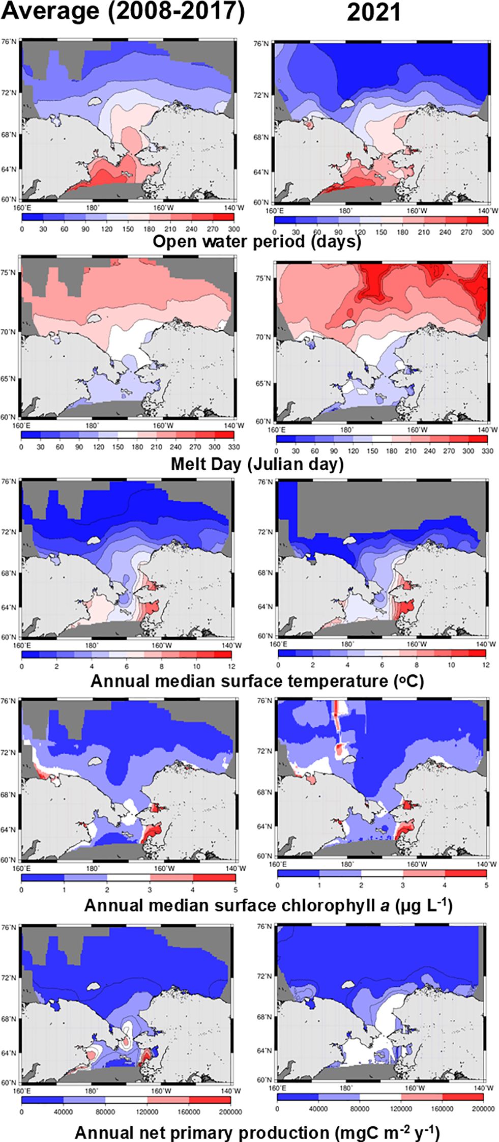
Figure 1. Average images from 2008 and 2017 (left panel) and the image from 2021 (right panel) illustrates open-water period, melt day, annual median surface temperature, annual median surface chlorophyll a, and annual net primary production, all derived from satellite observations during summers in the Pacific Arctic Ocean.

Regarding the in-situ hydrological environment data, the IMT ranged from -1.4–7.8°C, with lower and higher values in the Beaufort Sea (-1–1°C) and the Chukchi Sea (2–7.8°C), respectively (Figure 2). In 2017, numerous stations exhibited higher temperatures (6–7.8°C) than usual. The IMS ranged from 26.9–33.2, with no apparent interannual variation during 2008–2017. However, in 2021, it was low (28.9–30.0) in the Chukchi Sea and south of the Bering Strait, specifically along the coast (Figure 2). Ichl ranged from 6.9–290.4 mg m^-2 and was higher in the Chukchi Sea and lower in the Canada Basin and Beaufort Sea during 2008–2017 (Figure 2). However, in 2021, it was high in the Hanna Shoal to Canada Basin (7.8–76.7 mg m^-2) and low in the Chukchi Sea (6.8–31.4 mg m^-2). High values (105.2–175.5 mg m^-2) were observed in the Bering Strait from 2015–2017, but were lower in 2021.

Figure 2

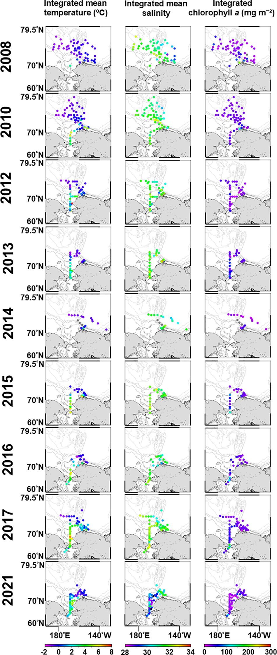
Figure 2. Interannual alterations of the in-situ hydrographic parameters from 2008–2021 during summers in the Pacific sector of the Arctic Ocean.

3.2 GDM

The GDM results identified nine significant variables: six in-situ hydrological variables (geographic distance, depth, IMT, IMS, Ichl, and Schl) and three satellite data (open-water period, AMtemp, and APP) (Supplementary Figure S4). Spline regression shapes roughly fell into three categories: those that sharply increased at low variable values (geographical distance, depth, and Schl), those that increased gradually (IMS, Ichl, and open-water period), and those that increased at high variable values (IMT, AMtemp, and APP). Specifically, the Schl (total I-spline coefficient 0.704) and IMT (total I-spline coefficient 0.505) had large maximum values, indicating their influence on the model. Additionally, the open-water period (total I-spline coefficient 0.398), AMtemp (total I-spline coefficient 0.233), and APP (total I-spline coefficient 0.193) were relatively high-influential variables.

3.3 Zooplankton communities during 2008–2017

The cluster analysis based on PC1–3 values from GDM between 2008–2017 identified eight groups in the Pacific Arctic Ocean, with a distance of 1.73. High abundances of C. glacialis/marshallae, Pseudocalanus spp., and E. bungii were identified in the southern Bering Strait, Bering Strait, and Southern Chukchi Sea groups, respectively (Figure 3; Table 1). Appendicularians and barnacles were more abundant in the Bering Strait, whereas Acartia spp. and M. pacifica were more abundant in the Southern Chukchi Sea (Table 1). The Chukchi and East Siberian Seas group occurred on the central shelf (Figure 3), with higher abundances of Pseudocalanus spp. and chaetognaths. Calanus hyperboreus, Metridia longa, Microcalanus spp., and L. helicina were the most abundant species in the Northwind Ridge group (Table 1). The area from the slope to the Beaufort Sea was occupied by the Barrow Canyon and Beaufort Sea group, which had the highest number of species. Additionally, this group had the highest mean abundance of C. glacialis/marshallae, with chaetognaths as indicator species. Canada Basin group identified in the Canada Basin had a relatively low average abundance. C. glacialis/marshallae and M. longa were abundant in this group, with hydrozoa as indicator species.

Figure 3

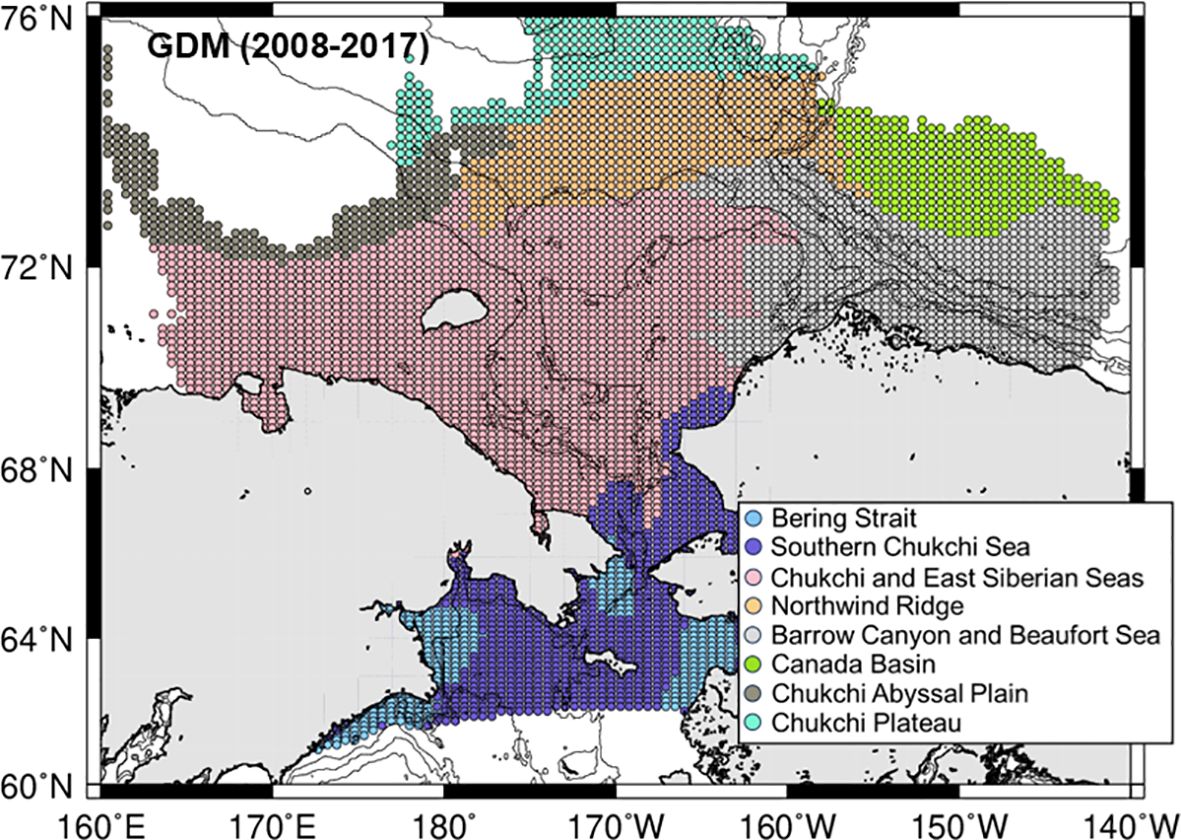
Figure 3. Horizontal distribution groups identified using a cluster analysis based on principal component (PC) values from generalized dissimilarity modeling (GDM) using the 2008–2017 data set.

Table 1

Table 1. Mean abundance of mesozooplankton in the groups identified using a cluster analysis through generalized dissimilarity modeling (GDM) using the 2008–2017 data set (cf. Figure 3) in the Pacific Arctic Ocean.

3.4 Zooplankton community in 2021

In 2021, a cluster analysis based on zooplankton abundance identified six groups (Figure 4A). These groups were named based on their distribution areas: 21_off Barrow (three stations), 21_Slope (10 stations), 21_Bering Strait (five stations), 21_Hanna Shoal (seven stations), 21_Chukchi Sea (18 stations), and 21_Coast (three stations) (Figures 4A, B). Three groups, 21_Slope, 21_Chukchi Sea, and 21_Coastal, exhibited low average abundance (< 10,000 ind m^-2) (Table 2). In the south of the Bering Strait, the 21_Bering Strait was observed, characterized by a high abundance of Pacific species, such as Metridia pacifica and E. bungii, with Pseudocalanus spp. and L. helicina being the most abundant among the six groups. In the central Chukchi Sea, two groups, 21_Chukchi Sea and 21_Coast, exhibited a low mean abundance and high abundance of C. glacialis/marshallae and chaetognath, respectively. In the 21_Hanna Shoal observed near the sea ice edge, the number of species was relatively low and the abundance of appendicularia and barnacles was significantly high (Table 2). 21_off Barrow had the highest average abundance, with C. glacialis/marshallae accounting for approximately one-third of the total abundance. Additionally, Arctic species, such as C. hyperboreus and Pacific species, including Neocalanus cristatus, Neocalanus flemingeri, and Neocalanus plumchrus, were the most abundant among the six groups. 21_Slope was identified from the slope to the Canada Basin, where Cyclopoida, M. longa, and Microcalanus spp. were abundant, with Paraeuchaeta glacialis selected as an indicator species.

Figure 4

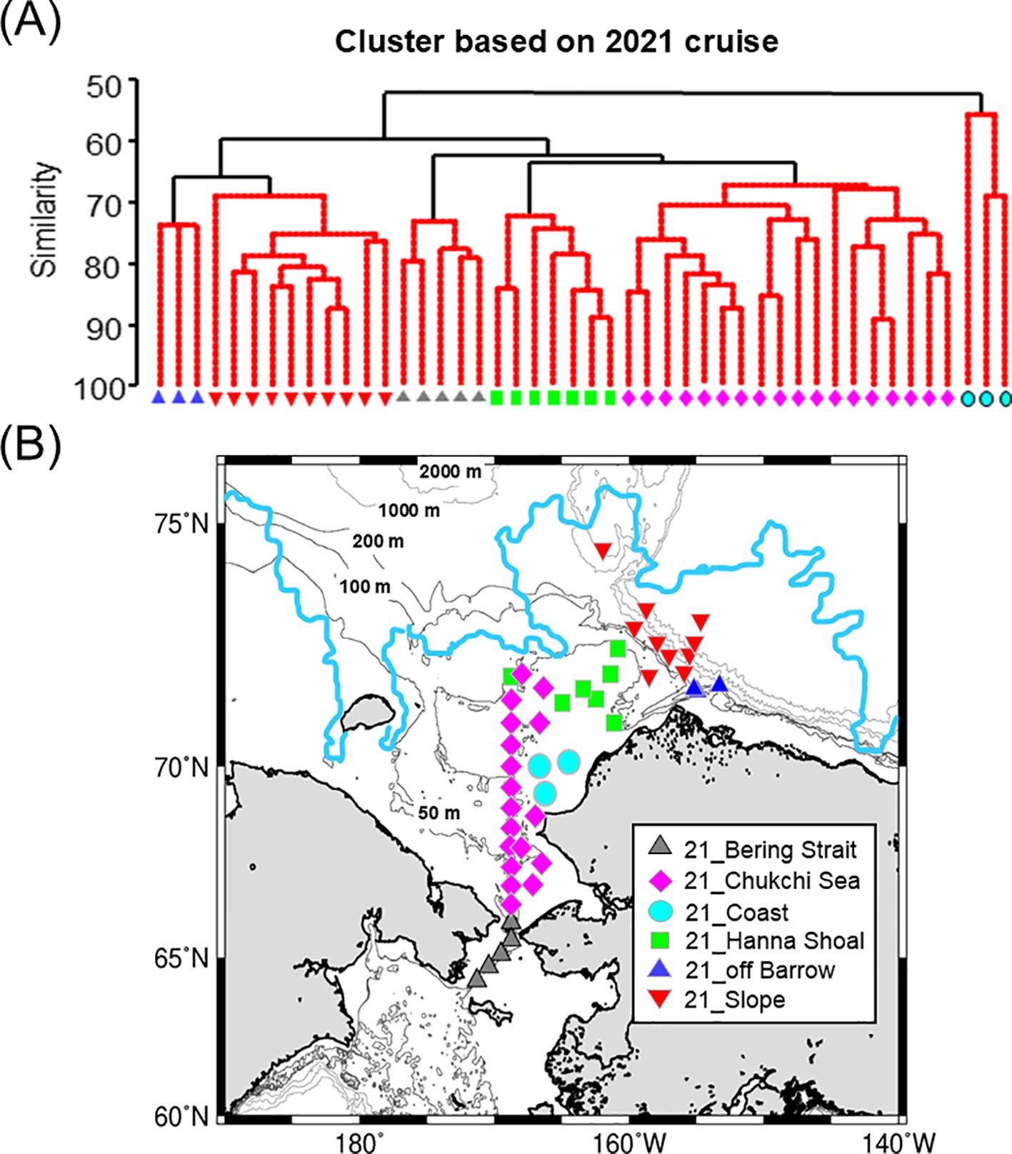
Figure 4. Results of cluster analysis based on mesozooplankton abundance in 2021 using Bray–Curtis similarity connected with Unweighted Pair Group Method using Arithmetic mean (UPGMA) (A). Six groups were identified with similarity profile (SIMPROF) test. Horizontal distribution of the groups during 2021 summer in the Pacific sector of the Arctic Ocean (B). Light blue line indicates sea ice edge at the middle September 2021. Light gray lines indicate bathymetric depth.

Table 2

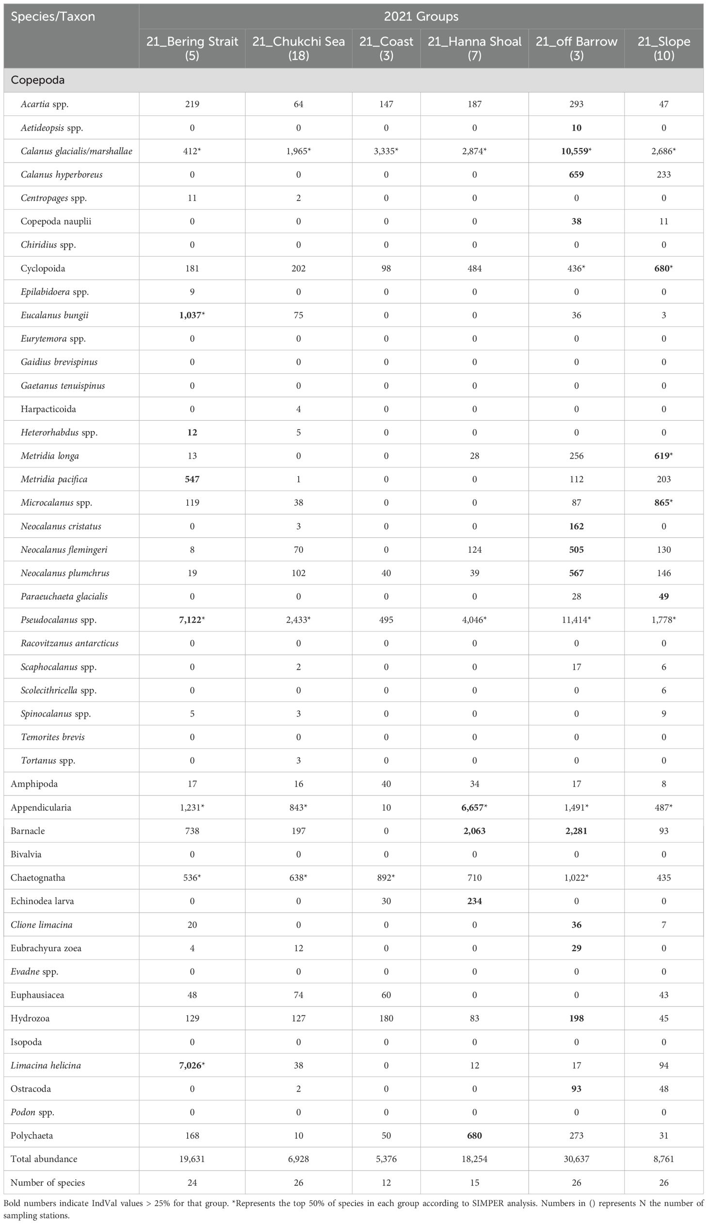
Table 2. Mean abundance of mesozooplankton in the groups identified through cluster analysis in 2021 (cf. Figure 4) in the Pacific Arctic Ocean.

3.5 Comparison of in-situ environmental conditions among communities

Comparing the 21_Bering Strait group and Bering Strait and Southern Chukchi Sea group, the IMT in 21_Bering Strait was approximately 1°C lower than that in Bering Strait and Southern Chukchi Sea group (2.25°C vs. 3.68–3.92°C) (Tables 3, 4; Figure 5). The IMS was < 30 in the 21_Bering Strait, clearly lower than that in the Bering Strait and Southern Chukchi Sea (averages of 32.39 and 31.67, respectively). Additionally, although the APP range in the 21_Bering Strait was broad (Figure 5), it was higher than that in the Bering Strait and Southern Chukchi Sea (134,028 mg C m^-2 yr^-1 vs. 69,907–115,452 mg C m^-2 yr^-1).

Table 3

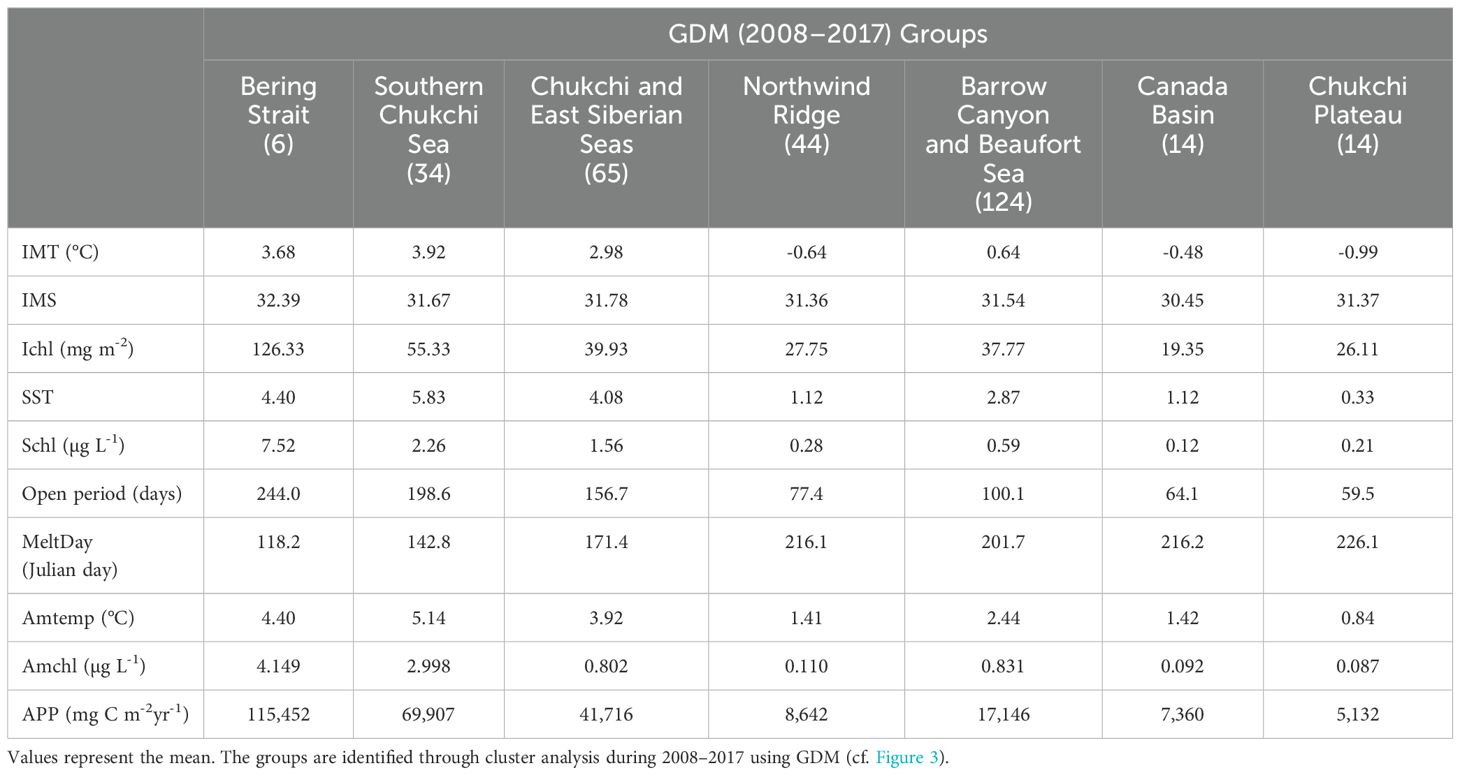
Table 3. Inter-group comparison of hydrography and satellite data during 2008–2017 in the Pacific Arctic Ocean.

Table 4

Table 4. Inter-group comparison of hydrography and satellite data in 2021 in the Pacific Arctic Ocean.

Figure 5

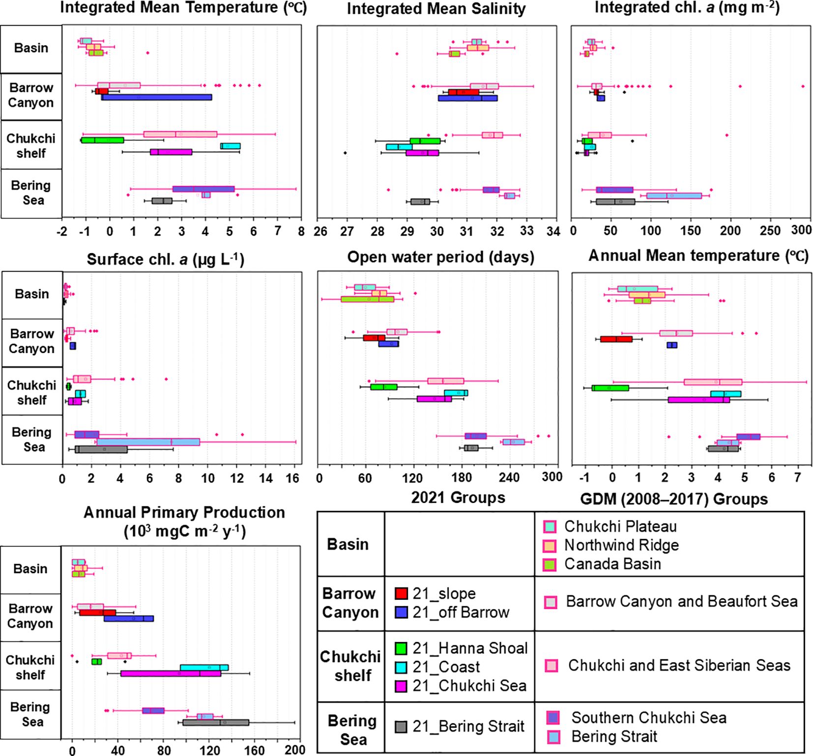
Figure 5. Inter-group comparison of hydrographic data from 2008–2021 in the Pacific Arctic Ocean. The groups are identified using cluster analysis and generalized dissimilarity modeling (GDM) (cf. Figures 3, 4).

The 21_Chukchi Sea group corresponds to the Southern Chukchi Sea and Chukchi and East Siberian Seas groups. The IMS in the 21_Chukchi Sea was lower than that in the GDM groups (29.53 vs. 31.67–31.78) (Tables 3, 4; Figure 5). Ichl was lower in 21_Chukchi Sea than that in Southern Chukchi Sea and Chukchi and East Siberian Seas (19.03 mg m^-2 vs. 39.93–55.33 mg m^-2). In contrast, the APP average in the 21_Chukchi Sea was approximately 20000 mg C m^-2 yr^-1 higher than that in the GDM groups (Tables 3, 4).

The 21_Coast group corresponds to the Chukchi and East Siberian Seas in the GDM group. IMS in the 21_Coast group was below 30 and lower than that in the GDM groups (28.73 vs. 31.78) (Tables 3, 4; Figure 5). The APP in the 21_Coast group was significantly higher than that in the Chukchi and East Siberian Seas groups (120,444 mg C m^-2 yr^-1 vs. 41,716 mg C m^-2 yr^-1).

Comparing the 21_Hanna Shoal group and Chukchi and East Siberian Seas and Barrow Canyon and Beaufort Sea groups from GDM, Schl in the 21_Hanna Shoal group was lower than that in the GDM groups (0.43 µg L^-1 vs. 0.59–1.56 µg L^-1) (Tables 3, 4; Figure 5). The average of AMtemp in 21_Hanna Shoal was below 0°C on average, lower than that in the GDM groups (-0.10°C vs. 2.44–3.92°C).

No significant differences were observed between the 21_off Barrow group and Barrow Canyon and Beaufort Sea groups in the in-situ environmental conditions (Tables 3, 4; Figure 5).

The 21_Slope group corresponds to the Northwind Ridge, Barrow Canyon and Beaufort Sea, and Canada Basin groups from GDM. AMtemp in the 21_Slope group was approximately 1°C lower than that in the GDM groups (0.21°C vs. 1.41–2.44°C) (Tables 3, 4; Figure 5). Additionally, the AMtemp in the 21_Slope was approximately 2°C lower than that in the 21_off Barrow, and the average APP was approximately 30,000 mg C m^-2 yr^-1 lower.

3.6 Predation of the zooplankton community alteration

First, the effect on the zooplankton similarity index was high in the open-water period, whereas it was relatively low in water temperature and APP based on the maximum values in each parameter (Figure 6). Spatially, the increasing open-water period (SSP1-2.6, SSP5-8.5) had a significant effect at higher latitudes near the Chukchi Plateau (sea ice edge in autumn), indicating potential alterations in the community composition of the Northwind Ridge and Chukchi Plateau. In contrast, the increasing open water period did not affect the zooplankton community in the Chukchi Sea and the East Siberian Sea. As the temperature shifted from moderately warm (SSP 1-2.6) to highly warm (SSP 5-8.5), the area of alteration in the similarity index extended northward from the northern Bering Sea to the northern Chukchi Sea (Figure 6), but the effect on the similarity index was small (0.008–0.012) comparing to the other parameters (i.e., open water period and APP). The warm conditions did not affect the zooplankton in the northern Bering Sea and Alaskan side near Bering Strait. For the APP, alterations in the similarity index were primarily observed around the Bering Strait and Anadyr Bay, and higher APP induced more effect on the similarity. In contrast, no effect on the zooplankton similarity index by APP increase was seen in the north of 70°N. In the multiple effects of the open-water period, AMtemp, and APP, SSP5-8.5 exhibited a more remarkable similarity index alteration than the SSP1-2.6 scenario. The two scenarios had similar spatial variations in the zooplankton similarity index; the highest value was in the higher latitudes near the Chukchi Plateau. The effect on zooplankton similarity gradually decreased from the higher latitude to the shelf region, and a moderate effect was seen at the Bering Strait (Figure 6).

Figure 6

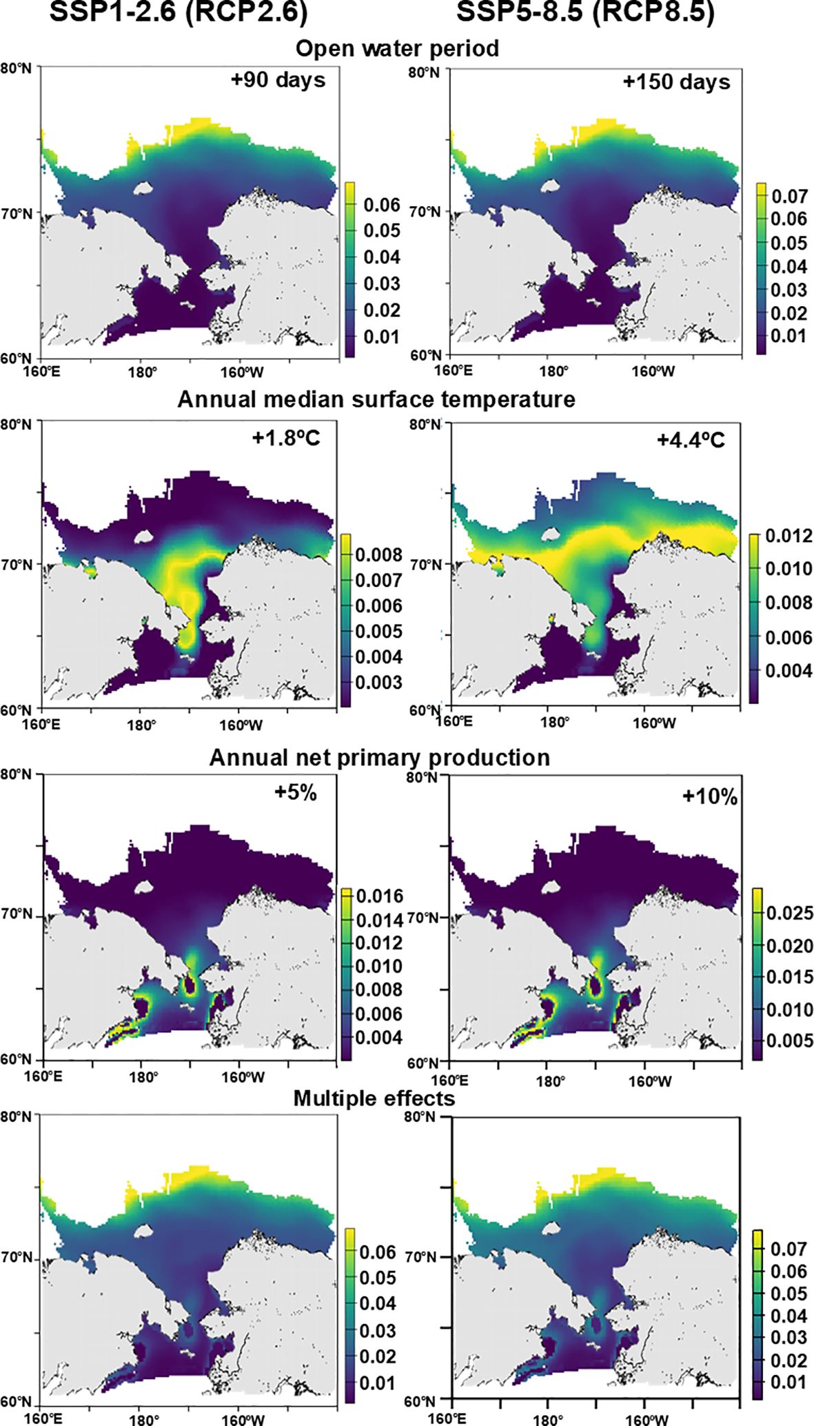
Figure 6. Spatial distribution of predicted environmental effects on the zooplankton community similarity analyzed using generalized dissimilarity modeling (GDM). The scenario is based on IPCC AR6 (SSP1-2.6 and SSP5-8.5) (Bryndum-Buchholz et al., 2019; Lotze et al., 2019; Nakamura and Oka, 2019; Overland et al., 2019; Crawford et al., 2021; Khosravi et al., 2022).

4 Discussion

4.1 Analysis of the zooplankton communities using GDM

GDM is a statistical method that connects species diversity in ecosystems with environmental variables, enabling the prediction of biological distribution over broad spatial scales (Ferrier et al., 2007). Because of its usefulness, it has been applied in the formulation of ecosystem conservation management plans (Ware et al., 2018). For example, GDM based on freshwater fish, large invertebrates, and environmental variables has been used to classify terrestrial rivers for appropriate ecosystem management (Leathwick et al., 2010). Additionally, in northwestern Australia, it is used to select suitable observation sites to monitor the distribution of terrestrial invertebrates (Ashcroft et al., 2010). An example of using GDM with marine zooplankton communities is a study that used CPR data for the entire Antarctic Ocean (Hosie et al., 2014). They predicted the general spatial distribution of the surface zooplankton community each month based on more than 25,000 in-situ biological data using GDM and cluster analysis (Hosie et al., 2014). This study used GDM to determine the representative zooplankton community distribution in the Pacific Arctic Ocean from 2008–2017 (sea-ice retreat years) and predict community alterations owing to environmental fluctuations in two scenarios. Because this method can estimate zooplankton communities over broad spatial scales by combining the biological similarity index and satellite data, GDM can directly contribute to generating insights into the conservation and management of biodiversity (Hosie et al., 2014).

Three satellite data (open-water period, AMtemp, and APP) were selected as significant parameters associated with the zooplankton community in the GDM. Regarding the open-water period and APP, the open-water period was extended by 3.5 days per decade based on satellite observations from 2003–2009 in the northern Bering and Chukchi Seas (Markus et al., 2009), consequently increasing chlorophyll a concentration (Grebmeier, 2012). In this study, the multiple effect model under significant warming scenarios (SSP1-2.6 and SSP5-8.5) indicated that ecosystem alterations were more significant at higher latitudes, whereas the effect was smaller in the previously studied regions (northern Bering Sea to southern Chukchi Sea). However, in the previously studied region, alterations in sea ice melt timing have been reported to affect phytoplankton bloom dynamics (Huntington et al., 2020; Kikuchi et al., 2020) and zooplankton reproduction and community alterations (Kimura et al., 2022). Because GDM cannot predict these seasonal or phenological alterations in plankton productivity and composition, alternative models are required. In this study, although melt day was not selected as a significant variable in GDM, its significance may be increased by considering specific seasons and regions (Huntington et al., 2020; Kimura et al., 2022).

In this study, the effect of APP alterations on zooplankton similarity was primarily observed around the Bering Strait. However, this is misaligned with the region where sea ice melting is more pronounced. Therefore, it is not because of the effect of sea ice melting but rather the susceptibility of the region to the inflow of nutrient-rich Pacific water (Springer and McRoy, 1993; Cota et al., 1996). Zooplankton similarity in the Gulf of Anadyr was also sensitively affected by the increase in APP. In the region, cyclonic circulation caused the upwelling of deeper water from the Bering basin and continued the supply of nutrients to the surface layer, resulting in intensive phytoplankton bloom (Clement et al., 2005; Iida and Saitoh, 2007). In low sea-ice production year at Anadyr polynya, which is identified as one of the most active polynyas in the Northern Hemisphere, the bottom water is occupied by Pacific-origin water, and southerly wind drive advection of the bottom water from the Bering basin region to shelf (Basyuk and Zuenko, 2020; Abe et al., 2021). Considering these oceanographic backgrounds, the affected region (i.e., Bering Strait and Gulf of Anadyr) by increased APP is reasonable. In the present study, however, since atmospheric parameters (e.g., wind direction) could not be included in GDM, the detailed impact of atmospheric forcing via sea-ice extent and water property should be investigated in the future.

A significant effect of AMtemp on zooplankton similarity was observed from the northern Bering Strait to the southern Chukchi Sea in a +1.8°C scenario. This is attributed to the inflow of warm Pacific water from the Bering Sea to the Chukchi Sea (Woodgate, 2018; Spear et al., 2019), resulting in the advection of Pacific copepods (E. bungii, M. pacifica, Neocalanus spp.) (Matsuno et al., 2011; Kim et al., 2020). On the other hand, in the +4.4°C scenario, the affected area of zooplankton similarity was predicted to be extended to the north, covering the whole shelf region, and the alternation value (approximately 0.008) in zooplankton similarity in the southern Chukchi Sea was no difference between the +1.8°C and +4.4°C scenarios. This means that the zooplankton community in the southern Chukchi Sea will reach the maximum changes by 1.8°C warmer conditions, but in the northern Chukchi Sea, East Siberian Sea, and Beaufort Sea, zooplankton community will be drastically changed by 4.4°C warmer condition.

From the above, GDM using extensive field and satellite data is a valuable method for obtaining general patterns in biological distribution. In contrast, one disadvantage of GDM is that the environmental parameters do not entirely explain the variation in biological parameters owing to limited satellite data significantly related to zooplankton. In our case, sea ice concentrations, which may affect the zooplankton community, could not be included in the GDM. Sea ice parameters (e.g., concentration, thickness, snow depth) derived by satellite observation are primary important factors in controlling solar radiation underwater (Light et al., 2008), nutrients and ice-algae dynamics (Melnikov et al., 2002), phytoplankton bloom (Ji et al., 2013). These physical and biological triggers relate zooplankton distribution and behavior (e.g., diel vertical migration) (Darnis et al., 2017), grazing activity (Campbell et al., 2009), growth and reproduction (Kimura et al., 2020, 2022). If these sea-ice parameters could be included in the GDM, the model would explain the zooplankton distribution and be able to predict the community under the sea ice. To accomplish the improvement in the model, continuous field surveys over a broad area using an icebreaker are necessary to obtain the in-situ data under sea ice.

4.2 The effect of delayed sea ice melt on the zooplankton community

Describing the interannual differences in certain species by area, the abundance of L. helicina in the Bering Strait and southern Chukchi Sea in 2021 was higher than that during 2008–2017 (7,026 vs. 0–193 ind m^-2) (Tables 1, 2) and was dominated by small individuals (data not shown). L. helicina is a hermaphrodite with developmental stages classified by shell length: veliger larvae (< 0.3 mm), juveniles (0.3–4.0 mm), male adults (4.0–5.0 mm), and female adults (> 5.0 mm) (Lalli and Wells, 1978). The majority of the L. helicina observed in 2021 averaged 0.27 mm, indicating a dominance of veliger larvae in the population of 2021. L. helicina is omnivorous, feeding on phytoplankton from spring to summer and organic particles from autumn to winter (Gannefors et al., 2005). In the Canada Basin, they spawn primarily from spring to summer, with smaller spawning events occurring in autumn (Kobayashi, 1974). In the regions around Spitsbergen Island, veliger larvae and juveniles were observed in spring, adults in July, and veliger larvae in September, indicating spawning from late summer to fall (Gannefors et al., 2005). In the 21_Bering Strait, there was minimal alteration in the melt day and Ichl compared with the community by GDM, but lower IMT and higher APP were observed (Tables 3, 4). In the northern Bering Sea, cold Anadyr water from Anadyr Bay flows in, forming cold water masses with upwelling along the Siberian coast northwest of St. Lawrence (Kawaguchi et al., 2020). It contains high levels of nutrients, resulting in high primary production and chlorophyll a concentrations (Springer and McRoy, 1993; Cota et al., 1996). In this study, the high abundance of veliger larvae resulted from the nutrient supply within the euphotic zone, provided by cold Anadyr water with high nutrients. This results in an increase in phytoplankton and triggers the reproduction of this species.

In 2021, the communities in the northern Chukchi Sea (21_Chukchi Sea group, 21_Coast group, and 21_Hanna Shoal group) were significantly reduced in total abundance because of delayed sea ice retreat. Among these, the 21_Coast group exhibited an earlier melt day, higher IMT (4.93°C), and lower IMS (28.7) than the other two communities. This region is characterized by the formation of polynyas owing to easterly winds (Hirano et al., 2016, 2022) and the inflow of warm Alaska Coastal Current along the Alaskan coastline (Pickart et al., 2023). The Alaska Coastal Current contains a high abundance of hydrozoa, which were relatively more abundant in the 21_Coast group (Table 2). The 21_Hanna Shoal group had the highest abundance of appendicularians in 2021. In 2021, this region was at the sea ice edge during the sampling period, and both the IMT and IMS were low (Table 4). Higher abundances of appendicularians, specifically Oikopleura vanhoeffeni, have been observed near the sea ice edge (Hopcroft et al., 2010). The increase in appendicularian abundance observed in this group was likely due to the dense distribution near the ice edge.

21_off Barrow, which occurred in the downstream region of the Barrow Canyon, exhibited an increase in the abundance of Pacific copepods (N. cristatus, N. flemingeri, and N. plumchrus) (Tables 1, 2). Based on mooring observations from 2002–2021 at the Barrow Canyon, the average flow rate in August from 2002–2020 was 852863 m³ s^-1, whereas the average flow in 2021 was 1200969 m³ s^-1, approximately 1.4 times higher in 2021 than that during 2002–2020. In summer, the Barrow Canyon is dominated by Pacific-originated Alaskan Coastal Water and Bering Shelf Water (Gong and Pickart, 2015; Itoh et al., 2015), where numerous Pacific copepods appear (Ershova et al., 2015). Therefore, in 2021, warm Pacific waters (Alaskan Coastal Water and Bering Shelf Water) flowed into the Barrow Canyon in greater volume than in previous years, likely resulting in higher abundances of the Pacific copepods.

Ocean warming influences key responses in zooplankton, shifts in phenology, geographical range, body size, and contribution to biological carbon pumps (Ratnarajah et al., 2023). Because of the progressive warming of the Arctic Ocean, the zooplankton community in the Chukchi Sea became similar to that observed on the eastern central shelf of the Bering Sea. Additionally, there is a proposed scenario that the ecosystem’s production is transitioning from being benthos-centered to focusing on pelagic zones, such as zooplankton and fish (Huntington et al., 2020). Using a historical data set, a significant increase in zooplankton biomass is known from 1946 to 2012, with an average increase of 10 mg dry weight m^-3 (Ershova et al., 2015). Small copepods (Pseudocalanus spp. and Centropages abdominalis) are estimated to be increased in warm years (Kim et al., 2022). Large copepod C. glacialis/marshallae will be increased associated with warmer surface temperatures and longer open water periods (Abe et al., 2020). All these studies emphasize that zooplankton abundance will increase in warmer conditions. Contrary to the unilateral trend of sea ice decline, this study observed alterations in the zooplankton community during a uniquely delayed sea ice melt using the GDM. The high sea ice concentration has been attributed to the reversal of the Beaufort Gyre (Moore et al., 2022). The sea ice concentration in the Beaufort Sea during the summers of 2020 and 2021 accounted for approximately 10% of the total sea ice concentration in the Arctic Ocean, which is twice the average from 2007–2021 and equivalent to the contribution rate before 2007 (Moore et al., 2022). Additionally, the reversal of the Beaufort Gyre was observed in the winter of 2017 (Babb et al., 2020; Moore et al., 2022) and is indicated to occur more commonly with thin sea ice (Moore et al., 2022). In general, thinner sea ice may increase primary production by facilitating the penetration of more solar radiation (Mundy et al., 2009; Arrigo et al., 2014; Assmy et al., 2017). On the other hand, the increase in sea ice concentration resulting from the reversal of the Beaufort Gyre likely brings temporary benefits to ice-dependent species (polar bears) (Laidre et al., 2020), although the effects on the marine ecosystem remain unclear. This study observed an increase in zooplankton abundance owing to the increased inflow of Pacific water but was limited to specific species (L. helicina and Pacific copepods) and regions (the northern Bering Sea and Barrow Canyon), with overall abundances reducing across the northern Bering Sea to the Chukchi Sea shelf region. Low primary productivity owing to prolonged sea ice coverage may be a significant factor (Mundy et al., 2009; Arrigo et al., 2014; Assmy et al., 2017). Additionally, there are recent concerns regarding phenological mismatches in the food web of the Pacific Arctic Ocean (Huntington et al., 2020). In 2021, mesozooplankton’s unfavorable conditions (low primary productivity and phenological mismatch) may prevail in the shelf region, resulting in a low abundance.

Data availability statement

The original contributions presented in the study are included in the article/Supplementary Material. Further inquiries can be directed to the corresponding authors.

Ethics statement

The manuscript presents research on animals that do not require ethical approval for their study.

Author contributions

YH: Formal analysis, Investigation, Visualization, Writing – original draft, Writing – review & editing. KM: Conceptualization, Data curation, Formal analysis, Funding acquisition, Investigation, Methodology, Project administration, Visualization, Writing – original draft, Writing – review & editing. AF: Conceptualization, Data curation, Formal analysis, Methodology, Writing – review & editing. YA: Formal analysis, Investigation, Writing – review & editing. NH: Investigation, Writing – review & editing. MI: Data curation, Formal analysis, Investigation, Writing – review & editing. AY: Data curation, Funding acquisition, Investigation, Writing – review & editing.

Funding

The author(s) declare financial support was received for the research, authorship, and/or publication of this article. This study was funded by the Arctic Challenge for Sustainability (ArCS) (Program Grant Number JPMXD1300000000) and the Arctic Challenge for Sustainability II (ArCS II) (Program Grant Number JPMXD1420318865) projects. This work was partially supported by the Japan Society for the Promotion of Science (JSPS) KAKENHI, Grant Numbers JP22H00374 (A), JP21H02263 (B), JP20K20573 (Pioneering), JP19H030 37 (B), JP18K14506 (Early Career Scientists), JP17H01483 (A), and JSPS Bilateral Program Number JPJSBP120238801.

Acknowledgments

We thank the captain, officers, crew, and researchers onboard the R/V Mirai and CCGS Amundsen for their crucial contributions to field sampling. The archived ADS dataset was provided by the Arctic Data Archive System (ADS) developed by the National Institute of Polar Research.

Conflict of interest

The authors declare that this study was conducted in the absence of any commercial or financial relationships that could be construed as potential conflicts of interest.

Publisher’s note

All claims expressed in this article are solely those of the authors and do not necessarily represent those of their affiliated organizations, or those of the publisher, the editors and the reviewers. Any product that may be evaluated in this article, or claim that may be made by its manufacturer, is not guaranteed or endorsed by the publisher.

Supplementary material

The Supplementary Material for this article can be found online at: https://www.frontiersin.org/articles/10.3389/fmars.2025.1484609/full#supplementary-material

Abbreviations

GDM, generalized dissimilarity modeling; APP, annual primary production; SSP, Shared Socioeconomic Pathway; CPR, Continuous Plankton Recorder; AMSR-2, Advanced Microwave Scanning Radiometer 2; AMtemp, annual median temperature; AMchl, annual median chlorophyll a; ADS, Arctic Data Archive System; CTD, Conductivity Temperature Depth; IMT, integrated mean temperature; IMS, integrated mean salinity; Ichl, integrated chlorophyll a; SST, sea surface temperature; Schl, sea surface chlorophyll a; PC1–3, principal components 1–3; SIMPROF, similarity profile.

References

Abe Y., Matsuno K., Fujiwara A., Yamaguchi A. (2020). Review of spatial and inter-annual changes in the zooplankton community structure in the western Arctic Ocean during summers of 2008–2017. Prog. Oceanogr. 186, 102391. doi: 10.1016/j.pocean.2020.102391

Crossref Full Text | Google Scholar

Abe H., Nomura D., Hirawake T. (2021). Salinity regime of the northwestern Bering Sea shelf. Prog. Oceanogr. 198, 102675. doi: 10.1016/j.pocean.2021.102675

Crossref Full Text | Google Scholar

Arrigo K. R., Perovich D. K., Pickart R. S., Brown Z. W., Van Dijken G. L., Lowry K. E., et al. (2014). Phytoplankton blooms beneath the sea ice in the Chukchi Sea. Deep-Sea Res. II. 105, 1–16. doi: 10.1016/j.dsr2.2014.03.018

Crossref Full Text | Google Scholar

Ashcroft M. B., Gollan J. R., Faith D. P., Carter G. A., Lassau S. A., Ginn S. G., et al. (2010). Using generalised dissimilarity models and many small samples to improve the efficiency of regional and landscape scale invertebrate sampling. Ecol. Inform. 5, 124–132. doi: 10.1016/j.ecoinf.2009.12.002

Crossref Full Text | Google Scholar

Assmy P., Fernández-Méndez M., Duarte P., Meyer A., Randelhoff A., Mundy C. J., et al. (2017). Leads in Arctic pack ice enable early phytoplankton blooms below snow-covered sea ice. Sci. Rep. 7, 40850. doi: 10.1038/srep40850

PubMed Abstract | Crossref Full Text | Google Scholar

Babb D. G., Landy J. C., Lukovich J. V., Haas C., Hendricks S., Barber D. G., et al. (2020). The 2017 reversal of the Beaufort Gyre: Can dynamic thickening of a seasonal ice cover during a reversal limit summer ice melt in the Beaufort Sea? J. Geophys. Res. Oceans. 125, e2020JC016796. doi: 10.1029/2020JC016796

Crossref Full Text | Google Scholar

Ballinger T. J., Walsh J. E., Bhatt U. S., Bieniek P. A., Tschudi M. A., Brettschneider B., et al. (2021). Unusual west Arctic storm activity during winter 2020: Another collapse of the Beaufort high? Geophys. Res. Lett. 48, e2021GL092518. doi: 10.1029/2021GL092518

Crossref Full Text | Google Scholar

Basyuk E., Zuenko Y. (2020). Extreme oceanographic conditions in the northwestern Bering Sea in 2017–2018. Deep Sea Res. II 181–182, 104909. doi: 10.1016/j.dsr2.2020.104909

Crossref Full Text | Google Scholar

Bray J. R., Curtis J. T. (1957). An ordination of the upland forest communities of southern Wisconsin. Ecol. Monogr. 27, 326–349. doi: 10.2307/1942268

Crossref Full Text | Google Scholar

Brodsky K. A. (1967). Calanoida of the far eastern seas and polar basin of the USSR. Isr. Prog. Sci. Transl. 35, 1–442.

Google Scholar

Bryndum-Buchholz A., Tittensor D. P., Blanchard J. L., Cheung W. W., Coll M., Galbraith E. D., et al. (2019). Twenty-first-century climate change impacts on marine animal biomass and ecosystem structure across ocean basins. Glob. Change Biol. 25, 459–472. doi: 10.1111/gcb.14512

PubMed Abstract | Crossref Full Text | Google Scholar

Campbell R. G., Sherr E. B., Ashjian C. J., Plourde S., Sherr B. F., Hill V., et al. (2009). Mesozooplankton prey preference and grazing impact in the western Arctic Ocean. Deep Sea Res. II 56, 1274–1289. doi: 10.1016/j.dsr2.2008.10.027

Crossref Full Text | Google Scholar

Clarke K. R. (1993). Non-parametric multivariate analyses of changes in community structure. Aust. J. Ecol. 18, 117–143. doi: 10.1111/j.1442-9993.1993.tb00438.x

Crossref Full Text | Google Scholar

Clement J. L., Maslowski W., Cooper L., Grebmeier J., Walczowski W. (2005). Ocean circulation and exchanges through the northern Bering Sea - 1979-2001 model results. Deep Sea Res. II 52, 3509–3540. doi: 10.1016/j.dsr2.2005.09.010

Crossref Full Text | Google Scholar

Comiso J. C., Parkinson C. L., Gersten R., Stock L. (2008). Accelerated decline in the Arctic sea ice cover. Geophys. Res. Lett. 35, L01703. doi: 10.1029/2007GL031972

Crossref Full Text | Google Scholar

Cornwall W. (2019). Vanishing Bering Sea ice poses a climate puzzle. Science 364, 616–617. doi: 10.1126/science.364.6441.616

PubMed Abstract | Crossref Full Text | Google Scholar

Cota G. F., Pomeroy L. R., Harrison W. G., Jones E. P., Peters F., Sheldon W. M. Jr., et al. (1996). Nutrients, primary production and microbial heterotrophy in the southeastern Chukchi Sea: Arctic summer nutrient depletion and heterotrophy. Mar. Ecol. Prog. Ser. 135, 247–258. doi: 10.3354/meps135247

Crossref Full Text | Google Scholar

Crawford A., Stroeve J., Smith A., Jahn A. (2021). Arctic open-water periods are projected to lengthen dramatically by 2100. Commun. Earth Environ. 2, 109. doi: 10.1038/s43247-021-00183-x

Crossref Full Text | Google Scholar

Darnis G., Hobbs L., Geoffroy M., Grenvald J. C., Renaud P. E., Berge J., et al. (2017). From polar night to midnight sun: Diel vertical migration, metabolism and biogeochemical role of zooplankton in a high Arctic fjord (Kongsfjorden, Svalbard). Limnol. Oceanogr. 62, 1586–1605. doi: 10.1002/lno.10519

Crossref Full Text | Google Scholar

Duarte C. M., Lenton T. M., Wadhams P., Wassmann P. (2012). Abrupt climate change in the Arctic. Nat. Clim. Change. 2, 60–62. doi: 10.1038/nclimate1386

Crossref Full Text | Google Scholar

Dufrêne M., Legendre P. (1997). Species assemblages and indicator species: the need for a flexible asymmetrical approach. Ecol. Monogr. 67, 345–366. doi: 10.1890/0012-9615(1997)067[0345:SAAIST]2.0.CO;2

Crossref Full Text | Google Scholar

Ershova E. A., Hopcroft R. R., Kosobokova K. N., Matsuno K., Nelson R. J., Yamaguchi A., et al. (2015). Long-term changes in summer zooplankton communities of the western Chukchi Sea 1945–2012. Oceanogr 28, 100–115. Available at: https://www.jstor.org/stable/24861904 (Accessed December 3, 2015).

Google Scholar

Ferrier S., Manion G., Elith J., Richardson K. (2007). Using generalized dissimilarity modelling to analyse and predict patterns of beta diversity in regional biodiversity assessment. Divers. Distrib. 13, 252–264. doi: 10.1111/j.1472-4642.2007.00341.x

Crossref Full Text | Google Scholar

Frost B. W. (1974). Calanus marshallae, a new species of calanoid copepod closely allied to the sibling species C. finmarchicus and C. glacialis. Mar. Biol. 26, 77–99. doi: 10.1007/BF00389089

Crossref Full Text | Google Scholar

Gannefors C., Boer M., Kattner G., Graeve M., Eiane K., Gulliksen B., et al. (2005). The Arctic sea butterfly Limacina helicina: lipids and life strategy. Mar. Biol. 147, 169–177. doi: 10.1007/s00227-004-1544-y

Crossref Full Text | Google Scholar

Gong D., Pickart R. S. (2015). Summertime circulation in the eastern Chukchi Sea. Deep-Sea Res. II. 118, 18–31. doi: 10.1016/j.dsr2.2015.02.006

Crossref Full Text | Google Scholar

Grebmeier J. M. (2012). Shifting patterns of life in the Pacific Arctic and sub-Arctic seas. Annu. Rev. Mar. Sci. 4, 63–78. doi: 10.1146/annurev-marine-120710-100926

PubMed Abstract | Crossref Full Text | Google Scholar

Hirano D., Fukamachi Y., Ohshima K. I., Ito M., Tamura T., Simizu D., et al. (2022). Oceanic conditions in the Barrow Coastal Polynya revealed by a 10-year mooring time series. Prog. Oceanogr. 203, 102781. doi: 10.1016/j.pocean.2022.102781

Crossref Full Text | Google Scholar

Hirano D., Fukamachi Y., Watanabe E., Ohshima K. I., Iwamoto K., Mahoney A. R., et al. (2016). A wind-driven, hybrid latent and sensible heat coastal polynya off Barrow, A laska. J. Geophys. Res. Oceans. 121, 980–997. doi: 10.1002/2015JC011318

Crossref Full Text | Google Scholar

Hopcroft R. R., Kosobokova K. N., Pinchuk A. I. (2010). Zooplankton community patterns in the Chukchi Sea during summer 2004. Deep-Sea Res. II. 57, 27–39. doi: 10.1016/j.dsr2.2009.08.003

Crossref Full Text | Google Scholar

Hosie G., Mormède S., Kitchener J., Takahashi K., Raymond B. (2014). 10.3 Near-surface zooplankton communities. University of Tasmania. Available online at: https://figshare.utas.edu.au/articles/chapter/10_3_Near-surface_zooplankton_communities/23069057 (Accessed October 20, 2016).

Google Scholar

Huntington H. P., Danielson S. L., Wiese F. K., Baker M., Boveng P., Citta J. J., et al. (2020). Evidence suggests potential transformation of the Pacific Arctic ecosystem is underway. Nat. Clim. Change. 10, 342–348. doi: 10.1038/s41558-020-0695-2

Crossref Full Text | Google Scholar

Iida T., Saitoh S.-I. (2007). Temporal and spatial variability of chlorophyll concentrations in the Bering Sea using empirical orthogonal function (EOF) analysis of remote sensing data. Deep-Sea Res. II 54, 2657–2671. doi: 10.1016/j.dsr2.2007.07.031

Crossref Full Text | Google Scholar

Itoh M., Pickart R. S., Kikuchi T., Fukamachi Y., Ohshima K. I., Simizu D., et al. (2015). Water properties, heat and volume fluxes of Pacific water in Barrow Canyon during summer 2010. Deep-Sea Res. I. 102, 43–54. doi: 10.1016/j.dsr.2015.04.004

Crossref Full Text | Google Scholar

Ji R., Jin M., Varpe Ø. (2013). Sea ice phenology and timing of primary production pulses in the Arctic Ocean. Glob. Change Biol. 19, 734–741. doi: 10.1111/gcb.12074

PubMed Abstract | Crossref Full Text | Google Scholar

Kawaguchi Y., Nishioka J., Nishino S., Fujio S., Lee K., Fujiwara A., et al. (2020). Cold water upwelling near the Anadyr Strait: Observations and simulations. J. Geophys. Res. Oceans 125, e2020JC016238. doi: 10.1029/2020JC016238

Crossref Full Text | Google Scholar

Khosravi N., Wang Q., Koldunov N., Hinrichs C., Semmler T., Danilov S., et al. (2022). The Arctic Ocean in CMIP6 models: Biases and projected changes in temperature and salinity. Earth's Fut. 10, e2021EF002282. doi: 10.1029/2021EF002282

Crossref Full Text | Google Scholar

Kikuchi G., Abe H., Hirawake T., Sampei M. (2020). Distinctive spring phytoplankton bloom in the Bering Strait in 2018: A year of historically minimum sea ice extent. Deep-Sea Res. II. 181, 104905. doi: 10.1016/j.dsr2.2020.104905

Crossref Full Text | Google Scholar

Kim J. H., Cho K. H., La H. S., Choy E. J., Matsuno K., Kang S. H., et al. (2020). Mass occurrence of Pacific copepods in the Southern Chukchi Sea during summer: Implications of the high-temperature Bering summer water. Front. Mar. Sci. 7. doi: 10.3389/fmars.2020.00612

Crossref Full Text | Google Scholar

Kim J. H., La H. S., Cho K. H., Jung J., Kang S. H., Lee K., et al. (2022). Spatial and interannual patterns of epipelagic summer mesozooplankton community structures in the western Arctic Ocean in 2016–2020. J. Geophys. Res. 127, e2021JC018074. doi: 10.1029/2021JC018074

Crossref Full Text | Google Scholar

Kimura F., Abe Y., Matsuno K., Hopcroft R. R., Yamaguchi A. (2020). Seasonal changes in the zooplankton community and population structure in the northern Bering Sea from June to September 2017. Deep-Sea Res. II. 181, 104901. doi: 10.1016/j.dsr2.2020.104901

Crossref Full Text | Google Scholar

Kimura F., Matsuno K., Abe Y., Yamaguchi A. (2022). Effects of early sea-ice reduction on zooplankton and copepod population structure in the northern Bering Sea during the summers of 2017 and 2018. Front. Mar. Sci. 9. doi: 10.3389/fmars.2022.808910

Crossref Full Text | Google Scholar

Kobayashi H. A. (1974). Growth cycle and related vertical distribution of the thecosomatous pteropod Spiratella (“Limacina”) helicina in the central Arctic Ocean. Mar. Biol. 26, 295–301. doi: 10.1007/BF00391513

Crossref Full Text | Google Scholar

Kumagai S., Matsuno K., Yamaguchi A. (2023). Zooplankton size composition and production just after drastic ice coverage changes in the northern Bering Sea assessed via ZooScan. Front. Mar. Sci. 10. doi: 10.3389/fmars.2023.1233492

Crossref Full Text | Google Scholar

Laidre K. L., Atkinson S. N., Regehr E. V., Stern H. L., Born E. W., Wiig Ø., et al. (2020). Transient benefits of climate change for a high-Arctic polar bear (Ursus maritimus) subpopulation. Glob. Change Biol. 26, 6251–6265. doi: 10.1111/gcb.15286

PubMed Abstract | Crossref Full Text | Google Scholar

Lalli C. M., Wells F. E. (1978). Reproduction in the genus limacina (Opisthobranchia: thecosomata). J. Zool. 186, 95–108. doi: 10.1111/j.1469-7998.1978.tb03359.x

Crossref Full Text | Google Scholar

Leathwick J. R., Snelder T., Chadderton W. L., Elith J., Julian K., Ferrier S. (2010). Use of generalised dissimilarity modelling to improve the biological discrimination of river and stream classifications. Freshw. Biol. 56, 21–38. doi: 10.1111/j.1365-2427.2010.02414.x

Crossref Full Text | Google Scholar

Light B., Grenfell T. C., Perovich D. K. (2008). Transmission and absorption of solar radiation by Arctic sea ice during the melt season. J. Geophys. Res. 113, C03023. doi: 10.1029/2006JC003977

Crossref Full Text | Google Scholar

Lotze H. K., Tittensor D. P., Bryndum-Buchholz A., Eddy T. D., Cheung W. W., Galbraith E. D., et al. (2019). Global ensemble projections reveal trophic amplification of ocean biomass declines with climate change. PNAS 116, 12907–12912. doi: 10.1073/pnas.1900194116

PubMed Abstract | Crossref Full Text | Google Scholar

Markus T., Stroeve J. C., Miller J. (2009). Recent changes in Arctic sea ice melt onset, freezeup, and melt season length. J. Geophys. Res. Oceans 114, C12024. doi: 10.1029/2009JC005436

Crossref Full Text | Google Scholar

Matsuno K., Yamaguchi A., Hirawake T., Imai I. (2011). Year-to-year changes of the mesozooplankton community in the Chukchi Sea during summers of 1991, 1992 and 2007, 2008. Polar Biol. 34, 1349–1360. doi: 10.1007/s00300-011-0988-z

Crossref Full Text | Google Scholar

Melnikov I. A., Kolosova E. G., Welch H. E., Zhitina L. S. (2002). Sea ice biological communities and nutrient dynamics in the Canada Basin of the Arctic Ocean. Deep Sea Res. I 49, 1623–1649. doi: 10.1016/S0967-0637(02)00042-0

Crossref Full Text | Google Scholar

Moore G. W. K., Steele M., Schweiger A. J., Zhang J., Laidre K. L. (2022). Thick and old sea ice in the Beaufort Sea during summer 2020/21 was associated with enhanced transport. Commun. Earth Environ. 3, 198. doi: 10.1038/s43247-022-00530-6

Crossref Full Text | Google Scholar

Motoda S. (1959). Devices of simple plankton apparatus. Mem. Fac. Fish. Hokkaido Univ. 7, 73–94.

Google Scholar

Mundy C. J., Gosselin M., Ehn J., Gratton Y., Rossnagel A., Barber D. G., et al. (2009). Contribution of under-ice primary production to an ice-edge upwelling phytoplankton bloom in the Canadian Beaufort Sea. Geophys. Res. Lett. 36. doi: 10.1029/2009GL038837

Crossref Full Text | Google Scholar

Nakamura Y., Oka A. (2019). CMIP5 model analysis of future changes in ocean net primary production focusing on differences among individual oceans and models. J. Oceanogr. 75, 441–462. doi: 10.1007/s10872-019-00513-w

Crossref Full Text | Google Scholar

Overland J., Dunlea E., Box J. E., Corell R., Forsius M., Kattsov V., et al. (2019). The urgency of Arctic change. Polar Sci. 21, 6–13. doi: 10.1016/j.polar.2018.11.008

Crossref Full Text | Google Scholar

Pickart R. S., Lin P., Bahr F., McRaven L. T., Huang J., Pacini A., et al. (2023). The Pacific water flow branches in the eastern Chukchi Sea. Prog. Oceanogr. 219, 103169. doi: 10.1016/j.pocean.2023.103169

Crossref Full Text | Google Scholar

Pinchuk A. I., Eisner L. B. (2017). Spatial heterogeneity in zooplankton summer distribution in the eastern Chukchi Sea in 2012–2013 as a result of large-scale interactions of water masses. Deep-Sea Res. II 135, 27–39. doi: 10.1016/j.dsr2.2016.11.003

Crossref Full Text | Google Scholar

Ratnarajah L., Abu-Alhaija R., Atkinson A., Batten S., Bax N. J., Bernard K. S., et al. (2023). Monitoring and modelling marine zooplankton in a changing climate. Nat. Commun. 14, 564. doi: 10.1038/s41467-023-36241-5

PubMed Abstract | Crossref Full Text | Google Scholar

R Core Team. (2023). R: A language and environment for statistical computing. R Foundation for Statistical Computing (Vienna, Austria). Available at: https://www.R-project.org/ (Accessed October 31, 2023).

Google Scholar

Shimada K., Kamoshida T., Itho M., Nishino S., Carmack E., McLaughlin F., et al. (2006). Pacific Ocean inflow: Influence on catastrophic reduction of sea ice cover in the Arctic Ocean. Geophys. Res. Lett. 33, L08605. doi: 10.1029/2005GL025624

Crossref Full Text | Google Scholar

Spear A., Duffy-Anderson J., Kimmel D., Napp J., Randall J., Stabeno P. (2019). Physical and biological drivers of zooplankton communities in the Chukchi Sea. Polar Biol. 42, 1107–1124. doi: 10.1007/s00300-019-02498-0

Crossref Full Text | Google Scholar

Springer A. M., McRoy C. P. (1993). The paradox of pelagic food webs in the northern Bering Sea–III. Patterns of primary production. Cont. Shelf. Res. 13, 575–599. doi: 10.1016/0278-4343(93)90095-F

Crossref Full Text | Google Scholar

Stabeno P. J., Bell S. W. (2019). Extreme conditions in the Bering Sea, (2017–2018): record-breaking low sea-ice extent. Geophys. Res. Lett. 46, 8952–8959. doi: 10.1029/2019GL083816

Crossref Full Text | Google Scholar

Walsh J. E., Fetterer F., Scott S. J., Chapman W. L. (2017). A database for depicting Arctic sea ice variations back to 1850. Geogr. Rev. 107, 89–107. doi: 10.1111/j.1931-0846.2016.12195.x

Crossref Full Text | Google Scholar

Ware C., Williams K. J., Harding J., Hawkins B., Harwood T., Manion G., et al. (2018). Improving biodiversity surrogates for conservation assessment: A test of methods and the value of targeted biological surveys. Divers. Distrib. 24, 1333–1346. doi: 10.1111/ddi.12766

Crossref Full Text | Google Scholar

Woodgate R. A. (2018). Increases in the Pacific inflow to the Arctic from 1990 to 2015, and insights into seasonal trends and driving mechanisms from year-round Bering Strait mooring data. Prog. Oceanogr. 160, 124–154. doi: 10.1016/j.pocean.2017.12.00

Crossref Full Text | Google Scholar

Woodgate R. A., Weingartner T., Lindsay R. (2010). The 2007 Bering Strait oceanic heat flux and anomalous Arctic sea-ice retreat. Geophys. Res. Lett. 37, L01602. doi: 10.1029/2009GL041621

Crossref Full Text | Google Scholar