Variability of plankton communities in relation to the lunar cycle in oceanic waters

The short-term variability of plankton communities in the oceanic realm is still poorly known due to the paucity of high-resolution time-series in the open ocean. Among these few studies, there is compelling evidence of a lunar cycle of epipelagic zooplankton biomass in subtropical waters during the late winter bloom. However, there is few information about lower trophic levels and zooplankton physiological changes related to this lunar cycle. Here, we studied the short-term variability of pico-, nano-, micro-, and mesoplankton in relation to the lunar cycle in subtropical waters. Weekly sampling was carried out at four stations located north of the Canary Islands from November 2010 to June 2011. Zooplankton abundance and biomass, gut fluorescence (GF), electron transfer system (ETS), and aminoacyl-tRNA synthetase (AARS) activities were measured before, during, and after the winter vertical mixing in these waters in a wide range of size classes. Chlorophyll a, primary production, and zooplankton biomass were low, showing a rather weak late winter bloom event due to the high temperature and stratification observed. Chlorophyll, nanoplankton, diatoms, and mesozooplankton proxies for grazing (GF), respiration (ETS), and growth (AARS) varied monthly denoting a lunar pattern. Chlorophyll a, nanoplankton, diatoms, and mesozooplankton proxies for grazing and respiration peaked between 4 and 6 days after the new moon, followed by an enhancement of the mesozooplankton index of growth between 8 to 9 days after the new moon. However, mesozooplankton biomass only increased during the productive period when supposedly growth exceeded mortality. Coupled with previous results in pico-, nano-, and microplankton, we suggest that the lunar cycle governs the development of planktonic communities in the high turnover warm subtropical ocean. This study provides further evidence of the match of plankton communities with the predatory cycle exerted by diel vertical migrants, adding essential information to understand the short-term functioning of the open ocean.

1 Introduction

Zooplankton communities play an important role in biogeochemical cycles due to their capacity to control phytoplankton (Banse, 1994; Isla et al., 2004), microzooplankton (Calbet and Landry, 1999; Hernández-León, 2009), regenerate nutrients (Ketchum, 1962; Dugdale and Goering, 1967), and to export biogenic matter downward (Longhurst et al., 1990; Isla et al., 2004). Thus, variability of zooplankton biomass and physiology is of paramount importance to assess the role of this community through the food web in the ocean. However, processes such as feeding, metabolic rates, and growth received less attention despite their importance to understand the relevance of this community in the global carbon cycle (Haury et al., 1978; Postel et al., 2006).

In subtropical waters the seasonal thermocline caused by the strong surface heating throughout the year restricts the pumping of nutrients to the upper layers. However, a productive pulse known as the late winter bloom (Menzel and Ryther, 1961) is promoted by the convective mixing and cooling of the shallower layers during winter, eroding the seasonal thermocline and allowing a small flux of nutrients to the euphotic zone (Barton et al., 1998; Hernández-León et al., 2007; Cianca et al., 2007). The bloom normally starts between February and March, and it is observed as increases in phyto-, micro- (Armengol et al., 2020), and mesozooplankton biomass (Hernández-León et al., 1984, 2007) over a period ranging from less than one month up to three months. The length of this bloom is related to the extent of vertical mixing during winter and the beginning of spring, varying with the interannual variability of temperature (Schmoker and Hernández-León, 2013). Zooplankton metabolism also increases during this late winter bloom period (Hernández-León and Gómez, 1996; Hernández-León et al., 2004). However, the variability of grazing, respiration, and growth rates during the productive period is not completely understood.

Another source of zooplankton variability in these subtropical waters is related to the lunar cycle (Hernández-León, 1998). Similarly to observations in lakes by Gliwicz (1986), abundance and biomass of zooplankton increased during the illuminated period of the lunar cycle, decreasing during the dark period (Hernández-León, 1998; Hernández-León et al., 2001a, 2002, 2004, 2010). This pattern is driven by changes in the predatory pressure of diel vertical migrants (DVMs) upon epipelagic non-migrant zooplankton. The migrants, mainly large copepods, mesopelagic fish, crustacean decapods, and euphausiids forage at nighttime in epipelagic waters (Baker, 1970; Badcock, 1970; Foxton, 1970; Ariza et al., 2015) but remain deeper during full moon to avoid predators (normally below 100 m depth, Pinot and Jansá, 2001; Prihartato et al., 2016). During the dark phase of the moon cycle, they spread along the epipelagic zone (Benoit-Bird et al., 2009; Radenac et al., 2010) because of darkness in this layer, feeding upon the zooplankton crop. Around full moon, the upper epipelagic zone serves as a refuge for the non-migrant epipelagic zooplankton in shallower layers. This small window of low predation results in an increase of epipelagic zooplankton biomass compared to the dark period. This increase in zooplankton also promotes a top-down control upon smaller size classes of plankton as observed by Schmoker et al. (2012). These authors found zooplankton and picoplankton coinciding in time and a succession of nano- and microplankton thereafter. They suggested this pattern promoted as the effect of mesozooplankton feeding upon microplankton releasing picoplankton from grazing (see also Hernández-León, 2009; Armengol et al., 2017).

Therefore, two scenarios were observed during the late winter bloom in the Canary Islands waters. Firstly, an increase in zooplankton biomass during the illuminated phase of the lunar cycle during the late winter bloom, and secondly a decrease in zooplankton biomass due to predation by DVMs (see Hernández-León et al., 2010). Epipelagic zooplankton biomass is consumed at night and this energy and matter are transported downward to the daytime residence of migrants. There, the consumed carbon in shallower layers is released through egestion (gut flux), respiration, excretion, and mortality at depth. Research about this lunar effect is also of interest as it could improve biogeochemical ecosystem models. Indeed, recent models reveal that vertical, seasonal, and latitudinal light gradients are key in structuring pelagic ecosystems (Langbehn et al., 2022). Likewise, the lunar effect could provide basic information to test carbon drawdown methods in the ocean in future experiments of iron fertilization (Martin, 1990), ocean alkalinization enhancement (Kheshgi, 1995), artificial upwelling (Lovelock and Rapley, 2007), or biomanipulation (Hernández-León, 2023).

The study of short-term variability during the late winter bloom in subtropical oceanic waters of biomass and physiological proxies (Yebra et al., 2017) is, therefore, of paramount importance to understand the processes related to the productive period in upper layers and the transport of carbon to deep waters by DVMs coupled to the lunar cycle. Thus, the aim of our study was: (1) to investigate the productive cycle in subtropical oligotrophic waters, (2) to analyze the coupling between zooplankton abundance and biomass, gut fluorescence (GF) as a proxy for grazing (Mackas and Bohrer, 1976), the enzymatic activity of the electron transfer system (ETS) as a proxy for respiration rates (Packard, 1969), and aminoacyl-tRNA synthetase activity (AARS) as a proxy for growth rates (Yebra and Hernández-León, 2004) during the late winter bloom, and (3) to evaluate the relationship between micro- and mesozooplankton variability with the lunar cycle.

2 Material and methods

2.1 Study area and sampling

We performed a transect of four oceanographic stations separated by ten nautical miles north of Gran Canaria Island (Figure 1). This oceanic area is not heavily affected by the mesoscale eddy activity normally found leeward of the islands (Barton et al., 1998). Sampling was performed on board the R.V. “Atlantic Explorer” from 22^nd November 2010 to 2^nd June 2011, completing a time series of 25 weekly samplings. A rosette-CTD (Seabird SBE 25) was deployed from the surface to a depth of 300 m to obtain information about temperature, salinity, and conductivity. Water samples at 20 m depth were used to measure total chlorophyll a as a proxy for phytoplankton biomass in the mixed layer and were used to calibrate the fluorometer (Turner Scufa) installed in the oceanographic rosette. Zooplankton was sampled during daytime in vertical hauls from a depth of 200 m to the surface using a double WP-2 net (UNESCO, 1968) with 100 µm mesh size and a TSK flowmeter to measure the volume of water filtered.

Figure 1

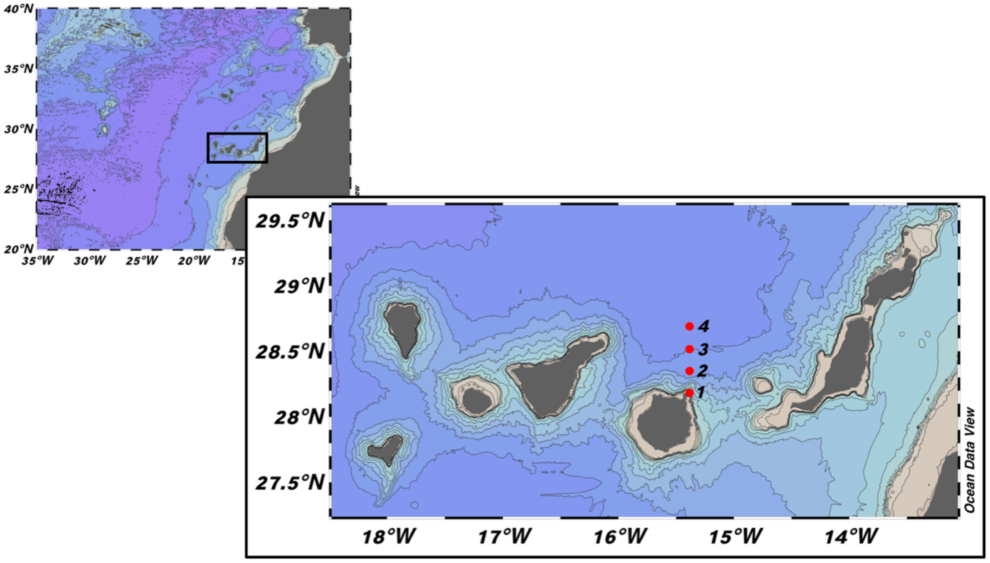
Figure 1. Location of the four sampling stations (red dots) at the North of Gran Canaria Island, Canary Islands.

On board, one of the cod-ends from the double WP-2 net was sieved into 100-200, 200-500, 500-1000, 1000-4000, and >4000 μm size fractions. Samples were then frozen in liquid nitrogen (-196°C) for subsequent analysis of gut fluorescence (GF), electron transfer system (ETS) and aminoacyl-tRNA synthetase (AARS) activities. The zooplankton sample from the other cod-end was preserved at 4°C in formaldehyde (1%) for less than 24 hours to avoid a decrease in dry weight and split in the laboratory the following day to obtain the total biomass and abundance of zooplankton.

2.2 Chlorophyll a, pico-, nano-, microplankton, and primary production

Samples for chlorophyll a concentration were taken at 20 m depth as representative of the mixed layer (see Armengol et al., 2020), filtered (500 mL) through a 25 mm Whatman GF/F, and stored at -20°C. In the laboratory, the filter was placed in 90% acetone at -20°C in the dark for 20 hours (Strickland and Parsons, 1972). Pigments were measured using a Turner Design 10A Fluorometer, previously calibrated with pure chlorophyll a (Yentsch and Menzel, 1963).

Pico-, nano-, and microplankton biomass were published in Armengol et al. (2020) and we used this data to compare with our results about zooplankton abundance, biomass, and metabolic proxies. Samples were also obtained at 20 m depth. Briefly, 0.2-2 µm picoplankton (Picoeukaryotes, Synechococcus, and Prochlorococcus) were counted by flow cytometry (FACScalibur cytometer). Samples of 45 ml were used to count nanoplankton (2-20 µm, autotrophic and heterotrophic nanoflagellates) and they were fixed with glutaraldehyde, stained with DAPI, and counted by epifluorescence microscopy with a Zeiss Axiovert 35 microscope. Samples of 500 ml were obtained for microplankton (>20 µm, diatoms, silicoflagellates, dinoflagellates, ciliates, and copepod nauplii), fixed with acid Lugol’s iodine and aliquots of 100 mL of sample were placed in Utermöhl sedimentation chambers for 48 h, and counted using a Zeiss Axiovert 35 inverted microscope. Microplankton was also sampled at 20 m depth but only in Station 3 as representative of oceanic conditions. All abundance data were converted to biomass using different published conversion factors (see Armengol et al., 2020 for details).

Primary production data were obtained from the Ocean Productivity web site (http://www.science.oregonstate.edu/ocean.productivity/index.php) based on remote sensing data following Behrenfeld and Falkowski (1997), and using the Vertical Generalized Production Model (VGPM).

2.3 Zooplankton biomass and abundance

Zooplankton biomass was obtained from dry weight following the procedure given by Lovegrove (1966). The sample was dried for 24 hours at 60°C and later weighed on a microbalance. The other half of the zooplankton sample was used for abundance estimations. For this, digital images of the samples were obtained using an Epson Perfection 4990 Photo scanner (with VueScan Professional Edition 8.4.77 software). Samples were size-fractionated through a 1-mm mesh net. To obtain clear digital images, an aliquot of each subsample was taken with a Hensen pipette and placed into a polystyrene plate to be scanned at a resolution of 1200 dpi. The images were processed using the ZooImage 1 version 1.2-1 software (http://www.sciviews.org/zooimage) according to the method used by Grosjean and Denis (2007). A manual training set was performed to help the software automatically classify major taxa. Categories included were copepods, chaetognaths, gelatinous organisms (doliodids, salps, siphonophores, hydromedusae), and other zooplankton (mostly ostracods, polychaetes larvae, amphipods, zoea larvae of decapods, adult polychaetes, and stomatopod larvae). We also distinguished euphausiids, mysids, and mysis larvae of decapods in another group as they have a similar shape recognized by the software.

2.4 Gut fluorescence, ETS and AARS activities

In the laboratory, frozen zooplankton samples previously stored in liquid nitrogen were homogenized with Tris-HCl buffer (pH=7.8), and different subsamples were taken for gut fluorescence measurements, ETS and AARS activities. The protein content was determined using the Folin dye method based on Lowry et al. (1951) and modified by Rutter (1967) using bovine serum albumin (BSA) as standard.

An aliquot of the homogenized sample was used for gut fluorescence analyses, and it was placed in a test tube with 10 mL of 90% acetone and stored at -20°C for 24 hours in darkness. Fluorescence of samples was measured before and after acidification with 3 drops of 10% HCl in a Turner Design fluorometer (model 10-AU-005-CE), previously calibrated with pure chlorophyll a as described by Yentsch and Menzel (1963). Pigments were calculated following Strickland and Parsons (1972), modified by Hernández-León et al. (2001b) for homogenate samples, and then normalized to the protein content of the sample using the following equations:

$$\text{Chlorophyll\hspace{0.33em}}a=k·(F_o-F_a){\text{mg}}^{-1}\text{\hspace{0.33em}protein}$$

$$\text{Pheopigments}=k·(\text{R}\text{'}{F}_o-F_a){\text{mg}}^{-1}\text{\hspace{0.33em}protein}$$

where k is the instrument calibration constant, F_o and F_a are the fluorescence readings before and after acidification, and R is the acidification coefficient. Chlorophyll a and phaeopigments values were added to obtain specific GF.

Another subsample of the homogenate was incubated at 18°C for ETS activity following the method of Packard (1969) modified by Kenner and Ahmed (1975) for zooplankton samples. Details of the procedure are given by Hernández-León and Gómez (1996). ETS activity was corrected for in situ temperature using the Arrhenius equation and an activation energy of 15 Kcal mol^-1 (Packard et al., 1975).

Aminoacyl-tRNA synthetase (AARS) activity was measured following the method of Yebra and Hernández-León (2004), modified by Yebra et al. (2011), and calculated using the equation given by Herrera et al. (2017). The enzymatic activities were recalculated for the in situ temperature using the Arrhenius equation and the corresponding activation energies for AARS (8.57 kcal mol^-1, Yebra et al., 2005). Finally, ETS and AARS activities were normalized according to the protein content of the sample to compare the different size fractions.

2.5 Statistical analysis

Chlorophyll a differences between stations were tested using a two-way analysis of variance (ANOVA). Normality was tested using the Shapiro-Wilk test, and homoscedasticity was tested using the Bartlett test. For zooplankton abundance, biomass, gut fluorescence, specific ETS activity, and specific AARS activity, a two-way analysis of variance (ANOVA) approach was applied to assess the effect of the factor stations (with four levels) and the factor size-fraction (with five levels). Each dataset (i.e., biomass, gut fluorescence, specific ETS, and AARS activities) were transformed as necessary to meet ANOVA assumptions of normality of the distribution and homoscedasticity. Data were transformed using the Box-Cox power transformation. Normality and homoscedasticity were tested as mentioned above. Provided a significant effect of a given factor, the main effects for this factor within each level of the other were further inspected using the post hoc Duncan test. All analyses considered an alpha level of 0.05.

In order to identify patterns related to the lunar cycle, the different variables were plotted using a non-parametric local polynomial regression model (LOESS, Cleveland and Devlin, 1988; Cleveland et al., 1988). The non-parametric regression LOESS technique that fits multiple regressions in local neighborhood provides a robust fitting when there are outliers in the data. In this context, non-parametric means that no assumptions need to be made about the underlying distribution (form) of the data (Jacoby, 2000). Fitting was done locally, that is for the fit at point x, the fit is made using points in a neighborhood of x, weighted by their distance from x (with differences in “parametric” variables being ignored when computing the distance). The size of the neighborhood was controlled by α (span), i.e. the proportion of all data that is to be used in each local fit (size of neighborhood of x). Here, we used α = 0.6 for all fits, so, each of the local regressions used to produce that curve incorporates 60% of the total data points. This was proved to be a suitable compromise between smoothing and preserving of temporal structural information. Linear regression analysis was used to check if the residuals from the LOESS fits adequately incorporates all the interesting structure in the data (Jacoby, 2000). Finally, to model the lunar cycle, we applied the obtained LOESS model to a sequence of numbers according to the lunar illumination from 0 (new moon) to 1 (full moon). The validation of the loess model was conducted by comparing it to a null model using an ANOVA approach. Specifically, a LOESS model was fitted to the data, and a null model (intercept-only) was also fitted for comparison. An analysis of variance (ANOVA) was then performed to compare these models. The F-value and p-value obtained from the ANOVA were used to assess the significance and performance of the LOESS model. Analyses were performed using the LOESS algorithm implemented in the Stats package of R, version 2023.06.1 + 524 (R Core Team, 2022).

3 Results

3.1 Hydrography and primary production

Temperature in the mixed layer (Figure 2A) showed higher values during November and December (above of 21°C), decreasing during January and February, and reaching the lowest values during March (below 19°C). Convective mixing started at the end of January and beginning of February and stratification started during April. These changes were also observed in salinity (Figure 2B), resulting in a weak chlorophyll bloom during March (Figure 2C).

Figure 2

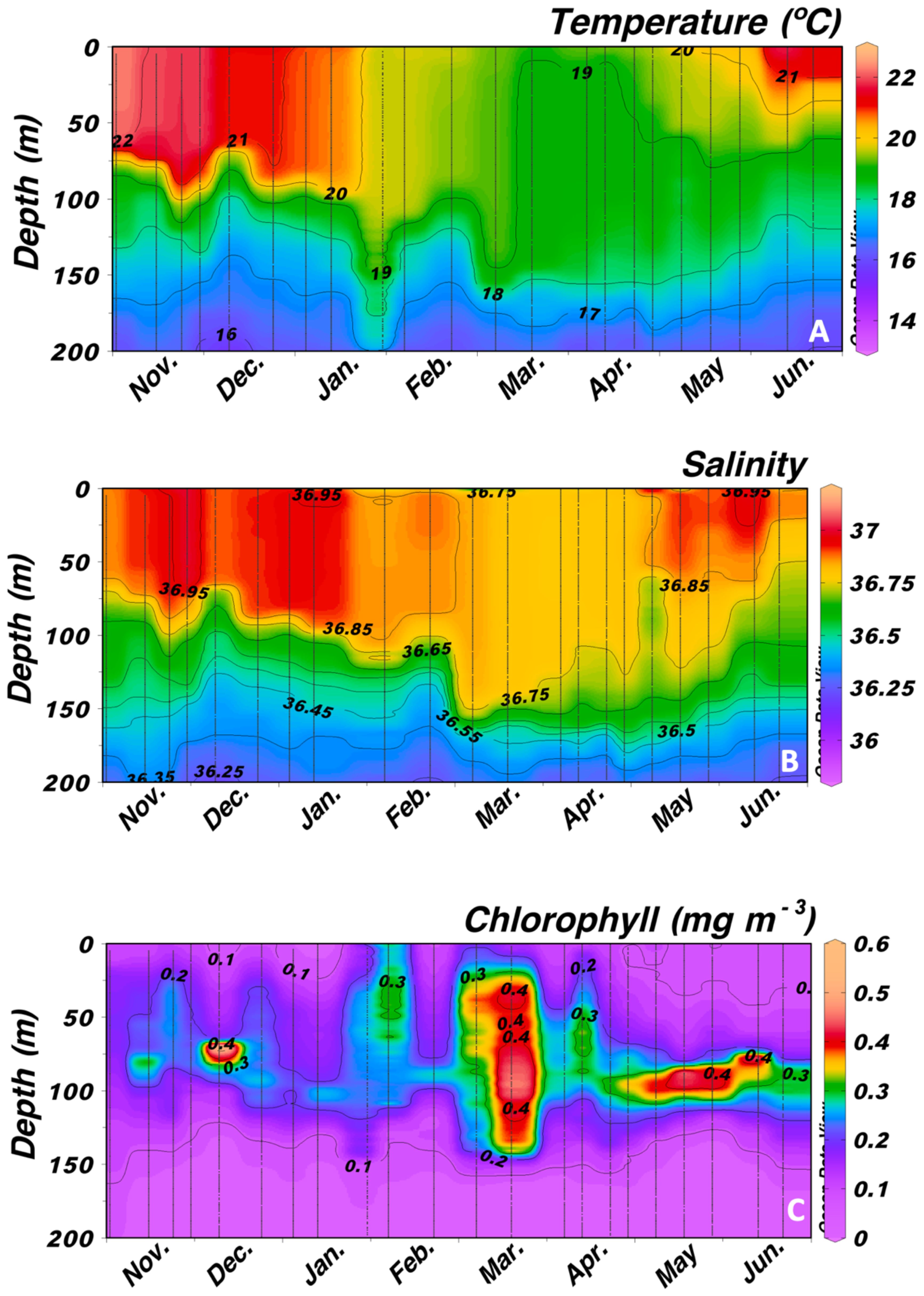
Figure 2. Vertical distribution of (A) temperature (°C), (B) salinity, and (C) chlorophyll a (mg m^-3) from surface to 200 m depth at Station 3.

Primary production obtained from remote sensing (Figure 3A) increased during February and remained high until the beginning of April reflecting the mixing period observed in temperature and salinity. However, average values for chlorophyll a at 20 m depth (Figure 3A) showed low values throughout the period of study, as expected in a subtropical oceanic site, peaking at almost monthly intervals. Average values of chlorophyll a in the mixed layer also displayed low values as expected, peaking at monthly intervals related to the lunar cycle (Figure 3B, see below) as also observed visually in Figure 2C.

Figure 3

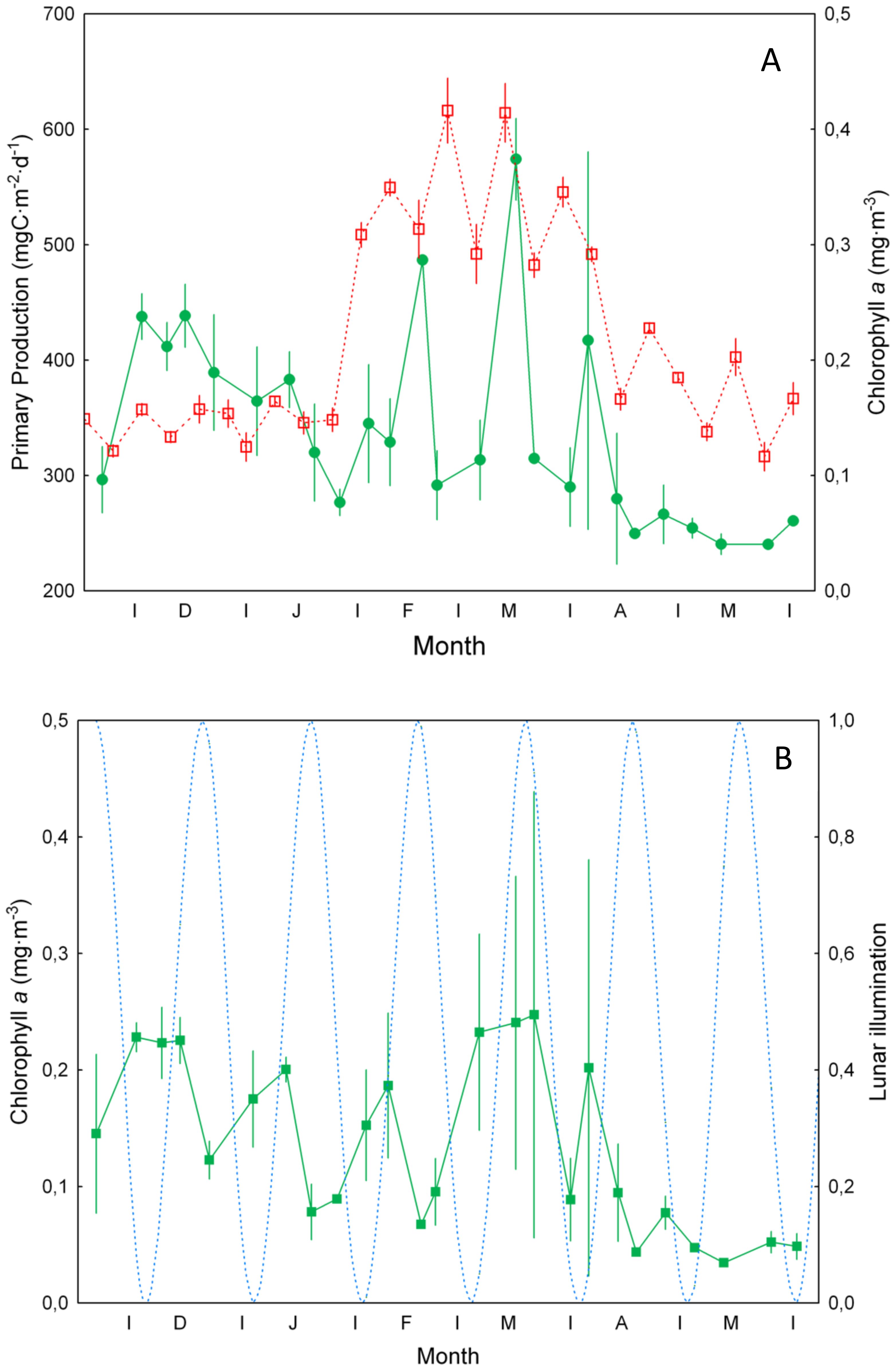
Figure 3. (A) Primary production (±SE, mg C m^-2 d^-1) (in red) as observed from remote sensing, and average chlorophyll a concentration (±SE, mg m^-3) (in green) at 20 m depth. (B) Average (±SE) values of chlorophyll a concentration (mg m^-3) in the mixed layer. Dashed blue line is the potential lunar illumination (0 is new moon and 1 is full moon).

3.2 Zooplankton abundance, biomass, and physiological indices

Zooplankton abundance was significantly higher (ANOVA test, p<0.001) in the 200-500 µm size fraction (Figure 4A). Average values of abundance in all size classes (Figure 4B) followed the trend of the 200-500 µm size fraction. We also observed significantly higher values (ANOVA test, p<0.001) of zooplankton biomass in the 1000-4000 µm size class during the late winter bloom (Figure 5A). By opposite, the lower average values were observed in the >4 mm size fraction followed by the 100-200, 200-500, and 500-1000 µm size classes. Copepods were the most representative zooplankton group in terms of biomass (>71.5%) and other groups such as chaetognaths (3.6-22%), and other crustaceans (0.3-17%) were also important (Supplementary Figure S1). Total zooplankton biomass (Figure 5B) followed the trend of the 1000-4000 µm size fraction and peaked during February and March, the period of maximum convective mixing in the water column. No significant relationship was observed between total biomass and the lunar cycles during the whole period of study (Spearman correlation r² = 0.017, p>0.05).

Figure 4

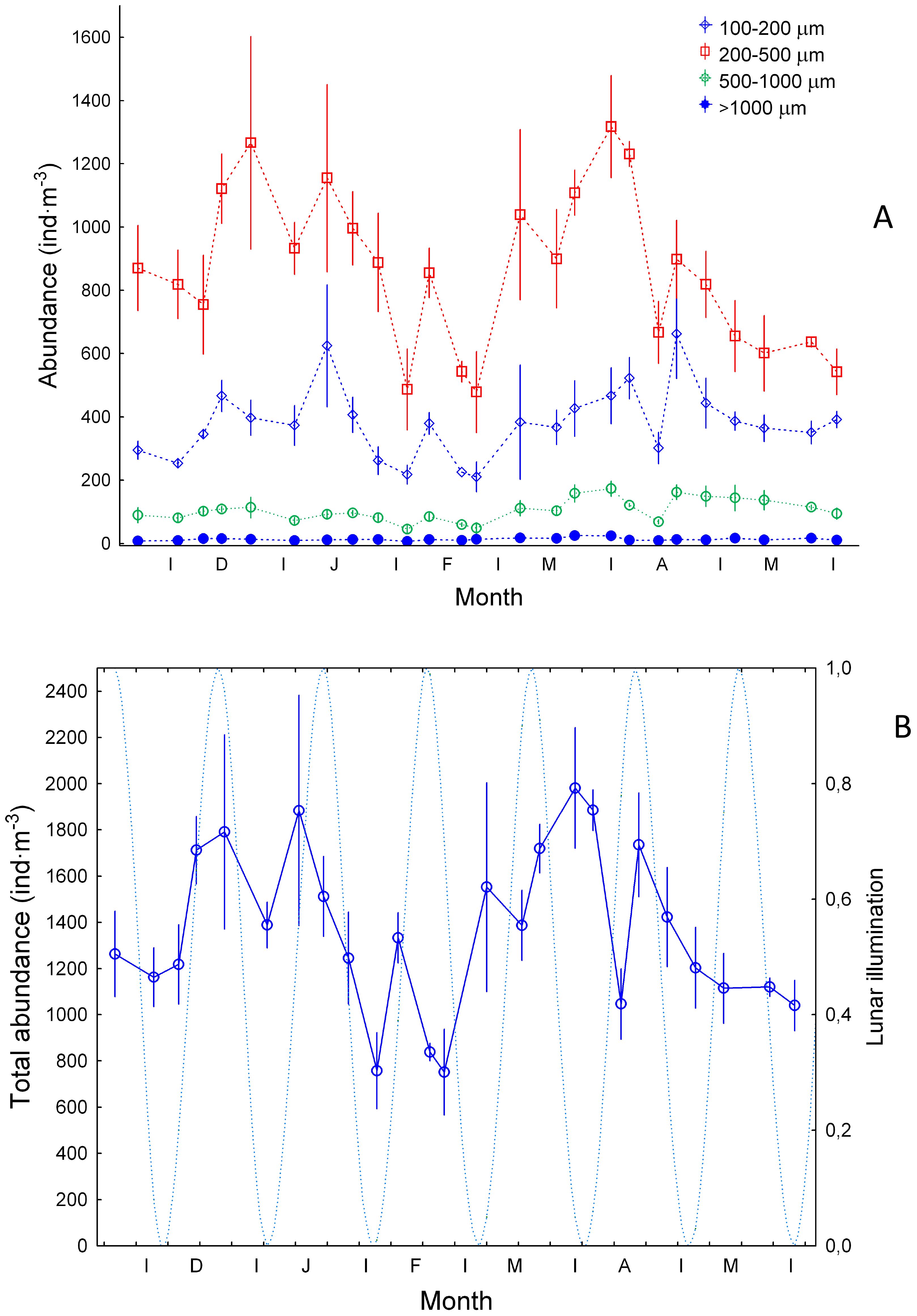
Figure 4. Zooplankton abundance (ind m^-3, ±SE) (A) for size ranges of 100-200 µm, 200-500 µm, 500-1000 µm and >1000 µm, and (B) from 100 to >1000 µm. “Ind” stands for individuals. Dashed blue line and lunar illumination as in Figure 3.

Figure 5

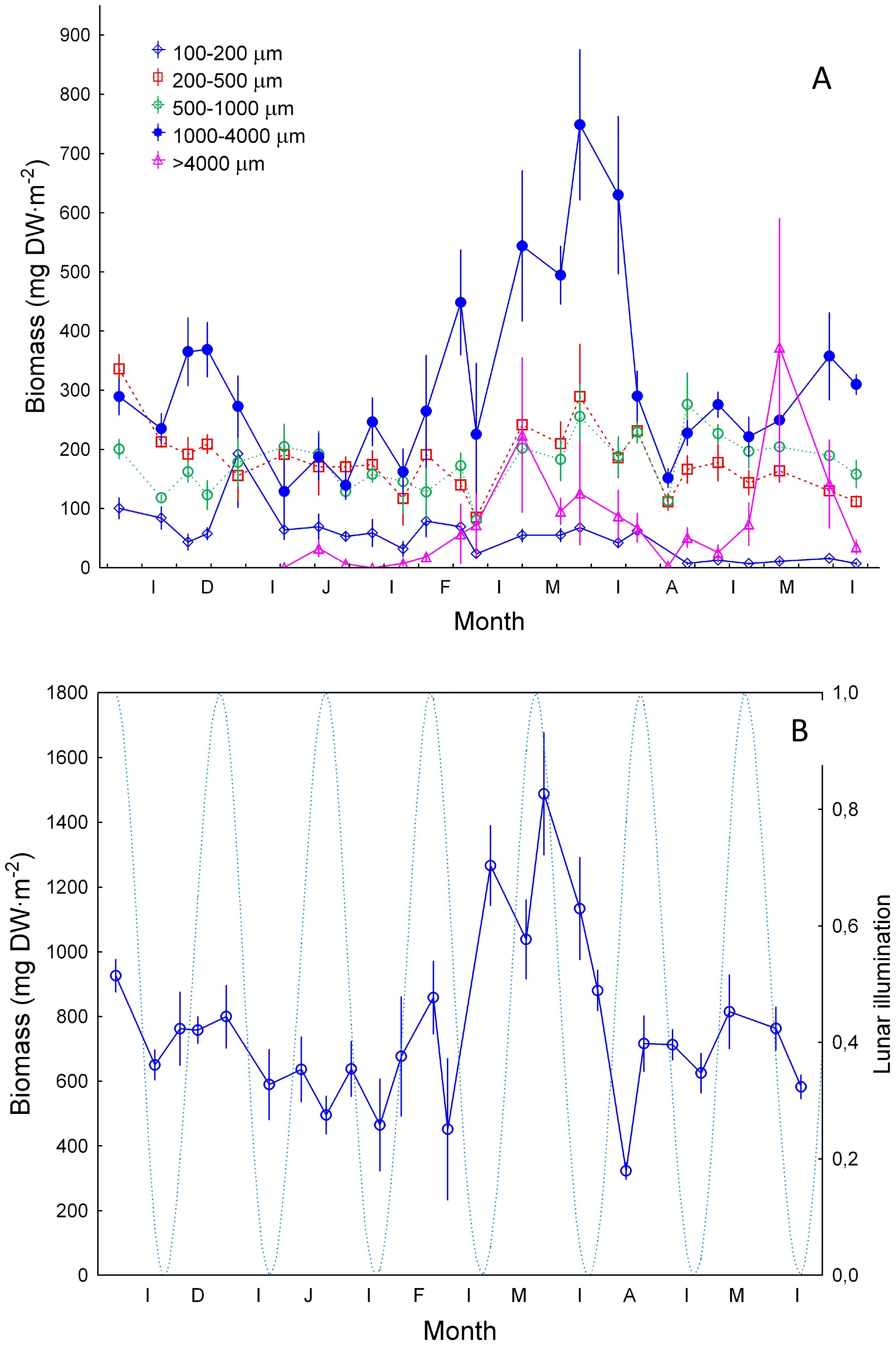
Figure 5. Zooplankton biomass (mgDW m^-2, ±SE) (A) for size ranges of 100-200 µm, 200-500 µm, 500-1000 µm and >1000 µm; and (B) from 100 to >1000 µm. DW stands for dry weight. Dashed blue line and lunar illumination as in Figure 3.

Average values of size-fractionated specific gut fluorescence (Figure 6A) showed a rather large variability and varied among size fractions (ANOVA test, p<0.05). The highest average values of specific GF were found in the smaller size class (100-200 µm) throughout the period studied as expected from the smaller size of phytoplankton in oligotrophic waters. Peaks of GF were also observed in the other size fractions. Average values (Figure 6B) showed increases in GF at almost monthly intervals. Station 1 was not considered here as it displayed significant differences with the other stations.

Figure 6

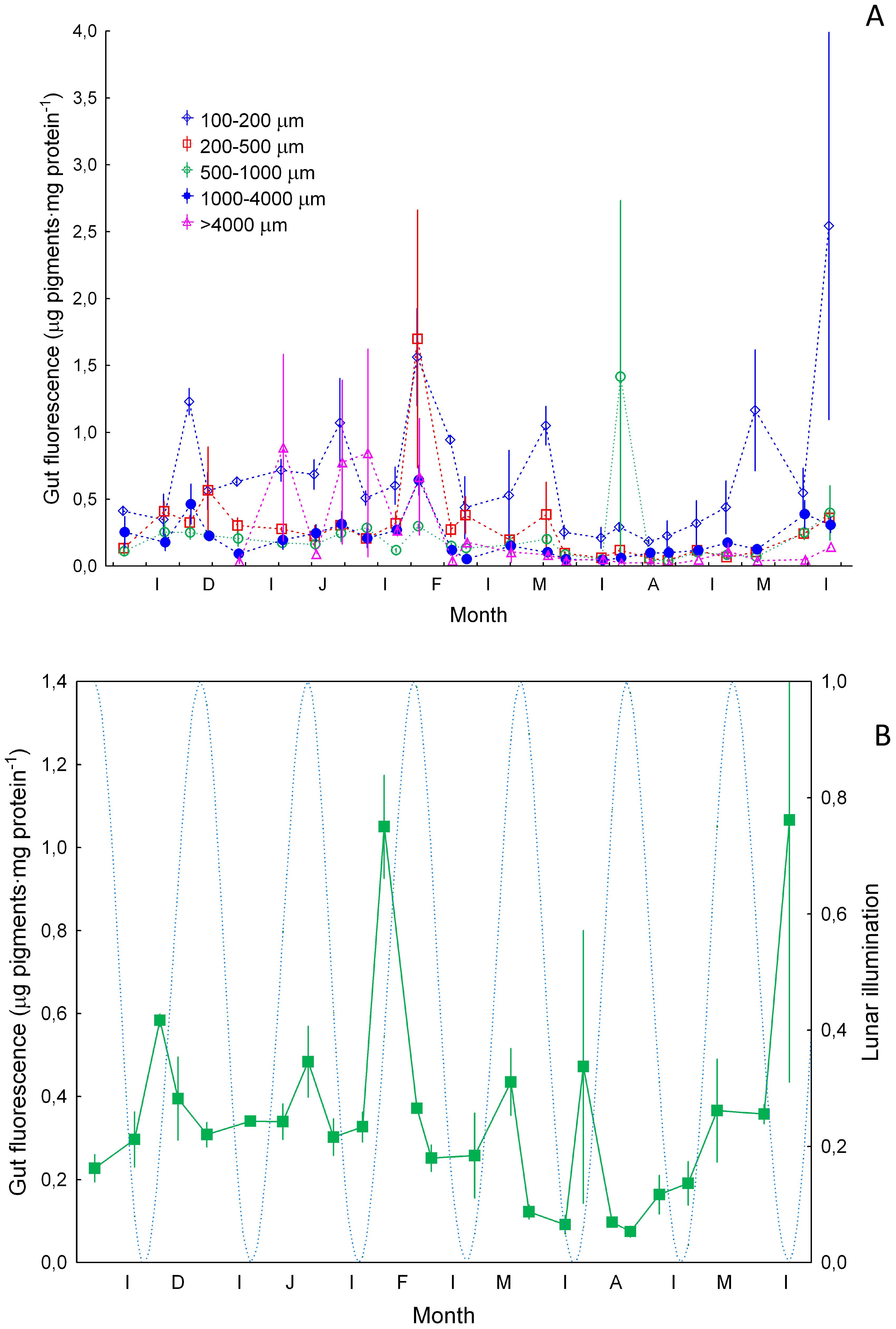
Figure 6. Specific gut fluorescence (µg pigments·mg protein^-1, ±SE) (A) for zooplankton size ranges of 100-200 µm, 200-500 µm, 500-1000 µm and >1000 µm, and (B) average values (±SE). Dashed blue line and lunar illumination as in Figure 3.

Large variability was also observed in specific ETS activity (Figure 7A) with the 200-500 and 500-1000 µm size fractions showing significantly higher values (Kruskal-Wallis, p<0.05) than the large (>1000 µm) and small (100-200 µm) zooplankton. Increases observed in each size fraction did not show significant differences before, during, and after vertical mixing (Kruskal Wallis p>0.05). Average values varied less than gut fluorescence along the period studied (Figure 7B). Station 1 was also not considered here as it displayed significant differences with the other stations.

Figure 7

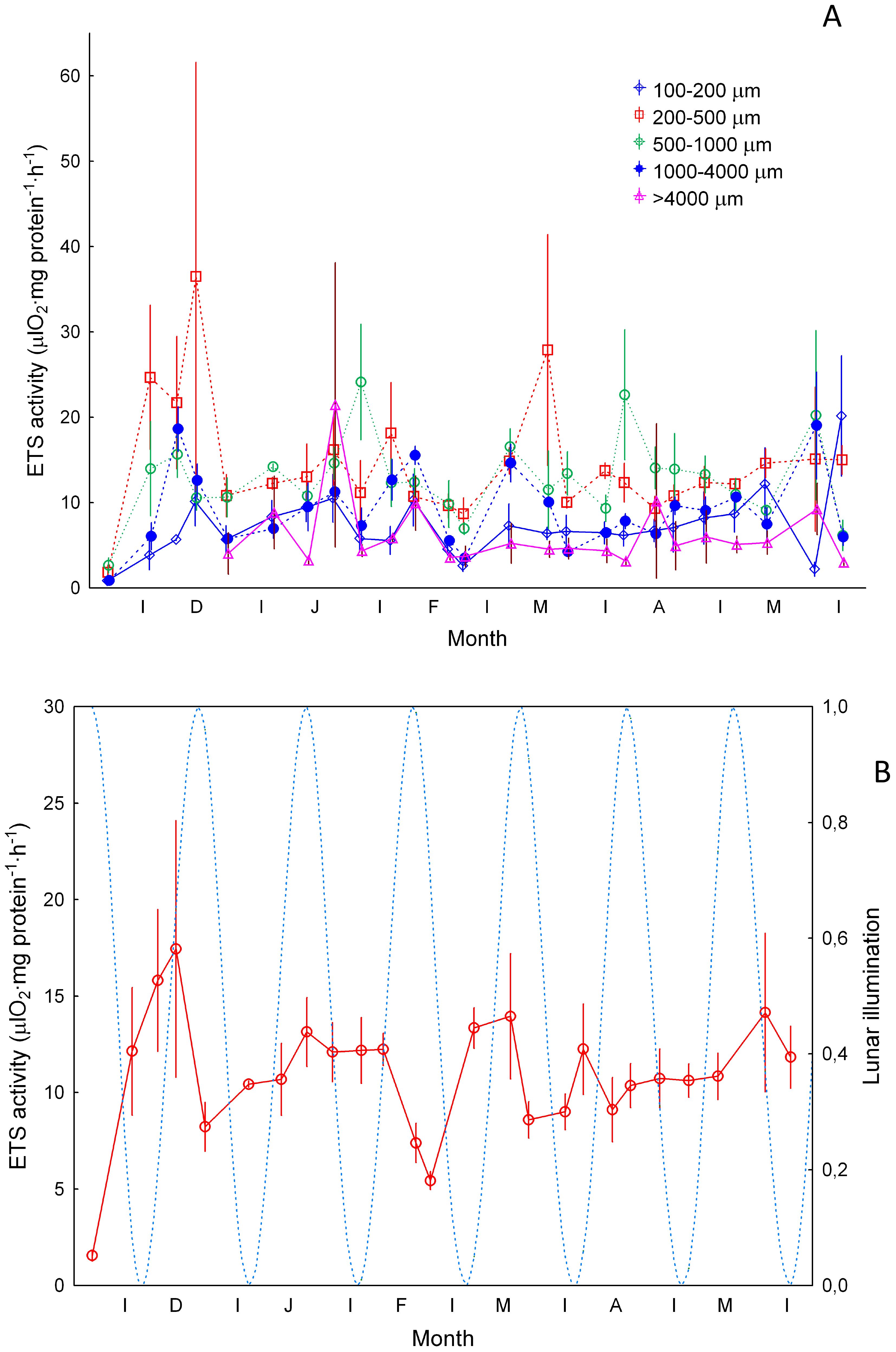
Figure 7. Specific ETS activity (µlO₂·mg protein^-1·hour^-1, ±SE) (A) for zooplankton size ranges of 100-200 µm, 200-500 µm, 500-1000 µm and >1000 µm, and (B) average values (±SE). Dashed blue line and lunar illumination as in Figure 3.

Specific AARS activity showed considerable variability in the 100-200, 200-500, and >1000 µm size fractions (Figure 8A). The highest average values (>140 nmol PPi·mg protein^-1·h^-1) were found in the small size fraction (100-200 µm) as expected from the higher specific growth of smaller individuals. Zooplankton >500 µm showed higher average values in January and April (before and after the bloom), while the 200-500 µm fraction showed increases during December (113 ± 80.8 nmol PPi·mg protein^-1·h^-1) and March (119± 53 nmol PPi·mg protein^-1·h^-1). Average values showed sharp increases at monthly intervals peaking just before the full moon (see below), suggesting a match with the lunar cycle (Figure 8B).

Figure 8

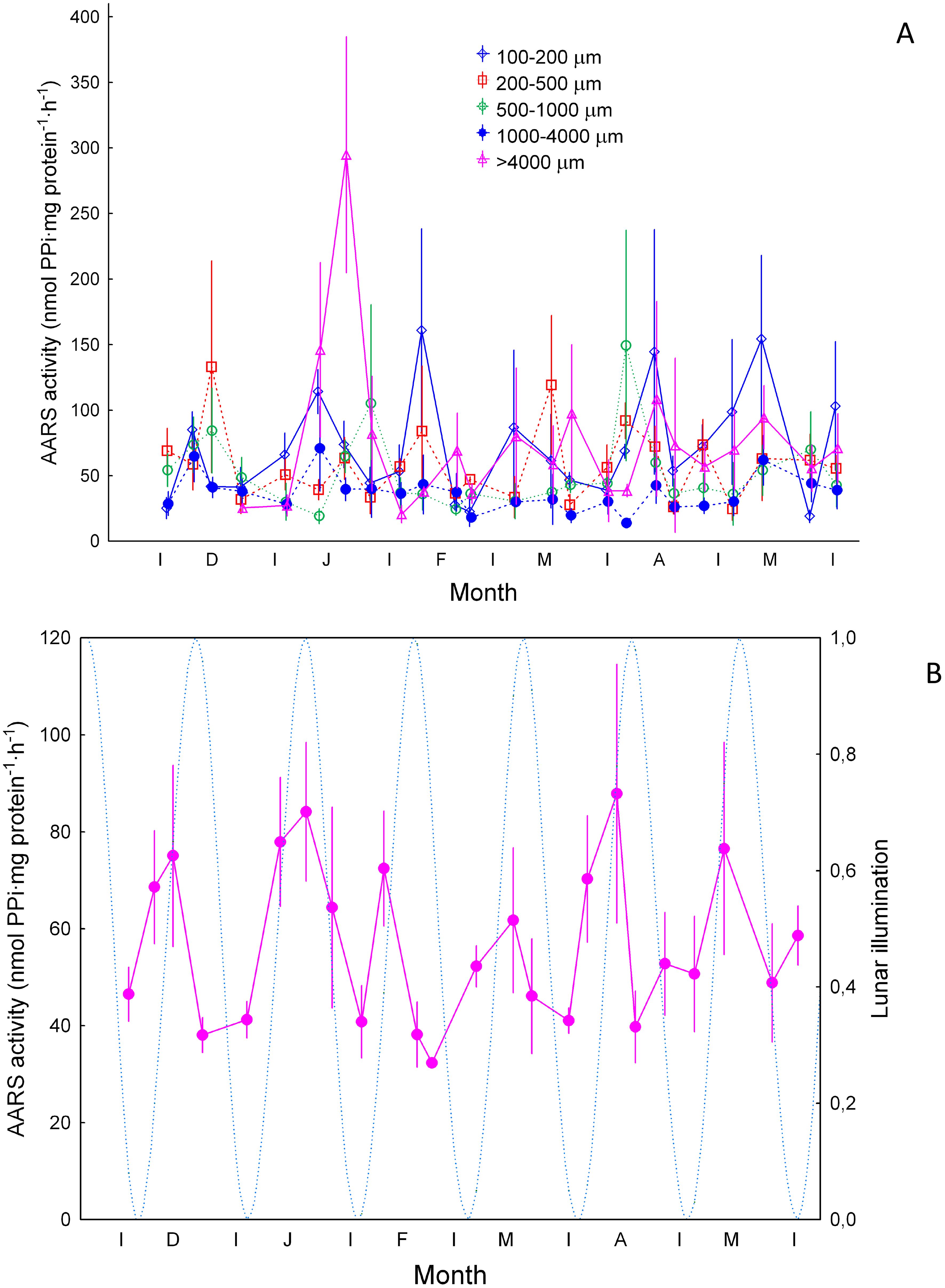
Figure 8. Specific AARS activity (nmol PPi·mg protein^-1·h^-1, ±SE) (A) for zooplankton size ranges of 100-200 µm, 200-500 µm, 500-1000 µm and >1000 µm, and (B) average values (±SE). Dashed blue line and lunar illumination as in Figure 3.

3.3 Lunar cycle patterns

In order to identify patterns related to the lunar cycle, we used a local regression model (LOESS) to detrend the data, achieving a robust parametrization of the different biological variables, in order to unveil the monthly variability observed and its relationship with the lunar cycle. The smoothing function of the model showed an increase of chlorophyll a just after new moon in the upper 0-70 m layer (Figure 9A). According to the model, the chlorophyll a maximum was reached between 5 and 6 days after the new moon (ANOVA test, F-value= 7.48, p-value=0.006). Model results for deeper layers are shown in Supplementary Figure S2. We observed statistical differences in picoplankton between Station 1 and the other (ANOVA test, F-value=6.75, p-value=0.01), so this station was excluded from the analysis. We did not find a significant match of picoplankton organisms with the lunar cycle (Supplementary Figure S3A) (ANOVA test, F-value= 0.007, p-value=0.9), nor with dinoflagellates (ANOVA test, F-value= 0.107, p-value=0.75) and ciliates (Supplementary Figure S3B) (ANOVA test, F-value= 0.59, p-2value=0.45). However, we observed a striking pattern with nano- and heterotrophic nanoplankton (Figure 9B) and diatoms (Figure 9C), similar to chlorophyll a. Modelled zooplankton abundance (Figure 10A) (ANOVA test, F-value=0.09, p-value=0.76). and biomass (Figure 10B) (ANOVA test, F-value=3.47, p-value=0.06) showed no relationship with the lunar cycle.

Figure 9

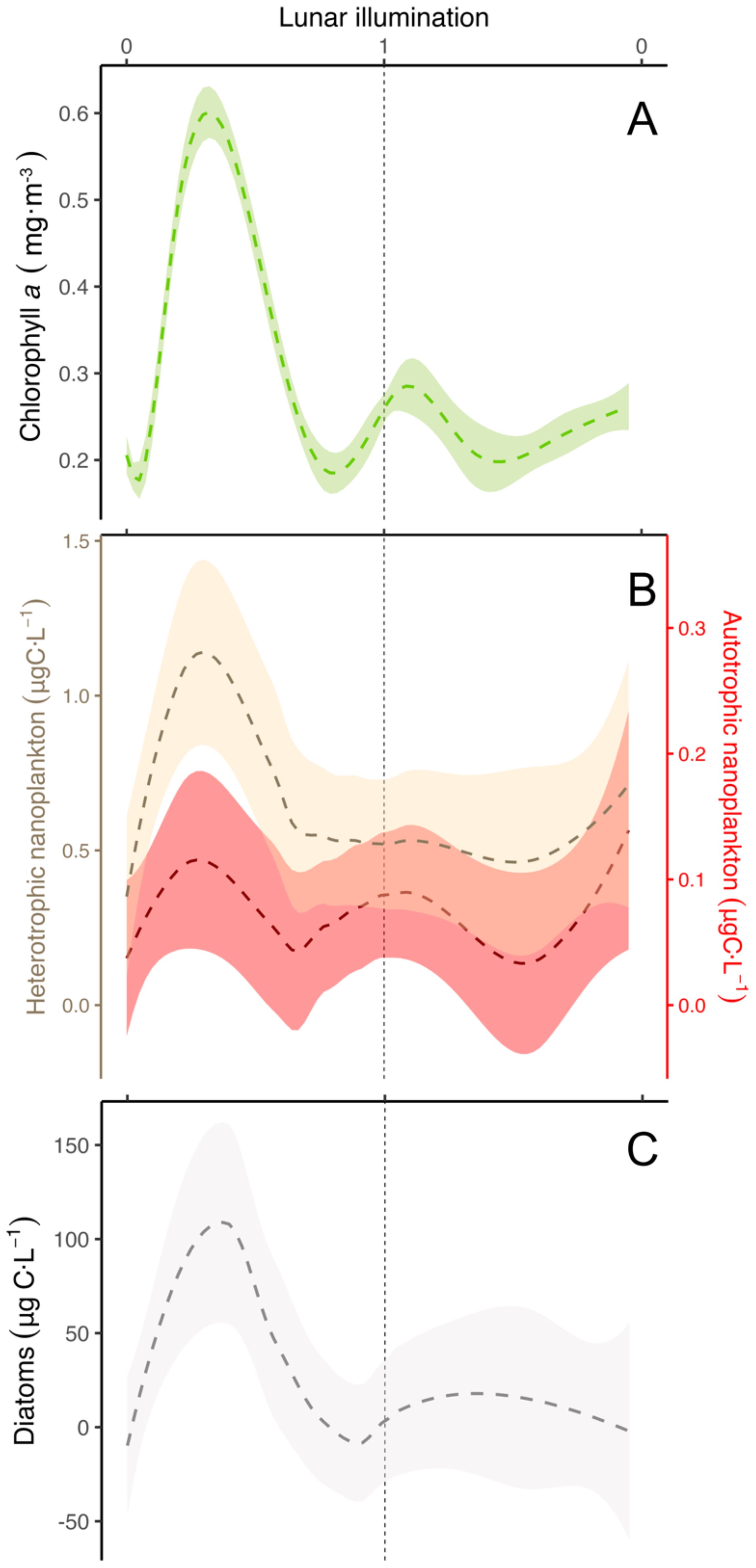
Figure 9. Modelled lunar cycle using the LOESS method (colored dashed lines) for (A) chlorophyll a in the upper 0-70 m layer, (B) autotrophic and heterotrophic nanoflagellates, and (C) diatoms. Vertical dashed black line stands for the full moon (lunar illumination of 1). The shadowed area corresponds to the span (see material and methods).

Figure 10

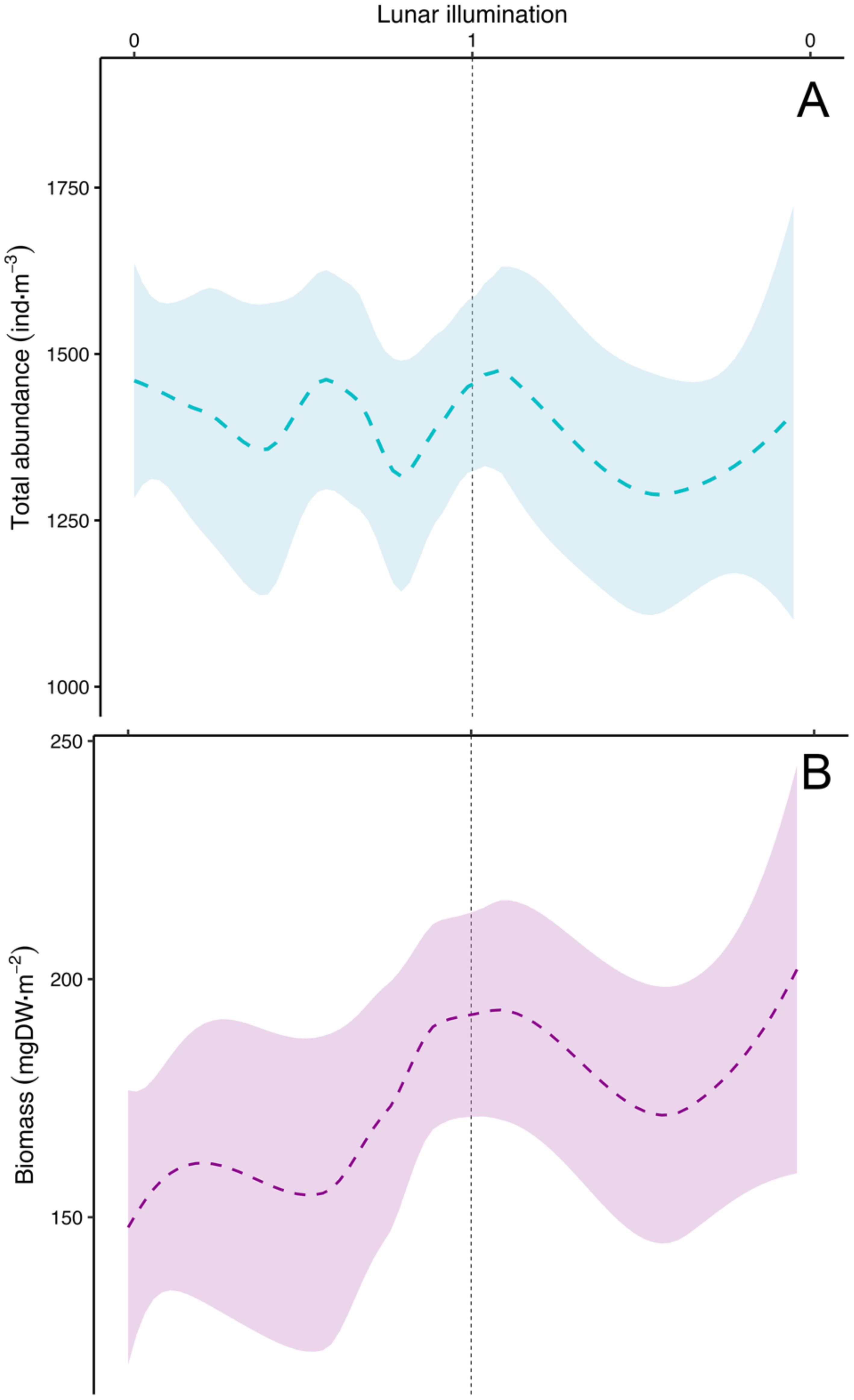
Figure 10. Modelled lunar cycle using the LOESS method (as in Figure 9) for total zooplankton (A) abundance (ind m^-3) and, (B) biomass (mg DW m^-2). Vertical dashed black line stands for the full moon (lunar illumination of 1). Shadowed area as in Figure 9.

Significant differences were found in the zooplankton gut fluorescence between stations (ANOVA test, F value = 3.78, p-value <0.05) and, according to the Duncan test results, Station 1 was not considered when modeling the lunar cycle to avoid significant differences between this and the other stations. The gut fluorescence lunar cycle model (Figure 11A) showed the peak occurring between 4 to 6 days after the new moon, coinciding with a lunar illumination between 0.25-0.35 (0 for the new moon and 1 for full moon). The results of the Duncan test for zooplankton specific ETS activity showed significant differences between Station 1 and Stations 2-4. Thus, Station 1 was not considered when modelling the zooplankton specific ETS activity (Figure 11B). The maximum specific ETS activity values over the lunar cycle were obtained coinciding with the gut fluorescence and a lunar illumination between 0.3-0.35 (i.e., 5 to 6 days after the new moon). Finally, no significant differences were found between stations for zooplankton specific AARS activity (ANOVA test, F-value=1.18, p-value= 0.317) (Figure 11C). According to the model fitted to the specific AARS activity values, the maximum activity was obtained 8 to 9 days after the new moon, coinciding with a lunar illumination of 0.5 to 0.6.

Figure 11

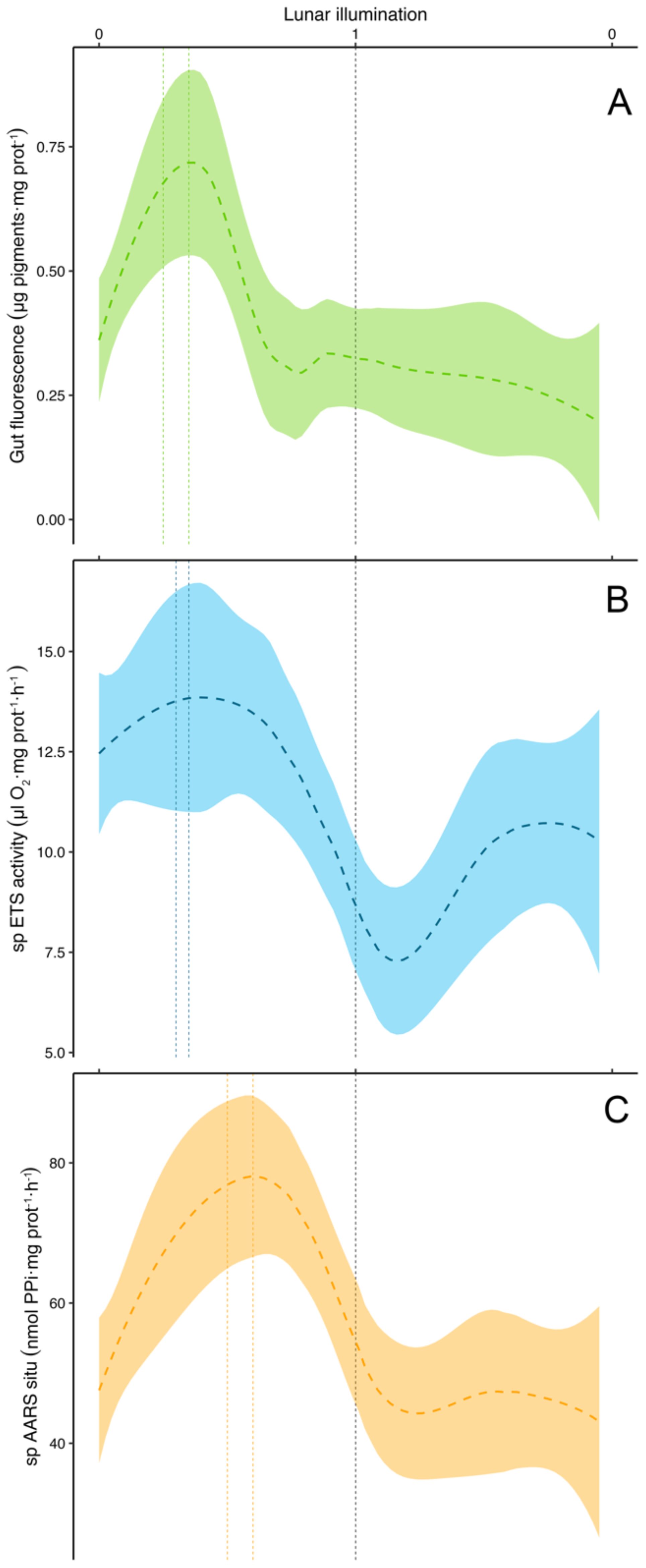
Figure 11. Modelled lunar cycle using the LOESS method (as in Figure 9) for (A) gut fluorescence (µg pigments·mg protein^-1), (B) specific (sp) ETS activity (µlO₂·mg protein^-1·h^-1), and (C) specific (sp) AARS situ (nmol PPi·mg protein^-1·h^-1). Vertical black line stands for the full moon (lunar illumination of 1), and dashed colored vertical lines represent the period of maximum activity. Shadowed area as in Figure 9.

4 Discussion

4.1 Plankton variability during the late winter bloom

Short-term variability of phyto-, micro-, and mesozooplankton were scarcely studied in the subtropical oligotrophic ocean mainly due to logistical problems related to the access to these normally remote areas, the important effort required to sample at least every week in the open ocean, and the high economic cost of long-term sampling (several months). These constraints force the use of small boats for sampling in rough seas, particularly in Trade Wind zones. This short-term variability is also of importance in warm oligotrophic waters as temperature induce faster plankton turnover rates. Also, the study of lunar cycles has attracted many researchers working in coral reefs (Fan et al., 2002), fish larvae (Shima and Swearer, 2019), and zooplankton (Gliwicz, 1986; Roura et al., 2013). Hernández-León (1998) observed a lunar cycle in zooplankton in open waters around the Canary Islands showing an increase of zooplankton abundance which was subsequently evidenced for biomass (Hernández-León et al., 2001a, 2002, 2004, 2010).

However, the increase in zooplankton biomass was mostly related to the late winter bloom, varying with the length of convective mixing and the productive bloom. Several authors observed the typical planktonic outburst during the winter vertical mixing when temperature fell below 18°C in the Canary Current (De León and Braun, 1973; Braun, 1980; Hernández-León et al., 2004; Moyano et al., 2009; Hernández-León et al., 2010; Schmoker et al., 2012). The relatively lower temperature during late winter promoted a sharp phytoplankton bloom as stated above. In these previous studies on coastal and oceanic blooms, chlorophyll a ranged from 0.5 to 1.0 mg·m^-3 (Arístegui et al., 2001; Hernández-León et al., 2004; Moyano et al., 2009; Neuer et al., 2007; Schmoker et al., 2012, 2014). Colder years showed large chlorophyll a values (Neuer et al., 2007; Schmoker et al., 2014) because the cooling of surface waters promoted mixing below 100 m and an increase in nutrient flux (Cianca et al., 2007).

Differences in the duration of the phytoplankton bloom were related to the shorter or larger effect of temperature and convective mixing as evidenced by Schmoker and Hernández-León (2013). In our study, chlorophyll a values in the mixed layer were quite low (around 0.3 mg m^-3) and similar to the range given by Schmoker and Hernández-León (2013) during the mild and warm winters of 2006 and 2007, respectively. However, these values were higher than those found by Herrera et al. (2017) and Armengol et al. (2020) during the extremely warm year of 2010 (maximum of about 0.1 mg·m^-3 at 20 m depth). In the latter studies, the high temperature during 2010 restricted the vertical flux of nutrients to the euphotic zone limiting phytoplankton growth.

Our study, conducted during 2011 which was neither a warm, nor a cold year (mixed layer temperature was 18-19°C) did not promote a large phytoplankton bloom (Armengol et al., 2020). We observed an increase in zooplankton biomass with two peaks, a small one during February and the most important during March (Figure 5B). Zooplankton biomass during this warm winter was also lower than in previous years in oceanic waters north of the Canary Islands (see Hernández-León et al., 2004). During colder winters in these subtropical waters, two or three zooplankton biomass increases were normally observed between January and May (see Schmoker and Hernández-León, 2013), although they varied and were not always observed during the same period. Some studies reported zooplankton outburst in February and March (Arístegui et al., 2001; Hernández-León et al., 2004, 2010; Schmoker and Hernández-León, 2013; Schmoker et al., 2014), while others observed these blooms during March and April, or even in May after the phytoplankton bloom (Moyano et al., 2009; Schmoker et al., 2012; Couret et al., 2023). Between 2005 and 2007, Schmoker and Hernández-León (2013) observed a rather clear interannual variability of zooplankton biomass related to temperature during the vertical mixing period. The bloom was shorter during warm years suggesting that differences in temperature of only 0.5°C during the vertical mixing period could cause important changes in the pelagic ecosystem structure of subtropical waters. They found an increase in zooplankton biomass over three months during a cold winter (2005), while it lasted less than one month during a warm year (2007). In our study, the low values of zooplankton biomass related to the low chlorophyll and primary production during this relatively warm winter should be the tentative explanation for the absence of several zooplankton biomass peaks at monthly intervals during this winter. These lower biomass values contrasted with years of high (Hernández-León et al., 2010) or medium values (Hernández-León et al., 2004).

4.2 Planktonic variability during the lunar cycle

Lunar cycles in zooplankton abundance (Hernández-León, 1998) and biomass (Hernández-León et al., 2001a, 2002, 2004, 2010) were identified in previous studies during the late winter bloom. In our study, we observed a consistent lunar cycle (LOESS function) in chlorophyll a (Figure 9A), auto- and heterotrophic nanoplankton (Figure 9B), and diatoms (Figure 9C). However, this pattern was not evident in zooplankton abundance (Figure 10A) or biomass (Figure 10B) considering all the sampled period. Zooplankton gut fluorescence (ANOVA test, F-value=6.99, p-value=0.008), ETS (ANOVA test, F-value=6.32, p-value=0.01), and AARS activities (ANOVA test, F-value=1.88, p-value=0.17) (Figure 11) showed a significant, except for the AARS activities, increase before full moon, despite the presence or not of an increase in zooplankton biomass. This pattern was easily observable during most of the lunar cycles (see Figures 6–8). Thus, chlorophyll a (Figure 9A), auto- and heterotrophic nanoplankton (Figure 9B), diatoms (Figure 9C), and the metabolic functioning of zooplankton (Figure 11) showed a lunar pattern at the short-term, but not for zooplankton abundance and biomass.

Schmoker et al. (2012) observed pico-, nano-, and microplankton following a lunar cycle during their weekly study around the Canary Islands (see their Figure 6). They found an increase in picoplankton coinciding with the zooplankton peak, followed by an increase in nano-, and microplankton. The parallel increase of pico- and zooplankton was explained as the control exerted by the latter community upon microplankton releasing picoplankton from grazing. To explain this, Hernández-León (2009) showed a similar increase in primary production and zooplankton biomass, arguing that this parallel increase is explained by the effect of copepod feeding upon microzooplankton releasing primary producers. Different authors observed this top-down effect of copepods upon microplankton releasing primary producers (see Stibor et al., 2004; Vadstein et al., 2004; Armengol et al., 2017). It is known that microzooplankton control about 60-75% of primary production in these subtropical waters (Calbet and Landry, 2004; Schmoker et al., 2013), and therefore, most of the primary production might be channeled through this community. We did not observe this parallel increase between pico- and zooplankton, but there was an increase in nanoflagellates, which could be explained as a top-down effect of zooplankton. In this sense, zooplankton could be preying upon ciliates and dinoflagellates, triggering a cascade effect where nanoflagellates are released from predation. Furthermore, the increase in heterotrophic nanoflagellates could increase grazing pressure on picoplankton and cyanobacteria, along with other grazers such as ciliates and dinoflagellates. As a result, grazing on picoplankton and cyanobacteria could exceed their production, preventing the parallel increase between zooplankton and picoplankton observed by the authors mentioned above. Thereafter, nano- and microplankton increased suggesting an increase in cell size after the picoplankton outburst.

We also found an increase in chlorophyll, auto- and heterotrophic nanoplankton, and diatoms coinciding with the increase of GF, ETS and AARS activities of zooplankton following the lunar pattern (see Figures 9, 11). This finding coupled with the observations by Schmoker et al. (2012) suggests the development of epipelagic communities in warm waters matching the lunar cycle. However, zooplankton biomass did not increase in every cycle but only during the productive period. The explanation to this should be related to the control exerted by DVMs (mainly large copepods, euphausiids, mesopelagic fishes, and crustacean decapods, see Ariza et al., 2015; Hernández-León et al., 2019). These large organisms control 5-10% of daily epipelagic (non-migrant) zooplankton production (Hopkins et al., 1996) during their night residence in the upper layers. However, during the short window provided by the full moon, when DVMs avoid the upper 80-100 m layer (Pinot and Jansá, 2001; Prihartato et al., 2016), epipelagic zooplankton grows and increase their biomass because of a lower predation pressure (see Hernández-León et al., 2010 and references therein). The lack of a zooplankton biomass lunar cycle before and after the bloom should be related to the control exerted by DVMs upon epipelagic zooplankton and the low zooplankton growth normally observed in subtropical waters. Thus, epipelagic zooplankton is being transferred to upper trophic levels (DVMs) and this energy and matter transported to deep waters. Thus, this lunar cycle in zooplankton biomass was only found during the late winter bloom (mixing period) when nutrients were available promoting an increase in primary production, large phytoplankton such as diatoms (Armengol et al., 2020), and zooplankton biomass. Here, a slightly higher zooplankton production (Hernández-León et al., 2010) promoted the increase in biomass surpassing predation rates exerted by DVMs.

This lunar pattern in zooplankton could also be related to the depth of sampling. Hernández-León (1998) observed the lunar pattern in abundance throughout nearly the entire annual cycle. Data from this study were obtained in the upper 20 m depth. However, later samplings studying the lunar cycle were conducted in the upper 100 m of the water column. These studies observed various peaks during the late winter bloom (Hernández-León et al., 2002, 2004, 2010). However, in our study, we sampled from 200 m depth to the surface, and the lunar pattern in biomass was also observed but not as clear as in former studies. Since lunar illumination affects the upper 80-100 m depth (see Pinot and Jansá, 2001; Prihartato et al., 2016), it is conceivable to better observe the lunar pattern in rather shallower layers where zooplankton is safe from predation due to the higher lunar illumination intensity there. Thus, future studies should sample the upper 200 m of the water column but having a fine resolution of the vertical distribution of zooplankton. Optical systems such as the Zooglider (Ohman et al., 2019) and nets allowing finer sampling such as the Longhurst-Hardy Plankton Recorder (LHPR, Longhurst and Williams, 1976) or similar should be used.

Short-term variability of plankton communities in the open ocean is poorly understood as sampling is a difficult task in remote deep-sea areas as stated above. However, this work shows the pressing need for high-resolution time series measuring the response of mid-trophic level consumers to the lunar cycle. Such observational exercises will be key to parameterize light forcing in ecosystem models (Langbehn et al., 2022). Understanding the match of these communities to the lunar cycle is also suggested to have important consequences for future experiments testing the suitability of marine carbon dioxide removal (mCDR). For instance, iron fertilization (Martin, 1990), ocean alkalinization enhancement (Kheshgi, 1995), artificial upwelling (Lovelock and Rapley, 2007), or biomanipulation (Hernández-León, 2023) experiments should match the natural cycle described above in order to enhance the development of primary producers and their grazers to promote mCDR.

In summary, the increases in zooplankton biomass are preceded by an increase in chlorophyll a, nanoflagellates, and diatoms in the mixed layer, and the proxies for the metabolic functioning of mesozooplankton. Although these patterns related to the lunar cycle are observed during all the period studied, we suggest that mesozooplankton biomass was not observed to increase in every cycle due to the control exerted by DVMs. In any case, this energy and matter is transported downward by active flux as previously noted (Hernández-León et al., 2002, 2010) but in every lunar cycle, being this pattern only measurable in mesozooplankton biomass during the bloom. Specific indices of potential grazing, respiration, and growth showed an important coupling among them and suggested that higher grazing rates increased the respiration rates and growth of zooplankton as the effect of higher food availability during this period. Finally, our understanding of this short-term variability of plankton communities in subtropical waters is relevant to know the functioning of the pelagic realm and to interpret the pelagic planktonic structure in the ocean.

Data availability statement

The raw data supporting the conclusions of this article will be made available by the authors, without undue reservation.

Ethics statement

The manuscript presents research on animals that do not require ethical approval for their study.

Author contributions

SH: Conceptualization, Funding acquisition, Investigation, Supervision, Writing – original draft, Writing – review & editing. MT: Investigation, Writing – original draft, Writing – review & editing. IH: Investigation, Writing – original draft, Writing – review & editing. LA: Investigation, Writing – original draft, Writing – review & editing. GF: Writing – original draft, Writing – review & editing. AA: Investigation, Writing – original draft, Writing – review & editing. JG: Investigation, Writing – original draft, Writing – review & editing. MC: Conceptualization, Formal Analysis, Visualization, Writing – original draft, Writing – review & editing.

Funding

The author(s) declare financial support was received for the research, authorship, and/or publication of this article. This work was supported by projects “Lunar Cycles and Iron Fertilization in the Ocean” (LUCIFER, CTM 2008-03538) and “Disentangling Seasonality of Active Flux In the Ocean” (DESAFÍO, PID2020- 118118RB-100) both from the Spanish Ministry of Science and Innovation, and by the European Union (Horizon 2020 Research and Innovation Programme) through projects “Sustainable Management of Mesopelagic Resources” (SUMMER, Grant Agreement 817806) and “Tropical and South Atlantic climate-based marine ecosystem predictions for sustainable management” (TRIATLAS, Grant Agreement 817578). MC was supported by a postgraduate grant (TESIS2022010116) cofinanced by the “Agencia Canaria de Investigación, Innovación y Sociedad de la Información de la Consejería de Universidades, Ciencia, Innovación y Cultura” and by the “Fondo Social Europeo Plus (FSE+), Programa Operativo Integrado de Canarias 2021-2027, Eje 3 Tema Prioritario 74 (85%)”, Loreto Torreblanca by a grant from the National Commission for Scientific Research and Technology (CONICYT) of the government of Chile, IH was supported by a postdoctoral competitive contract granted by the Universidad de Las Palmas de Gran Canaria (PIC ULPGC-2020), and LA by a postdoc grant “Margarita Salas” from Universidad de Las Palmas de Gran Canaria and the Spanish Ministry of Science and Innovation.

Conflict of interest

Author MT was employed by the company Caliptopis Ltda.

The remaining authors declare that the research was conducted in the absence of any commercial or financial relationships that could be construed as a potential conflict of interest.

Publisher’s note

All claims expressed in this article are solely those of the authors and do not necessarily represent those of their affiliated organizations, or those of the publisher, the editors and the reviewers. Any product that may be evaluated in this article, or claim that may be made by its manufacturer, is not guaranteed or endorsed by the publisher.

Supplementary material

The Supplementary Material for this article can be found online at: https://www.frontiersin.org/articles/10.3389/fmars.2025.1476524/full#supplementary-material

References

Arístegui J., Hernández-León S., Montero M. F., Gómez M. (2001). The seasonal planktonic cycle in coastal waters of the Canary Islands. Sci. Mar. 65, 51–58. doi: 10.3989/scimar.2001.65s151

Crossref Full Text | Google Scholar

Ariza A., Garijo J. C., Landeira J. M., Bordes F., Hernández-León S. (2015). Migrant biomass and respiratory carbon flux by zooplankton and micronekton in the subtropical northeast Atlantic Ocean (Canary Islands). Progr. Oceanogr. 134, 330–342. doi: 10.1016/j.pocean.2015.03.003

Crossref Full Text | Google Scholar

Armengol L., Franchy G., Ojeda A., Hernández-León S. (2020). Plankton community changes from warm to cold winters in the oligotrophic subtropical ocean. Front. Mar. Sci. 7. doi: 10.3389/fmars.2020.00677

Crossref Full Text | Google Scholar

Armengol L., Ojeda A., Santana del Pino A., Hernández-León S. (2017). Effects of copepods on natural microplankton communities: Do they exert top-down control? Mar. Biol. 164, 136. doi: 10.1007/s00227-017-3165-2

Crossref Full Text | Google Scholar

Badcock J. (1970). The vertical distribution of mesopelagic fishes collected on the SOND cruise. J. Mar. Biol. Assoc. U.K. 50, 1001–1044. doi: 10.1017/S0025315400005920

Crossref Full Text | Google Scholar

Baker A. D. C. (1970). The vertical distribution of Euphausiids near Fuerteventura, Canary Islands (“Discovery” SOND cruise 1965). J. Mar. Biol. Assoc. U.K. 50, 301–342. doi: 10.1017/S0025315400004550

Crossref Full Text | Google Scholar

Banse K. (1994). Grazing and zooplankton production as key controls of phytoplankton production in the open ocean. Oceanography 7, 13–20. doi: 10.5670/oceanog.1994.10

Crossref Full Text | Google Scholar

Barton E. D., Arístegui J., Tett P., Cantón M., García-Braun J., Hernández-León S., et al. (1998). The transition zone of the Canary Current upwelling region. Prog. Oceanogr. 41, 455–504. doi: 10.1016/S0079-6611(98)00023-8

Crossref Full Text | Google Scholar

Behrenfeld M. J., Falkowski P. G. (1997). Photosynthetic rates derived from satellite-based chlorophyll concentration. Limnol. Oceanogr. 42, 1–20. doi: 10.4319/lo.1997.42.1.0001

Crossref Full Text | Google Scholar

Benoit-Bird K. J., Au W. W. L., Wisdom D. W. (2009). Nocturnal light and lunar cycle effects on diel migration of micronekton. Limnol. Oceanogr. 54, 1789–1800. doi: 10.4319/lo.2009.54.5.1789

Crossref Full Text | Google Scholar

Braun J. G. (1980). Estudios de producción en aguas de las Islas Canarias I. Hidrografía, nutrientes y producción primaria. Bol. Inst. Esp. Oceanogr. 5, 147–154.

Google Scholar

Calbet A., Landry M. R. (1999). Mesozooplankton influences on the microbial food web: direct and indirect trophic interactions in the oligotrophic open ocean. Limnol. Oceanogr. 44, 1370–1380. doi: 10.4319/lo.1999.44.6.1370

Crossref Full Text | Google Scholar

Calbet A., Landry M. R. (2004). Phytoplakton growth, microzooplankton grazing, and carbon cycling in marine systems. Limnol. Oceanogr. 49, 51–57. doi: 10.4319/lo.2004.49.1.0051

Crossref Full Text | Google Scholar

Cianca A., Helmke P., Mouriño B., Rueda M. J., Llinas O., Neuer S. (2007). Decadal analysis of hydrography and in situ nutrient budgets in the western and Eastern North Atlantic subtropical gyre. J. Geophys. Res. 112, 1–18. doi: 10.1029/2006JC003788

Crossref Full Text | Google Scholar

Cleveland W. S., Devlin S. J. (1988). Locally weighted regression: an approach to regression analysis by local fitting. J. Am. Stat. Assoc. 83, 596–610. doi: 10.1080/01621459.1988.10478639

Crossref Full Text | Google Scholar

Cleveland W. S., Devlin S. J., Grosse E. (1988). Regression by local fitting: methods, properties, and computational algorithms. J. Econ. 37, 87–114. doi: 10.1016/0304-4076(88)90077-2

Crossref Full Text | Google Scholar

Couret M., Landeira J. M., Santana del Pino A., Hernández-León S. (2023). A 50-year, (1971-2021) mesozooplankton biomass data collection in the Canary Current System: base line, gaps, trends, and future prospect. Prog. Oceanogr. 216, 103073. doi: 10.1016/j.pocean.2023.103073

Crossref Full Text | Google Scholar

De León A. R., Braun J. G. (1973). Annual cycle of primary production and its relation to nutrients in in the Canary Islands waters. Bol. Inst. Esp. Oceanogr. 167, 1–24.

Google Scholar

Dugdale R. C., Goering J. J. (1967). Uptake of new and regenerated forms of nitrogen in primary productivity. Limnol. Oceanogr. 12, 196–206. doi: 10.4319/lo.1967.12.2.0196

Crossref Full Text | Google Scholar

Fan T. Y., Li J. J., Ie S. X., Fang L. S. (2002). Lunar periodicity of larval release by pocilloporid corals in southern Taiwan. Zool. Stud. 41, 288–294.

Google Scholar

Foxton P. (1970). The vertical distribution of pelagic decapods [Crustacea: Natantia] collected on the sond cruise 1965 II. The penaidea and general discussion. J. Mar. Biol. Assoc. United Kingdom 50, 939–960. doi: 10.1017/S0025315400005907

Crossref Full Text | Google Scholar

Gliwicz Z. M. (1986). A lunar cycle in zooplankton. Ecology 67, 883–897. doi: 10.2307/1939811

Crossref Full Text | Google Scholar

Grosjean P., Denis K. (2007). Zoo/PhytoImage version 1.2-0. User’s Manual, 57 pp.

Google Scholar

Haury L. R., McGowan J. A., Wiebe P. (1978). “Patterns and processes in the time-space scales of plankton distribution,” in Spatial pattern in plankton communities. NATO Conference Series IV: Marine Science. Ed. Steeke J. (Plenum Press, New York), 277–327.

Google Scholar

Hernández-León S. (1998). Annual cycle of epiplanktonic copepods in Canary Island waters. Fish. Oceanogr. 7, 252–257. doi: 10.1046/j.1365-2419.1998.00071.x

Crossref Full Text | Google Scholar

Hernández-León S. (2009). Top-down effects and carbon flux in the ocean: a hypothesis. J. Mar. Syst. 78, 576–581. doi: 10.1016/j.jmarsys.2009.01.001

Crossref Full Text | Google Scholar

Hernández-León S. (2023). The biological carbon pump, diel vertical migration, and carbon dioxide removal. iScience 26, 107835. doi: 10.1016/j.isci.2023.107835

PubMed Abstract | Crossref Full Text | Google Scholar

Hernández-León S., Almeida C., Bécogneé P., Yebra L., Arístegui J. (2004). Zooplankton biomass and indices of grazing and metabolism during a late winter bloom in subtropical waters. Mar. Biol. 145, 1191–1200. doi: 10.1007/s00227-004-1396-5

Crossref Full Text | Google Scholar

Hernández-León S., Almeida C., Gómez M., Torres S., Montero I., Portillo-Hahnefeld A. (2001b). Zooplankton biomass and indices of feeding and metabolism in island-generated eddies around Gran Canaria. J. Mar. Syst. 30, 51–66. doi: 10.1016/S0924-7963(01)00037-9

Crossref Full Text | Google Scholar

Hernández-León S., Almeida C., Yebra L., Arístegui J. (2002). Lunar cycle of zooplankton biomass in subtropical waters: biochemical implications. J. Plankton Res. 24, 935–939.

Google Scholar

Hernández-León S., Almeida C., Yebra. L., Arístegui J., Fernández de Puelles M. L., García-Braun J. (2001a). Zooplankton abundance in subtropical waters: Is there a lunar cycle? Sci. Mar. 65, 59–63. doi: 10.3989/scimar.2001.65s159

Crossref Full Text | Google Scholar

Hernández-León S., Franchy G., Moyano M., Menéndez I., Schmoker C., Putzeys S. (2010). Carbon sequestration and zooplankton lunar cycles: Could we be missing a major component of the biological pump? Limnol. Oceanogr. 55, 2503–2512 doi: 10.4319/lo.2010.55.6.2503

Crossref Full Text | Google Scholar

Hernández-León S., Gómez M. (1996). Factors affecting the respiration/ETS ratio in marine zooplankton. J. Plankton Res. 18, 239–255. doi: 10.1093/plankt/18.2.239

Crossref Full Text | Google Scholar

Hernández-León S., Gómez M., Arístegui J. (2007). Mesozooplankton in the Canary Current System: The coastal-ocean transition zone. Prog. Oceanogr. 74, 397–421. doi: 10.1016/j.pocean.2007.04.010

Crossref Full Text | Google Scholar

Hernández-León S., Llinás O., Braun J. G. (1984). Nota sobre la variación de la biomasa del mesozooplancton en aguas de Canarias. Inv. Pesq. 48, 495–508.

Google Scholar

Hernández-León S., Olivar P., Fernández de Puelles M. L., Bode A., Castellón A., López-Pérez C., et al. (2019). Zooplankton and micronekton active flux across the tropical and subtropical Atlantic Ocean. Frontiers in Marine Science 6, 535. doi: 10.3389/fmars.2019.00535

Crossref Full Text | Google Scholar

Herrera I., López-Cancio J., Yebra L., Hernández-Léon S. (2017). The effect of a strong warm year on subtropical mesozooplankton biomass and metabolism. J. Mar. Res. 75, 557–577. doi: 10.1357/002224017822109523

Crossref Full Text | Google Scholar

Hopkins T. L., Sutton T. T., Lancraft T. M. (1996). The trophic structure and predation impact of a low latitude midwater fish assemblage. Prog. Oceanogr. 38, 205–239. doi: 10.1016/S0079-6611(97)00003-7

Crossref Full Text | Google Scholar

Isla J., Llope M., Anadón R. (2004). Size fractionated mesozooplankton biomass, metabolism and grazing along a 50°N-30°S transect of the Atlantic Ocean. J. Plankton Res. 26, 1301–1313. doi: 10.1093/plankt/fbh121

Crossref Full Text | Google Scholar

Jacoby W. G. (2000). Loess: A nonparametric, graphical tool for depicting relationships between variables. Electoral Stud. 19, 577–613. doi: 10.1016/S0261-3794(99)00028-1

Crossref Full Text | Google Scholar

Kenner R., Ahmed S. (1975). Measurements of electron transport activities in marine phytoplankton. Mar. Biol. 33, 119–127. doi: 10.1007/BF00390716

Crossref Full Text | Google Scholar

Ketchum B. H. (1962). Regeneration of nutrients by zooplankton. Rapp. P.-v. Reun. Cons. Int. Explor. Mer. 153, 142–147.

Google Scholar

Kheshgi H. S. (1995). Sequestering atmospheric carbon dioxide by increasing ocean alkalinity. Energy 20, 915–922. doi: 10.1016/0360-5442(95)00035-F

Crossref Full Text | Google Scholar

Langbehn T. J., Aksnes D. L., Kaartvedt S., Fiksen Ø., Ljungström G., Jørgensen C. (2022). Poleward distribution of mesopelagic fishes is constrained by seasonality in light. Global Ecol. Biogeogr. 31, 546–561. doi: 10.1111/geb.13446

Crossref Full Text | Google Scholar

Longhurst A. R., Bedo A. W., Harrison W. G., Head E. J. H., Sameoto D. D. (1990). Vertical flux of respiratory carbon by oceanic diel migrant biota. Deep-Sea Res. 37, 685–694. doi: 10.1016/0198-0149(90)90098-G

Crossref Full Text | Google Scholar

Longhurst A. R., Williams R. (1976). Improved filtration systems for multiple-serial plankton samplers and their deployment. Deep-Sea Res. 23, 1067–IN16. doi: 10.1016/0011-7471(76)90883-4

Crossref Full Text | Google Scholar

Lovegrove T. (1966). “The determination of the dry weight of plankton and the effect of various factors on the values obtained,” in Some contemporary studies in marine science. Ed. Barnes H. (Allen and Unwin, London), 429–467 pp.

Google Scholar

Lovelock J. E., Rapley C. G. (2007). Ocean pipes could help the Earth to cure itself. Nature 449, 403–403. doi: 10.1038/449403a

PubMed Abstract | Crossref Full Text | Google Scholar

Lowry P. H., Rosenbrough N. J., Farr A. L., Randall R. J. (1951). Protein measurement with a Folin phenol reagent. J. Biol. Chem. 193, 265–275. doi: 10.1016/S0021-9258(19)52451-6

Crossref Full Text | Google Scholar

Mackas D., Bohrer R. (1976). Fluorescence analysis of zooplankton gut contents and an investigation of diel feeding patterns. J. Exp. Mar. Biol. Ecol. 25, 77–85. doi: 10.1016/0022-0981(76)90077-0

Crossref Full Text | Google Scholar

Martin J. H. (1990). Glacial-interglacial CO2 change: The iron hypothesis. Paleoceanogr. 5, 1–13. doi: 10.1029/PA005i001p00001

Crossref Full Text | Google Scholar

Menzel D. W., Ryther J. H. (1961). Zooplakton in the Sargasso Sea off Bermuda and its relation to organic production. J. Cons. Int. Explor. Mer 26, 250–258. doi: 10.1093/icesjms/26.3.250

Crossref Full Text | Google Scholar

Moyano M., Rodríguez J. M., Hernández-León S. (2009). Larval fish abundance and distribution during the late winter bloom off Gran Canaria Island, Canary Islands. Fish. Oceanogr. 18, 51–61. doi: 10.1111/j.1365-2419.2008.00496.x

Crossref Full Text | Google Scholar

Neuer S., Cianca A., Helmke P., Freudenthal T., Davenport R., Meggers H., et al. (2007). Biogeochemistry and hydrography in the eastern subtropical North Atlantic gyre. Results from the European time-series station ESTOC. Prog. Oceanogr. 72, 1–29. doi: 10.1016/j.pocean.2006.08.001

Crossref Full Text | Google Scholar

Ohman M. D., Davis R. E., Sherman J. T., Grindley K. R., Whitmore B. M., Nickels C. F., et al. (2019). Zooglider: An autonomous vehicle for optical and acoustic sensing of zooplankton. Limnol. Oceanogr. Methods 17, 69–86. doi: 10.1002/lom3.10301

Crossref Full Text | Google Scholar

Packard T. (1969). The estimation of the oxygen utilization rate in seawater from the activity of the respiration electron transport system in plankton (Seattle: Ph.D. Thesis, University of Washington), 1–115.

Google Scholar

Packard T., Devol A., King F. (1975). The effect of temperature on the respiratory electron transport system in marine plankton. Deep-Sea Res. 22, 237–249. doi: 10.1016/0011-7471(75)90029-7

Crossref Full Text | Google Scholar

Pinot J. M., Jansá J. (2001). Time variability of acoustic backscatter from zooplankton in the Ibiza Channel (western Mediterranean). Deep-Sea Research I 48, 1651–1670.

Google Scholar

Postel L., Fock H., Hagen W. (2006). “Biomass and abundance,” in Zooplankton Methodology Manual (San Diego: Elservier Academic Press), 82–192.

Google Scholar

Prihartato P. K., Irigoien X., Genton M. G., Kaartvedt S. (2016). Global effects of moon phase on nocturnal acoustic scattering layers. Mar. Ecol. Prog. Ser. 544, 65–75. doi: 10.3354/meps11612

Crossref Full Text | Google Scholar

Radenac M. H., Plimpton P. E., Lebourges-Dhaussy A., Commien L., McPhaden M. J. (2010). Impact of environmental forcing on the acoustic backscattering strength in the equatorial Pacific: Diurnal, lunar, intraseasonal, and interannual variability. Deep Sea Res. PTI. 57, 1314–1328. doi: 10.1016/j.dsr.2010.06.004

Crossref Full Text | Google Scholar

R Core Team (2022). R: A language and environment for statistical computing. R Foundation for Statistical Computing, Vienna, Austria. Available online at: https://www.R-project.org/.

Google Scholar

Roura Á., Álvarez-Salgado X. A., González Á.F., Gregori M., Rosón G., Guerra Á. (2013). Short-term meso-scale variability of mesozooplankton communities in a coastal upwelling system (NW Spain). Prog. Oceanogr. 109, 18–32. doi: 10.1016/j.pocean.2012.09.003

Crossref Full Text | Google Scholar

Rutter W. J. (1967). “Protein determinations in embryos,” in Methods in Developmental Biology. Eds. Wittand F. H., Wessels N. K. (Academy Press, New York), 681–684.

Google Scholar

Schmoker C., Arístegui J., Hernández-León S. (2012). Planktonic biomass variability during a late winter bloom in the subtropical waters off the Canary Islands. J. Mar. Syst. 95, 24–31. doi: 10.1016/j.jmarsys.2012.01.008

Crossref Full Text | Google Scholar

Schmoker C., Hernández-León S. (2013). Stratification effects on the plankton of the subtropical Canary Current. Prog. Oceanogr. 119, 24–31. doi: 10.1016/j.pocean.2013.08.006

Crossref Full Text | Google Scholar

Schmoker C., Hernández-León S., Calbet A. (2013). Microzooplankton grazing in the oceans: impacts, data variability, knowledge gaps and future directions. Journal of Plankton Research 35, 691–706.

Google Scholar

Schmoker C., Ojeda A., Hernández-León S. (2014). Patterns of plankton communities in subtropical waters off the Canary Islands during the late winter bloom. J. Sea. Res. 85, 155–161. doi: 10.1016/j.seares.2013.05.002

Crossref Full Text | Google Scholar

Shima J. S., Swearer S. E. (2019). Moonlight enhances growth in larval fish. Ecology 100, e02563. doi: 10.1002/ecy.2563

PubMed Abstract | Crossref Full Text | Google Scholar

Stibor H., Vadstein O., Diehl S., Gelzleichter A., Hansen T., Hantzche F., et al. (2004). Copepods act as a switch between alternative trophic cascades in marine pelagic food webs. Ecol. Lett. 7, 321–328. doi: 10.1111/j.1461-0248.2004.00580.x

Crossref Full Text | Google Scholar

Strickland J. D., Parsons T. R. (1972). A practical handbook of seawater analysis (Ottawa: Fish. Res. Bd. Canada, Bulletin), 167 pp.

Google Scholar

UNESCO (1968). “Zooplankton sampling,” in Oceanographic Methods, vol. 2. (UNESCO, Paris), 174pp.

Google Scholar

Vadstein O., Stibor H., Lippert B., Løseth K., Roederer W., Sundt-Hansen L., et al. (2004). Moderate increase in the biomass of omnivorous copepods may ease grazing control of planktonic algae. Mar. Ecol. Prog. Ser. 270, 199–207. doi: 10.3354/meps270199

Crossref Full Text | Google Scholar

Yebra L., Berdalet E., Almeda R., Pérez V., Calbet A., Sainz E. (2011). Protein and nucleic acid metabolism as proxies for growth and fitness of Oithona davisae early developmental stages. J. Exp. Mar. Biol. Ecol. 406, 87–94. doi: 10.1016/j.jembe.2011.06.019

Crossref Full Text | Google Scholar

Yebra L., Harris R. P., Smith T. (2005). Comparison of four estimation of growth of Calanus helgolandicus later developmental stages (CV-CVI). Mar. Biol. 147, 1367–1375. doi: 10.1007/s00227-005-0039-9

Crossref Full Text | Google Scholar

Yebra L., Hernández-León S. (2004). Aminoacyl-tRNA synthetases activity as a growth index in zooplankton. J. Plankton Res. 26, 351–356. doi: 10.1093/plankt/fbh028

Crossref Full Text | Google Scholar

Yebra L., Kobari T., Sastri A. R., Gusmao F., Hernández-León S. (2017). Advances in biochemical indices of zooplankton production. Adv. Mar. Biol. 76, 157–240. doi: 10.1016/bs.amb.2016.09.001

PubMed Abstract | Crossref Full Text | Google Scholar

Yentsch C., Menzel D. (1963). A method for the determination of phytoplankton chlorophyll and phaeophytin by fluorescence. Deep-Sea Res. 10, 221–231. doi: 10.1016/0011-7471(63)90358-9

Crossref Full Text | Google Scholar