An improved hybrid model for shoreline change

Predicting the nearshore sediment transport and shifts in coastlines in view of climate change is important for planning and management of coastal infrastructure and requires an accurate prediction of the regional wave climate as well as an in-depth understanding of the complex morphology surrounding the area of interest. Recently, hybrid shoreline evolution models are being used to inform coastal management. These models typically apply the one-line theory to estimate changes in shoreline morphology based on littoral drift gradients calculated from a 2DH coupled wave, flow, and sediment transport model. As per the one-line theory, the calculated littoral drift is uniformly distributed over the active coastal profile. A key challenge facing the application of hybrid models is that they fail to consider complex morphologies when updating the shorelines for several scenarios. This is mainly due to the scarcity of field datasets on beach behavior and nearshore morphological change that extends up to the local depth of closure, leading to assumptions in this value in overall shoreline shift predictions. In this study, we propose an improved hybrid model for shoreline shift predictions in an open sandy beach system impacted by human interventions and changes in wave climate. Three main conclusions are derived from this study. First, the optimal boundary conditions for modeling shoreline evolution need to vary according to local coastal geomorphology and processes. Second, specifying boundary conditions within physically realistic ranges does not guarantee reliable shoreline evolution predictions. Third, hybrid 2D/one-line models have limited applicability in simple planform morphologies where the active beach profile is subject to direct impacts due to wave action and/or human interventions, plausibly due to the one-line theory assumption of a constant time-averaged coastal profile. These findings provide insightful information into the drivers of shoreline evolution around sandy beaches, which have practical implications for advancing the shoreline evolution models.

1 Introduction

The coast is temporally and spatially dynamic in nature and any changes in the shoreline are a result of complex interactions between the ocean and land surface. The complex interaction of many geologic and hydrodynamic processes at various spatiotemporal scales leads to the evolution of our coasts, making it extremely difficult to understand and predict (Payo et al., 2016; Ranasinghe, 2016; Chowdhury et al., 2023). Constant action of waves, wind, currents, tides, and extreme events (such as storm surge and tsunami) continuously reshape the physical nature of the coasts over relatively short (seasonal to multiannual) geological timescales (Mason et al., 2010; Splinter et al., 2014; Zarifsanayei et al., 2020). Long-term (e.g., decadal to centennial) processes such as natural and anthropogenic sediment supply, relative sea level changes, land use, and climatic variations are often responsible for chronic coastal change (Ashton and Murray, 2006; Warrick and Mertes, 2009; Zacharioudaki and Reeve, 2011). Coupled ocean and atmosphere phenomena like ENSO (El Niño–Southern Oscillation) and IOD (Indian Ocean Dipole), among others, also play a role in shaping and redefining coasts on various temporal scales (seasonal to annual) (Chowdhury and Behera, 2017; Scott et al., 2021). Therefore, predicting coastal evolution on different timescales requires accurate representations of the hydrodynamic as well as geologic forcings.

Shoreline changes and sediment transport at any site can be reliably estimated with numerical models that, in turn, rely on accurate wave climate data. Past wave data can be obtained from measurements and evidence-based modeling; however, for future predictions, there is a heavy dependency on wind projections, as they form the basis of wave modeling in future timescales. Several studies have future estimated sediment transport rates and shoreline changes using sophisticated wave modeling outcomes (Zacharioudaki and Reeve, 2011; Chowdhury et al., 2020). Investigations on the interaction of coastal hazards and extreme events with shoreline change or evolution often rely on detailed, computationally expensive, physics-based numerical models to resolve the hydrodynamic forcing and morphologic response (Van Dongeren et al., 2009; Barnard et al., 2014; Ferreira et al., 2024), whereas predicting chronic shoreline change can be achieved by using comparatively simpler process-based or empirical models (Bruun, 1962; Larson et al., 1997; Ashton et al., 2001; Miller and Dean, 2004; Davidson et al., 2010). Irrespective of the type of model used, the model outcomes must be treated with expert assessment as all types of models inevitably rely on approximations of complex, multiscale systems, and can incur some sources of error (Pape et al., 2010). To add to the complexity, Quadrado and Goulart (2020) commented that longshore sediment transport behavioral response and the effectiveness of the model used will be different for each specific region, especially in what concerns the beach morphodynamic stage.

The more complex physics-based 2D and 3D models of coupled hydrodynamics, waves, sediment transport, and morphology, e.g., Delft3D (Roelvink and Van Banning, 1995; Ton et al., 2023), XBeach (Roelvink et al., 2010; Shetty and Jayappa, 2020), Mike21 (Warren and Bach, 1992; Kaergaard and Fredsoe, 2013), and ROMS (Warner et al., 2010), solve conservation of mass and momentum of fluid and sediment and seek to resolve nearly all of the important physical processes involved in coastal evolution. These models can simulate small-scale, short-term beach and dune erosion due to storm events on timescales of days to weeks (de Winter et al., 2015). However, most of the physics-based simulations of large-scale (km length) or long-term (decadal timescale) shoreline change are often computationally expensive and do not necessarily offer improvements over simplified models (Murray, 2007; Ranasinghe et al., 2013). This gives way to the process-based models when attempting to simulate large-scale, long-term shoreline evolution. In contrast to the physics-based approach of fully resolving the hydrodynamic and morphologic interaction (governing equations), process-based models typically account for a single dominant physical process. Process-based models are straightforward and computationally efficient. Process-based models have been applied most successfully on interannual timescales, with limited accuracy in locations where unresolved, secondary processes contribute to coastal evolution. Another widely used method to estimate long-term coastal evolution is the data-driven method or empirical model. These are generally constructed from observed behavior; i.e., historical shoreline analyses are used to derive rates of shoreline change from sets of orthorectified and georeferenced aerial photographs (Fletcher et al., 2003). Derived directly from observed behavior, empirical methods have the advantage of implicitly accounting for all relevant morphologic processes at the location but have the disadvantage of failing to reflect the specific processes responsible for morphologic change. In addition, the quality of data-driven model outputs is directly dependent on the quantity of data available to fit the model. For most of the world’s coastlines, obtaining shoreline data is often challenging, as collection methods are expensive and site access is required. Examples of such shoreline data are (i) beach profiles, (ii) aerial photography, (iii) Global Positioning System (GPS)-based surveys, (iv) Airborne Light Detection and Ranging (LiDAR)-based surveys, (v) historical satellite imagery, and, more recently, (vi) analysis of sophisticated video camera or drone images and (vii) Coast Sat (a Google Earth Engine-enabled Python toolkit to extract shorelines from publicly available satellite imagery).

In summary, each modeling technique has advantages and disadvantages. Long and Plant (2012) developed a data assimilation method to combine empirical and process-based shoreline models, leveraging the advantages of each approach. Taking a similar approach, in this paper, we present a hybrid model that exploits the advantages of a physics-based model in combination with a suitable one-line theory model and field measurement campaign (to collect data such as beach profiles, sediment type, and nearshore bathymetry). This new hybrid 2D/one-line approach enables a spatially varying depth of closure value in response to variations in nearshore bathymetry arising from changes in rate of erosion due to wave climate. This approach is applied to hindcast seasonal to annual timescale shoreline evolution in a microscale sandy coastal system interrupted by sea wall construction. However, it must be noted that the end shoreline evolution model for our location of interest is a product of a combination of each of these models even though their contribution is independent to each other.

2 Study area

Globally, the coastal zone is the most heavily populated zone, with more than 10% of the world’s population living in low-lying coastal areas (Reimann et al., 2023). As a result, a vast amount of development takes place within this zone. While these coastal communities, developments, and infrastructure are already threatened with coastal hazards such as storms and coastal flooding, variations in sea level driven by climate change, wave climate, and surges are expected to produce more frequent and more severe coastal erosion and, thus, flooding, resulting in loss of land and infrastructure. In India, a huge proportion of the coastal population is under the threat of climate change and on the verge of losing land to erosion. One such example is the coastal state of Maharashtra, which experiences cyclones and coastal flooding almost every year, with swell waves from the Arabian Sea also playing a major role in defining the state’s coastline. Aboobacker et al. (2011) observed that the swell is higher along the coasts of Gujarat and Maharashtra and lower along the southwest coast of India, indicating that the open coasts of these two states are also highly influenced by “shamal” swells. Shamal swells are generated by the strong north-westerly winds (shamal winds) in the Arabian Peninsula and northwestern Arabian Sea. In another study, it was predicted that the coast of Maharashtra will receive higher waves under the future RCP 4.5 climate scenario (Chowdhury et al., 2020). It was also documented that erosion was highly likely along the central coast of Maharashtra due to changes in wave directions and periods. Therefore, the development of appropriate and localized coastal zone management and protection strategies will be even more important in the future. However, the lack of accurate prediction methods for wave climate under future scenarios and understanding the implications of even slight changes in wave direction are major challenges for sustainable coastal zone management.

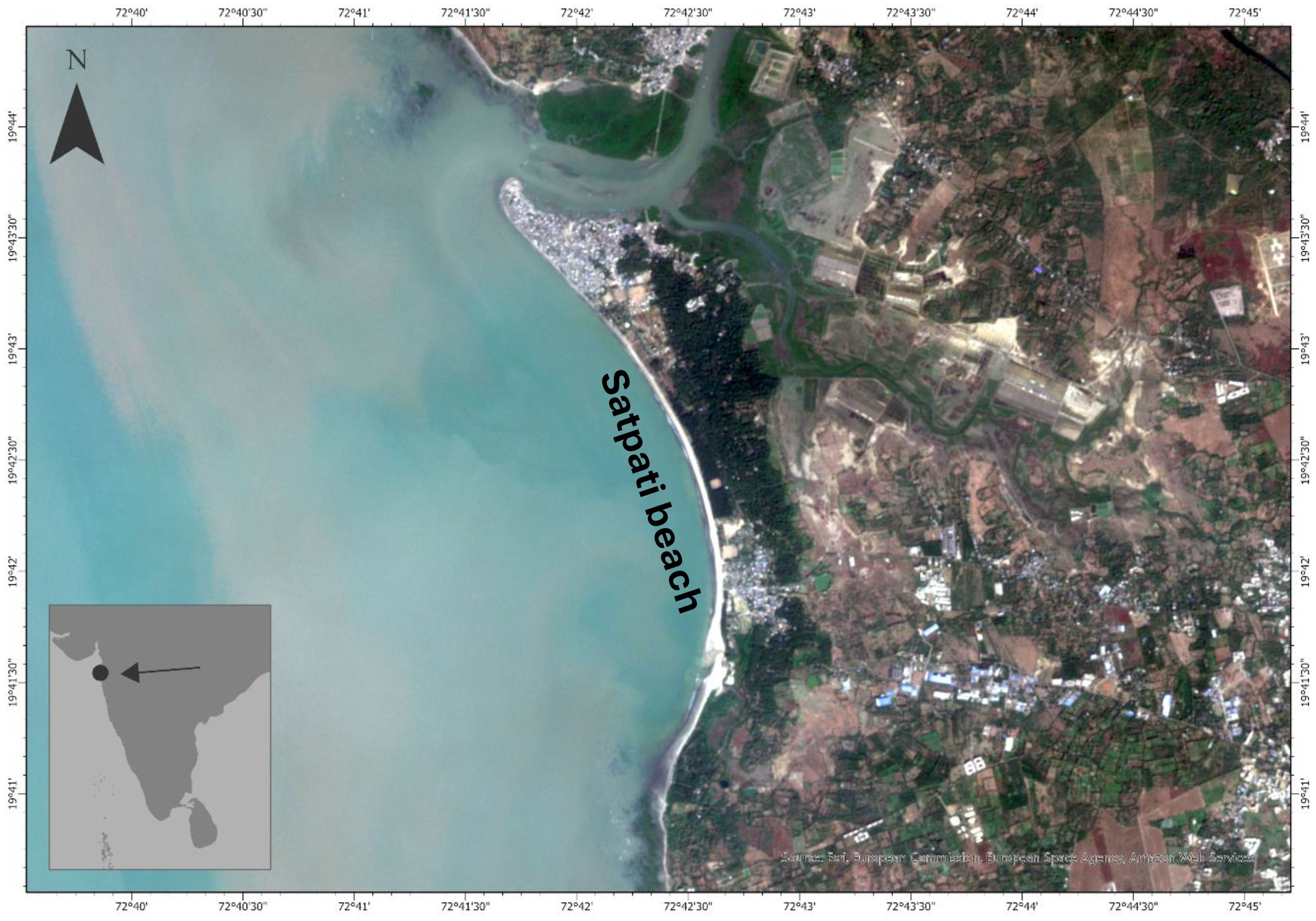
In this study, we focus on developing a multi-database hybrid model to accurately predict the shifts in local shorelines by conducting various field surveys and using field data to improve model simulations. The open sandy beach of Satpati was selected as the study site. The area is located in Palghar District of Maharashtra (Figure 1). The population of Satpati primarily constitutes fisherfolk (approximately 6,500 of the total village population of ca. 17,000, according to 2011 census data), with a major floating tourist population. The village is just south of the Banganga river mouth, with strong tidal currents and sediment movement in the creek region. In the past, ad hoc measures (such as construction of sea walls) were taken to arrest coastal erosion, but the entire length of open sea beach was left unprotected and unmanaged. The sea wall has been eroded by strong wave action and multiple cyclones (some of severe category [tropical cyclone with a wind speed of 64–85 knots (74–98 mph; 119–157 km/h) or higher], see Figure 2) and there has been severe coastal erosion during the past 5 years. In this study, we have selected a 5-year time frame (2019–2023) starting from our first data collection campaign at the site.

Figure 1

Figure 1. Location map of Satpati beach, Palghar, Maharashtra.

Figure 2

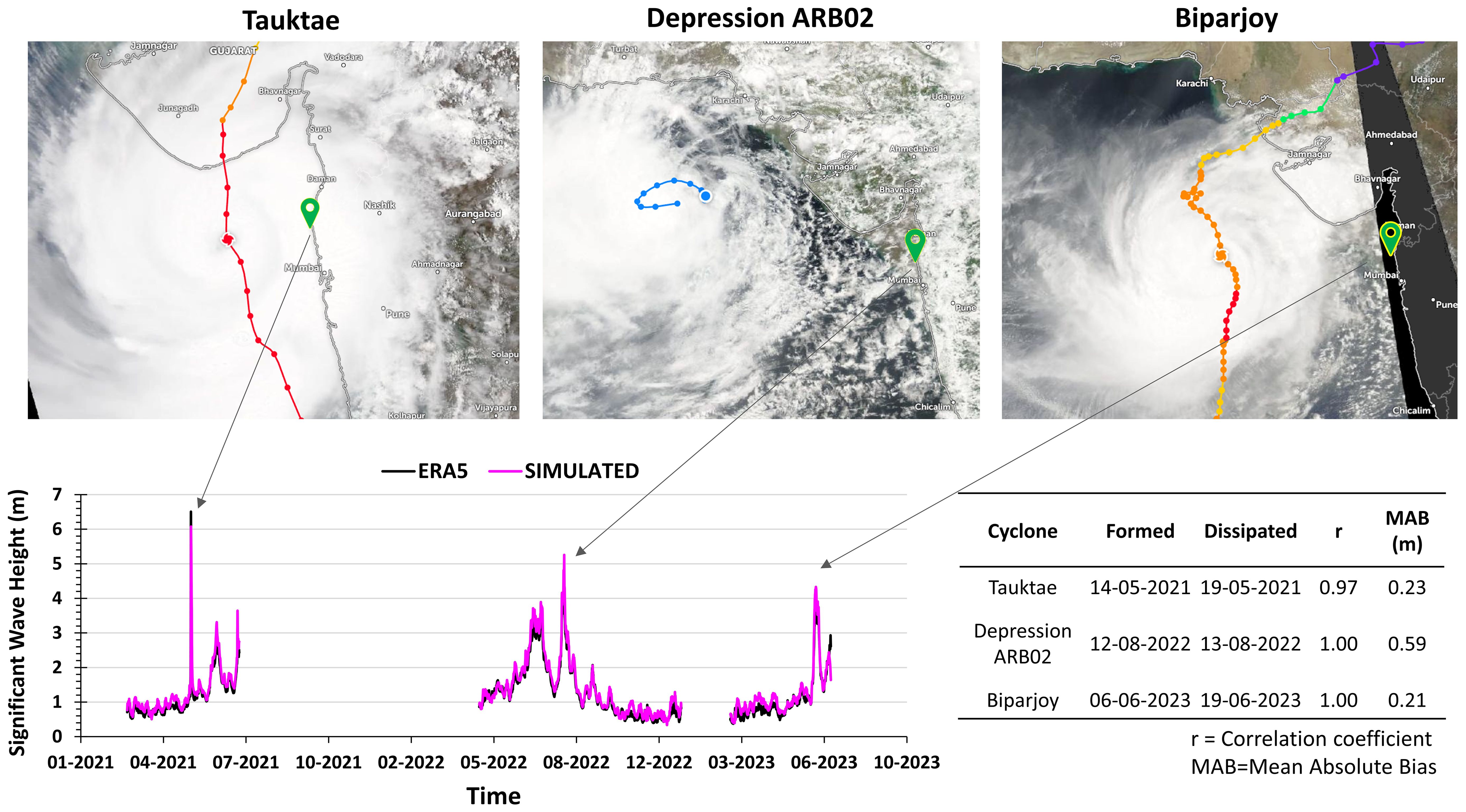
Figure 2. Tracks of cyclones Tauktae and Biparjoy (red markers) and a major depression ARB02 (blue markers) off the study area. The time series plot of extreme high waves (black line: ERA5 and pink line: simulated using numerical spectral wave model) during the abovementioned cyclone period (72.5°E, 19.5°N) off Satpati.

3 Data and methods

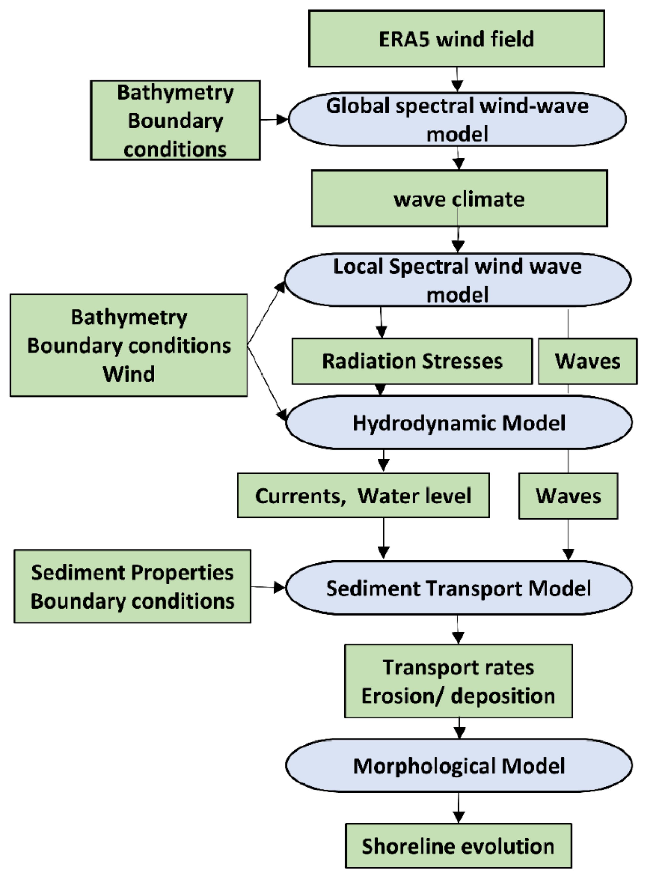
This section gives a brief overview of data collection methods and datasets used for mathematical modeling of hydrodynamic and morphodynamic aspects of the study. A flowchart of the methodology is provided in Figure 3, Table 1 summarizes the data used in model calibration and prediction.

Figure 3

Figure 3. Methodology flowchart.

Table 1

Table 1. Data for model development.

A summary of the methodology flowchart is given below:

1. Data collection and preprocessing

   ERA5 wind data were gathered from the open-source repository of European Centre for Medium-Range Weather Forecasts (ECMWF ERA5). Historical shoreline positions, bathymetry, and sediment data were obtained from toposheets and field surveys. All the datasets were then pre-processed to ensure compatibility and quality, including georeferencing and interpolation.

2. Hydrodynamic and wave modeling

   Coastal hydrodynamics at the study site was simulated using the MIKE 21 numerical model to calculate wave conditions, currents, and water levels. We then nested the regional model to a more focused local model and incorporated the wave transformation processes, including refraction, diffraction, and shoaling, to accurately represent wave propagation along the shoreline.

3. Sediment transport modeling

   The MIKE 21 sediment transport model was used to simulate the movement of sediment along and across the shoreline. Important transport mechanisms were included in the modeling, like the longshore and cross-shore sediment transports, bedload, and suspended load transport.

4. Shoreline evolution modeling

   The outcomes of the hydrodynamic and sediment transport models were integrated to predict shoreline evolution over time. In addition, in this study, we calculated the depth of closure separately for the six identified transects such that the coastal profile predictions would be more realistic and accurate. These values were then fed back into the shoreline evolution model to modify the calculations for a better and accurate representation of the coastal profile over time.

5. Model calibration and validation

   All our model parameters were calibrated using historical and field data and observed coastal changes. Datasets used for model calibration and validation are listed in Table 1.

3.1 Sediment data

The sediment samples were collected along the Satpati beach during the survey. The sediments were tested at the geotechnical laboratory of the Department of Civil Engineering, Indian Institute of Technology Bombay. Standard procedure was followed in carrying out all the tests (following Anderson, 2007). Sieve analysis was carried out, and it was observed that the d₅₀ value pertaining to the site varied between 0.08 and 0.38 mm. The coarser sediments (d₅₀ = 0.38 mm) were found near the dune and fine sediments with an average d₅₀ of 0.1 mm were consistent along the swash zone.

3.2 Bathymetry and topography survey

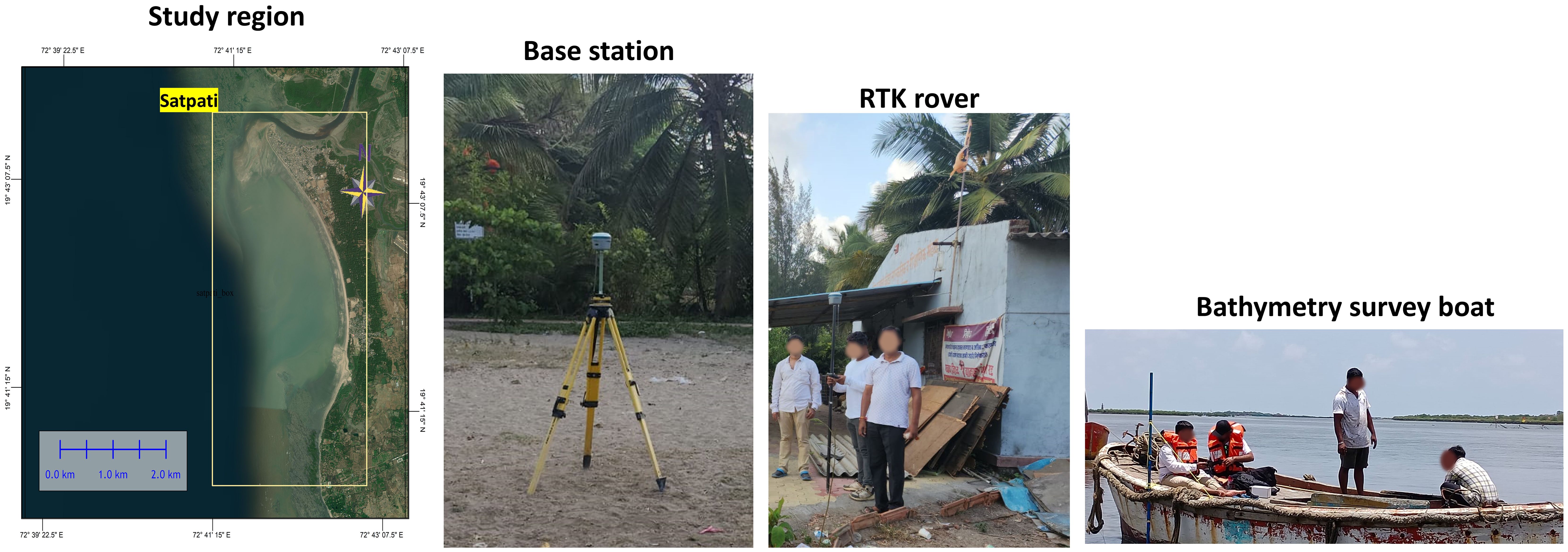
The bathymetry survey was carried out using an echosounder mounted on a fishing boat, and topography survey was performed with the Real-Time Kinematic Differential Global Positioning System (RTK DGPS). The nearshore bathymetry and topography survey outputs were merged with Satpati toposheet to obtain the high-resolution nearshore bathymetry and topography. This dataset is used for regional-scale hydrodynamic studies. The General Bathymetric Chart of the Oceans (GEBCO) datasets were used for offshore global wave modeling. All the datasets are merged with reference to the chart datum. Figure 4 shows the field data setup and visit by staff.

Figure 4

Figure 4. Field survey zone map and equipment used for survey.

3.3 Tidal levels

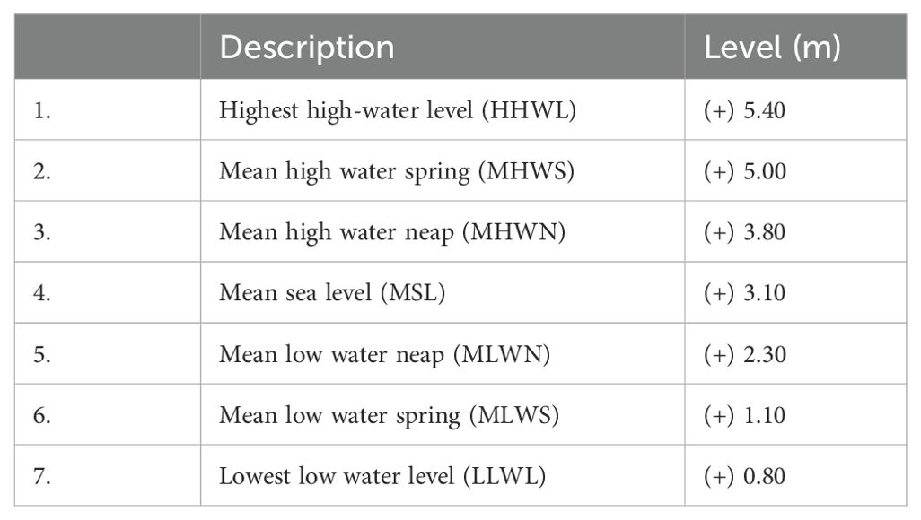
Satpati experiences semidiurnal macrotides, with a tidal range of 4.6 m varying between 0.8 and 5.4 m. The tidal level with reference to chart datum is given in Table 2. The tidal levels are taken from the hydrographic chart published by the Maharashtra Maritime Board. The measured tidal level time series during cyclone Phyan reported by Vinod Kumar et al. (2012) is used for validation of the hydrodynamic model.

Table 2

Table 2. Tidal levels at Satpati.

3.4 Hydro-morphodynamic modeling

Climate change drives potential changes to wave climate (Hemer et al., 2013; Erikson et al., 2015; Shope et al., 2016), which must be accounted for when predicting long-term coastal evolution or determining design of coastal structures. Accurate predictions of nearshore wave conditions are needed because the formulations for shoreline change and longshore sediment transport are highly sensitive to wave conditions. Variations in wave angle and wave energy can significantly affect the calculation of longshore transport and equilibrium shoreline response, respectively. In this study, we used a third-generation spectral wave model MIKE21 (DHI, 2024) to simulate the wave climate over the Indian Ocean region and subsequent smaller domains. MIKE21 is an operational wave simulation model of the Danish Hydraulic Institute and has been extensively validated for wave simulation (Sørensen et al., 2004; Venugopal and Smith, 2007; Remya et al., 2012; Chowdhury and Behera, 2018). The phase-averaged numerical spectral wave model (MIKE21 SW) simulates the growth, decay, and transformation of wind-generated waves and swell from offshore areas by solving the wave action balance equation. The wave climate over the Arabian Sea is dynamic in nature throughout the year due to the southwest monsoon, shamal winds, and swells from the Southern Ocean (Aboobacker et al., 2011; Glejin et al., 2013). Therefore, to properly capture the wave climate at study location, we first developed a global wave model (in this case, for the Indian Ocean domain, left-hand image, Figure 5) and, subsequently, constructed a high-resolution regional wave model (middle image, Figure 5), which was forced with waves extracted from the global model to simulate the nearshore wave climate corresponding to the study area. We used the GEBCO bathymetry data for the global and regional wave models, but to improve predictions near the coast, we added the local bathymetry data obtained from various site visits (right-hand image, Figure 5). We ran the wave model using wind forcing from the European Centre for Medium-Range Weather Forecasts (ECMWF ERA5). The fully spectral formulation with instationary time formulation in MIKE21 SW model is used. The fully spectral formulation considers the complete wave action balance equation without any parameterization, and it results in the capability of the model to represent the complex sea states with multiple peak frequencies. In the fully spectral formulation, the source functions are based on the WAM Cycle 4 formulation (Komen et al., 1994). The wave action balance equation is given below:

Figure 5

Figure 5. Global to local scale wave model domains. Local wave model domain with high-resolution bathymetry obtained during field visits.

$\begin{array}{ll}\frac{dN}{dt}+\nabla .(vN)=\frac{S}{\sigma }& (1)\end{array}$

where N is the wave action density spectrum (N = $\frac{E(\sigma ,\text{θ})}{\sigma }$, E is the wave energy density spectrum); $\sigma$ is the relative angular frequency ($\sigma$ = 2πf); f is the wave frequency; θ is the direction of wave propagation; $v$ is the propagation velocity; S is the energy source function (S = S_in + S_nl + S_ds + S_bot + S_surf); S_in is the wind energy input; S_nl is the energy transfer due to quadruplet wave–wave interaction; S_ds is the dissipation of energy due to white capping; S_bot = dissipation of energy due to bottom friction; and S_surf = dissipation of energy due to depth induced breaking.

The time evolution of the action density wave spectrum over a spatial grid is obtained by solving the wave action balance equation with an implicit, cell-centered finite volume method. The model is based on an unstructured flexible mesh that allows simultaneous computation at regional (coarser) and local (finer) scales, in which time integration is performed using the fractional step approach. The time step is dynamic and estimated based on a constrained Courant–Friedrichs–Lewy (CFL) number of 0.8. The water level variation is not considered for the global wave model, whereas the wave level variation is accounted in regional and local wave models. The generation waves and its growth depend on the energy transfer from wind and wave age; thus, we have used coupled formulation with a Charnock parameter of 0.01 to realistically represent the exchange of energy considering both wind and wave states as per Jassen’s formulations (Komen et al., 1998). The waves can dissipate the energy in deep water through breaking due to higher steepness, known as white capping. The source function for white capping is based on the formulation given by Hasselmann (1974), and this dissipation is controlled through two calibration parameters: Cdis and DELTAdis; Cdis controls the white capping dissipation and DELTAdis controls the dissipation rate. For the current study domain, a Cdis of 2.1 and a DELTAdis of 0.6 are found to be suitable. When waves reach intermediate or shallow waters, the bottom friction and depth-induced breaking control the dissipation of source terms. The bottom friction is specified in the form of Nikuradse roughness (5e-5 is considered for this domain) and a free breaking parameter (ratio of wave height and water depth) of 0.79 is used. The source term for depth-limited wave breaking is based on the formulation by Battjes and Janssen (1978). Overall, the spectral wave model simulates the growth, transformation, and decay of wind-generated waves and swells considering the physical processes of wave generation by wind, dissipation due to bottom friction, deep and shallow water wave breaking, refraction, shoaling, and wave–current interaction. The simulated wave climate is validated with wave parameters provided by observations from buoys located in the Arabian Sea (Figure 6). The global wave model performed well in representing the hindcast daily means of significant wave height (H_s, correlation coefficient of 0.96) and mean wave period (T_m, correlation coefficient of 0.86). The comparison of simulated H_s and T_m with observed AD07 (2014–2016) and nearshore [Karwar (2012–2019), Ratnagiri (2012–2019), and Versova (2016–2019)] buoy measurements are shown in Figures 7, 8, respectively. Furthermore, the model performs well across diverse climate variable scales. Notably, a greater performance of the global wave model is observed in capturing extreme wave climate during cyclonic periods (with a mean correlation coefficient of 0.99 and a mean absolute bias of 0.34 m), as shown in Figure 2; this enhances the reliability of the wave model.

Figure 6

Figure 6. Location of buoys used to validate the wave model.

Figure 7

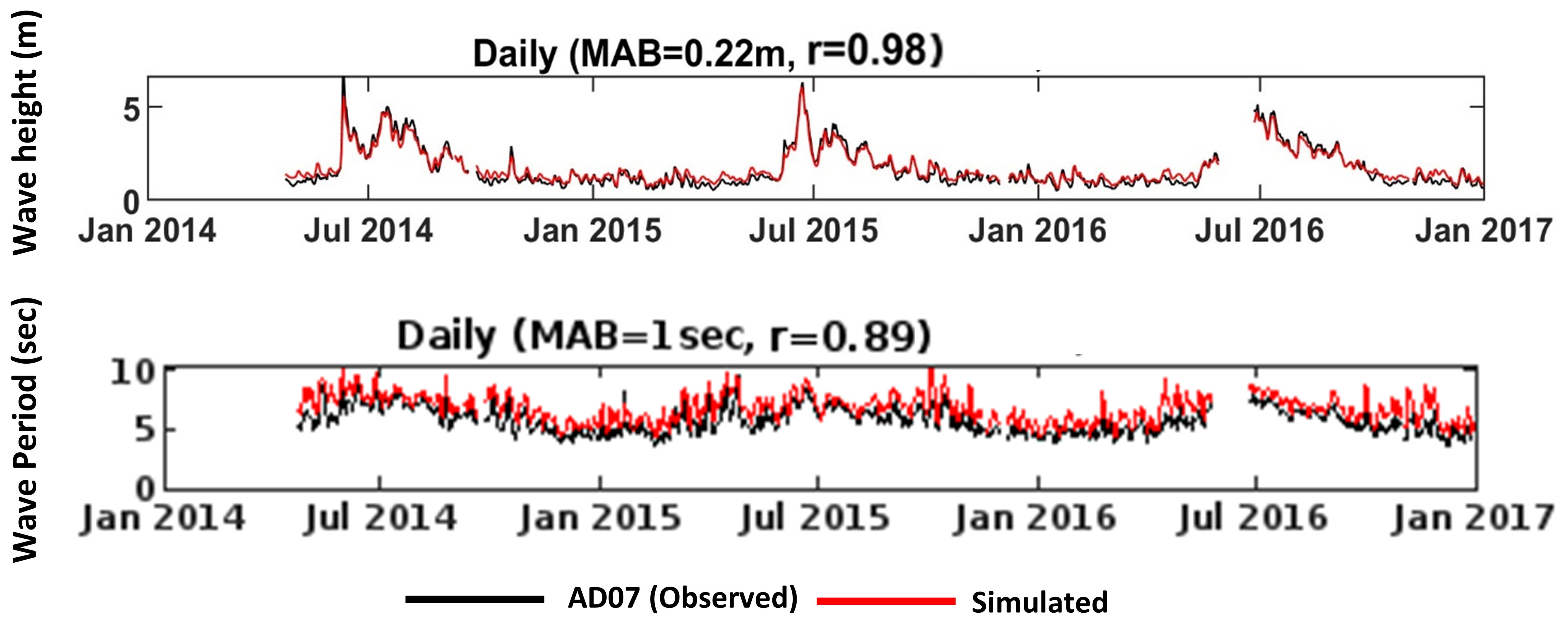
Figure 7. Comparison of simulated wave heights (upper plot)and wave periods (lower plot) with observed values at the AD07 buoy. MAB = Mean Absolute Bias and r = Correlation coefficient.

Figure 8

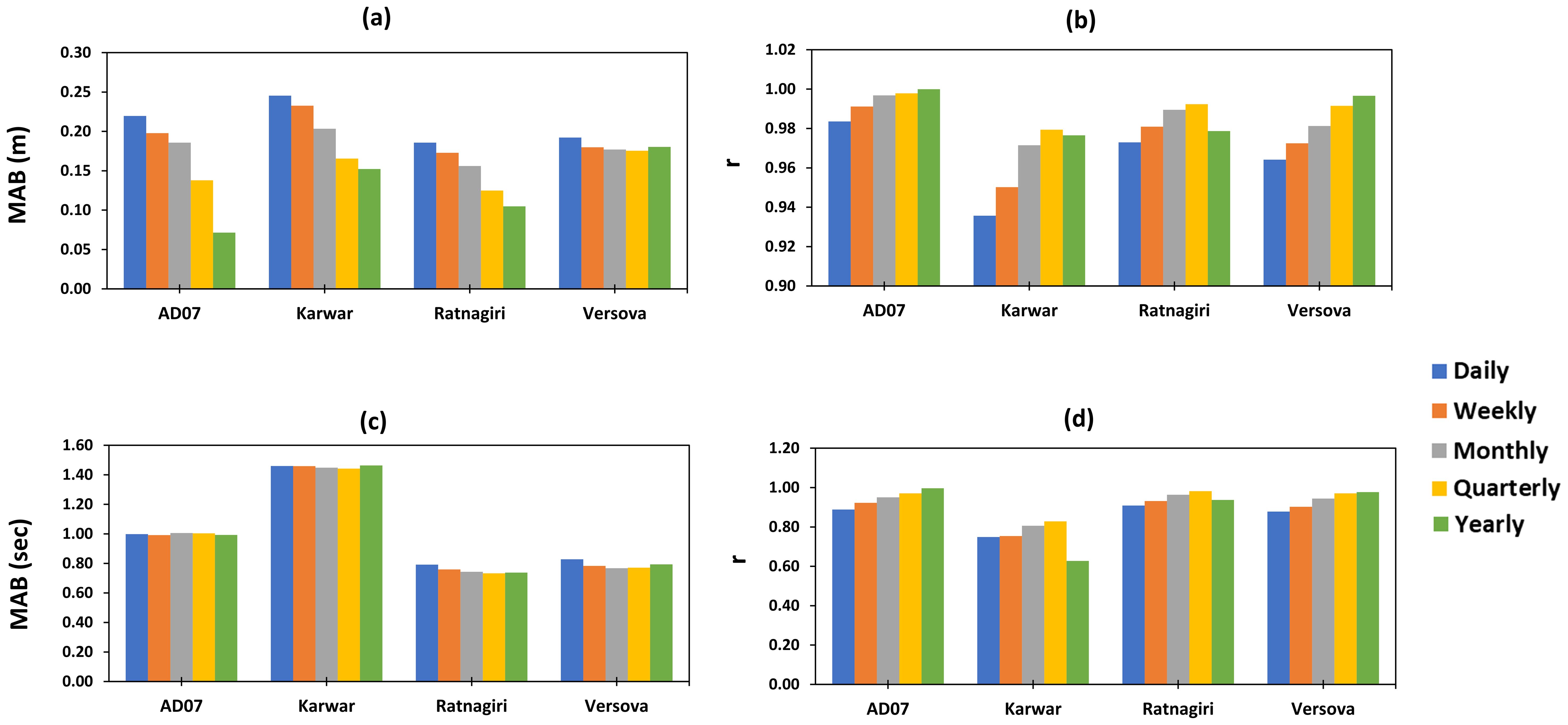
Figure 8. Comparison of simulated wave heights (A, B) and wave periods (C, D) with observed values at the nearshore buoys—Karwar, Ratnagiri, and Versova. MAB = mean absolute bias and r = correlation coefficient.

The coupled wave (MIKE21 SW), hydrodynamic (MIKE21 HD), sediment (MIKE21 ST), and morphology (MIKE21 SM) models are used to investigate the shoreline changes. The wave climate and radiation stresses calculated from the numerical spectral model are given as input to the hydrodynamic model. The depth-integrated incompressible Reynolds averaged Navier-Stokes equations, i.e., shallow water equations, are governing equations, as given below:

$\begin{array}{ll}\frac{\partial h}{\partial t}+\frac{\partial h\overline{u}}{\partial x}+\frac{\partial h\overline{v}}{\partial y}=hS& (2)\end{array}$

$\begin{array}{ll}\begin{array}{l}\frac{\partial h\overline{u}}{\partial t}+\frac{\partial h{\overline{u}}^2}{\partial x}+\frac{\partial h\overline{vu}}{\partial y}\hfill \\ =f\overline{v}h-gh\frac{\partial \eta }{\partial x}-\frac{h}{{\rho }_o}\frac{\partial P_a}{\partial x}-\frac{g{h}^2}{2{\rho }_o}\frac{\partial \rho }{\partial x}+\frac{{\tau }_{sx}}{{\rho }_o}-\frac{{\tau }_{bx}}{{\rho }_o}\hfill \\ -\frac{1}{{\rho }_o}\left(\frac{\partial S_{xx}}{\partial x}+\frac{\partial S_{xy}}{\partial y}\right)+\frac{\partial }{\partial x}(h{T}_{xx})+\frac{\partial }{\partial y}(h{T}_{xy})+h{u}_{s}S\hfill \end{array}& (3)\end{array}$

$\begin{array}{ll}\begin{array}{l}\frac{\partial h\overline{v}}{\partial t}+\frac{\partial h\overline{vu}}{\partial yx}+\frac{\partial h{\overline{v}}^2}{\partial ty}\hfill \\ =f\overline{u}h-gh\frac{\partial \eta }{\partial y}-\frac{h}{{\rho }_o}\frac{\partial P_a}{\partial y}-\frac{g{h}^2}{2{\rho }_o}\frac{\partial \rho }{\partial y}+\frac{{\tau }_{sy}}{{\rho }_o}-\frac{{\tau }_{by}}{{\rho }_o}\hfill \\ -\frac{1}{{\rho }_o}\left(\frac{\partial S_{yx}}{\partial x}+\frac{\partial S_{yy}}{\partial y}\right)+\frac{\partial }{\partial x}(h{T}_{xy})+\frac{\partial }{\partial y}(h{T}_{yy})+h{v}_{s}S\hfill \end{array}& (4)\end{array}$

where h is the total water depth (h = $\eta$+d), $\eta$ is the surface elevation and d is the still water depth; $\overline{u}$ and $\overline{v}$ are the depth-averaged velocity components in the x and y directions; S is the energy source dissipation term; f is the Coriolis force parameter (f = 2Ωsinø, Ω is the angular velocity and ø is the latitude); g is the acceleration due to gravity; $P_a$ is the pressure due to atmosphere; $\rho and {\rho }_o$ are the density of sea water and reference water; ${\tau }_{sx} \text{and }{\tau }_{sy}$ are the wind stresses in the x and y directions; ${\tau }_{bx}$ and ${\tau }_{by}$ are the bottom stresses in the x and y directions; $S_{xx}$, $S_{xy}$, $S_{yx}$ and $S_{yy}$ are the component of radiation stress tensor; $T_{xx}$, $T_{xy}$, $T_{yx}$ and $T_{yy}$ are the lateral stresses; S is the magnitude of the discharge due to point sources and its velocity denoted by $u_s$ and $v_s$.

These equations’ spatial discretization is carried out using the cell-centered finite volume method, and an explicit scheme is used for time integration. The hydrodynamic model can estimate the flow parameters considering both tide and wave variations. The influence of tide is accounted for by forcing tide from open boundaries of domain as time series of water level. The radiation stresses from the wave model are accounted for in momentum equations. The eddy viscosity concept is used to model the unresolved small-scale turbulence processes using sub-grid scale models (Smagorinsky, 1963). The Eddy viscosity (Smagorinsky formulation coefficient) of 0.28 is considered. The spatially varying bed resistance (with Manning number 5 m^1/3/s over the reef zones and 32 m^1/3/s over remaining domain) is found from calibration runs. Considering the aforementioned forcings with calibration parameters, the hydrodynamic model estimates the depth-averaged velocity, tidal water levels, wave set-up, and wave set-down by solving the governing equations. The water levels from the hydrodynamic model are validated with the measured water level reported by Vinod Kumar et al. (2012) during the Phyan cyclone. They carried out the water level measurements at a depth of ~15 m off Satpati (72.618075°E, 19.733525°N) using sea level gauge. The current hydrodynamic model shows greater agreement (r = 0.97, MAB = 0.22 m) with the measured water level and showed better performance than Vinod Kumar et al. (2012) model output (Figure 9). The calculated wave and current parameters from the hydrodynamic model, along with sediment properties (d₅₀ = 0.1 mm, sediment grading coefficient of 1.5, relative density of 2.65, and porosity of 0.4), are given as input to the sediment transport model to calculate the sediment transport rates by interpolation from pre-simulated sediment transport table. This table is generated from the quasi three-dimensional sediment transport model in the MIKE21 toolbox, which estimates the vertical variation of time-dependent flow velocity, turbulence, shear stress, and sediment concentration using an integrated momentum approach (Fredsøe, 1984). The sediment transport model estimates the bed load and suspended load based on the formulation of the Engelund and Fredsoe (1976) model. The variation of suspended concentration across the depth is estimated by solving the vertical sediment diffusion equation (Fredsøe et al., 1985), as given below.

Figure 9

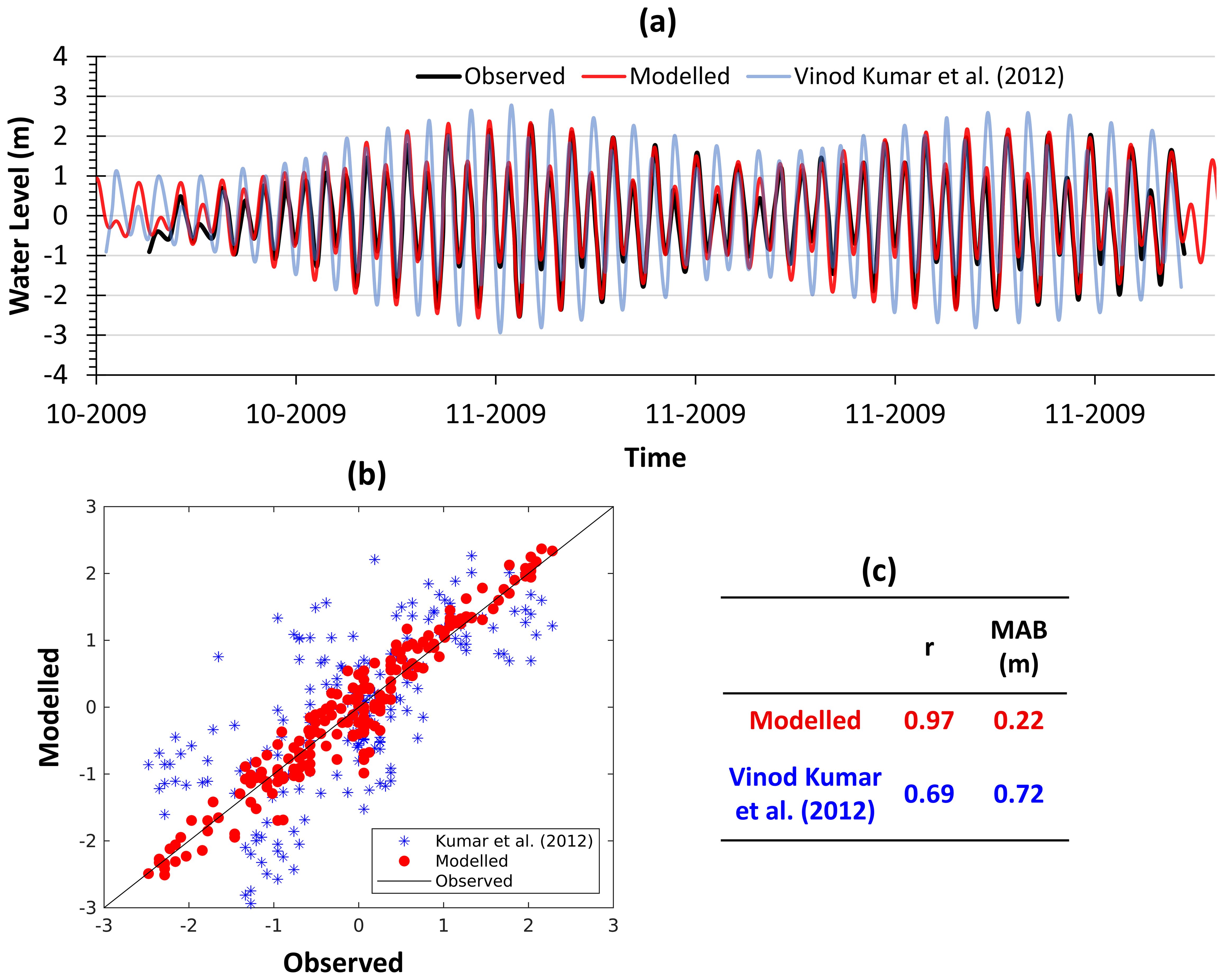
Figure 9. The comparison of modeled water levels relative to observed water levels off Satpati (72.618075°E, 19.733525°N). (A) Time series plot of observed water levels (black line), modeled water level (red line), and the water levels reported by Vinod Kumar et al. (2012). (B) Scatter plot between observed and modeled water levels. (C) Comparison statistics summary; r = correlation coefficient and MAB = mean absolute bias.

$\begin{array}{ll}\frac{\partial c}{\partial t}+\frac{\partial (uc)}{\partial x}+\frac{\partial (vc)}{\partial y}+\frac{\partial (wc)}{\partial z}=\frac{\partial }{\partial x}\left({ϵ}_x\frac{\partial c}{\partial x}\right)+\frac{\partial }{\partial y}\left({ϵ}_y\frac{\partial c}{\partial y}\right)+\frac{\partial }{\partial z}\left({ϵ}_z\frac{\partial c}{\partial z}\right)+w_s\frac{\partial c}{\partial z}& (5)\end{array}$

where c is the concentration volume; the left side of equation represents the temporal variation of c, followed by the advection mechanism [transport of c with flow velocities (u, v and w)]. The right side of the equation represents the diffusion [terms with diffusion coefficients (${ϵ}_x,{ϵ}_y and {ϵ}_z$)] and settling mechanism [last term with settling velocity of sediment $(w_s)$].

Having estimated the concentration of sediments, the total sediment load transport is calculated. The two-dimensional sediment transport model updates the changes in bed level using sediment continuity equation, which is given below:

$\begin{array}{ll}-(1-n)\frac{\partial z}{\partial t}=\frac{\partial S_x}{\partial x}+\frac{\partial S_y}{\partial y}-\Delta S& (6)\end{array}$

where the left side represents the rate of change in bed level (z), and n is the porosity; the right side represents the spatial changes in total sediment transport including provision for beach nourishment (source) or sink rate. Once the rate of bed level change is estimated, the new bed levels are updated at every time step with a forward in time difference scheme (Equation 7).

$\begin{array}{ll}{Z}_{new}=Z_{old}+\frac{1}{1-n}\frac{\partial z}{\partial t}\Delta t& (7)\end{array}$

The two-dimensional sediment transport model results are found to be satisfactory for analyzing shorter timescale changes. However, in applications of investigating long-term morphological changes, the model was found to result in the degeneration of profile due to higher cross-shore transport (Kristensen et al., 2013). This led to the development of the hybrid shoreline morphology model, in which the hydrodynamics and sediment transport rates are calculated based on two-dimensional models, and an update of morphology and shoreline is based on the concept of the one-line model. In the shoreline morphology model, the active nearshore zone is divided into shore normal strips, the offshore extent of these strips should cross the depth of closure, and the cross-shore bed variation is defined by profile on each shoreface strip. For each time step, the one-line shoreline model integrates the total sediment volume changes along the shoreface strip and updates the change in shoreline position by solving a one-line equation (Kaergaard and Fredsoe, 2013). In this study, the shoreline model is forced with a single projected time series of wave conditions (Hegermiller et al., 2016) as we are interested in past shoreline evolution. This single source time series type wave forcing scenario represents only one instance of representing the wave climate and subsequent coastal evolution. When predicting future shoreline shifts, the range of potential shoreline positions can be improved by using an ensemble wave forcing approach providing estimates of uncertainty; however, this comes at a significantly increased computational effort (by a factor representing the number of ensemble wave scenarios).

3.5 Shoreline change prediction

3.5.1 Importance of local depth of closure in shoreline change prediction

The depth at which significant sediment motion is absent is often called the depth of closure (hereafter, Dc). It is time-dependent: the longer the wave period being considered, the larger the Dc value (Stive et al., 1992). Kraus et al. (1999) highlighted temporal significance when they proposed that, for a given time interval, Dc should be defined as the depth seaward where neither a significant change in bottom elevation nor a significant net sediment exchange between nearshore and offshore occurred. Dc can be estimated using a range of techniques, including grain-size trends (Larson, 1991; Work and Dean, 1991) and orientation of offshore contours and wave statistics (Hallermeier, 1981). It can be defined as the ratio of change in cross-sectional area divided by the advance or retreat of the high-water line, or other convenient contours that can be determined from an analysis of beach profiles, providing they continue far enough underwater (Simm, 1996). Field surveys consist of repeated profile measurements over multiple years to establish the depth at which the seabed remains stable (Nicholls et al., 1996). The estimated Dc through the profile survey method is accurate but requires long-term profile time series data. In the absence of field measurements, the mathematical formulas proposed by Hallermeier (1979) and Houston (1996) are recommended.

Hallermeier (1979) proposed an analytical solution for estimating annual Dc using linear wave theory. The Dc formulation is a function of wave height and wave steepness:

$$D_c=2.28H_e-68.5(\frac{H_e^2}{g{T}_e^2})$$

where $H_e$ is the wave height exceeding 12 h per year, g is the acceleration due to gravity, and $T_e$ is the associated wave period.

The existing mathematical formulations are based on specific events ($H_e$) and they do not account for the local sediment characteristics. A newer approach proposed by Aragonés et al. (2018) estimates Dc based on the distribution of cross-shore median sediment size only, but identifying the point of change in sediment size through sampling is complex and costly.

Most Dc studies have focused only on a single transect profile because repeated profile data are not generally available, and these studies mainly use hindcast wave outputs from a single source with coarse resolution bathymetry. This study is an improvement over the existing approach as we not only used transect profiles surveyed in 2019 and again in 2023, but we also improved the wave hindcast during this time period by incorporating higher-resolution nearshore bathymetry (see Figure 5). Here, Dc is estimated through numerical modeling, which accounts both wave hydrodynamics and sediment characteristics along the profile. The following steps were followed:

● An initial average Dc over the domain was calculated based on existing formulas proposed by Hallermeier (1979).

● Profiles were surveyed and constructed from the shoreline to this Dc.

● Wave-driven current and littoral drift along the profile were estimated by forcing with a nearshore significant wave height exceeding 12 h per year and the respective wave period.

● Finally, various points (P1 to P3, Figure 10) were identified, across which the respective depths were identified and beyond which the littoral drift would become zero for each profile, hence giving us actual Dc. The Dc values were estimated using the 12-h exceedance wave data during the same period as the profile measurements for determining the initial Dc as shown in Table 3.

Table 3

Table 3. Analytical estimation of depth of closure (Dc).

Three profiles were constructed to the offshore depth 12 m from shore, as shown in Figure 10. The profiles were forced with wave climate obtained as per Hallermeier (1979). The LITDRIFT module of LITPACK is used to estimate the cross-shore distribution of wave height, current, and littoral drift. The hydrodynamic model of LITDRIFT transforms the wave climate from deep water to each grid point of the profile, and the resolution of the profile reflects the accuracy of processes. The wave processes, such as refraction, are based on Snell’s law, shoaling is estimated by the conservation of wave energy flux, the ratio of wave height to water depth governs the breaking, the wave set-up and set-down are estimated based on the cross-shore gradient in cross-shore radiation stresses, and longshore currents are estimated based on the cross-shore gradient in longshore radiation stress. All these major wave processes and wave-driven currents are clearly reflected in Figure 10 along the profile. The sediment transport might occur in two modes: the first mode is the transport of bed material by sliding, rolling, or jumping within a thin layer (~2 * d₅₀ thickness) near the bed, and in the second mode, the suspended sediments transport along the predominant current direction. Along the profile, the uniform mean grain size of 0.1 mm is considered and the respective fall velocity and bed roughness (2 * d₅₀) are estimated, and given as input to model. The LITPACK estimates the bed load transport based on the instantaneous Shields parameter and the suspended load by integrating the product of sediment concentration and mean circulation current over the wave period. The concentration of suspended sediment varies over time and water depth, and it is estimated by solving a diffusion equation (one-dimensional form of Equation 5) using the finite difference technique. The mean circulation currents are obtained from the hydrodynamic model. The total sediment transport (sum of bed load transport and suspended load transport) is computed at the grid point of the profile, and the net sediment transport across the profile is shown in Figure 10C. The predominant transport is observed in breaking zones. The LITPACK modeling suite has been applied successfully by many investigators for the Indian coast (for example, Noujas and Kankara, 2018; Rao et al., 2009). The mean size of the sediment used was 0.1 mm, as obtained from the sample collected during field visits. The cross-shore distribution of wave height, current, and net sediment transport along the profiles (Figures 10B, C) was analyzed, and the depth beyond which current and littoral drift becomes almost zero was identified as the working Dc (Figure 10). We found that Dc obtained as per the Hallermeier (1979) equation was underestimated when compared to the outcomes of the deterministic model run for the same wave parameters, implying that accurate wave hydrodynamics and sediment properties along the transects are important for Dc calculations. The offshore extent of the local domain was considered beyond the mark of working Dc and the coastal profile in the shoreline morphology model was also considered. The summary of conventional and new methodology approaches are shown in Figure 11.

Figure 10

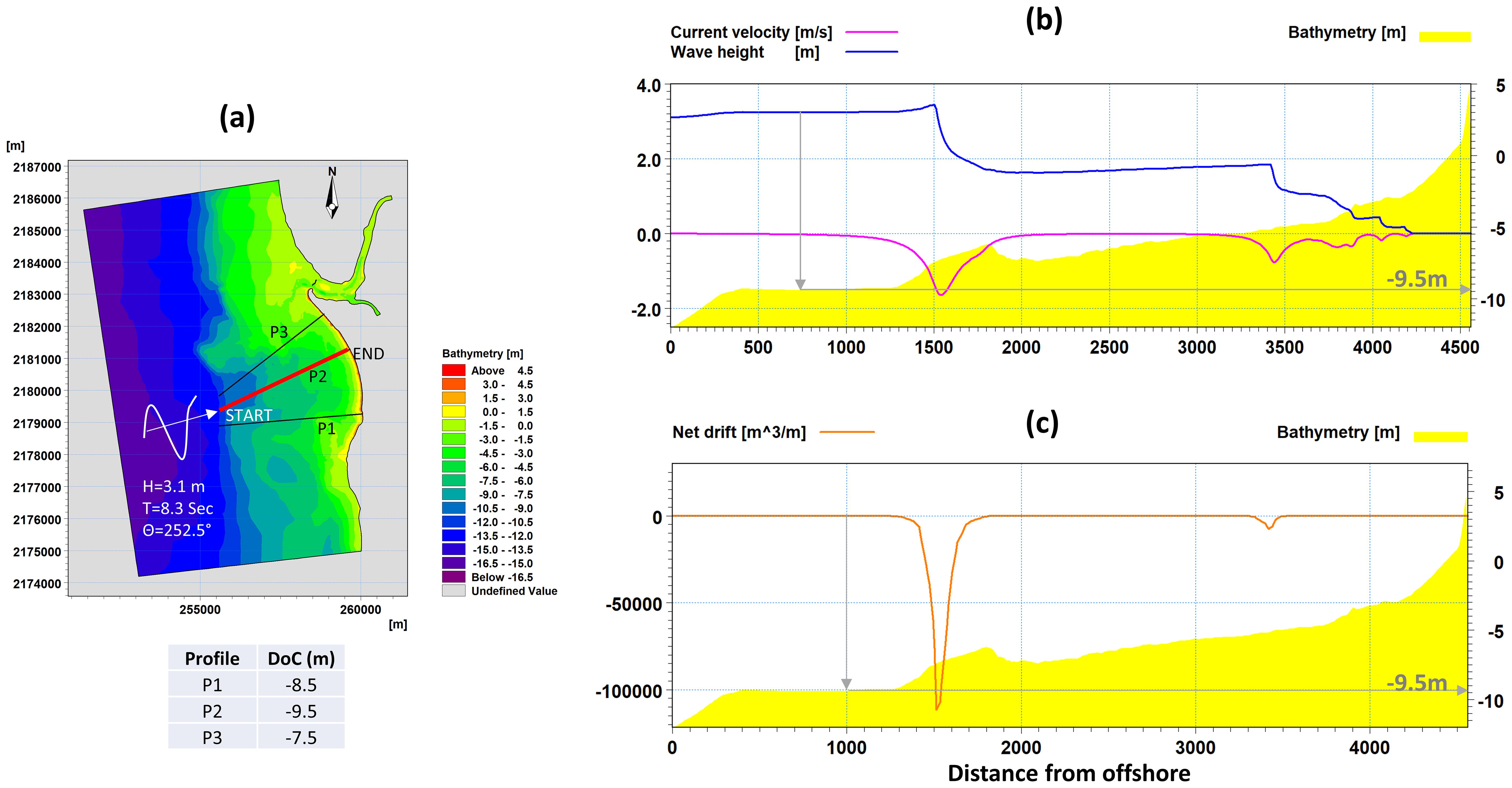
Figure 10. (A) The spatial extent of the study domain showing profiles used for estimating depth of closure. (B) Variation of wave height and current along profile P2. (C) The net littoral drift along profile P2.

Figure 11

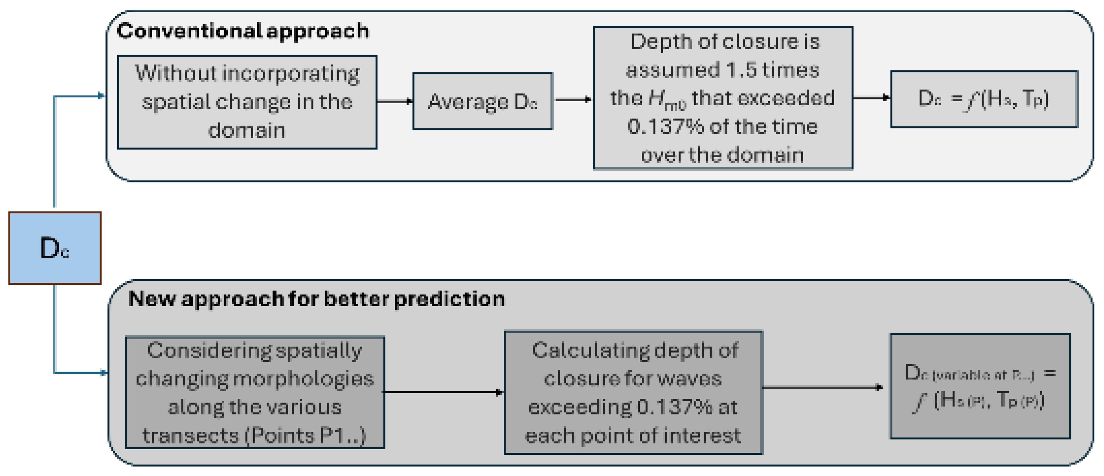
Figure 11. New approach proposed in this study for accurate shoreline prediction by incorporating local Dc in the shoreline models.

4 Results and discussion

4.1 Wave climate at the study area

The Indian Ocean region may be subdivided into two main water bodies, the northern Indian Ocean region and the southern Indian Ocean region, based on its spread over both hemispheres. Furthermore, the Indian subcontinent divides the northern Indian Ocean into the Arabian Sea on the west and the Bay of Bengal on the east. The ocean–land interaction that exists in the northern Indian Ocean due to the presence of the Indian subcontinent influences the wave climate in this region. The Indian subcontinent experiences southwest monsoon from June to September (JJAS) and northeast monsoon from October to December (OND). Most of the wave activity in the AS is driven by the monsoon winds (Chowdhury and Behera, 2019; Chowdhury et al., 2019). The current study region, along the west coast of India, is a stretch of open sandy beach facing the Arabian Sea where the predominant waves are observed from south-westerly and westerly directions. The typical annual and seasonal wave climate near the area of interest is shown in Figure 12. Here, interest is in the microscale; hence, the results were extracted at various locations along the beach at approximately 1-km (or lesser) intervals across the beach into deep water at 4–5 km apart. Table 4 shows the external forcings associated with the shoreline evolution of a beach considered at the microscale.

Figure 12

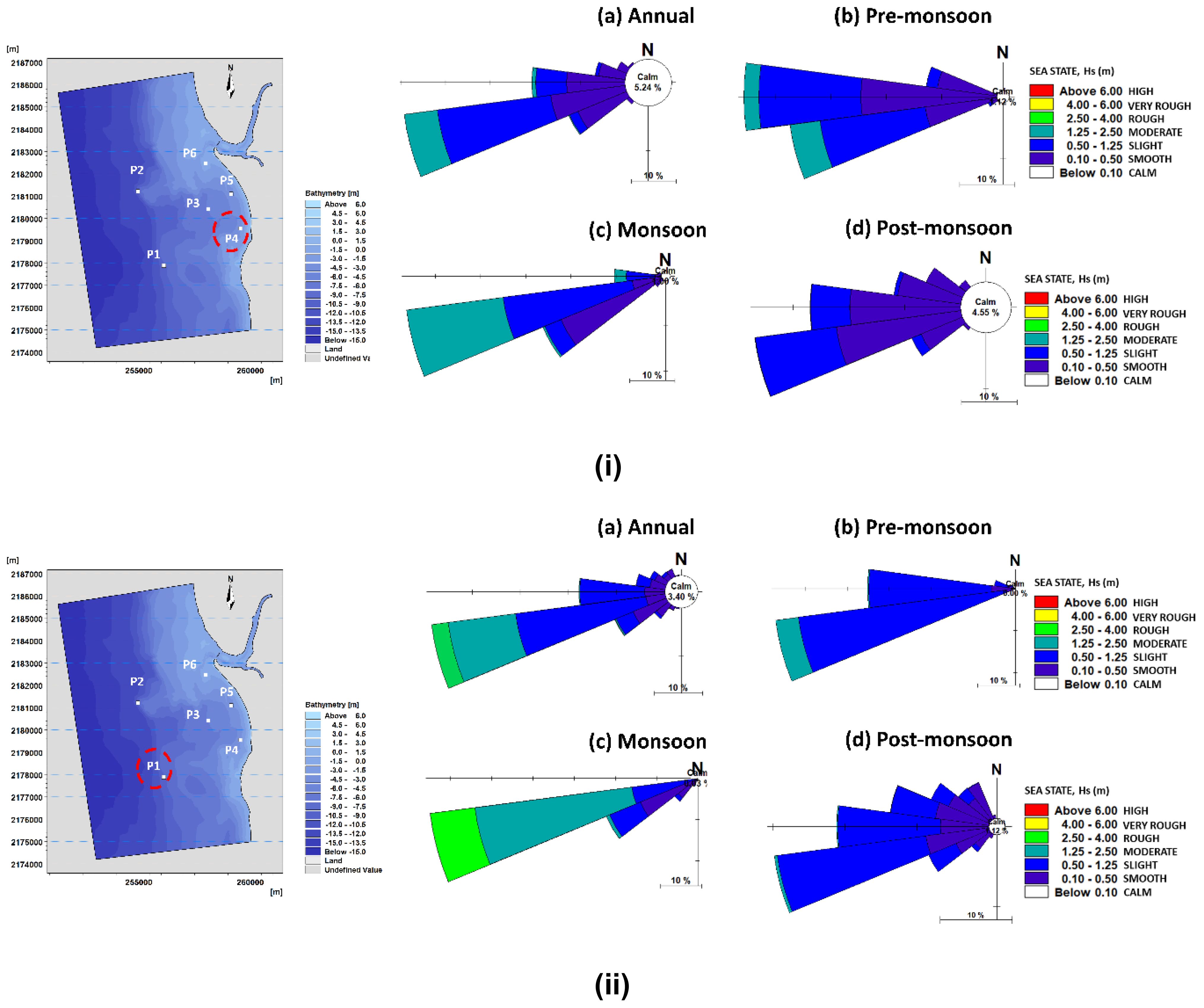
Figure 12. Typical wave climate at two points (i) close to the shore (left-hand image, upper panel) and (ii) in deep water (left-hand image, lower panel), over annual and seasonal scales (pre-monsoon, monsoon, and post-monsoon), averaged over 2019–2023. Hs = Significant wave height.

Table 4

Table 4. External forcing associated with microscale evolution of shorelines.

4.2 Shoreline shift calculations

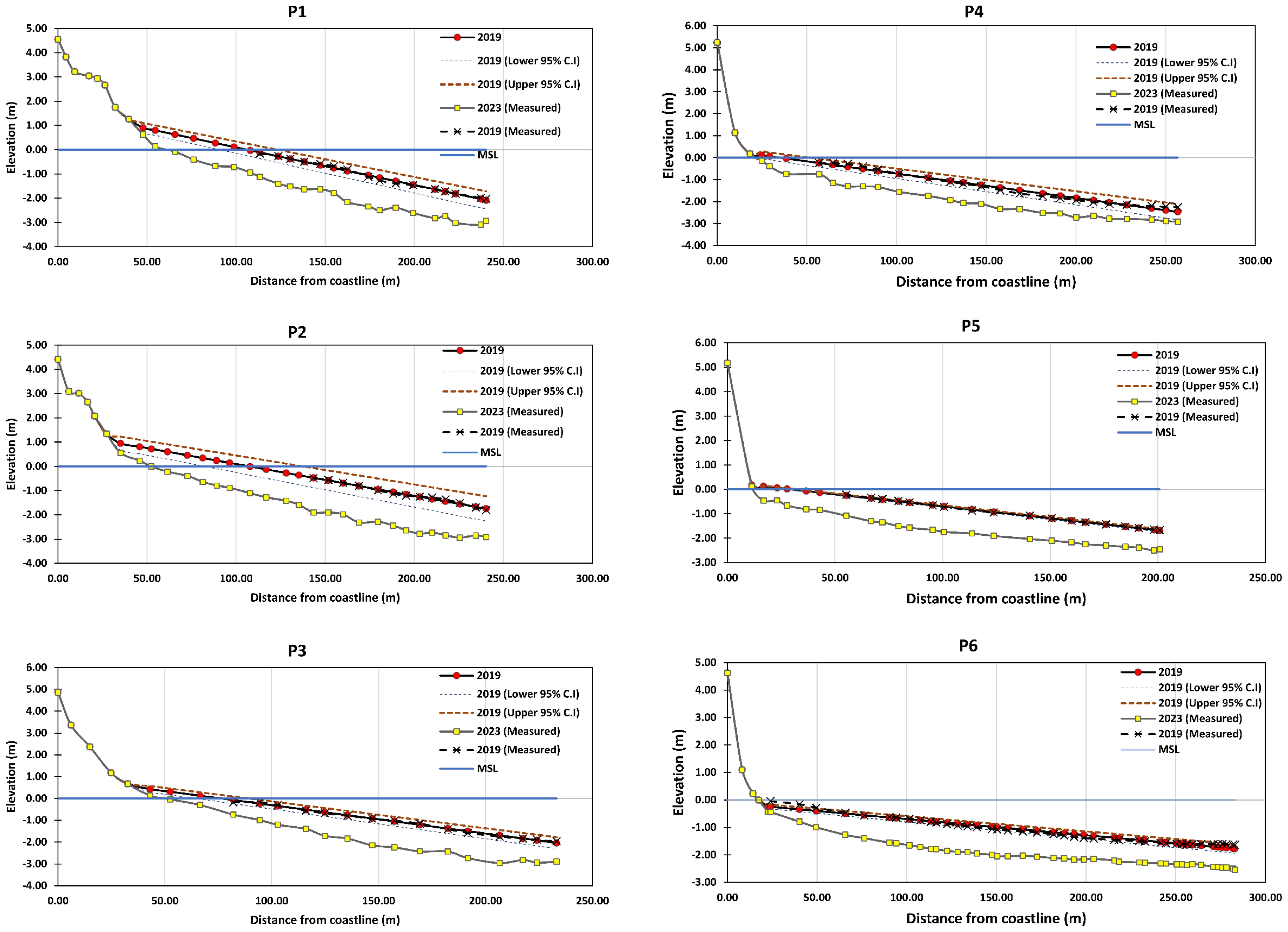
Shoreline change analysis and prediction are important for integrated coastal zone management. The shifts in shorelines are conventionally estimated using data from field and/or aerial surveys, numerical models, and satellite remote sensing images. The Satpati coastline is macrotidal and comprises a wave-dominated sandy beach with an average length of 5.5 km. The RTK-GPS survey was carried out on 12 June 2023. An element of the survey involved measuring six cross-shore profiles, hereafter referred to as P1, P2, P3, P4, P5, and P6 (Figure 13).

Figure 13

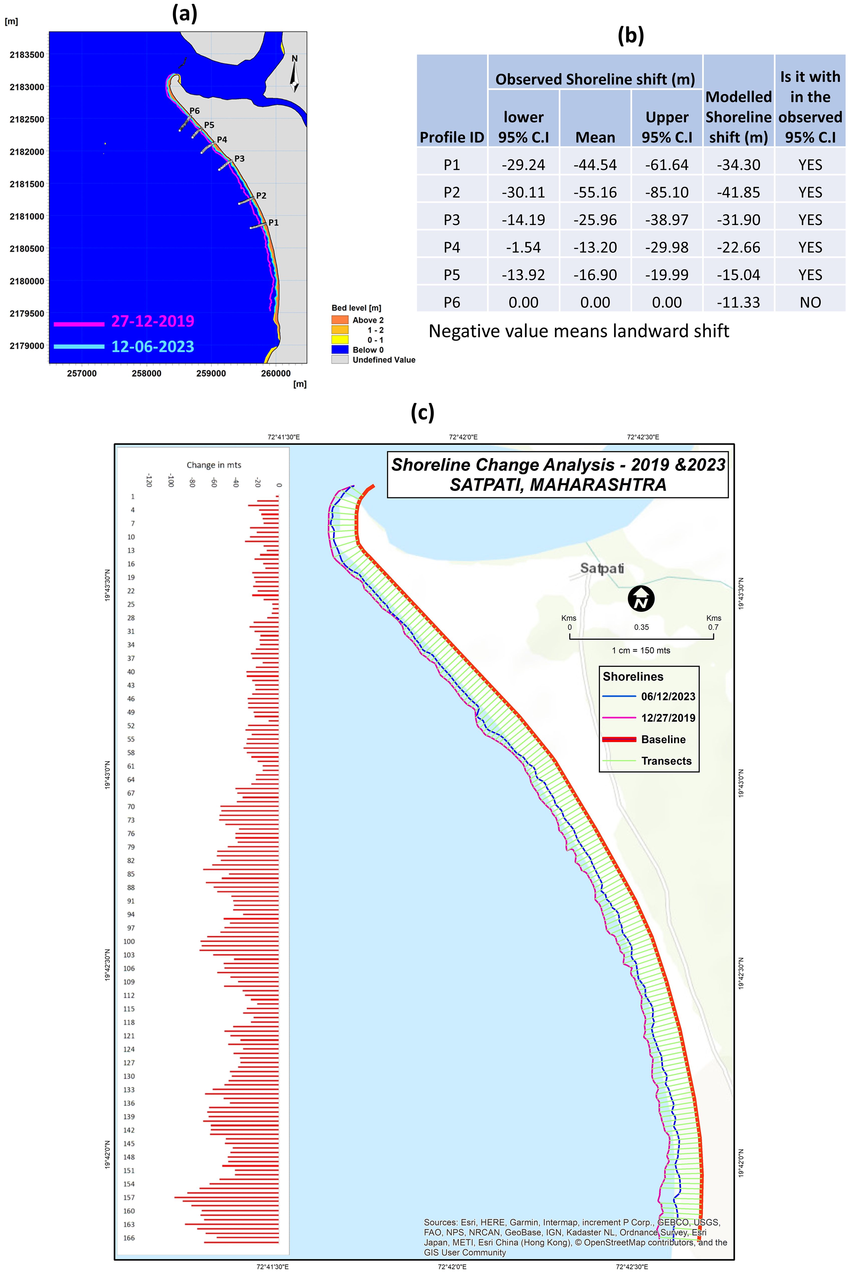
Figure 13. Shoreline shift between 2019 and 2023 based on hydrographic and MSL chart data (2019) and field measurements (2023). (A) shows the Transect Points (P1–P6); (B) shows the uncertainty range for the predicted 2019 shoreline; and (C) shows the landward shift in the 2023 shoreline compared to the shoreline in the year 2019.

In general, the shoreline is defined as a position at which the highest high tide line intersects the beach profile. For the current study region, no significant change in the shoreline position (based on high tide line) is observed during the study period. However, a significant rate of erosion is observed along all profiles located in the swash zone (tidal variation zone), which has led to the landward shift in the point of intersection (i.e., MSL line and beach profile). Thus, the position at which the MSL intersects the beach profile is defined as shoreline for the purpose of the current study.

The historical cross-shore profiles (27-12-2019) were extracted from the hydrographic chart (dashed line with markers in Figure 14). The coastal profiles extracted from the 2019 hydrographic chart was present close to mean sea level (MSL) but did not touch the actual MSL line (dotted blue line in Figure 14). Therefore, the profiles were extended using the linear regression technique to make them coincide with the MSL. Linear regression for shoreline changes prediction involves using a mathematical model to analyze the relationship between predictor variables (such as coastal features, wave characteristics, sediment transport, etc.) and the response variable, which is typically the change in shoreline position over time. However, owing to the lack of measured data points until the MSL mark, we also estimated the uncertainty range showing three possible 2019 profiles (the regression line and its upper and lower confidence bands) to estimate the shoreline position. In this, we assume the distance from the coastline as the dependent variable and elevation as the independent variable. The goodness of fit of regression line is summarized by R², standard error (SE), and p-value statistics (Table 5). The evolution of cross-shore profiles P1 to P6 between 2019 and 2023 with respect to tides and MSL is shown in Figure 15. For a better understanding of how to read the estimated shoreline and the uncertainty associated with the fitted shoreline, the values estimated at profile P2 are represented in Figure 16, and for all other profiles, the values are listed in Table 5. The position of 2023 shoreline profiles is estimated, and the shoreline shift (i.e., the difference between coastal profiles pertaining to 2019 and 2023) is calculated for P1 to P6. The 2019 shoreline (pink line), 2023 shoreline (cyan line), and a summary of the modeled shoreline shift are summarized in Figure 13. The landward shift of shoreline is observed along the entire Satpati, indicating an active rate of erosion along the beach (Figure 13C). It is observed that the erosion is higher near the southern end of the beach compared to the northern region of the Satpati coast. The shifts in the coastal profiles (estimated using linear regression) from the hydrographic chart baseline is within the confidence interval range for the first five profiles (P1–P5), whereas for profile P6, we observe that the change is negligible, indicating a stable coastal profile. This is attributed to the construction of the sea wall in the northern part of the beach, which might have hindered sediment exchange.

Figure 14

Figure 14. The cross-shore profile at transects P1 to P6.

Table 5

Table 5. The summary statistics of linear regression.

Figure 15

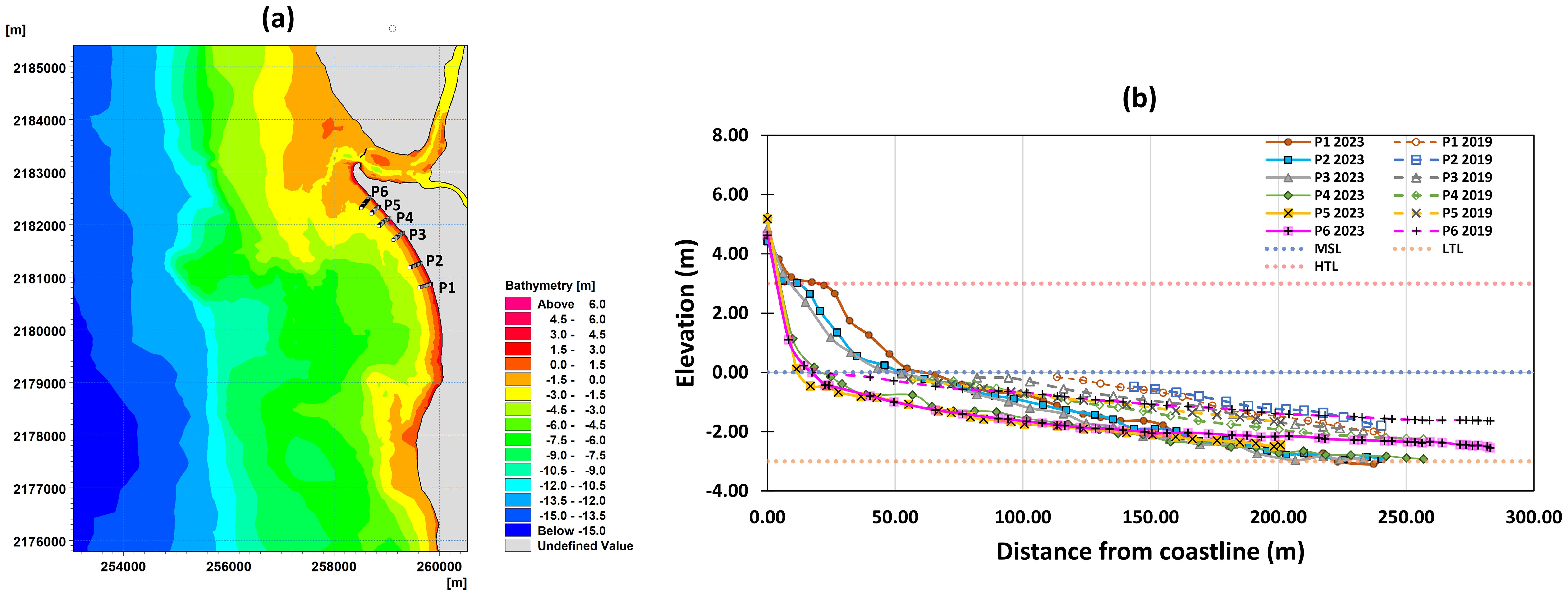
Figure 15. (A) Location of cross-shore profiles and (B) evolution of cross-shore profiles between 2019 and 2023 with respect to tides and MSL.

Figure 16

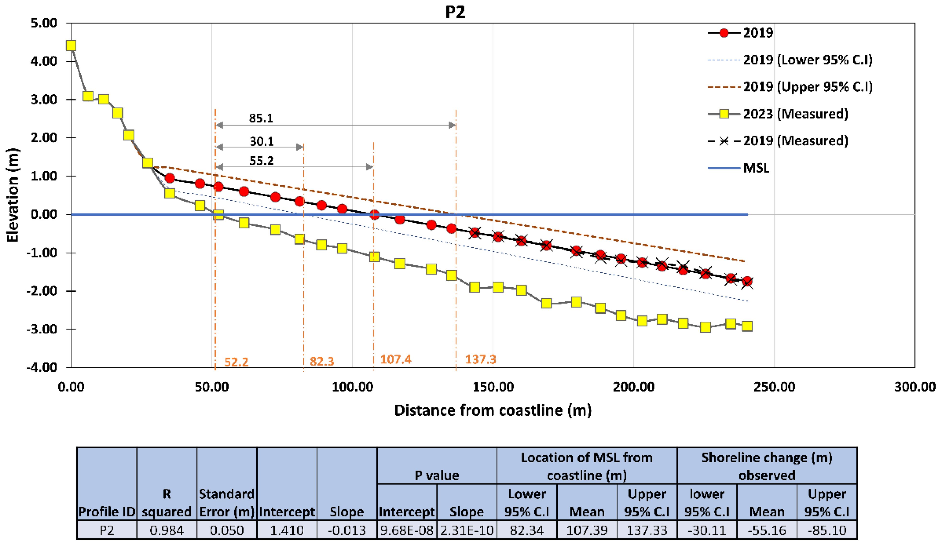
Figure 16. Illustration of the estimated shoreline and the uncertainty range at point 2. Summary statistics of all points are given in Table 5.

The quantitative summary of comparison between the new approach and the conventional approach is shown in Figure 17. The overestimation of the landward shift of the shoreline is observed in the conventional approach. The nearshore bathymetry of profiles (P1–P3) is uniform alongshore, which results in less significant difference in capturing the pattern of erosion from both approaches. However, the conventional approach shows overestimation of erosion due to the difference in DoC considered. Notably, the new approach shows greater improvement at P4, P5, and P6 relative to the conventional approach, where the bathymetry is nonuniform alongshore and the reef is present. This highlights the significance of the current approach.

Figure 17

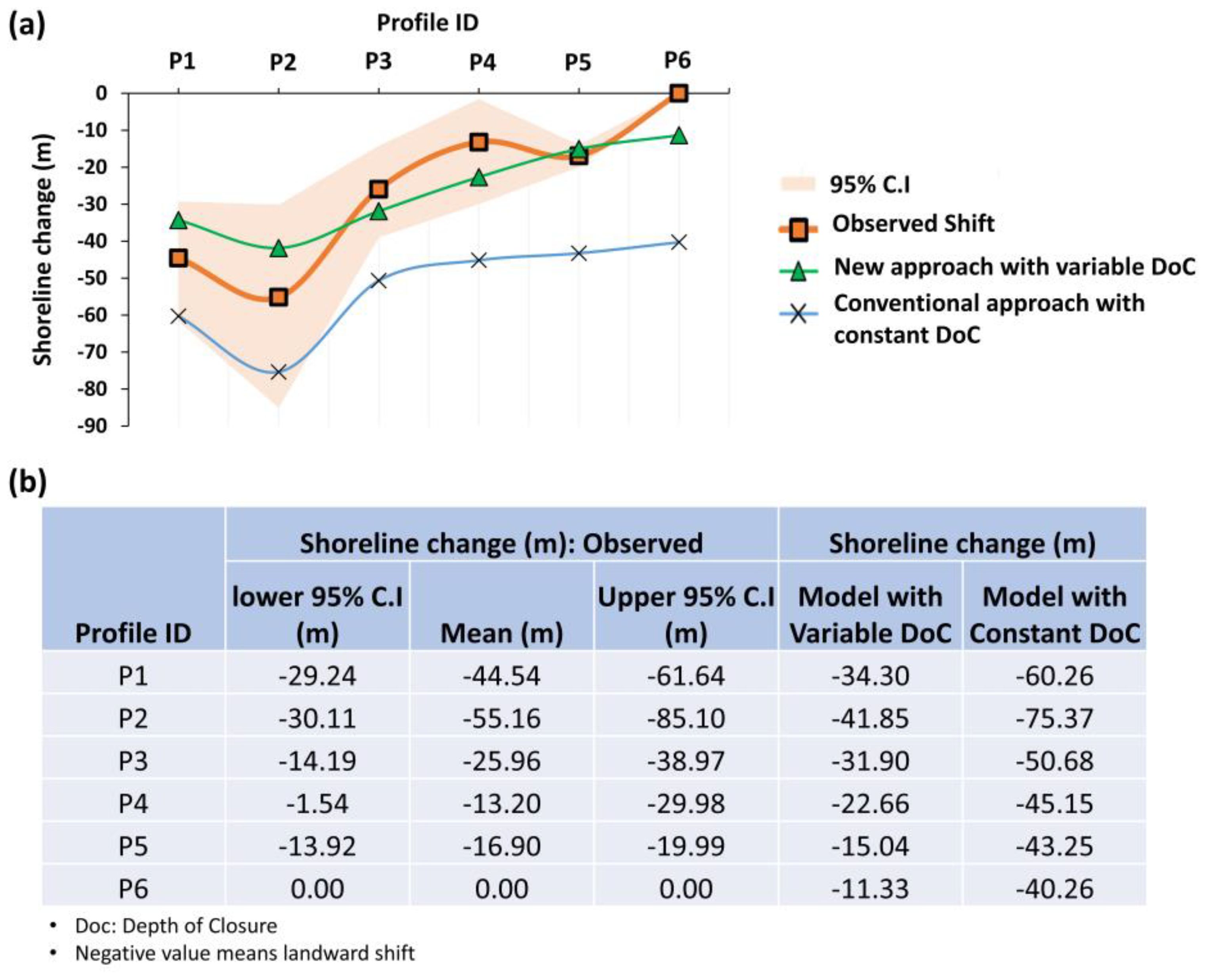
Figure 17. Comparison summary of the new approach (variable depth of closure) and the conventional approach (constant depth of closure); (A) graphical summary and (B) quantitative summary.

5 Conclusions and recommendations

Hybrid 2D/one-line shoreline evolution models are becoming increasingly popular over the traditional 2DH methods to inform the management of sandy coastal systems. The computational framework adapted in this study, i.e., a hybrid 2D/one-line shoreline model, is superior to the traditional 2DH-only models, with the main computational difference between them being the shoreline morphology update. The 2DH models update the morphology across the entire domain at each time step, and the change in morphology from one time step updates the mesh bathymetry for the next time-step, to continue the simulation. The hybrid 2D/one-line models maintain the same principles as 2DH models, except they constrain the morphology update within the limits of the active coastal profile.

The most significant findings derived from this study are summarized below:

● The optimal boundary conditions for simulating shoreline evolution are linked to observed coastal system morphology and processes, especially in complex morphological regions.

● The nearshore bathymetry that defines the mesh resolution in the nearshore is an important addition to any regional model as the near-accurate wave conditions define the depth of closure calculations for better sediment transport and shoreline prediction studies.

● The hybrid 2D/one-line modeling approach used in the present study is restricted to simple planform morphologies as tested here. This is plausibly attributed to the use of the one-line theory assumption that the active coastal profile maintains a constant time-averaged form and vertical limits (depth of closure).

Some future research recommendations based on this study are listed below:

1. Expanding model applicability to complex morphologies

While the current study’s hybrid 2D/one-line shoreline model performs well for simple planform morphologies, future research should focus on extending this approach to more complex coastal settings, such as highly curved shorelines, multiple inlets, and regions with varying bathymetric features.

2. Long-term model calibration and validation

Extending the timescales of model simulations and calibrations could help in evaluating the long-term performance and stability of the hybrid 2D/one-line models. Future studies should consider long-term datasets (including changes in wave directions) to improve model robustness and applicability over decadal timescales.

3. User-friendly and computationally efficient implementations

To encourage widespread adoption by coastal managers and practitioners, future efforts should aim at creating user-friendly interfaces and reducing computational costs of hybrid models.

These recommendations aim to address current limitations while exploring new opportunities for improving the performance and applicability of hybrid shoreline evolution models in diverse coastal environments.

Data availability statement

The original contributions presented in the study are included in the article/supplementary material. Further inquiries can be directed to the corresponding author.

Author contributions

NL: Methodology, Writing – original draft, Writing – review & editing, Data curation, Formal analysis, Software. PC: Methodology, Writing – original draft, Writing – review & editing, Conceptualization, Funding acquisition, Project administration, Supervision. MB: Formal analysis, Methodology, Writing – original draft, Writing – review & editing.

Funding

The author(s) declare financial support was received for the research, authorship, and/or publication of this article. Funded by DSIT (Department for Science, Innovation and Technology), Government of UK through The Tactical Fund number C8556 770 “Machine learning based improved local wave climate prediction for sediment transport 771 modeling to obtain smart maps for coastal zone management”.

Acknowledgments

PC wishes to thank DSIT (Department for Science, Innovation and Technology), Government of UK for funding this study through The Tactical Fund number C8556 “Machine learning based improved local wave climate prediction for sediment transport modeling to obtain smart maps for coastal zone management”. The authors wish to thank Dr. Paulette Posen for her valuable feedback on the draft manuscript.

Conflict of interest

The authors declare that the research was conducted in the absence of any commercial or financial relationships that could be construed as a potential conflict of interest.

Publisher’s note

All claims expressed in this article are solely those of the authors and do not necessarily represent those of their affiliated organizations, or those of the publisher, the editors and the reviewers. Any product that may be evaluated in this article, or claim that may be made by its manufacturer, is not guaranteed or endorsed by the publisher.

References

Aboobacker V. M., Vethamony P., Rashmi R. (2011). Shamal” swells in the Arabian Sea and their influence along the west coast of India. Geophys Res. Lett. 38, 1–7. doi: 10.1029/2010GL045736

Crossref Full Text | Google Scholar

Anderson J. R. (2007). “Sand sieve analysis,” in Pamela JW Gore “Historical Geology Online Laboratory Manual, 278.

Google Scholar

Aragonés L., Pagán J. I., López I., Serra J. C. (2018). Depth of closure: New calculation method based on sediment data. Int. J. Sediment Res. 33, 198–207. doi: 10.1016/j.ijsrc.2017.12.001

Crossref Full Text | Google Scholar

Ashton A., Murray A. B., Arnoult O. (2001). Formation of coastline features by large-scale instabilities induced by high-angle waves. Nature 414, 296–300. doi: 10.1038/35104541

PubMed Abstract | Crossref Full Text | Google Scholar

Ashton A. D., Murray A. B. (2006). High-angle wave instability and emergent shoreline shapes: 1. Modeling of sand waves, flying spits, and capes. J. Geophysical Research: Earth Surface 111, 1–19. doi: 10.1029/2005JF000422

Crossref Full Text | Google Scholar

Barnard P. L., van Ormondt M., Erikson L. H., Eshleman J., Hapke C., Ruggiero P., et al. (2014). Development of the Coastal Storm Modeling System (CoSMoS) for predicting the impact of storms on high-energy, active-margin coasts. Natural hazards 74, 1095–1125. doi: 10.1007/s11069-014-1236-y

Crossref Full Text | Google Scholar

Battjes J. A., Janssen J. P. F. M. (1978). Energy loss and set-up due to breaking of random waves. Coast. Eng. 1978, 569–587. doi: 10.1061/9780872621909.034

Crossref Full Text | Google Scholar

Bruun P. (1962). Sea-level rise as a cause of shore erosion. J. Waterw. Harb.Div. 88, 117–132. doi: 10.1061/JWHEAU.0000252

Crossref Full Text | Google Scholar

Chowdhury P., Behera M. R. (2017). Effect of long-term wave climate variability on longshore sediment transport along regional coastlines. Prog. Oceanography 156, 145–153. doi: 10.1016/j.pocean.2017.06.001

Crossref Full Text | Google Scholar

Chowdhury P., Behera M. R. (2018). Evaluation of CMIP5 and CORDEX derived wave climate in Indian Ocean. Climate Dynamics 52, 4463–4482. doi: 10.1007/s00382-018-4391-0

Crossref Full Text | Google Scholar

Chowdhury P., Behera M. R. (2019). “Nearshore sediment transport in a changing climate,” in Climate Change Signals and Response: A Strategic Knowledge Compendium for India. Eds. Venkataraman C., Mishra T., Ghosh S., Karmakar S. (Singapore: Springer Singapore), 147–160. doi: 10.1007/978-981-13-0280-0_9

Crossref Full Text | Google Scholar

Chowdhury P., Behera M. R., Reeve D. E. (2019). Wave climate projections along the Indian coast. Int. J. Climatol. 39, 4531–4542. doi: 10.1002/joc.6096

Crossref Full Text | Google Scholar

Chowdhury P., Behera M. R., Reeve D. E. (2020). Future wave-climate driven longshore sediment transport along the Indian coast. Climatic Change 162, 405–424. doi: 10.1007/s10584-020-02693-7

Crossref Full Text | Google Scholar

Chowdhury P., Lakku N. K. G., Lincoln S., Seelam J. K., Behera M. R. (2023). Climate change and coastal morphodynamics: Interactions on regional scales. Sci. Total Environ. 899, 166432. doi: 10.1016/j.scitotenv.2023.166432

PubMed Abstract | Crossref Full Text | Google Scholar

Davidson M. A., Lewis R. P., Turner I. L. (2010). Forecasting seasonal to multi-year shoreline change. Coast. Eng. 57, 620–629. doi: 10.1016/j.coastaleng.2010.02.001

Crossref Full Text | Google Scholar

de Winter R. C., Gongriep F., Ruessink B. G. (2015). Observations and modeling of alongshore variability in dune erosion at Egmond aan Zee, the Netherlands. Coast. Eng. 99, 167–175. doi: 10.1016/j.coastaleng.2015.02.005

Crossref Full Text | Google Scholar

DHI (2024). Littoral Processes FM, All Modules (Denmark: Scientific Documentation).

Google Scholar

Engelund F., Fredsoe J. (1976). A sediment transport model for straight alluvial channels. IWA Publishing. 293–306. doi: 10.2166/nh.1976.0019

Crossref Full Text | Google Scholar

Erikson L. H., Hegermiller C. A., Barnard P. L., Ruggiero P., van Ormondt M. (2015). Projected wave conditions in the Eastern North Pacific under the influence of two CMIP5 climate scenarios. Ocean Model. 96, 171–185. doi: 10.1016/j.ocemod.2015.07.004

Crossref Full Text | Google Scholar

Ferreira A. M., Coelho C., Silva P. A. (2024). Medium-term effects of dune erosion and longshore sediment transport on beach–dune systems evolution. J. Mar. Sci. Eng. 12, 1083. doi: 10.3390/jmse12071083

Crossref Full Text | Google Scholar

Fletcher C., Rooney J., Barbee M., Lim S. C., Richmond B. (2003). Mapping shoreline change using digital orthophotogrammetry on Maui, Hawaii. J. Coast. Res., 106–124. Available online at: http://www.jstor.org/stable/25736602

Google Scholar

Fredsøe J. (1984). Turbulent boundary layer in wave-current motion. J. Hydraul. Eng. 110, 1103–1120. doi: 10.1061/(ASCE)0733-9429(1984)110:8(1103)

Crossref Full Text | Google Scholar

Fredsøe J., Andersen O. H., Silberg S. (1985). Distribution of suspended sediment in large waves. J. Waterw. Port Coastal Ocean Eng. 111, 1041–1059. doi: 10.1061/(asce)0733-950x(1985)111:6(1041

Crossref Full Text | Google Scholar

Glejin J., Sanil Kumar V., Balakrishnan Nair T. M., Singh J. (2013). Influence of winds on temporally varying short and long period gravity waves in the near shore regions of the eastern Arabian Sea. Ocean Sci. 9, 343–353. doi: 10.5194/os-9-343-2013

Crossref Full Text | Google Scholar

Hallermeier R. J. (1979). Uses for a calculated limit depth to beach erosion. Proc. Coast. Eng. Conf. 2, 1493–1512. doi: 10.9753/icce.v16.88

Crossref Full Text | Google Scholar

Hallermeier R. J. (1981). A profile zonation for seasonal sand beaches from wave climate. Coast. Eng. 4, 253–277. doi: 10.1016/0378-3839(80)90022-8

Crossref Full Text | Google Scholar

Hasselmann K. (1974). On the spectral dissipation of ocean waves due to white capping. Boundary-Layer Meteorol. 6, 107–127. doi: 10.1007/BF00232479

Crossref Full Text | Google Scholar

Hegermiller C. A., Erikson L. H., Barnard P. L. (2016). Nearshore waves in Southern California: Hindcast, and modeled historical and 21st-century projected time series: U.S (Geological Survey data release) (Accessed 15 April 2024).

Google Scholar

Hemer M. A., Fan Y., Mori N., Semedo A., Wang X. L. (2013). Projected changes in wave climate from a multi-model ensemble. Nat. Clim. Change 3, 471–476. doi: 10.1038/nclimate1791

Crossref Full Text | Google Scholar

Houston J. R. (1996). Simplified Dean's method for beach-fill design. J. waterway port coastal ocean Eng. 122, 143–146. doi: 10.1061/(ASCE)0733-950X(1996)122:3(143)

Crossref Full Text | Google Scholar

Kaergaard K., Fredsoe J. (2013). A numerical shoreline model for shorelines with large curvature. Coast. Eng. 74, 19–32. doi: 10.1016/j.coastaleng.2012.11.011

Crossref Full Text | Google Scholar

Komen G. J., Cavaleri L., Donelan M., Hasselmann K., Hasselmann S., Janssen P. A. E. M. (1994). Dynamics and Modelling of Ocean Waves (New York: Cambridge University Press). doi: 10.1017/CBO9780511628955

Crossref Full Text | Google Scholar

Komen G. J., Janssen P. A. E. M., Makin V. K., Mastenbroek C., Oost W. A. (1998). On the sea state dependence of the Charnock parameter. Global Atmos. Ocean Syst. 5, 367–388.

Google Scholar

Kraus N. C., Larson M., Wise R. A. (1999). “Depth of closure in beach fill design,” in Proceedings of the 1999 National Conference on Beach Preservation Technology (FSBPA, Tallahassee, Florida), 268–280.

Google Scholar

Kristensen S. E., Drønen N., Deigaard R., Fredsoe J. (2013). Hybrid morphological modelling of shoreline response to a detached breakwater. Coast. Eng. 71, 13–27. doi: 10.1016/j.coastaleng.2012.06.005

Crossref Full Text | Google Scholar

Larson M. (1991). “Equilibrium profile of a beach with varying grain size,” in Proceedings Coastal Sediments 1991 (ASCE, Seattle, Washington), 861–874.

Google Scholar

Larson M., Hanson H., Kraus N. C. (1997). Analytical solutions of one-line model for shoreline change near coastal structures. J. Waterw. Port Coast. Ocean Eng. 123, 180–191. doi: 10.1061/(ASCE)0733-950X(1997)123:4(180)

Crossref Full Text | Google Scholar

Long J. W., Plant N. G. (2012). Extended Kalman filter framework for forecasting shoreline evolution. Geophys. Res. Lett. 39, L13603. doi: 10.1029/2012GL052180

Crossref Full Text | Google Scholar

Mason D. C., Scott T. R., Dance S. L. (2010). Remote sensing of intertidal morphological change in Morecambe Bay, UK, between 1991 and 2007. Estuarine Coast. Shelf Sci. 87, 487–496. doi: 10.1016/j.ecss.2010.01.015

Crossref Full Text | Google Scholar

Miller J. K., Dean R. G. (2004). A simple new shoreline change model. Coast. Eng. 51, 531–556. doi: 10.1016/j.coastaleng.2004.05.006

Crossref Full Text | Google Scholar

Murray A. B. (2007). Reducing model complexity for explanation and prediction. Geomorphology 90, 178–191. doi: 10.1016/j.geomorph.2006.10.020

Crossref Full Text | Google Scholar

Nicholls R. J., Birkemeier W. A., Hallermeier R. J. (1996). Application of the depth of closure concept. Coast. Eng., 3874–3887. doi: 10.1061/9780784402429.299

Crossref Full Text | Google Scholar

Noujas V., Kankara R. (2018). “Shoreline prediction using a numerical model along rathnagiri coast, West Coast of India,” in 6th National Conference on Coastal, Harbour and Ocean Engineering (INCHOE 2018). Pune, India: CWPRS (Accessed September 26-28, 2018).

Google Scholar

Pape L., Kuriyama Y., Ruessink B. G. (2010). Models and scales for cross-shore sandbar migration. J. Geophys. Res. 115. doi: 10.1029/2009JF001644

PubMed Abstract | Crossref Full Text | Google Scholar

Payo A., Hall J. W., French J., Sutherland J., van Maanen B., Nicholls R. J., et al. (2016). Causal loop analysis of coastal geomorphological systems. Geomorphology 256, 36–48. doi: 10.1016/j.geomorph.2015.07.048

Crossref Full Text | Google Scholar

Quadrado G. P., Goulart E. S. (2020). Longshore sediment transport: predicting rates in dissipative sandy beaches at southern Brazil. SN Appl. Sci. 2, 1421. doi: 10.1007/s42452-020-03223-x

Crossref Full Text | Google Scholar

Ranasinghe R. (2016). Assessing climate change impacts on open sandy coasts: A review. Earth Sci. Rev. 160, 320–332. doi: 10.1016/j.earscirev.2016.07.011

Crossref Full Text | Google Scholar

Ranasinghe R. W. M. R. J. B., Callaghan D., Roelvink D. (2013). “Does a more sophisticated storm erosion model improve probabilistic erosion estimates?,” in Coastal Dynamics 2013: 7th International Conference on Coastal Dynamics, Arcachon, France, 24-28 June 2013.

Google Scholar

Rao V. R., Murthy M. R., Bhat M., Reddy N. T. (2009). Littoral sediment transport and shoreline changes along Ennore on the southeast coast of India: Field observations and numerical modeling. Geomorphology 112, 158–166. doi: 10.1016/j.geomorph.2009.05.015

Crossref Full Text | Google Scholar

Reimann L., Vafeidis A. T., Honsel L. E. (2023). Population development as a driver of coastal risk: Current trends and future pathways Vol. 1 (New York: Cambridge Prisms, Coastal Futures).

Google Scholar

Remya P. G., Kumar R., Basu S., Sarkar A. (2012). Wave hindcast experiments in the Indian Ocean using MIKE 21 SW model. J. Earth System Sci. 121, 385–392. doi: 10.1007/s12040-012-0169-7

Crossref Full Text | Google Scholar

Roelvink D., Reniers A. J. H. M., Van Dongeren A., Van Thiel de Vries J., Lescinski J., McCall R. (2010). XBeach model description and manual (Amsterdam: Unesco-IHE Institute for Water Education, Deltares and Delft University of Technology).

Google Scholar

Roelvink J. A., Van Banning G. K. F. M. (1995). Design and development of DELFT3D and application to coastal morphodynamics. Oceanogr. Lit. Rev. 11, 925.

Google Scholar

Scott T., McCarroll R. J., Masselink G., Castelle B., Dodet G., Saulter A., et al. (2021). Role of atmospheric indices in describing inshore directional wave climate in the United Kingdom and Ireland. Earth's Future 9, 1–21. doi: 10.1029/2020EF001625

Crossref Full Text | Google Scholar

Shetty A., Jayappa K. S. (2020). Seasonal variation in longshore sediment transport rate and its impact on sediment budget along the wave-dominated Karnataka coast, India. J. Earth System Sci. 129, 1–14. doi: 10.1007/s12040-020-01504-y

Crossref Full Text | Google Scholar

Shope J. B., Storlazzi C. D., Erikson L. H., Hegermiller C. A. (2016). Changes to extreme wave climates of islands within the Western Tropical Pacific throughout the 21st century under RCP 4.5 and RCP 8.5, with implications for island vulnerability and sustainability, Global Planet. Change 141, 25–38. doi: 10.1016/j.gloplacha.2016.03.009

Crossref Full Text | Google Scholar

Simm J. D. (Ed.) (1996). Beach Management Manual Vol. 153 (London: CIRIA, CIRIA Report), 448p.

Google Scholar

Smagorinsky J. (1963). General circulation experiments with the primitive equations: I. The basic experiment. Mon. Weather Rev. 91, 99–164. doi: 10.1175/1520-0493(1963)091<0099:GCEWTP>2.3.CO;2

Crossref Full Text | Google Scholar

Sørensen O. R., Kofoed-Hansen H., Rugbjerg M., Sørensen L. S. (2004). “A third generation spectral wave model using an unstructured finite volume technique,” in Proceedings of the 29th International Conference on Coastal Engineering, ICCE, Lisbon, Portugal, 19–24 September 2004. 894–906. doi: 10.1142/9789812701916_0071

Crossref Full Text | Google Scholar

Splinter K. D., Turner I. L., Davidson M. A., Barnard P., Castelle B., Oltman-Shay J. (2014). A generalized equilibrium model for predicting daily to interannual shoreline response. J. Geophys. Res. Earth 119, 1936–1958. doi: 10.1002/2014JF003106

Crossref Full Text | Google Scholar

Stive M. J. F., De Vriend H. J., Nicholls R. J., Capobianco M. (1992). “Shore nourishment and the active zone: a timescale dependent view,” in Proceedings of the 23rd Coastal Engineering Conference, New York: American Society of Civil Engineers. 2464–2473.

Google Scholar

Ton A. M., Vuik V., Aarninkhof S. G. (2023). Longshore sediment transport by large-scale lake circulations at low-energy, non-tidal beaches: A field and model study. Coast. Eng. 180, 104268. doi: 10.1016/j.coastaleng.2022.104268

Crossref Full Text | Google Scholar

Van Dongeren A., Bolle A., Vousdoukas M. I., Plomaritis T., Eftimova P., Williams J., et al. (2009). “MICORE: dune erosion and overwash model validation with data from nine European field sites,” in Proceedings Of Coastal Dynamics 2009: Impacts of Human Activities on Dynamic Coastal Processes (World Scientific), 1–15.

Google Scholar

Venugopal V., Smith G. H. (2007). “Wave climate investigation for an array of wave power devices,” in Proceedings of the 7th European wave and tidal energy conference, Porto, Portugal. 1–10.

Google Scholar

Vinod Kumar K., Aboobacker V. M., Saheed P. P., Vethamony P. (2012). Coastal circulation along the central west coast of India during cyclone Phyan: Measurements and numerical simulations. Nat. Hazards 64, 259–271. doi: 10.1007/s11069-012-0228-z

Crossref Full Text | Google Scholar

Warner J. C., Armstrong B., He R., Zambon J. B. (2010). Development of a coupled ocean–atmosphere–wave–sediment transport (COAWST) modeling system. Ocean Model. 35, 230–244. doi: 10.1016/j.ocemod.2010.07.010

Crossref Full Text | Google Scholar

Warren I. R., Bach H. (1992). MIKE 21: A modelling system for estuaries, coastal waters and seas. Environ. Software 7, 229–240. doi: 10.1016/0266-9838(92)90006-P

Crossref Full Text | Google Scholar

Warrick J. A., Mertes L. A. (2009). Sediment yield from the tectonically active semiarid Western Transverse Ranges of California. Geol. Soc Am. Bull. 121, 1054–1070. doi: 10.1130/B26452.1

Crossref Full Text | Google Scholar

Work P. A., Dean R. G. (1991). “Effect of varying sediment size on equilibrium beach profiles,” in Proceedings Coastal Sediments 1991 (ASCE, Seattle, Washington), 891–904.

Google Scholar

Zacharioudaki A., Reeve D. E. (2011). Shoreline evolution under climate change wave scenarios. Climatic Change 108, 73–105. doi: 10.1007/s10584-010-0011-7

Crossref Full Text | Google Scholar

Zarifsanayei A. R., Etemad-Shahidi A., Cartwright N., Strauss D. (2020). Long-term prediction of longshore sediment transport in the context of climate change. Coast. Eng. Proc. 36, 15–15. doi: 10.9753/icce.v36v.papers.15

Crossref Full Text | Google Scholar