Impact of the ocean in-situ observations on the ECMWF seasonal forecasting system

This study aims to evaluate the impact of the in-situ ocean observations on seasonal forecasts. A series of seasonal reforecasts have been conducted for the period 1993-2015, in which different sets of ocean observations were withdrawn in the production of the ocean initial conditions, while maintaining a strong constrain in sea surface temperature (SST). By comparing the different reforecast sets, it is possible to assess the impact on the forecast of ocean and atmospheric variables. Results show that the in-situ observations have profound and significant impacts on the mean state of forecast ocean and atmospheric variables, which can be classified into different categories: i) impact due to local air-sea interaction, as direct consequence of changes in the mixed layer in the ocean initial conditions, and visible in the early stages of the forecasts; ii) changes due to different ocean dynamical balances, most visible in the Equatorial Pacific in forecasts initialized in May, which amplify and evolve with forecast lead time; iii) changes to the atmospheric circulation resulting from changes in large scale SST gradients; these are non-local, mediated by the atmospheric bridge, and they are obvious from the visible impact of the removing in-situ observations on the Atlantic basin only in the global atmospheric circulation; iv) changes in the atmospheric tropical deep convection associated with the structure of the warm pools. The ocean observations have also a significant impact on the representation of the trends of the ocean initial conditions, which affect the trends in the seasonal forecasts of ocean and atmospheric variables. The impact of the ocean observing system in the Atlantic and extratropics appears dominated by Argo, but this is not the case in the Tropical Pacific, where the other ocean observing systems play a role in constraining the ocean state.

1 Introduction

There is increasing demand for the evaluation of the global ocean observing system (GOOS, 2018), as the number of societal applications that rely on ocean observations multiply and the observational capabilities expand. The ocean observing system has undergone a dramatic transformation in the past 30 years and there are ambitious prospects for its expansion (Moltman and co-authors, 2019). Applications range from short-range marine forecasting at regional to global scale, climate reanalyzes, fresh-water and energy budget, and seamless weather and climate forecasts, and domain specific efforts for assessing the observing systems are ongoing (see Fujii and co-authors, 2019 for a review). The work presented here is concerned with the evaluation of the subsurface ocean observing system from a seasonal forecast perspective. This is a companion paper of Balan-Sarojini et al. (2024) (this issue), who report the impact of ocean observations on subseasonal time scales.

Seasonal forecasting is currently a routine activity in several operational centers, with a growing number of economic and societal applications in fields such as agriculture, health, and energy. Seasonal forecasts predict variations in the atmospheric circulation in response to anomalous boundary forcing, which significantly changes the probability of occurrence of weather patterns (Palmer and Anderson, 1994). Sea surface temperature (SST) variations are the most dominant source of boundary forcing. Of special importance are the variations of the tropical SST associated with El Niño Southern Oscillation (ENSO), which have the potential to alter the worldwide large-scale atmospheric circulation associated with variations in the tropical convective cells (Goddard and Dilley, 2005; Goddard and Graham, 1999). Variations in tropical SST other than those related to ENSO can also drive temperature and precipitation anomalies on seasonal timescales (Folland et al., 2001; Giannini et al., 2003; Rodwell and Folland, 2002; Saji et al., 1999, among others). Realizing the potential predictability at seasonal time scales depends critically on the adequacy of initial conditions for the ocean component of the coupled models used for prediction, which in turn depends on the adequacy of the ocean observing system (Balmaseda, 2017 and references therein).

One method often used to evaluate the impact of ocean observations on seasonal forecasts is what we called evaluation by temporal sub-sampling. This consists in comparing the performance for seasonal reforecasts among time periods chosen to represent different scenarios of observation coverage (Kumar et al., 2015; Huang et al., 2017). These way of assessing the observing system requires sufficiently long records of reforecasts -around 40 years or more- so different temporal samples of sufficient length (10 to 20 years) can be extracted. As such this is a method of opportunity, which takes the advantage of the existing long reforecasts records to gain insight into the value of observations. It assumes that the skill of the system is stationary, and that the only variations in the chosen impact metric comes from variations in the observing system. In the case of seasonal forecasts this is arguably too strong an assumption, since the interannual variability and seasonal forecast skill can be modulated by low frequency climate variations (e.g., Balmaseda et al., 1995; Torrence and Webster, 1998). An alternative method, used less frequently because of the computation cost, is to conduct Observing System Experiments (OSEs), in which different sets of seasonal reforecasts from a collection of dates -spanning the same period - are initialized by ocean initial conditions produced by withholding a selected subset of the observing system (Balmaseda and Anderson, 2009; Balmaseda et al., 2010; Fujii et al., 2011, 2015; Xue et al., 2017). This is the methodology followed in this work.

Here we use a series of Observing System Experiments to evaluate the impact of subsurface ocean observations on the ECMWF seasonal forecasting system SEAS5 (Johnson et al., 2019). A novel aspect of the work presented here is that the evaluation extends to the impact on the global domain on both ocean and atmospheric variables. The assessment includes the impact of all in-situ observations and the impact of only Argo (Roemmich and co-authors, 2019 and references therein). Because of the importance of the tropical SST for seasonal forecasts, and because the Tropical Pacific Observing System (TPOS) is undergoing a transformation (Kessler et al., 2021), we pay special attention to how the ocean initial conditions impact the forecasts of tropical SST. To quantify the impact on the seasonal forecasts of the global atmosphere of observations in basins outside the Pacific, we also conduct a regional experiment, removing all the in-situ observations in the Atlantic basin. The assessment in this paper focuses on changes in the mean state and linear trends. The mean state is important because often these initialized forecasts are used to evaluate coupled model errors, and these errors may depend on the ocean initialization. The analysis of trends is relevant for two reasons: i) the current calibration of seasonal forecasts assumes that the errors are stationary, and changes in the ocean observing system may affect this assumption if the ocean observing system impacts the trends; ii) in a changing climate it is important to quantify, forecast and understand how the climate changing is evolving in response to greenhouse gasses, and the ocean observing system plays a pivotal role. Assimilation of ocean observations also impacts forecast skill, but as discussed in Methods below that is not the focus of this study.

The paper is organized as follows: section 2 describes the experimental set up and describes the evaluation methodology; section 3 presents the resulting impact of withdrawing subsurface observations in the initial conditions, and how this affects the mean state and trends of seasonal forecasts of ocean and atmospheric variables. Section 4 summarizes the main outcomes.

2 Methods

2.1 Experiment description

The observing system experiments used to assess the impact of subsurface ocean observations information consists of two distinctive steps: 1) the production of sets of ocean initial conditions by conducting a series of ocean and sea-ice reanalyzes experiments (ORA-OSEs), which only differ on the amount of ocean observations assimilated; and 2) the production of a set of retrospective seasonal forecast (reforecast) experiments (FC-OSEs), initialized from the respective ORA-OSEs. Both the ORA and FC OSES are conducted respectively with a low-resolution variant of the currently operational ocean reanalysis ORAS5 (Zuo et al., 2019) and seasonal forecast system SEAS5 (Johnson et al., 2019). Table 1 provides a summary of the experiments conducted.

Table 1

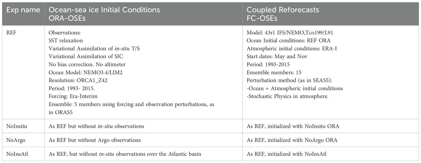
Table 1. Details of the OSE conducted.

The ORA-OSE experiments are the same as those reported by Zuo et al. (2019), and Balan-Sarojini et al. (this issue). They are produced with the same ocean and sea-ice model versions (NEMO v3.4.1 and LIM2), forcing fields from Era-Interim (Dee and co-authors, 2011), 3D-variational assimilation procedure and ensemble generation method as ORAS5, but at lower horizontal and vertical resolution: the ORA-OSEs use the ORCA1_Z42 levels which is has an approximate horizontal grid spacing of 1 degree (with meridional refinement at the Equator, where the latitudinal grid refinement is about 1/3 degree), and 42 levels in the vertical, with upper ocean level thickness of 10 meters. Another important difference with ORAS5 is that in these experiments the bias correction and assimilation of altimeter sea level has been switched off. This allows cleaner interpretation of the impact on ocean observations, since both the bias correction and altimeter assimilation indirectly require information from the in-situ observations. For example, to assimilate sea-level anomalies ancillary information about the mean dynamic topography (MDT) is required. The MDT field in ORAS5 is obtained from by temporal averaging of the sea surface height field from a reanalysis experiment where in-situ observations have been assimilated. This implies that the information from in-situ observations is indirectly used when assimilating altimeter data. The same argument applies for the bias correction applied in ORAS5, which is obtained from the assimilation increments of a previous experiment that assimilates all in-situ observations.

As for ORAS5, the in-situ temperature and salinity (T/S) profiles come in the ORA-OSE from the quality-controlled data set EN4 (Good et al., 2013) with expendable bathythermograph (XBT) and mechanical bathythermograph (MBT) depth corrections from Gouretski and Reseghetti (2010) until May 2015. The reference experiment (REF) was carried out by assimilating all in situ observations from the quality-controlled EN4 data set with the multivariate 3D-variational method NEMOVAR, as described in Zuo et al. (2019). From the same initial conditions of ORA REF in 1993, three additional experiments were conducted: (1) ORA NoInsitu – removing all in situ observations; (2) ORA NoArgo – removing Argo floats; and (3) ORA NoInsAtl – removing all in situ observations in the Atlantic basin only. All the ORA OSE experiments maintain the SST constrain, which is effectively a strong relaxation (200 W/m2/K) to the SST field used to constrain ORAS5, and the variational assimilation of sea-ice concentration (SIC). The ORA-OSE consist on 5 ensemble members, created with the same perturbation methodology as in ORAS5 (see section 1 of Supplementary Material for more details).

The ORA OSEs are used to initialize respective sets of seasonal reforecasts spanning the period 1993-2015, starting in May and November. Forecasts for each individual month and year comprise 15 ensemble members, generated as in SEAS5 (Johnson et al., 2019, see also section 1 in Supplementary Material). We call these experiments FC-OSEs. The coupled model is based on the ECMWF’s Integrated Forecasting System (IFS) atmosphere model cycle 43r1 coupled to the NEMO v3.4.1 ocean model LIM2 sea-ice model. Atmosphere and land are initialized from the European Interim Re-Analysis (ERA-Interim; Dee and co-authors, 2011). The ocean resolution is the same as the ORA-OSEs. The atmospheric resolution of the FC-OSES is Tco199 (as opposed to Tco319 in the operational SEAS5). The vertical resolution is 91 levels, the same as SEAS5. The atmospheric resolution and the atmospheric model version are the main differences between the FC-OSEs used here for the seasonal evaluation and those in Balan-Sarojini et al. (2024) to evaluate the observation impact on subseasonal forecasts. Results from the latter OSEs on specific processes relevant for the subseasonal time scales have also been reported by Du et al. (2023) and Wei et al. (2023), but this is the first time that results are presented for the seasonal time scales.

2.2 Evaluation method

The evaluation methodology consists in measuring the differences in the mean climate and linear trends between a given OSE with respect to the REF experiment. The impact on the mean is done for the period 2005-2015, an 11-year period corresponding with the full maturity of the Argo observing system. The results for this period are qualitatively similar to those obtained for the longer 23-year period 1993-2015. In the period before 2004, REF and NoArgo assimilate the same observations, and therefore are equivalent. For the period after 2005, differences between NoInsitu and NoArgo during the longer period arise from two contributions: i) the impact of in-situ observations prior to the Argo period, and ii) the impact of other in situ observations different from Argo during the Argo period. Analysis of additional experiments where the moorings and the XBTs were removed suggest that after 2005 the impact of other in-situ observations is small. To evaluate the impact on the linear trends, we use the period 1993-2015, since this is close to the period used by other studies to evaluate the errors in the trends in seasonal forecasts (Balmaseda et al., 2024). The trend and its significance are estimated using a simple regression model. The significance of the differences in mean and trend is obtained via a paired t-test, from the samples of simultaneous pairs of differences between the OSE and REF experiments.

For the ORA-OSES we analyze the impact on variables with potential to impact the SST in the coupled forecasts via a variety of processes: depth of the 20 degree isotherm (D20I), as a proxy for thermocline depth in the tropics, which is relevant for equatorial wave propagation and ENSO prediction; depth of 28 degrees isotherm (D28I), as a proxy for the depth of the warm pools, which may affect deep tropical convection at short and long lead times; mixed layer depth (MLD, estimated as the ocean layer where the differences in density with respect the ocean surface exceeds the 0.001 kg/m3), since it affects the exchange of air-sea fluxes; ocean heat content in the upper 300m (OHC); barotropic stream function (BarStf), which illustrates changes in circulation likely to affect timescales longer than a few months; and sea surface height (SSH), which encompasses changes in upper ocean heat content, thermocline depth in the tropics and circulation changes. In keeping with our focus on low-frequency changes, statistics from the ocean reanalyzes are shown in terms of annual means. For the forecasts, the ensemble mean of FC-OSES is used to evaluate the statistics for each starting month (November or May starts) and for each lead season (one and two seasons ahead) separately. The ocean variables analyzed are SST, OHC, D28I and MLD. For the atmosphere we analyze temperature at 2m above the surface (T2m), total precipitation (TP), mean sea level pressure (MSL), geopotential height at 500hPa (Z500) and zonal winds at 850 hPa and 200 hPa (U850 and U200 respectively). The significance of the differences in mean and trend is obtained via a paired t-test, from the samples of simultaneous pairs of differences between the OSE and REF experiments.

We also conduct a linear multivariate perturbation analysis to explore how the ocean initial conditions perturbations translate into differences in the forecasts of SST over the tropical area. To increase the sample size and to include a range of temporal variations, we construct sets of initial δIni and forecast δFc perturbations by aggregating pairs of differences between pairs of experiments, each of them spanning the record 1993-2015 (i.e. 23 years). The ocean initial perturbations δIni for a given forecast start month (May or November) are constructed by aggregating contemporaneous differences between N pairs of ORA experiments, yielding a sample size of N x 23 for a given forecast start month. The forecast perturbations δFc are constructed in similar manner by collating pairs of differences from the ensemble mean of corresponding FC-OSES, and they depend on the forecast lead time. Local correlation analysis and multivariate singular value decomposition between δIni and δFc are conducted to explore how the initial uncertainty manifests on forecast uncertainty. For more details see the section 2 in Supplementary Material. We conduct three different perturbation analysis:

● The main analysis uses the pairs (NoInsitu-REF, NoArgo-REF, NoArgo-NoInsitu), yielding a sample size of 69 (3 pairs x 23). In the following, unless stated explicitly, the results mentioning perturbation analysis refer 3-pair set.

● A second analysis, with all 6 pairs (NoInsitu-REF, NoArgo-REF, NoArgo-NoInsitu, NoInsAtl-REF, NoInsAtl-NoInsitu, NoInsAtl-NoArgo), to explore the role of the ocean observing system in the Atlantic basin in the context of the observing system in other basins. This yields very similar values to the main one, in terms of patterns and explained variance, and it will not be discussed further.

● A third one, with only NoInsAtl-REF, in order to explore the role of the ocean observing system in the Atlantic in isolation.

Because none of the ORA-OSE experiments contain bias correction during the assimilation (unlike ORAS5), the initial conditions are clearly affected by the non-stationarity of the observing systems, which translates into non-stationary errors in the forecasts. This can degrade the skill in a way which complicates any analysis, and which is not relevant to our operational system. Because of that, this paper does not discuss the impact on forecast skill, and instead focuses on the less-studied impact on long-term trends. We note however that in SEAS5, which is initialized from ORAS5 (and therefore contains bias correction) the assimilation of ocean observations has a positive impact on the skill of ENSO (McPhaden et al., 2020). This is shown in Supplementary Figure S1, which also displays the impact of removing all in-situ and Argo observations on the seasonal forecast ENSO in the experiments from this paper: the NoInsitu experiment showed degradation of skill of ENSO indices with respect to REF, although there was not obvious signal in the NoArgo experiment. Because the time period is short and the errors are non-stationary, these results will not be discussed further here.

3 Results

3.1 Observation impact on ocean reanalyzes

Zuo et al. (2019) reported on the impact of observations from the ORA-OSEs above regarding fit to observations and impact in ocean heat content in the upper 700 meters. Removal of Argo floats (ORA-NoArgo) degraded the ocean state almost everywhere except for the tropical Pacific and Indian Oceans. The tropical Atlantic seemed to be generally more sensitive to the removal of in-situ observations than the other tropical ocean basins. They also reported on results from complementary ORA-OSEs in which Mooring array and the XBT/MDT and CTDs were removed. They concluded that the impact of removing all the in-situ observations was not simply the linear combination of the impact from individual observing systems.

The current assessment focuses on characterizing the impact in the ocean circulation and seasonal forecasts. We select variables with potential to impact the SST in the coupled forecasts at seasonal time scales, either via remote dynamical processes or via local air-sea interaction. The impact of ocean observations in the ocean mean state can be seen in Figure 1, showing the differences of ORA NoInsitu-REF averaged for the period 2005-2015 (the equivalent differences for the period 1993-2015 are shown in Supplementary Figure S2). Removing all in-situ observations from 1993 significantly affects the large scale zonal and meridional gradients of SSH, the barotropic circulation, the depth of the tropical thermocline and ocean heat content. It also leads to shallower mixed layers almost everywhere, with notable exceptions: i) at high latitudes, over the convective areas in the North Atlantic subpolar gyre and along the edges of the Antarctic Circumpolar current, and ii) along the Equator if all the basins, underneath the edges of the atmospheric tropical convergence zones. Removing all in-situ observations also produces a shallower warm pool in the Western Pacific, as the reduced values of the D28I indicate.

Figure 1

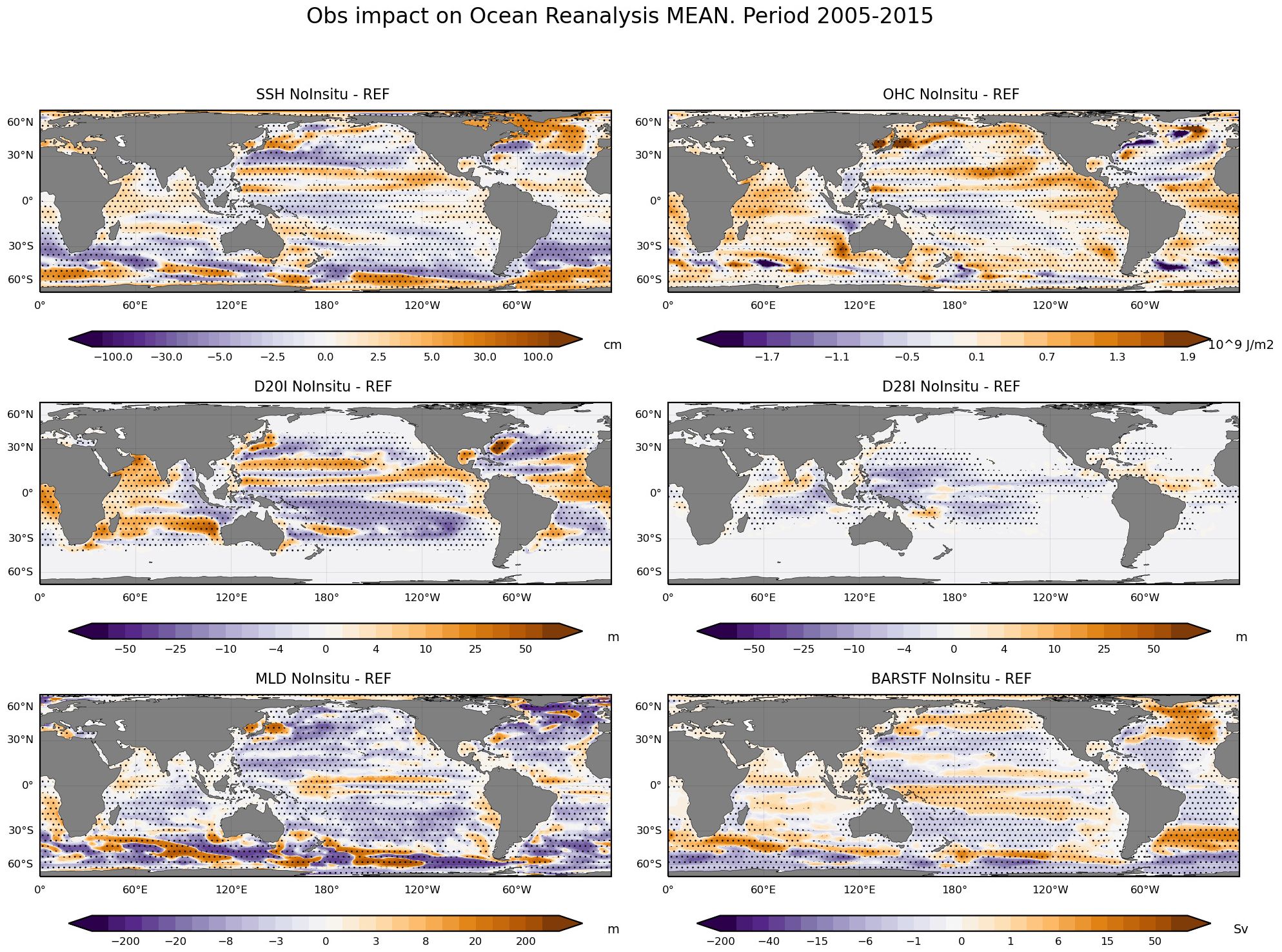
Figure 1. Impact of removing all in-situ ocean observations on the 2005-2015 mean state of the ocean initial conditions, as measured by the differences between experiments NoInsitu – REF. Shown are differences in SSH, OHC, D20I, D28I, MLD and barotropic stream function (BARSTF). Dotted areas indicate where the differences are significant at the 90% level.

The impact of removing Argo on the ocean mean state (Supplementary Figure S3) is broadly similar to removing all in-situ, which suggests the profound impact of Argo on the large-scale ocean state and circulation. This is especially true for the mid latitudes and the whole Atlantic basin. There are visible changes in the Atlantic barotropic circulation, which seem to be mostly due to Argo: removing the observations induces an increase of the anticyclonic gyre in the North and south Atlantic poleward of 30°, as well as a weakening of the subtropical gyres. There are also circulation changes along the paths of the main boundary current systems as well as the Equatorial Pacific. The impact of Argo in Western tropical Pacific differs from that of all in-situ, with visible differences over the warm pool (removing Argo produces shallowing of D28I only on the northern part), and the OHC/D20I/SSH, which do not show as stronger cooling/shallowing/decrease as when removing all in-situ. The impact of removing all in-situ in the Atlantic is confined to the Atlantic basin, with patterns similar to those in NoInsitu over the Atlantic (not shown).

The overall reduction of MLD in ORA-NoInsitu and ORA-NoArgo is likely to arise from the strong relaxation to SST, which tries to warm the ocean surface at a faster rate than the vertical ocean mixing spreads it in the vertical, thus leading to strong stratification, shallower mixed layers and reduced ocean heat uptake. In the reference experiments, the SST relaxation is aided by the in-situ observations in the vertical distribution of heat. This is confirmed in Supplementary Figure S4, which shows timeseries of the globally averaged accumulated heat flux from the SST relaxation and the ocean heat content in the different experiments. This implies that the in-situ observations have a strong impact on the estimations of heat absorption from ocean reanalyzes. The ocean observations also have an impact on the estimation of the mean SSH, which points towards the complementary role of in-situ and altimeter observations, casting doubts on whether the assimilation of sea level information from altimeter would be possible without the in-situ observations constraining the vertical ocean structure.

The removal of ocean observations has also an impact on the estimation of linear trends in ocean reanalysis, as can be seen in Figure 2. Removing all in-situ observations results in stronger deepening the thermocline in the Western Tropical Pacific, Northern Indian Ocean and Tropical Atlantic, which results in heat accumulation in the upper ocean, and deepening of the tropical warm pools. As with the mean state, removing the observations (either all or only Argo, not shown) leads to strong trends on the North Atlantic barotropic stream function, with a tendency towards weaker subtropical gyres and enhanced anticyclonic trend between 30N-50N, which also has a signature on upper ocean heat content tendency. There is also a visible impact on the shallowing of the mixed layer. The combined contribution of changes in stratification and circulation trends result in changes in the trends of SSH.

Figure 2

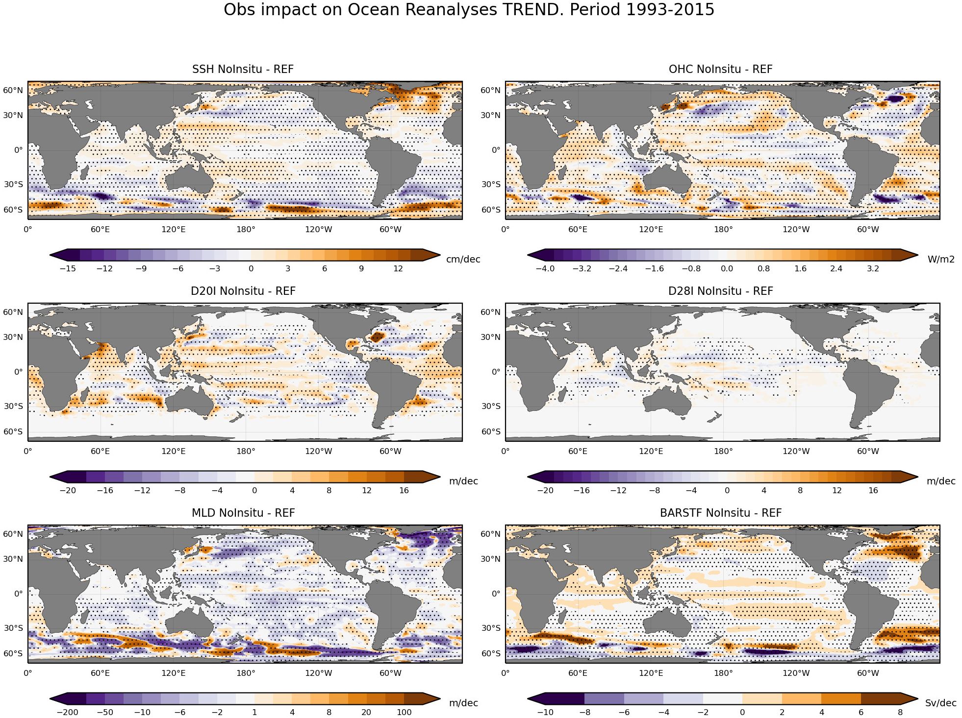
Figure 2. As Figure 1 but for the impact on linear trends, and for the period 1993-2015.

3.2 Observation impact on seasonal forecasts

3.2.1 Ocean variables

The analysis in this section aims at characterizing how ocean observations impact the seasonal forecasts of ocean variables. Figure 3 shows the impact in ocean mean state when forecasts are initialized in May (top plate) and November (bottom plate). The left column of each plate shows the differences in the initial conditions of SST, OHC and MLD, the middle and right columns show the impact in the forecast one and two seasons ahead respectively. (For the purposes of this plot, we take the monthly mean of the corresponding ORA one month prior to the forecast initialization to represent the initial condition). The most noticeable feature is the growth with lead time of an equatorial cold/warm SST bias over the Eastern Pacific/Atlantic. This growth is stronger in the forecast initialized in May. The cold SST pattern along the Equatorial Pacific is already visible in the first forecast month, as reported by Wei et al. (2023), which continues growing with lead time. The mid-latitudes exhibit a seasonal response: the wide-spread weak initial cold perturbation in SST amplifies in the winter hemisphere, but largely disappears over the summer hemisphere. Over the Atlantic basin, the observations also impact the mean SST over the gyres, which also grows with lead time. Contrary to the SST, the OHC forecast differences largely resemble the initial perturbation, as expected from the large thermal inertia of the ocean; but in the Equatorial Pacific there is an obvious eastward propagation of the initial perturbation anomaly. The MLD initial perturbation has different behavior: it seems to decrease with forecast lead time, and largely disappears over the summer hemisphere.

Figure 3

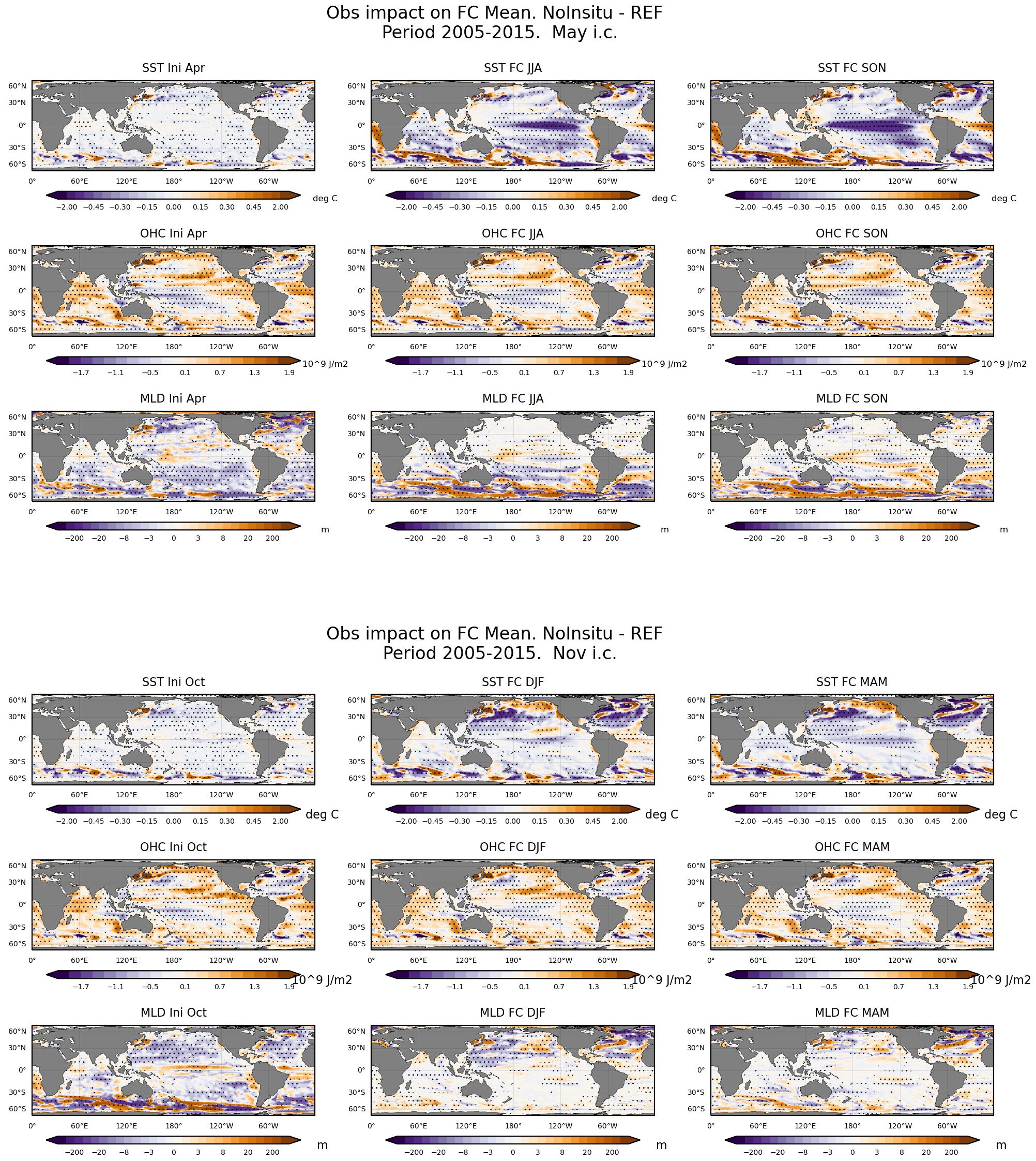
Figure 3. Impact of in-situ ocean observations in the mean state of seasonal forecasts of SST, OHC and MLD as measured by the experiments NoInsitu – REF (top/middle/lower rows of each individual plate). Shown are the results for forecasts initialized in May (top plate) and November (bottom plate). The differences in the initial conditions are shown in the left column, and the forecasts for the first and second seasons are in the central and rightmost columns respectively. The dotted areas indicate where the differences are significant at the 90% significant level.

The impact of Argo and Atlantic in-situ in the forecasts of ocean variables is shown in Supplementary Figures S5, S6 respectively. The evolution of initial conditions differences in these experiments also shows rapid local and seasonal dependent growth/decay of SST/mixed layer perturbation, and slower growth of SST forecasts differences associated with differences in OHC at initial time, which in the Equatorial Pacific are non-local. Removing the in situ observations in the Atlantic basin has a significant and lasting impact on the forecast of ocean variables in the whole basin, which for SST forecasts manifest on a characteristic pattern of warm equator, colder subtropical gyres and warmer subpolar gyre forecasts initialized in November. The in-situ observations in the Atlantic also seem to have some remote impact on other basins, an aspect that we will be discussed further below.

To gain insight on how the SST forecast uncertainty/error grows in the tropics we conduct a multivariate correlation analysis (local and non-local) for forecasts initialized in May, when the perturbations seem to grow more. Figure 4 shows the averaged local correlation between the SST in δFc at different lead times with δIni in different variables over the Equator (5S-5N, top) and at dateline (bottom) for May starts (see Supplementary Figure S7 for November starts). In the first month, the forecast SST are correlated with the initial SST and MLD. This correlation largely disappears in the second month, except for the winter hemisphere, where it lasts for until the next spring. A weak local correlation also remains in the Eastern Equatorial Pacific. Contrary to this decaying behavior, in the Equatorial band, the correlation between δFc(SST) and δIni(OHC) grows with time, both in amplitude and spatial extension, being negligible in the first month and most intense in the second season.

Figure 4

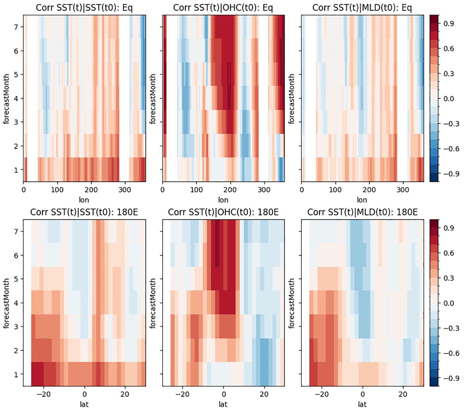
Figure 4. Local correlation between the SST in δFc at different lead times with δIni in different variables averaged over the Equator (top) and at the date line for forecasts initialized in May. The local correlation has been averaged over 5S-5N (top) and over all the longitudes (bottom).

The non-local relationship between initial and forecast perturbations is further explored via a simultaneous multivariate singular value decomposition (SVD) of the cross covariance matrix between δIni (SST,OHC,D28I,MLD) and δFc(SST) in the first month, first and second seasons. Here we present the results from forecast initialized in May, when the initial perturbations grow more over the tropical Pacific. This yields 2 dominant modes (Figure 5), with correlation of.98 and.89, explaining 45.1% and 11.3% of δFc(SST) (31.4% and 4.4% of δIni). The first mode (SVD1) is clearly associated with impacts in the low frequency variability arising from the changes in the observing system (Supplementary Figure S8), with very clear transitions corresponding to samples from the different pairs of OSES. The patterns are consistent with those of the impact on the mean state of the forecasts in Figure 3, where there is a growing cold/warm signal along the Equatorial Pacific/Atlantic Ocean, associated with an east-west dipole in OHC in the Pacific and positive OHC in the Atlantic. Interestingly, there seems to be a relation with shallower Pacific warm pool (-ve values of D28I) in the far western Pacific. The second mode (SVD2), with less explained variance, is associated with the interannual variability and trends of SST, with the final perturbation displaying a westward propagating SST anomaly which originates near the South American coast. This is associated with small initial uncertainty in SST confined in the Equatorial Eastern Pacific, and a hint of initial westward shift of the warm pool (increased D28I and MLD around the dateline).

Figure 5

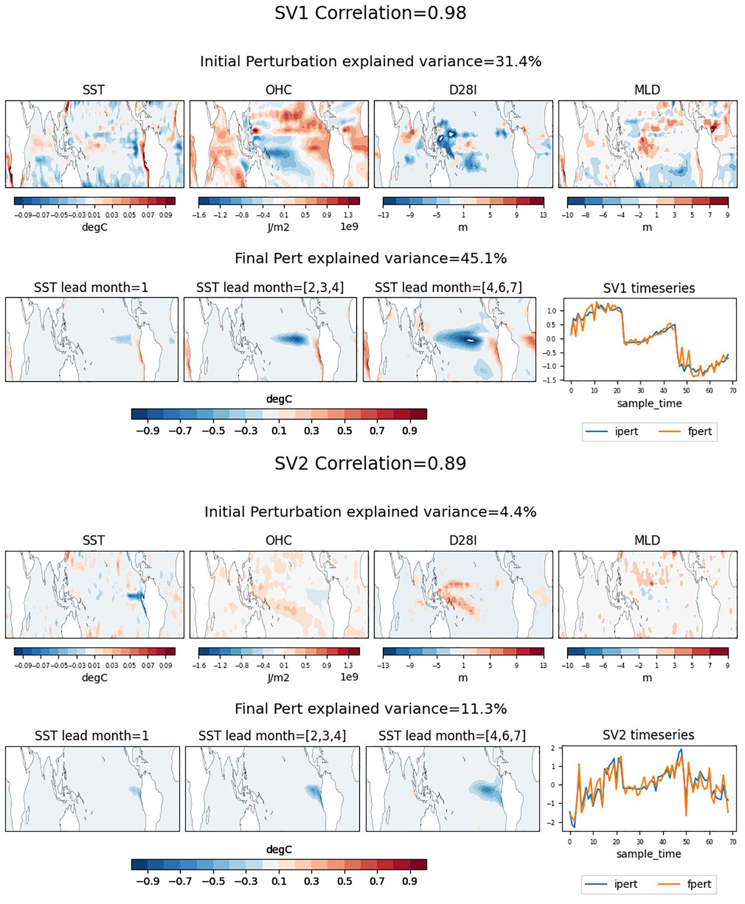
Figure 5. 1^st (top plate) and 2^nd (bottom plate) modes of the singular value decomposition between δIni (SST,OHC,D28I,MLD) and δFc(SST) in the first month, first and second seasons, for forecasts initialized in May. The perturbations are from the experiment pairs (NoInsitu-REF, NoArgo-REF, NoArgo-NoInsitu). Each plate shows the spatial structure of the initial/final perturbations (top/bottom rows) and the associated timeseries, for which the sample time (1-69) corresponds the different pairs of perturbations: NoInsitu-REF (1-23), NoArgo-REF (24-46) and NoArgo-NoInsitu (47-69).

The non-local relationship between the observing system in the Atlantic basin and the forecasts of SST in the tropical area, i.e. the analysis including the pair NoInsAtl-REF, yields only one pair with sizeable correlations (.73), explaining 15.7% and 11.9% of the variance in δFc and δIni respectively (Figure 6). Although the total variance is modest, the spatial patterns are meaningful, indicating a remote influence between the initial conditions if the Tropical Atlantic in the seasonal forecast of SST over the Eastern Indian Ocean, as well as a local impact on the forecast of SST in the Tropical Atlantic. In particular, negative perturbations of OHC and D28I in the Equatorial Atlantic manifest on negative local SST anomalies in the first season of the forecast. In the second season, these local anomalies grow, and remote anomalies in the Eastern Indian Ocean of opposite sign emerge, likely mediated via the atmospheric bridge. This direct response, which does not involve the tropical Pacific as mediator, is consistent with the direct Matsuno-Gill response described by Kucharski et al. (2009).

Figure 6

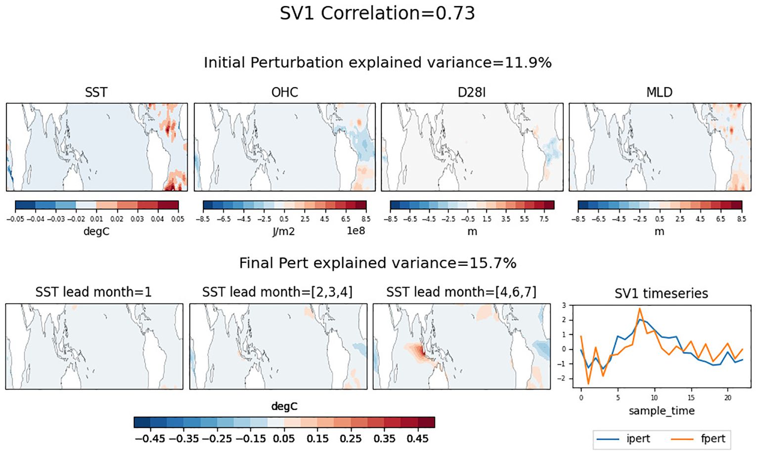
Figure 6. 1^st mode of the singular value decomposition for pair NoInsAtl-REF between δIni (SST,OHC,D28I,MLD) and δFc(SST) in the first month, first and second seasons, for forecasts initialized in May. Each plate shows the spatial structure of the initial/final perturbations (top/bottom rows) and the associated timeseries..

We now return to the main perturbation analysis using the 3-pairs of experiment and investigate the impact of the ocean observing system with the long term trends in the forecasts. It has been reported that errors in seasonal forecasts of SST trends are common to several forecast models (L’Heureux et al., 2022), and that the misrepresentation of trends in seasonal forecasts can degrade the ENSO prediction skill, especially for forecasts initialized in May (Balmaseda et al., 2024), when the forecasts overestimate the warming trends over the Equatorial Pacific (their Figure 6). Figure 7 shows the contribution of all in-situ and Argo Ocean observations to the representation of linear trends (1993-2015) in seasonal forecasts initialized in May. Removing the in-situ and Argo observations leads to cooler trends in the seasonal forecasts, which would reduce the errors. For instance, the SST Nino3.4 trends are (0.5, 0.2, 0.3) deg/decade in (REF, NoInsitu, NoArgo), while they are insignificant in the observations. We note that the spatial patterns of the trends in the initial conditions in Figure 2 resemble those of the SVD2 mode of the main perturbation analysis in Figure 5, suggesting that small changes in trends of the zonal gradient of OHC (warmer west-colder east) and deeper and westward shift of the warm pool in NoInsitu are associated with the colder SST forecast trends. To quantify the pattern similarity, we compute the correlation between the NoInsitu-REF initial conditions trend difference with the SVD. The pattern correlation with the SVD2 mode is (0.8,0.7,0.6,0.7) for (SST,OHC,D28I,MLD), while the corresponding correlations with SVD1 are much lower (0.3,0.3,0.3,0.3). The NoArgo-REF initial conditions trends are equally correlated with SVD1 and SVD2. These results support the idea that changes in the observing system can lead to spurious trends in the seasonal forecast. In The tropical Pacific, changes in the structure of the warm pool, zonal gradients in the upper ocean heat content and the Equatorial upper ocean east of the Galapagos Islands appear associated with the developments of trends in the forecasts.

Figure 7

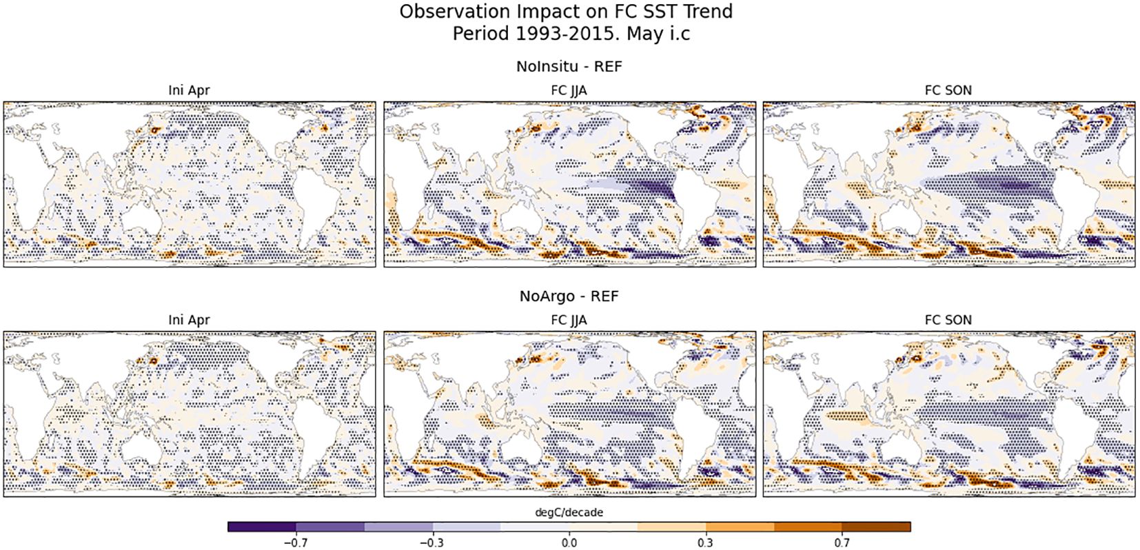
Figure 7. Impact of in-situ ocean (top) and Argo (bottom) observations in the linear trend of May starts seasonal forecasts of SST. The differences in the initial conditions are shown in the left column, and the forecasts for the first and second seasons are in the central and rightmost columns respectively. The dotted areas indicate where the differences are significant at the 90% significant level.

3.2.2 Atmospheric variables

We now look at the impact of the ocean observations in forecasts of atmospheric variables. Figure 8 shows the 2005-2015 mean difference NoInsitu-REF of seasonal forecasts initialized in May for the 1^st and 2^nd seasons into the forecasts. (See Supplementary Figure S9 and left column of Figure 9 for November starts). The impact on T2m largely resembles the pattern of SST, but we also see differences over land, with colder values visible especially over the northern winter in large parts of North America and Eurasia. There are also significant impacts in tropical precipitation which are physically consistent with the changes in SST in Figure 3: stronger Equatorial Pacific cold tongue and shallower warm pools lead to drier conditions over the Equator, Western Pacific and poleward migration of the Intertropical Convergence Zone (ITCZ). In contrast, there is increased precipitation over Atlantic, Amazone and Caribbean (consistent in warmer conditions there). There are significant changes on the large-scale atmospheric circulation. The zonal winds at lower levels (U850) show strengthening of the Equatorial easterlies, especially for forecasts initialized in May, a signature of the Bjerkness feedback, which would contribute to the strengthening of the equatorial cold bias. There is also a large-scale significant change on the distribution of MSL, with higher values over the Pacific and lower values over the Atlantic, consistent with the SST differences and more visible in the forecasts initialized in May. Outside of the tropics there are also visible changes in the atmospheric circulation, especially in the winter season, with shifts in the lower-level jets at mid latitudes and associated changes in MSL, as well as changes in the precipitation patterns along the Atlantic storm track.

Figure 8

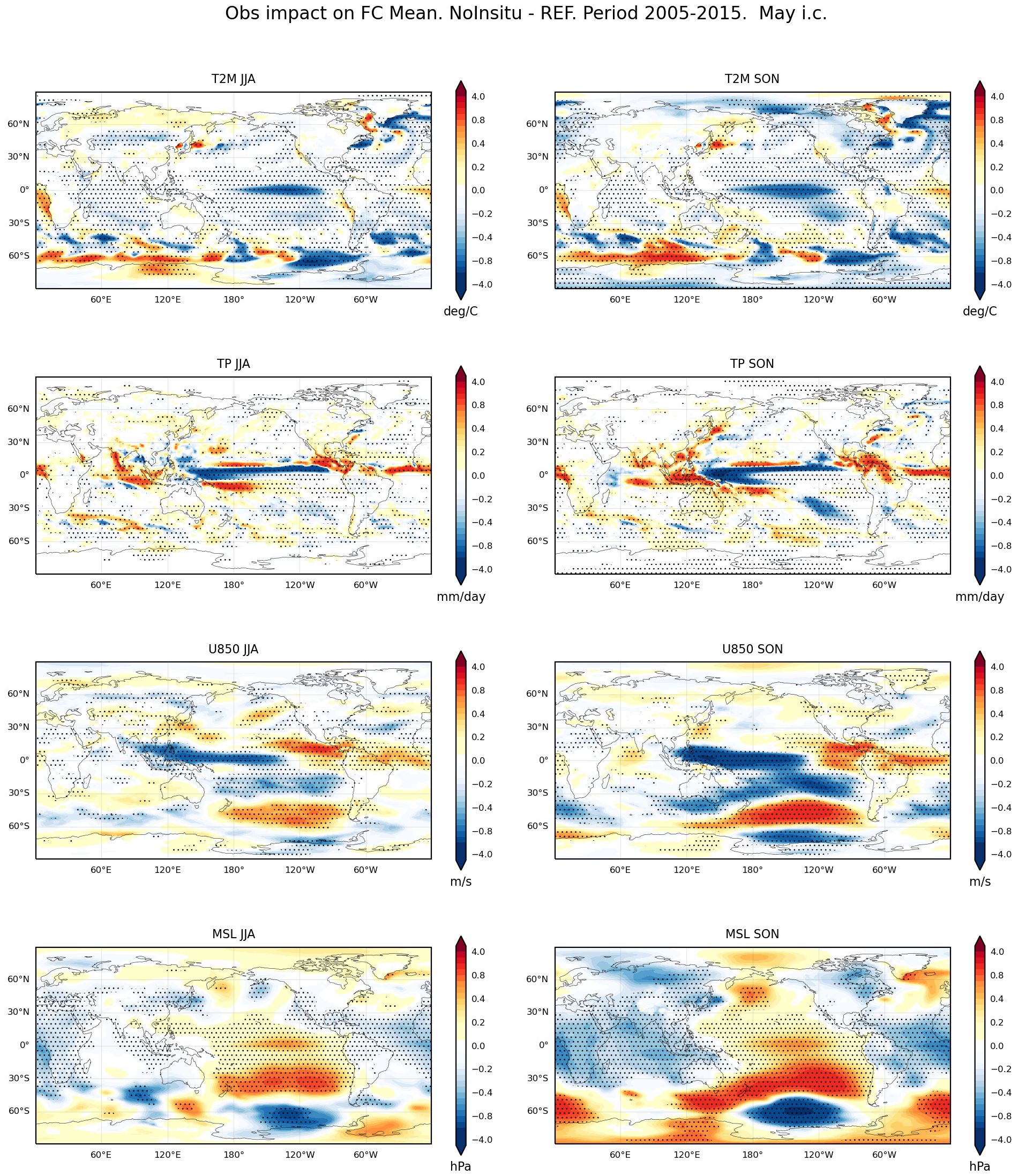
Figure 8. Impact of in-situ ocean observations in the 2005-2015 mean state of seasonal forecasts of atmospheric variables as measured by the differences between experiments NoInsitu and REF. shown are forecasts are initialized in May for the first and second seasons into the forecasts (left and right panels in the individual plates). The different rows correspond to different variables T2m, total precipitation (TP), U850 and mean sea level pressure (MSL). The dotted areas indicate that the differences in the mean are significant at the 90% level.

Figure 9

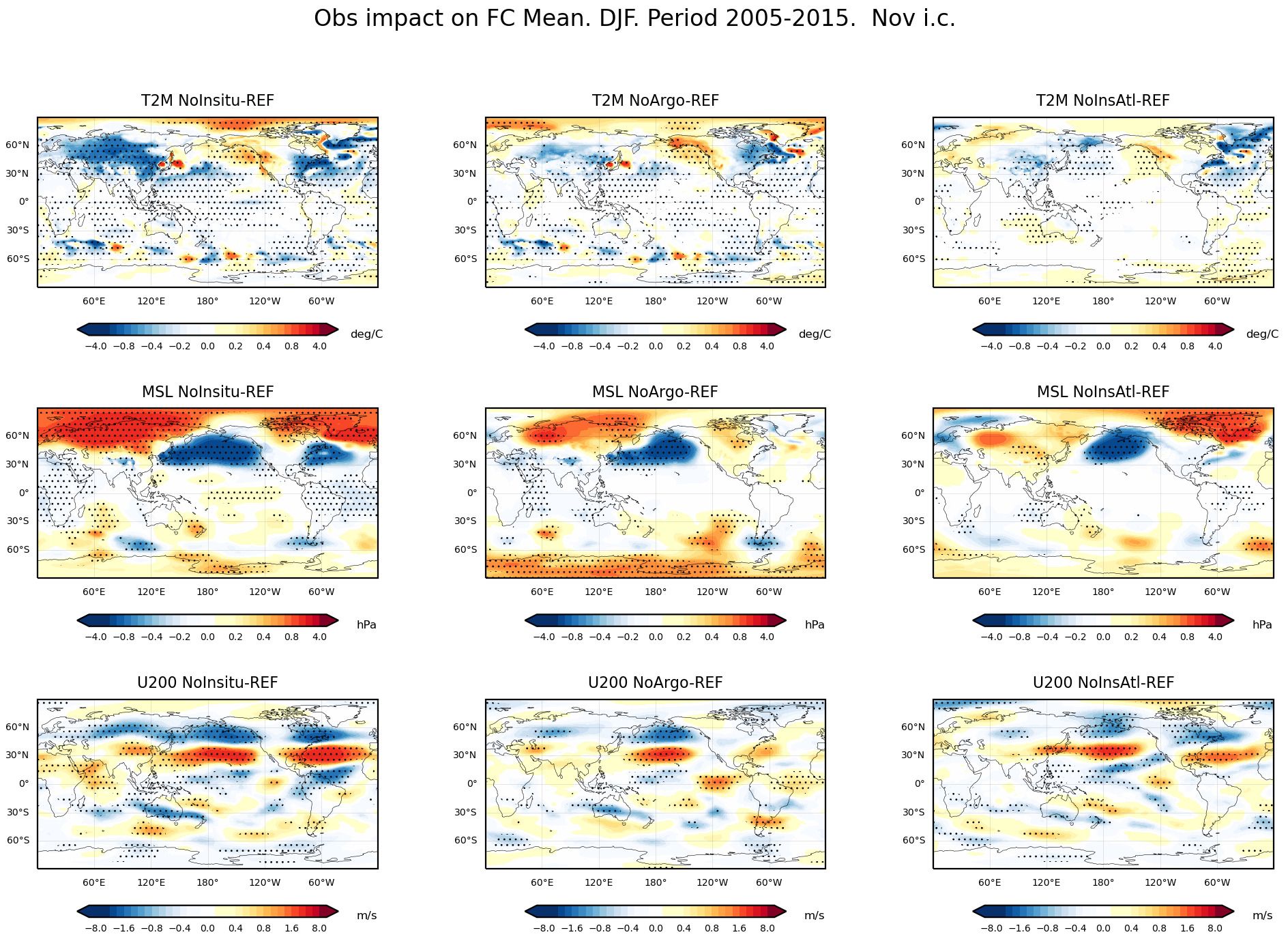
Figure 9. Impact of ocean observations in the 2005-2015 mean state of seasonal forecasts of atmospheric variables as measured by the differences between experiments NoInsitu- REF, NoArgo-REF and NoInsAtl-REF (left, middle and right column of each plate). Shown are forecasts are initialized in November for the first season into the forecast. The different rows correspond to different variables T2m, mean sea level pressure (MSL) and zonal wind at 200hPa (U200). The dotted areas indicate that the differences in the mean are significant at the 90% level.

Figure 9 shows the comparison of the impact on the atmospheric mean state between the different FC-OSES, this time for the first season into the forecasts. Shown are the differences between NoInsitu-REF (left), NoArgo-REF (middle) and NoInsAtl-REF (right) for forecasts initialized in November. The impact in T2m over the oceans is mostly local: in NoArgo it resembles that of NoInsitu, but is overall weaker, and confined within the Atlantic basin in NoInsAtl. However, the impact on atmospheric circulation is nonlocal, consistent the atmosphere responding to large scale temperature gradients, and the tropical convection linked to the structure of the warm pools, affecting the global circulation. Removing the in-situ ocean observations in the Atlantic leads to changes in MSL in other basins and at polar latitudes, and, interestingly, during the boreal winter the Aleutian Low is intensified in all three experiments NoInsitu, NoArgo and NoInsAtl. The upper-level circulation (U200) shows significant changes in the position of the jets, both in winter and summer. These results highlight the importance of representing correctly the large-scale SST gradients, for which a uniform observational coverage is required.

The impact of observations on the forecast trends (1993-2015) of atmospheric variables is displayed in Figure 10 for May starts. Over the ocean, T2m trends are similar to those in SST in Figure 7, and in the second season, they affect significantly some land areas, with colder values over Australia, Eastern part of North America, Central Europe and warmer values over Eastern Siberia. They also affect the forecasts of tropical precipitation trends across the basins, and the forecasts of the large-scale tropical circulation, leading to patterns that resemble cold La Nina conditions.

Figure 10

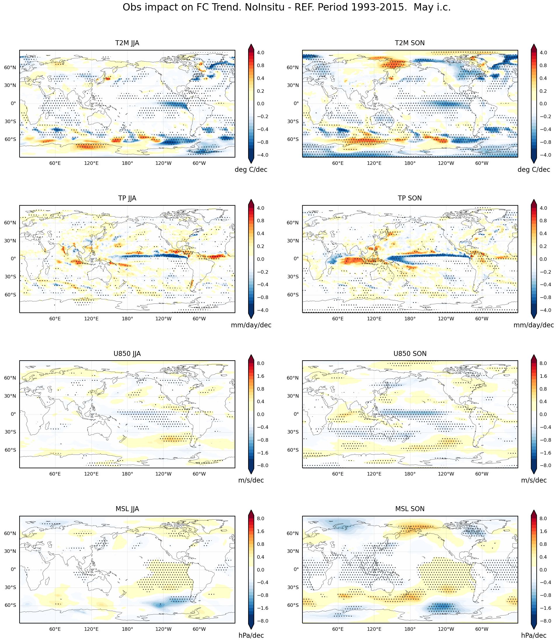
Figure 10. Differences (NoInsitu – REF) in linear trends (1993-2015) of atmospheric variables in seasonal forecasts initialized in May. Shown are the forecasts for the 1^st and 2^nd seasons (left and right columns). Dotted areas indicate that the differences are significant at the 90% level.

4 Summary and conclusions

A series of ocean reanalyzes and seasonal reforecast observing system experiments has been conducted to characterize the impact of in-situ ocean observations on estimation of the ocean state used to initialize seasonal forecasts, as well as their impact on the mean state and trends of the coupled forecasts of both ocean and atmospheric circulation.

The ocean observations have a profound impact on the mean state of the ocean circulation, its removal leading to i) changes in the heat content and gradients in the tropics (shallow thermocline and weaker zonal gradients in the Pacific, deeper thermocline in the Atlantic), ii) shallowing of the tropical warm pools, iii) widespread shallowing of the mixed layer (except for ocean deep convective regions), and iv) changes in the gyre circulation. In the Atlantic, this impact is dominated by the Argo observing system.

The impact of the observations is also visible in the mean state of seasonal forecasts. The shallower mixed layer impact is mostly local, leading to overall cooling of the SST. Although it decays with lead time, being short-lived in summer (about 1 month), at mid-latitudes persists during the whole winter season. The impact of the subsurface temperature gradients in the tropics is nonlocal and amplifies with lead time, being negligible in the first month and larger in the second season. This amplification seems associated with a positive coupled feedback, and there are suggestions that the structure of the warm pools may play a role, either independently or in connection with a coupled growing mode. Specifically, removing in-situ observations leads to colder Western Pacific in the initial conditions, which translates in colder SST along the Pacific in the forecasts. Changes are also visible in the forecasts of atmospheric circulation, affecting the structure of overall Walker circulation in the tropics, with visible changes in the trade winds, mean sea-level pressure and tropical precipitation, consistent with the existence of a coupled feedback. There are also changes at mid-latitudes, producing colder T2m in the boreal winter over large parts of North America and Eurasia, changes in the precipitation along the storm tracks and modifications of the jet structure and mean sea level pressure. Some of these changes are visible even when the observations are withdrawn only in the Atlantic basin, highlighting the non-local nature of the atmospheric response.

The removal of the ocean observations also affects the estimation of the long-term linear trends in ocean initial conditions in a non-trivial manner, affecting the absorption and redistribution of heat in the ocean. It also affects the trends in the seasonal forecasts of both ocean and atmospheric circulation, which seems to occur via two different mechanisms: i) one of them is associated with progressive changes in the mean state, since the removal of ocean observations progressively induces colder SST along the Central Equatorial Pacific; ii) the second one is related with changes in the trends in the initial conditions, and this seems to be associated with colder Eastern Pacific and westward displacement of the warm pool.

The results presented indicate the importance of observations for initializing the mixed layer, the warm pools, and the large-scale gradients in the ocean subsurface, which are aspects contributing to mean state and variability of the seasonal forecasts. The large impact that the ocean observations have in the mean state and trends implies that for forecasting systems to benefit from the improvements of the observing system, it is important to reduce mean errors either via better models or explicit treatment of model bias, at least in the assimilation stage. The specific mechanisms are likely to be dependent on the forecasting and assimilation system. For instance, the shallowing of the mixed layer when removing ocean observations will depend on the way of assimilating SST. In the experiment presented here, the SST were constrained via simple nudging, and the initialization was conducted separately in ocean and atmosphere. The impact of observation may be different if the initialization is conducted in coupled data assimilation mode. It is expected that more sophisticated data assimilation methods (either in coupled or uncoupled data assimilation) should be able to spread the SST information in the vertical more efficiently. Therefore, it is desirable conducting coordinated OSEs in a multi-system framework. This is the idea behind the project SynObs (Fujii and Co-authors, 2024, this issue)¹, a recently launched initiative to evaluate observation impact in a coordinated manner. It is expected that these intercomparison efforts will come in time to provide feedback to the implementation of the Tropical Pacific Observing System (TPOS, Kessler et al., 2021), which is currently underway.

Data availability statement

The raw data supporting the conclusions of this article will be made available by the authors, without undue reservation.

Author contributions

MB: Conceptualization, Data curation, Formal analysis, Funding acquisition, Investigation, Methodology, Project administration, Resources, Software, Supervision, Validation, Visualization, Writing – original draft, Writing – review & editing. BB: Data curation, Investigation, Methodology, Validation, Writing – review & editing. MM: Formal analysis, Investigation, Methodology, Validation, Writing – review & editing. ST: Conceptualization, Investigation, Methodology, Project administration, Software, Supervision, Writing – review & editing. HZ: Data curation, Investigation, Methodology, Software, Writing – review & editing. FV: Supervision, Writing – review & editing. TS: Supervision, Writing – review & editing.

Funding

The author(s) declare financial support was received for the research, authorship, and/or publication of this article. This research was partially supported by the European Union H2020 projects AtlantOS (grant no. 633211), EuroSea (agreement no 862626) and by the Copernicus Marine Environment Monitoring Service’s GLORAN tender.

Conflict of interest

The authors declare that the research was conducted in the absence of any commercial or financial relationships that could be construed as a potential conflict of interest.

Publisher’s note

All claims expressed in this article are solely those of the authors and do not necessarily represent those of their affiliated organizations, or those of the publisher, the editors and the reviewers. Any product that may be evaluated in this article, or claim that may be made by its manufacturer, is not guaranteed or endorsed by the publisher.

Supplementary material

The Supplementary Material for this article can be found online at: https://www.frontiersin.org/articles/10.3389/fmars.2024.1456013/full#supplementary-material

Footnotes

1. ^ Fujii, Y. and Co-authors (2024). The international multi-system OSEs/OSSEs by the UN Ocean Decade Project SynObs and its early results. Front. Mar. Sci. This issue (submitted).

References

Balan-Sarojini B., Balmaseda B. M., Vitart F., Roberts C., Zuo H., Tietsche S., et al. (2024). Impact of ocean in-situ observations in subseasonal forecasts. Front. Mar. Sci. 11. doi: 10.3389/fmars.2024.1396491

Crossref Full Text | Google Scholar

Balmaseda M. A. (2017). Data assimilation for Initialization of seasonal forecasts. 2017. The Sea: The Science of Ocean Prediction. J. Mar. Res. 75, 331–359. doi: 10.1357/002224017821836806

Crossref Full Text | Google Scholar

Balmaseda M., Anderson D. (2009). Impact of initialization strategies and observations on seasonal forecast skill. Geophys. Res. Lett. 36, L01701. doi: 10.1029/2008GL035561

Crossref Full Text | Google Scholar

Balmaseda M. A., Davey M. K., Anderson D. L. T. (1995). Decadal and seasonal dependence of ENSO prediction skill. J. Climate 8, 2705–2715. doi: 10.1175/1520-0442(1995)008<2705:DASDOE>2.0.CO;2

Crossref Full Text | Google Scholar

Balmaseda M. A., Fujii Y., Alves O., Awaji T., Behringer D., Ferry N., et al. (2010). “Initialization for seasonal and decadal forecasts,” in Proceedings of OceanObs’09: Sustained Ocean Observations and Information for Society, vol. Vol. 2 . Eds. Hall J., Harrison D. E., Stammer D. (ESA Publication WPP-306, Venice), 19–26. doi: 10.5270/OceanObs09.cwp.02

Crossref Full Text | Google Scholar

Balmaseda M. A., McAdam R., Masina S., Michael M., Senan R., de Bosisséson E., et al. (2024). Skill assessment of seasonal forecasts of ocean variables. Front. Mar. Sci. 11. doi: 10.3389/fmars.2024.1380545

Crossref Full Text | Google Scholar

Dee D. P., co-authors (2011). The ERA-Interim reanalysis: configuration and performance of the data assimilation system. Q. J. R. Meteor. Soc 137, 553–597. doi: 10.1002/qj.828

Crossref Full Text | Google Scholar

Du D., Subramanian A. C., Han W., Wei H. H., Sarojini B. B., Balmaseda M., et al. (2023). Assessing the impact of ocean in situ observations on MJO propagation across the maritime continent in ECMWF subseasonal forecasts. J. Adv. Modeling. Earth Syst. 15, e2022MS003044. doi: 10.1029/2022MS003044

Crossref Full Text | Google Scholar

Folland C. K., Colman A. W., Rowell D. P., Davey M. K. (2001). Predictability of northeast Brazil rainfall and real-time forecast skill 1987–98. J. Clim. 14, 1937–1958. doi: 10.1175/1520-0442(2001)014<1937:PONBRA>2.0.CO;2

Crossref Full Text | Google Scholar

Fujii Y., co-authors (2019). Observing system evaluation based on ocean data assimilation and prediction systems: on-going challenges and future vision for designing/supporting ocean observational networks. Front. Mar. Sci. 6. doi: 10.3389/fmars.2019.00417

PubMed Abstract | Crossref Full Text | Google Scholar

Fujii Y., Cummings J., Xue Y., Schiller A., Lee T., Balmaseda M. A., et al. (2015). Evaluation of the Tropical Pacific Observing System from the ocean data assimilation perspective. Q. J. R. Meteorol. Soc. 141, 2481–2496. doi: 10.1002/qj.2579

Crossref Full Text | Google Scholar

Fujii Y., Kamachi M., Nakaegawa T., Yasuda T., Yamanaka G., Toyoda T., et al. (2011). “Assimilating ocean observation data for ENSO monitoring and forecasting,” in Climate variability - Some Aspects, Challenges and Prospects. Ed. Hannachi A. (InTech Open, Rijeka), 75–98. doi: 10.5772/30330

Crossref Full Text | Google Scholar

Giannini A., Saravanan R., Chang P. (2003). Oceanic forcing of Sahel rainfall on interannual to interdecadal timescales. Science 302, 1027–1030. doi: 10.1126/science.1089357

PubMed Abstract | Crossref Full Text | Google Scholar

Goddard L., Dilley M. (2005). El niño: catastrophe or opportunity. J. Clim. 18, 651–665. doi: 10.1175/JCLI-3277.1

Crossref Full Text | Google Scholar

Goddard L., Graham N. E. (1999). The importance of the Indian Ocean for simulating precipitation anomalies over Eastern and Southern Africa. J. Geophys. Res. 104, 19099–19116. doi: 10.1029/1999JD900326

Crossref Full Text | Google Scholar

Good S. A., Martin M. J., Rayner N. A. (2013). EN4: Quality controlled ocean temperature and salinity profiles and monthly objective analyses with uncertainty estimates. J. Geophys. Res.-Ocean. 118, 6704–6716. doi: 10.1002/2013JC009067

Crossref Full Text | Google Scholar

GOOS (2018). Global Ocean Observing System - Climate. Available online at: http://www.goosocean.org/index.php?option=com_content&view=article&id=3&Itemid=103 (Accessed October 24, 2018).

Google Scholar

Gouretski V., Reseghetti F. (2010). On depth and temperature biases in bathythermograph data. Development of a new correction scheme based on analysis of a global ocean database. Deep-Sea. Res. Pt. I. 57, 812–833. doi: 10.1016/j.dsr.2010.03.011

Crossref Full Text | Google Scholar

Huang B., Shin C.-S., Shukla J., Marx L., Balmaseda M., Halder S., et al. (2017). Reforecasting the ENSO events in the past 57 years, (1958-2014). J. Climate 30, 7669–7693. doi: 10.1175/JCLI-D-16-0642.1

Crossref Full Text | Google Scholar

Johnson S., Stockdale T., Ferranti L., Balmaseda M., Molteni F., Magnusson L., et al. (2019). ECMWF-SEAS5: the new ECMWF seasonal forecast system. Geosci. Model. Develop. Geosci. Model. Dev. 12, 1087–1117. doi: 10.5194/gmd-12-1087-2019

Crossref Full Text | Google Scholar

Kessler W., Cravatte S., Co-authors (2021). Final Report TPOS 2020. Available at: https://tropicalpacific.org/wp-content/uploads/2021/08/TPOS2020-Final-Report-2021.08.23.pdf (accessed on 2nd Sept 2024).

Google Scholar

Kucharski F., Bracco A., Yoo J. H., Tompkins A., Feudale L., Ruti P., et al. (2009). A Gill-Matsuno-type mechanism explains the tropical Atlantic influence on African and Indian monsoon rainfall. Quart. J. R. Meteor. Soc. 135, 569–579. doi: 10.1002/qj.406

Crossref Full Text | Google Scholar

Kumar A., Chen M., Xue Y. (2015). An analysis of the temporal evolution of ENSO prediction skill in the context of the equatorial Pacific Ocean Observing System. Mon. Wea. Rev. 143, 3204–3213. doi: 10.1175/MWR-D-15-0035.1

Crossref Full Text | Google Scholar

L’Heureux M., Tippett M. K., Wang W. (2022). Prediction Challenges from errors in tropical pacific sea surface temperature trends. Front. Clim. 4. doi: 10.3389/fclim.2022.837483

Crossref Full Text | Google Scholar

McPhaden M. J., Lee T., Fournier S., Balmaseda M. A. (2020). “ENSO observations,” in “El Niño Southern Oscillation in a Changing Climate”. Eds. McPhaden M. J., Santoso A., Cai W. (American Geophysical Union). doi: 10.1002/9781119548164.ch3

Crossref Full Text | Google Scholar

Moltman T., co-authors (2019). A global ocean observing system (GOOS), delivered through enhanced collaboration across regions, communities, and new technologies. Front. Mar. Sci. 6. doi: 10.3389/fmars.2019.00291

Crossref Full Text | Google Scholar

Palmer T. N., Anderson D. L. T. (1994). The prospects for seasonal forecasting—A review paper. Q.J.R. Meteorol. Soc 120, 755–793. doi: 10.1002/qj.49712051802

Crossref Full Text | Google Scholar

Rodwell M., Folland C. K. (2002). Atlantic air–sea interaction and seasonal predictability. Q. J.Roy. Meteorol. Soc 128, 1413–1443. doi: 10.1002/qj.200212858302

Crossref Full Text | Google Scholar

Roenmich D., co-authors (2019). On the future of argo: A global, full-depth, multi-disciplinary array. Front. Mar. Sci. 6. doi: 10.3389/fmars.2019.00439

Crossref Full Text | Google Scholar

Saji N. H., Goswami B. N., Vinayachandran P. N., Yamagata T. (1999). A dipole mode in the tropical Indian Ocean. Nature 401, 360–363. doi: 10.1038/43854

PubMed Abstract | Crossref Full Text | Google Scholar

Torrence C., Webster P. J. (1998). The annual cycle of persistence in the El Niño-Southern Oscillation. Q. J. R. Meteorol. Soc 124, 1985–2004. doi: 10.1256/smsqj.55009

Crossref Full Text | Google Scholar

Wei H. H., Subramanian A. C., Karnauskas K. B., Du D., Balmaseda M. A., Sarojini B. B., et al. (2023). The role of in situ ocean data assimilation in ECMWF subseasonal forecasts of sea-surface temperature and mixed-layer depth over the tropical Pacific ocean. Q. J. R. Meteorol. Soc. 149, 3513–3524. doi: 10.1002/qj.4570

Crossref Full Text | Google Scholar

Xue Y., Wen C., Yang X., Behringer D., Kumar A., Vecchi G., et al. (2017). Evaluation of tropical Pacific observing system using NCEP and GFDL ocean data assimilation systems. Clim. Dyn. 49, 843–868. doi: 10.1007/s00382-015-2743-6

Crossref Full Text | Google Scholar

Zuo H., Balmaseda M. A., Tietsche S., Mogensen K., Mayer M. (2019). The ECMWF operational ensemble reanalysis–analysis system for ocean and sea ice: a description of the system and assessment. Ocean. Sci. 15, 779–808. doi: 10.5194/os-15-779-2019

Crossref Full Text | Google Scholar