Tensor adaptive reconstruction cascaded with spatial-spectral fusion for marine target detection

Hyperspectral target detection has a wide range of applications in marine target monitoring. Traditional methods for target detection take less consideration of the inherent structural information of hyperspectral images and make insufficient use of spatial information. These algorithms may experience degradation in efficacy during complex scenarios. To address these issues, this study introduces a hyperspectral target detection approach based on tensor adaptive reconstruction cascade spatial-spectral fusion, named as TRSSF. First, the position of the pixel that best matches the prior spectrum is obtained. Second, tensor decomposition and reconstruction of the original hyperspectral data are performed. Linear total variation smoothing is used to acquire the principal components in the spatial dimensionality unfolding of data, and correlation regularization robust principal component analysis is employed to derive the spectral dimensionality unfolding’s principal components of data. Finally, the spatial-spectral fusion method is proposed for detecting hyperspectral targets on the reconstructed data. The use of multi-morphological feature fusion can fully utilize the spatial features to complement the spectral detection results and improve the integrity of target detection. The experiments conducted on the publicly available dataset and collected datasets demonstrated the effective detection achieved by the proposed method.

1 Introduction

The transport, distribution, and accumulation of marine targets, such as oil pollution and wake (as shown in Figure 1), have a significant detrimental effect on marine ecosystems. Hyperspectral imaging (HSI) offers the advantage of abundant spectral information, enabling the differentiation of marine targets of similar shapes and sizes but varying materials (Zou and Shi, 2015; Sun et al., 2024a). As hyperspectral remote sensing has advanced, hyperspectral image super-resolution (Li et al., 2022a, 2023a, b, 2024) and target detection technology have become increasingly important. Of these, target detection technology has found extensive applications in civilian and military domains (Nasrabadi, 2013; Hou et al., 2022; Wang et al., 2024). In the civilian field, the technology can be used in plant disease detection, insect pest detection, mineral detection, medical detection, etc. In the military field, it can be used in landmine detection, sea target detection, and ground camouflage hidden target detection (Coorey, 2018; Wang et al., 2023).

Figure 1

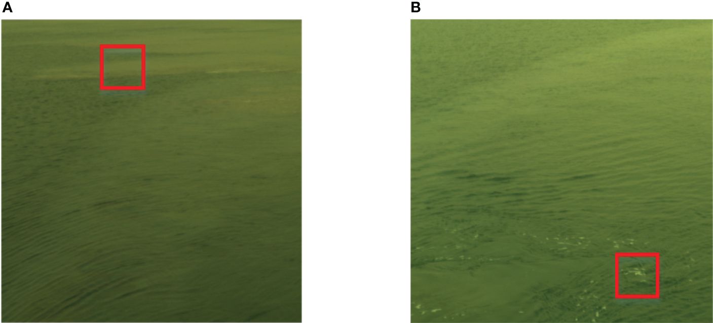
Figure 1. Water surface oil pollution (A) and wake (B).

As hyperspectral technology has progressed, numerous traditional strategies for hyperspectral imagery target detection have long been formed (Chen et al., 2011; Li and Du, 2016; Liu et al., 2021a). Hyperspectral target detection methods are categorized based on the amount of information fed into spectral-based, spatial-spectral, and deep feature extraction methods (Du and Zhang, 2010; Zhao et al., 2020c; Hou et al., 2021; Gao et al., 2023). Numerous hyperspectral target detection approaches rely on spectral domain data. The constrained energy minimization (CEM) technique devises a filter capable of minimizing information output while adhering to constraints imposed by the prior target spectrum (Farrand and Harsanyi, 1997). Spectral angle mapper (Kruse et al., 1993) can detect the targets without information distribution assumptions and is considered one of the most straightforward detection mechanisms. Spectral matching filter (MF) (Manolakis et al., 2009) defines target detection as a hypothetical test and has good detection performance in a simple background. Orthogonal subspace projection is a subspace model detection algorithm in a linear mixed model (Harsanyi and Chang, 1994). Adaptive cosine estimation is a probability statistical algorithm that employs various techniques to extend detection statistics, improving the differentiation between the target and the background (Manolakis et al., 2003). Spectral information divergence calculates the information divergence between two spectrums (Chang, 1999). Lin et al. proposed a multi-target band selection method for hyperspectral target detection, based on an ideal solution optimization strategy (MOBS), with the aim of selecting bands with greater target separation and stronger robustness for different application scenarios (Sun et al., 2024b).

With the increase in spatial information in hyperspectral images, hyperspectral target detection methods that integrate spatial and spectral information have emerged (Wei et al., 2019). Yang and Shi (2016) proposed a method that uses a target pixel to execute target detection and total variation to smooth the space of an image. Zhao et al. (2021b) designed a fractional adaptive CEM. The initial data is processed with fractional Fourier, and then a locally CEM is used for target acquisition. Gao et al. introduced the tree-structured encoding approach to locate targets in hyperspectral data (Sun et al., 2020). Yang et al. introduced the sparse spatial constraint energy minimization (Yang et al., 2019; Zhao et al., 2020b). Sun et al. proposed an information entropy estimation target detection method based on point set topology. The method consists of constructing a parallel topological space to sort the raw HSI data and introducing information entropy estimation in combination with a priori information about the target (Sun et al., 2024c).

In the realm of adopting deep feature algorithms, Zhang et al. presented a hyperspectral target detection neural network, which uses deep features (Li and Du, 2016; Zhang et al., 2020). The novel deep spatial-spectral network was developed by Shi et al. as an unsupervised detection means. This network incorporates a typical detector and an edge-preserving filter to identify targets (Shi et al., 2020). Generally, traditional methods often overlook the inherent structural characteristics of hyperspectral data and underutilize spatial information. Dong et al. presented a lightweight convolutional neural network (LCNN) (Dong et al., 2023) for reducing computational complexity. In deep learning approaches, the limited samples pose challenges in training deep networks.

In recent years, some new methods of using tensors have attracted the interest of researchers. Tensor extends the concepts of vectors and matrices to accommodate higher-order data so that multidimensional datasets can be treated as a whole. Tensor representation can provide a convenient and accurate strategy for capturing the interrelationship between multiple dimensions (Kolda and Bader, 2009). HSI encompasses both spatial and spectral dimensions, thus is recognized as a third-order data cube (Zhao et al., 2021a). The tensor representation technique has found applications in various hyperspectral image processing tasks, such as the noise reduction algorithm (Renard and Bourennane, 2008; Guo et al., 2013; Liu et al., 2021b), unmixing algorithm (Veganzones et al., 2015), and classification algorithm (Renard and Bourennane, 2009).

There are few studies using the tensor representation method for hyperspectral target detection. Chen et al. introduced the technique called tensor principal component analysis through Fourier transform (TRPCAF), which considers the hyperspectrum, including principal components and residuals (Chen et al., 2018; Chen and Wang, 2019). Li et al. introduced the prior tensor approximation (PTA) technique to detect anomalies in hyperspectral images (Li et al., 2020; Feng et al., 2021). Gu et al. introduced tensor matched subspace detector (TMSD) (Liu et al., 2016). Zhao introduced a hyperspectral target detection algorithm employing dictionary learning, leveraging Tucker tensor decomposition (TTDL) (Cai et al., 2010; Zhao et al., 2020a). Chen et al. proposed a spectral graph contrast clustering assignment and the spectral graph transformer method for hyperspectral target detection. This method includes constructing pixel spectra into spectral graphs and proposing a new spectral graph comparison cluster allocation method for providing the model with good spectral recognition ability (Chen et al., 2024). Dong et al. developed a novel deep space-spectral joint sparse prior coding network. This network skillfully integrates the domain knowledge of hyperspectral target detection into the neural network and has clear interpretability (Dong et al., 2024). However, these methods cannot choose the appropriate principal components in tensor decomposition and reconstruction and do not fully use spatial information. Hence, this study introduces a hyperspectral target detection method termed tensor adaptive reconstruction cascade spatial-spectral fusion (TRSSF). The primary contributions of this study include:

1. A tensor adaptive reconstruction cascade spatial-spectral fusion model is proposed. The model not only extracts intrinsic features of the target background spectrum to increase its discriminatory capability but also maximizes the use of spatial-spectral information to increase target detection rates. The maximum improvement in detection rates over the four datasets ranged from 32% to 81% compared with the state-of-the-art method.

2. The linear total variation is employed in the matrix processing of unfolding hyperspectral spatial dimensions, mitigating noise effects and increasing the accuracy of decomposing sparse and low-rank matrices. When analyzing the principal components of hyperspectral spectral dimension unfolding matrices, correlation regularization can bring the data target spectra closer to the prior spectra.

3. Adaptive CEM and similarity multiple morphological profile strategies are used in the spatial-spectral fusion approach. In these techniques, the use of multiple morphological feature fusion allows for the combined use of spatial features to complement the spectral detection results, thereby improving the overall target detection integrity.

This article is structured as follows. Section 1 constitutes the introduction, which mainly introduces the research background, research methods, and contributions of the study. Section 2 introduces the proposed hyperspectral target detection framework based on the tensor adaptive reconstruction cascade spatial-spectral fusion strategy in detail. Section 3 details the experimental results as well as analysis conducted on four hyperspectral datasets. Section 4 contains the conclusion of the study.

2 Proposed target detection method

The framework of the proposed TRSSF is depicted in Figure 2. First, the MF is used to obtain the position of the most similar target to the prior target spectrum within the image. Second, the tensor decomposition and adaptive reconstruction approach is introduced for the original hyperspectral data with the aim of deriving the principal components of the hyperspectral spatial and spectral dimensions (Dian et al., 2017; Zhao et al., 2023). For the spatial orientation, linear total variation is used to process the data, and the robust principal component technique is used to obtain the principal components. In the spectral dimension, the robust principal component method with the prior and measured spectrum’s smallest energy difference is used to obtain the principal components. After obtaining the principal components, the data are restructured. Finally, to take full advantage of the spatial and spectral features, a novel spatial-spectral fusion method is proposed.

Figure 2

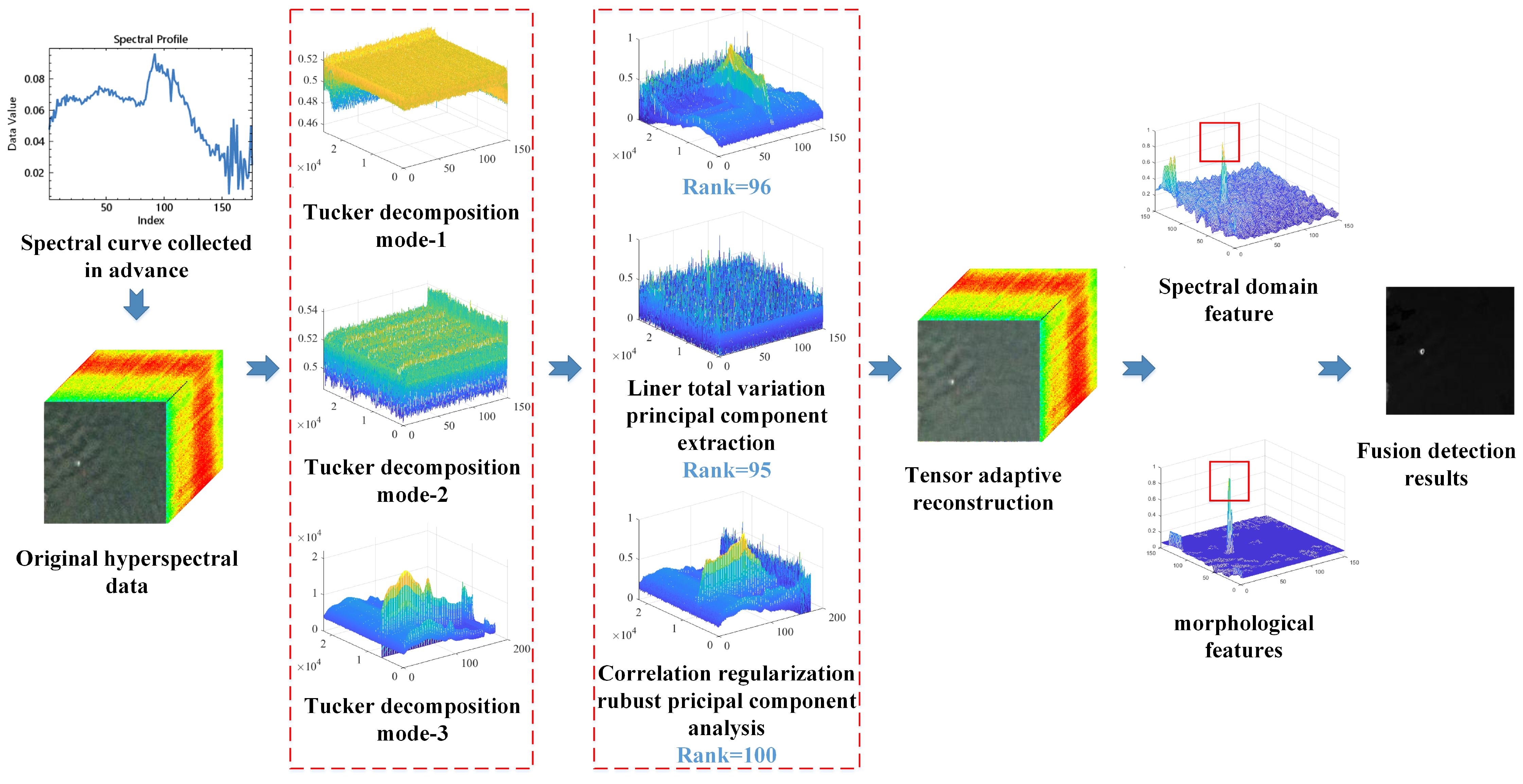
Figure 2. The target detection framework of the proposed TRSSF algorithm includes most similar target position acquisition, tensor decomposition and adaptive reconstruction, and spatial-spectral combined detection. The most similar target position acquisition uses an MF. Tensor decomposition and adaptive reconstruction use a linear total variation and correlation regular robust principal component analysis model. Spatial-spectral combined detection uses adaptive CEM and multiple morphological profile strategies.

2.1 Most similar target position acquisition

The matched filter is employed to locate similar target pixels in images (DiPietro et al., 2012). The likelihood ratio $\text{Λ}(\mathit{\text{h}})$ is determined by the Equation 1:

$\begin{array}{ll}\text{Λ}(h)=\frac{p(h|\text{Tp})}{p(h|\text{Ta})},& (1)\end{array}$

where Tp means target present and Ta means target absent. If Λ(h) exceeds the threshold, Tp is accepted, otherwise, Ta is accepted.

The probability density function follows a normal distribution model, which is expressed as Equation 2:

$\begin{array}{ll}\begin{array}{ll}{H}_0:h\sim N(u_{\text{b}},{\text{Σ}}_{\text{b}})\hfill & \text{Ta}\hfill \\ H_1:h\sim N(u_{\text{t}},{\text{Σ}}_{\text{t}})\hfill & \text{Tp},\hfill \end{array}& (2)\end{array}$

where ${\mathit{\text{u}}}_b$ and ${\mathit{\text{u}}}_t$ are the mean of the target and background, respectively. ${\Sigma }_{\text{b}}$ and ${\Sigma }_{\text{t}}$ represent the covariance matrix of the target and background, respectively. The matched filter based on background statistics is as Equation 3 (Akhter et al., 2014):

$\begin{array}{ll}{r}_{\text{MF}}(h)=\frac{{(t-u_{\text{t}})}^T{\Sigma }_{\text{b}}^{-1}(h-u_{\text{b}})}{{(t-{\mathit{u}}_{\text{t}})}^T{\Sigma }_{\text{b}}^{-1}(t-u_{\text{t}})},& (3)\end{array}$

where $t$ denotes the prior spectrum, $h$ denotes the pixel-tested spectrum, and ${\Sigma }_{\text{b}}^{-1}$ refers to the background matrix inversion operation.

Based on the similarity obtained, the target with the highest degree of similarity to the prior information is selected to obtain the target’s position within the image. The spectrum of the reconstruction data in this position is used as follow-up prior spectrum. The formula is as Equation 4:

$\begin{array}{ll}po=find(r_{\text{MF}}==max(r_{\text{MF}})),& (4)\end{array}$

where po is the position of the subsequent need.

2.2 Tensor decomposition and adaptive reconstruction of the hyperspectral data

In Figure 3, the hyperspectral image along with the expansion’s singular value distributions for modes 1, 2, and 3 are displayed. The rapid convergence of the curves shows that each mode’s decomposition possesses a low rank. The low rank characteristic can apply to hyperspectral tensor adaptive reconstruction.

Figure 3

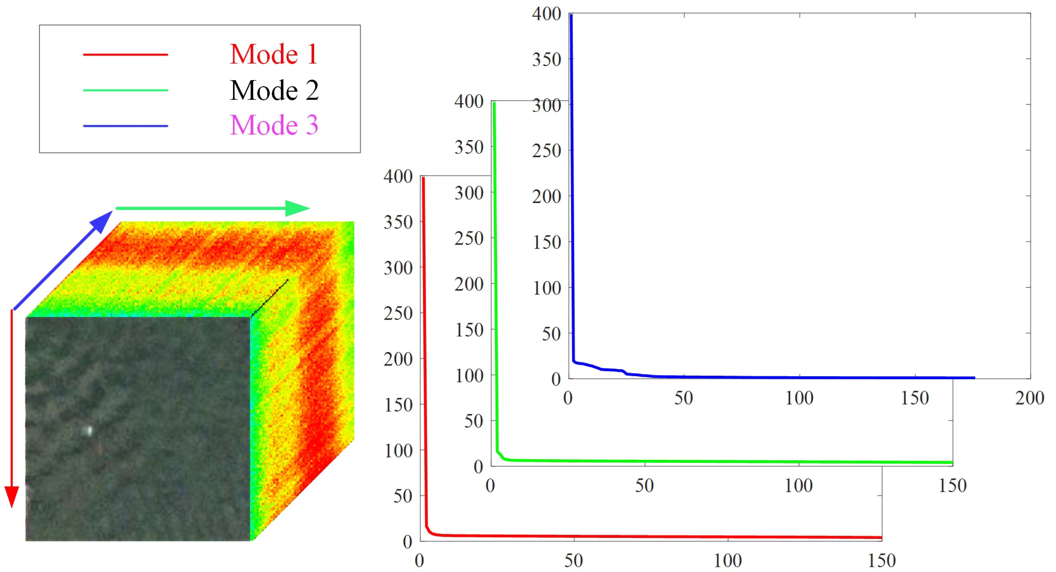
Figure 3. The singular value distribution of the hyperspectral image is unfolded across modes 1, 2, and 3.

2.2.1 Decomposition of the tensor using tucker decomposition

The hyperspectral image is represented as the tensor $\mathcal{D}\in {ℝ}^{T_1\times T_2\times T_3}$, where T₁, T₂ and T₃ represent the row, column, and band, respectively (Hou et al., 2021). Owing to the influence of several factors (topography, illumination, etc.), there are certain differences in the target spectral curve in the complex background. Tucker decomposition can effectively preserve the three-dimensional structural details of the data and eliminate other impurity signals, which is essential for the background complex hyperspectral images. They provide simple compression to maintain the principal components of the different factor matrices, thus increasing the distinction between target and background in complex background images. Therefore, Tucker decomposition and reconstruction of hyperspectral datasets is performed to obtain more stable feature-enhanced target and background separability. The Tucker decomposition formula is as Equation 5:

$\begin{array}{ll}\mathcal{D} \approx \mathcal{G}{\times }_{1}P{\times }_{2}Q{\times }_{3}W,& (5)\end{array}$

where $\mathcal{G}\in {ℝ}^{T_1\times T_2\times T_3}$ denotes the core tensor, signifying the degree of interaction among distinct components $P\in {ℝ}^{T_2{T}_3\times T_1}$, $Q\in {ℝ}^{T_1{T}_3\times T_2}$ and $W\in {ℝ}^{T_1{T}_2\times T_3}$ denote three factor matrices. They are the principal components for each mode. It is optimized as Equation 6:

$\begin{array}{ll}\begin{array}{l}\underset{\mathcal{G},P,Q,W}{\text{arg min}}{\Vert \mathcal{D}-\mathcal{G}{\times }_{1}P{\times }_{2}Q{\times }_{3}W\Vert }_2\hfill \\ \text{s}.\text{t}.\{\begin{array}{l}\mathcal{G}\in {ℝ}^{T_1\times T_2\times T_3}\hfill \\ P\in {ℝ}^{T_2{T}_3\times T_1},Q\in {ℝ}^{T_1{T}_3\times T_2},W\in {ℝ}^{T_1{T}_2\times T_3}\hfill \\ P^{T}P={\mathit{\text{I}}}_1,Q^{T}Q={\mathit{I}}_2,W^{T}W={\mathit{\text{I}}}_3\hfill \end{array}\hfill \end{array}.& (6)\end{array}$

The equation above is typically solved using the alternating least squares method. When the two matrices remain constant, an additional factor matrix is acquired through characteristic value decomposition.

2.2.2 Linear total variation smoothing robust principal component analysis

Tucker decomposition provides a simple compression method and can retain the most important information (Li et al., 2018; Xu et al., 2019). Because each factor matrix has different eigenvalues, their capacity to capture significant information also varies. Determining the appropriate numbers for ${\mathit{\text{r}}}_i$ (i is 1, 2, 3) is crucial for distinct factor matrices $(P,Q,W)$.

To mitigate the influence of noise on principal component extraction, this article applies total variation processing to the spatial dimension of the hyperspectral data. Total variation is defined as the difference between adjacent pixels (He et al., 2015). The total variation formula is as Equation 7:

$\begin{array}{ll}V(i,j)=\{\begin{array}{l}V(i+1,j)-V(i,j)\text{\hspace{1em} \hspace{0.17em} if \hspace{0.17em} \hspace{1em}}i<m\hfill \\ V(1,j)-V(i,j)\text{\hspace{1em} \hspace{0.17em} if \hspace{0.17em} \hspace{1em}}i=m\hfill \end{array},& (7)\end{array}$

where m denotes the number of columns of $V$. The total variation formula of $P$ is as Equation 8:

$\begin{array}{ll}{P}_{\text{TV}}(i,j)=\{\begin{array}{l}P(i,j+1)-P(i,j),\text{ if }j<T_1\hfill \\ P(i,1)-P(i,j),\text{ if }j=T_1\hfill \end{array}.& (8)\end{array}$

The total variation formula of $Q$ is as Equation 9:

$\begin{array}{ll}{Q}_{\text{TV}}(i,j)=\{\begin{array}{l}Q(i,j+1)-Q(i,j),\text{\hspace{1em} \hspace{0.17em} if \hspace{0.17em} \hspace{1em}}j<T_2\hfill \\ Q(i,1)-Q(i,j),\text{\hspace{1em} \hspace{0.17em} if \hspace{0.17em} \hspace{1em}}j=T_2\hfill \end{array}.& (9)\end{array}$

In the hyperspectral image, the background components are highly correlated; therefore, it is considered low rank. After the spatial dimension is smoothed, the robust principal component analysis method (RPCA) is used to acquire the data’s rank. Its formula is as Equation 10:

$\begin{array}{ll}\begin{array}{l}\underset{T,M}{\min }\text{ rank}(M)+\lambda \Vert T{\Vert }_0\hfill \\ \text{s}.\text{t}.M+T=X,\hfill \end{array}& (10)\end{array}$

where $M\in {ℝ}^{T_1{T}_3\times T_2}$ represents the low rank matrix, $T\in {ℝ}^{T_1{T}_3\times T_2}$ represents the sparse matrix, $X\in {ℝ}^{T_1{T}_3\times T_2}$ represents the unfolding of the original data, and $\lambda$ denotes a positive parameter regulating sparsity. Relaxing Equation 10 yields a manageable optimization problem. The $L_1$ norm is used to replace the $L_0$ norm, while the nuclear norm is used to replace the rank. It can transform into solving the Equation 11:

$\begin{array}{ll}\begin{array}{l}\underset{T,M}{\min }\Vert M{\Vert }_{*}+\lambda \Vert T{\Vert }_1\hfill \\ \text{s}.\text{t}.M+T=X.\hfill \end{array}& (11)\end{array}$

The original RPCA work in Candès et al. (2011) introduced an iterative thresholding method of low complexity with poor convergence. The alternating direction method of multipliers strategy is extensively used in optimization problems, which has good convergence (Kang et al., 2015). Therefore, it is adopted to solve this issue. It is as Equation 12:

$\begin{array}{ll}\begin{array}{l}L(M,T,Y,\mu )=\Vert M{\Vert }_{*}+\lambda \Vert T{\Vert }_1+\langle Y,X-M-T\rangle \hfill \\ +\frac{\mu }{2}\Vert X-M-T{\Vert }_F^2\hfill \\ =\Vert M{\Vert }_{*}+\lambda \Vert T{\Vert }_1+\frac{\mu }{2}{\Vert X-M-T+\frac{Y}{\mu }\Vert }_F^2-\frac{1}{2\mu }\Vert Y{\Vert }_F^2,\hfill \end{array}& (12)\end{array}$

where Y denotes the Lagrangian multiplier matrix, μ denotes the positive penalty scalar, $\langle ,\rangle$ is the inner product, and ${\Vert \Vert }_F^2$ signifies the Frobenius norm. The adopted algorithm involves updating the variables M, T and Y by minimizing function L while keeping the other variables fixed.

(1) Updating $M_k$: when other parameters are fixed, $M_k$ is obtained by solving the Equations 13 and 14:

$\begin{array}{ll}{M}_{k+1}\leftarrow \underset{A}{\text{arg min }}\frac{1}{\mu }\Vert M{\Vert }_k+\frac{1}{2}\Vert X-M-T_k+{\frac{Y_1}{\mu }\Vert }_F^2,& (13)\end{array}$

$\begin{array}{ll}{M}_{k+1}={\text{Θ}}_{{\mu }_k^{-1}}(X-T_k+{\mu }_k^{-1}{Y}_k),& (14)\end{array}$

where Θ denotes the singular value threshold operator and k is the number of iterations.

(2) Updating ${\mathit{\text{T}}}_k$: when other parameters are fixed, ${\mathit{\text{T}}}_k$ is obtained by solving the Equations 15 and 16:

$\begin{array}{ll}\begin{array}{c}{T}_{k+1}\leftarrow \underset{E}{\text{arg min }}\frac{\lambda }{2\mu }\Vert T{\Vert }_1\\ +\frac{1}{2}\Vert X-M_{k+1}+{\frac{Y_1}{\mu }\Vert }_F^2\end{array},& (15)\end{array}$

$\begin{array}{ll}{T}_{k+1}=S_{\lambda {\mu }_k^{-1}}[X-M_{k+1}+{\mu }_k^{-1}{Y}_k],& (16)\end{array}$

where $S_{\lambda {\mu }_k^{-1}}$ is the shrinkage operator (He et al., 2011); it is expressed as Equation 17:

$\begin{array}{ll}{S}_{Ɛ}(x)=\text{sgn}(x)\text{ max}(\left|x\right|-Ɛ,0).& (17)\end{array}$

(3) Updating $Y_k$ and ${\mu }_k$: they are obtained by solving the Equations 18 and 19:

$\begin{array}{ll}{Y}_{k+1}=Y_k+{\mu }_k(X-M_{k+1}-T_{k+1}),& (18)\end{array}$

$\begin{array}{ll}{\mu }_{k+1}=\rho {\mu }_k.& (19)\end{array}$

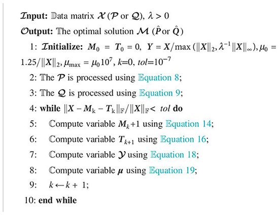
By solving the above formula, the low rank matrix $M$ ($\widehat{P}$ or $\widehat{Q}$) is acquired. The appropriate rank of the matrix is adaptively obtained. The outlined workflow is encapsulated in Algorithm 1.

2.2.3 Correlation regular robust principal component analysis

In the direction of expansion along a spectral dimension, to obtain the target that is closer to the prior spectrum, the minimum regular constraint for the tested and prior spectrums’ difference is added to the RPCA. It is as Equation 20:

$\begin{array}{ll}\begin{array}{c}\underset{M,T}{\min }\Vert M{\Vert }_{*}+\lambda \Vert T{\Vert }_1+\beta \Vert H\odot T-\mathit{\text{D}}\Vert \\ \text{s}.\text{t}.M+T=X,\end{array}& (20)\end{array}$

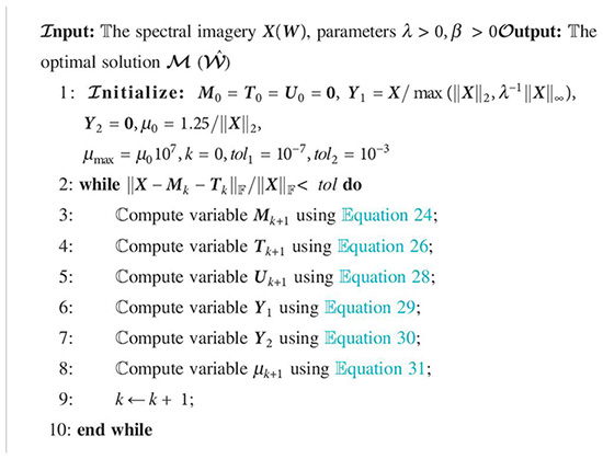
Algorithm 1. The linear total variation smoothing framework.

where ⊙ is the Hardman product, H is the spectral all-one matrix of the prior position, and D is the prior spectral matrix. The formula is displaced as Equation 21:

$\begin{array}{ll}\begin{array}{c}\underset{M,T}{\min }\Vert M{\Vert }_k+\lambda \Vert T{\Vert }_1+\beta \Vert H\odot U-D{\Vert }_F^2\\ \text{s}.\text{t}.M+T=X,U=T.\end{array}& (21)\end{array}$

The augmented Lagrangian function is as Equation 22:

$\begin{array}{ll}\begin{array}{l}\mathit{\text{L}}(M,T,U,Y1,Y2)\hfill \\ =\Vert M{\Vert }_{*}+\lambda \Vert T{\Vert }_1+\beta \Vert H\odot \mathit{\text{U}}-\mathit{\text{D}}{\Vert }_F^2\hfill \\ +\langle Y_1,X-M-T\rangle +\langle Y_2,\mathit{\text{T}}-\mathit{\text{U}}\rangle \hfill \\ +\frac{\mu }{2}({\Vert X-M-T\Vert }_F^2+{\Vert T-\mathit{\text{U}}\Vert }_F^2)\hfill \\ =\Vert M{\Vert }_{*}+\lambda \Vert \mathit{\text{T}}{\Vert }_1+\beta \Vert H\odot \mathit{\text{U}}-\mathit{\text{D}}{\Vert }_F^2\hfill \\ -\frac{\mu }{2\mu }({\Vert Y_1\Vert }_F^2+{\Vert Y_2\Vert }_F^2)\hfill \\ +\frac{\mu }{2}({\Vert X-M-T+\frac{Y_1}{\mu }\Vert }_F^2+{\Vert T-\mathit{\text{U}}+\frac{Y_2}{\mu }\Vert }_F^2)\hfill \end{array}& (22)\end{array}$

where $Y_1$ and $Y_2$ are the Lagrangian multiplier matrices, $\beta$ and µ are the positive penalty scalar, ${\Vert \Vert }_F^2$ symbolizes the Frobenius norm, and $\langle ,\rangle$ denotes the inner product. The solution involves updating the variables M, T, U, $Y_1$ and $Y_2$ by minimizing L while keeping other variables fixed.

(1) Updating $M_k$: when other variables are fixed, $M_k$ is obtained by computing the Equations 23 and 24:

$\begin{array}{ll}{M}_{k+1}\leftarrow \text{arg min }\frac{1}{\mu }\Vert M{\Vert }_{*}+\frac{1}{2}\Vert X-M-T_K+{\frac{Y_1}{\mu }\Vert }_F^2,& (23)\end{array}$

$\begin{array}{ll}{M}_{k+1}=\text{Θ}(X-T_k+{\mu }_k^{-1}{Y}_k).& (24)\end{array}$

(2) Updating $T_k$: when other parameters are fixed, $T_k$ is obtained by solving the Equations 25 and 26:

$\begin{array}{ll}\begin{array}{l}{T}_{K+1}\leftarrow \text{arg min }\frac{\lambda }{2\mu }\Vert T{\Vert }_1+\hfill \\ \frac{1}{2}{\Vert T-\frac{1}{2}\left({\mathit{\text{U}}}_{\mathit{\text{K}}}-\frac{Y_2}{\mu }+X-M_{\mathit{\text{K}}+1}+\frac{Y_1}{\mu }\right)\Vert }_F^2,\hfill \end{array}& (25)\end{array}$

$\begin{array}{ll}{T}_{k+1}={\text{S}}_{\lambda /(2\mu )}[\frac{1}{2}\left({\mathit{\text{U}}}_{\mathit{\text{K}}}-\frac{Y_2}{\mu }+X-M_{K+1}+\frac{Y_1}{\mu }\right].& (26)\end{array}$

(3) Updating $U_k$: when other parameters are fixed, $U_k$ is obtained by solving the Equations 27 and 28:

$\begin{array}{ll}{\mathit{\text{U}}}_{\mathit{\text{k}}+\mathbf{1}}\leftarrow \underset{U}{\text{arg min }}\frac{\beta }{\mu }\Vert H\odot \mathit{\text{U}}-\mathit{\text{D}}{\Vert }_F^2+\frac{1}{2}{\Vert \mathit{\text{U}}-T_{k+1}-\frac{Y_2}{\mu }\Vert }_F^2,& (27)\end{array}$

$\begin{array}{ll}{\mathit{\text{U}}}_{k+1}=\left(\frac{1}{\text{H}+\text{O}}\right)\odot \left(\mathit{\text{D}}+T_{k+1}+\frac{Y_2}{\mu }\right),& (28)\end{array}$

where $\text{O}$ is a matrix of all ones.

(4) Updating $Y_1$, $Y_2$ and ${\mu }_k$: $Y_k$ and ${\mu }_k$ are obtained by solving the Equations 29–31:

$\begin{array}{ll}{Y}_1\leftarrow Y_1+{\mu }_k(X-M_{k+1}-T_{k+1}),& (29)\end{array}$

$\begin{array}{ll}{Y}_2\leftarrow Y_2+{\mu }_k(T_{k+1}-U_{k+1}),& (30)\end{array}$

$\begin{array}{ll}{\mu }_{k+1}=\rho {\mu }_k.& (31)\end{array}$

By solving the above formula, the low-rank variable $U(\widehat{W})$ is obtained, and the appropriate rank of the matrix is adaptively obtained. The outlined method is summarized in Algorithm 2.

Algorithm 2. The framework of correlation regular robust principal component analysis.

In the adaptive acquisition of the rank (r1, r2 and r3) of the three factor matrices, tensor restoration is used to recover the hyperspectral three-dimensional images in which it is easy to detect the target. The reconstructed data have the same spectral dimension and are calculated as Equation 32:

$\begin{array}{ll}\tilde{\mathcal{D}}\approx {\mathcal{G}}_r{\times }_1{P}_{r1}{\times }_2{Q}_{r2}{\times }_3{W}_{r3},& (32)\end{array}$

where $P_{r1}=P(:,1:r1),Q_{r2}=Q(:,1:r2),W_{r3}=W(:,1:r3)$ and ${\mathcal{G}}_r$ = $\mathcal{G}$ (1: r1, 1: r2, 1: r3).

The $r_i(i\in 1,2,3)$ signifies the count of principal components in distinct factor matrices.

The intrinsic features of the hyperspectral image can be effectively retained by tensors. In Figure 4, spectral curves of a randomly chosen target-target, as well as target-background pixels, are presented from the pollution dataset before and after tensor reconstruction. The legend O denotes the original data spectral profile and T denotes the reconstructed data spectral profile. In the 60 to 80 band of Figure 4A, the separation between the black lines is less than the separation between the red lines. In the 60 to 80 band of Figure 4B, the separation between the black lines is greater than the separation between the red lines. This confirms that after tensor processing, the distinction between the background and target spectra is increased.

Figure 4

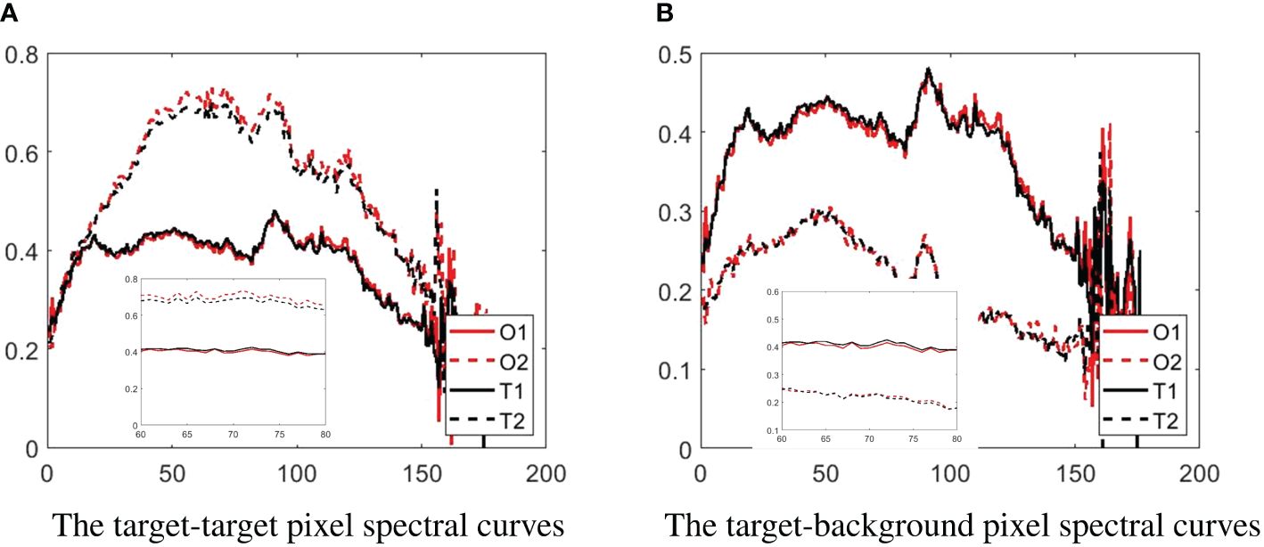
Figure 4. The spectral curves of target-target and target-background pixels are randomly chosen from the pollution dataset before and after Tucker decomposition and reconstruction. (A) The target-target pixel spectral curves. (B) The target-background pixel spectral curves.

2.3 Spatial-spectral combined detection

Existing hyperspectral target detection algorithms use less spatial information. To make up for these deficiencies and improve the performance of target detection, this study adopts a spatial-spectral combined detection method for reconstruction data.

In the spectral domain, an adaptive CEM detection method is proposed. Its design needs to satisfy the Equation 33:

$\begin{array}{ll}\{\begin{array}{l}\underset{q}{\text{min}}{\mathit{q}}^T\mathrm{Rq}\hfill \\ q^{T}d=1\hfill \end{array},& (33)\end{array}$

where $\mathit{q}$ is the filter, $\mathit{d}$ denotes the prior position spectrum, and $R$ denotes the correlation matrix. The optimal solution is as Equation 34:

$\begin{array}{ll}{q}^{*}=\frac{R^{-1}d}{d^T{R}^{-1}d}& (34)\end{array}$

After derivation, the spectral domain result ${\mathit{r}}_{\text{ac}i}$ is as Equation 35:

$\begin{array}{ll}{r}_{\text{ac}i}=e{q}^{*T}{x}_i=e\frac{d^T{R}^{-1}{x}_i}{d^T{R}^{-1}d},& (35)\end{array}$

where ${\mathit{x}}_i$ represents the reconstructed data’s spectrum and e represents the mean of $L_2$ norm of the difference value between the pixels tested and its four neighborhoods.

In the spatial domain, similarity multiple morphological profile feature extraction is proposed. The similarity value is obtained by fusing the Pearson correlation coefficient with the prior spectrum’s Euclidean distance from the reconstructed data using the Equation 36:

$\begin{array}{ll}{r}_{\text{s}i}={\Vert x_i-d\Vert }_2+\frac{cov\left(x_i,d\right)}{{\delta }_{{\mathit{x}}_i}{\delta }_d},& (36)\end{array}$

where ${\Vert \Vert }_2$ is the L2 norm, cov denotes the covariance, δ denotes the standard deviation, ${\delta }_{\mathit{x}i}$ denotes the standard deviation of ${\mathit{x}}_i$, and ${\delta }_{\mathit{d}}$ denotes the standard deviation of d. Multiple morphological profiles obtain a multilevel representation of an image by constructing maximum and minimum trees and then using a series of attribute filtering operations, which can extract spatial, structural, and textural features in the image (Hou et al., 2021). The method has been applied in hyperspectral image classification (Aptoula et al., 2016; Bao et al., 2016). To maximize the use of spatial features for increased detection performance, the morphological feature extraction method is used to process the similarity results of the previous step. The multiple morphological profile formula adopted is as Equations 37–41:

$\begin{array}{ll}\text{Area }(C)=\{\#l|l\in C\},& (37)\end{array}$

$\begin{array}{ll}\text{Height }(C)=\underset{l\in C}{\max }f(l)-\underset{l\in C}{\min }f(l),& (38)\end{array}$

$\begin{array}{ll}\text{Volume }(C)=\sum _{l\in C}\left(\underset{l\in C}{\max }v(l)-v(l)\right),& (39)\end{array}$

$\begin{array}{ll}\text{Diag }(C)=\sqrt{{(x_{l,\max }-x_{l,\min })}^2+{(y_{l,\max }-y_{l,\min })}^2},& (40)\end{array}$

$\begin{array}{ll}\text{Std }(C)=\sqrt{\frac{1}{\text{Area} (C)}\sum _{\forall l\in C}(f(l)-K_{\text{gray}-\text{level }}(\lambda ))},& (41)\end{array}$

where C is the connected region, # is the number of pixels in the connection area, l represents the pixel within the connected region, $f(l)$ denotes the function to obtain the value of the l pixel, and $v=\pm f,x_{l,\min },x_{l,\max }$ and $y_{l,\min }$, $y_{l,\max }$ denote these extremes for the horizontal and vertical coordinates of the region that is connected, respectively. $K_{\text{gray}-\text{level}}$ denotes the average intensity of pixels within the connected region.

The multiple morphological feature fusion is as Equation 42:

$\begin{array}{ll}{R}_{\text{MMF}}=R_{kk,\min }-R_{ll,\max },& (42)\end{array}$

where $R_{\text{MMF}}$ is the result of the fusion of multiple morphological features, $R_{kk,\min }$ and $R_{ll,\max }$ denote smaller pruning for attribute kk and larger pruning for attribute ll, respectively. kk and ll belong to the above five morphologies.

Figure 5 demonstrates pruning and reconstruction using multiple morphological attributes (area and height) of the maximal tree. Target features can be preserved by using the fusion of area 5 with height 1 pruning value 5 results. Therefore, targets can be extracted using this multiple morphological feature fusion.

Figure 5

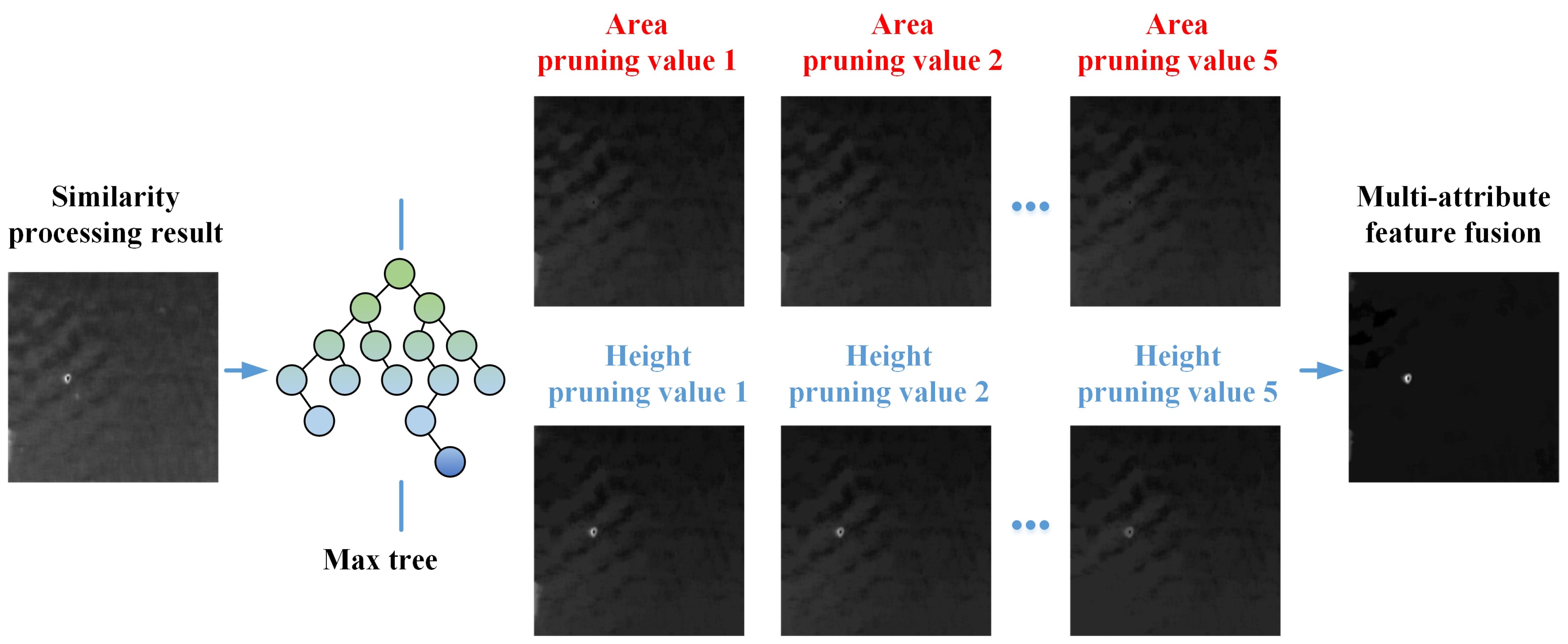
Figure 5. Schematic of pruning and fusion using multiple morphological attributes.

After obtaining the spectral and spatial domain results, the spatial-spectrum fusion is realized by the Equation 43:

$\begin{array}{ll}R=b{R}_{\text{ac}}+(1-b)R_{\text{MMF}},& (43)\end{array}$

where b is the weighting factor, $R_{\text{ac}}$ is the result of spectral detection, and $R_{\text{MMF}}$ is the result of spatial detection. The framework of TRSSF is summarized in Algorithm 3.

Algorithm 3. The framework of the proposed TRSSF.

Figure 6 illustrates the receiver operating characteristic curve (ROC) of the tensor adaptive restruct spectral feature (TS), tensor adaptive restruct morphological feature (TM), and proposed TRSSF. Across the four datasets, the ROCs of the proposed methods TS, TM, and TRSSF all reside near the upper left corner, indicating a strong performance for all the proposed algorithms. Out of the four images, the TRSSF algorithm’s ROC curves are closest to the upper left, indicating a superior performance for the tensor adaptive restructured and spatial-temporal fusion algorithm. From Table 1, it can also be observed that the spectral characteristics and morphological features have high area under the curve (AUC) values, and the spatial spectral fusion method AUC values increase very significantly.

Figure 6

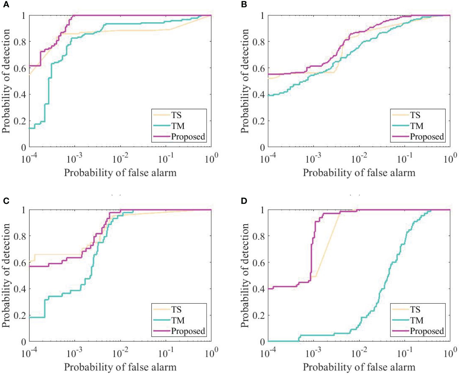
Figure 6. The ROC curve for different datasets. (A) Ship. (B) Wake. (C) Pollution. (D) Floating object.

Table 1

Table 1. AUC values of the tensor adaptive restruct spectral feature (TS), tensor adaptive restruct morphological feature (TM), and TRSSF on four datasets.

In summary, a tensor adaptive reconstruction cascade spatial-spectral fusion algorithm is proposed for hyperspectral target detection. First, the matched filter method is adopted to acquire the position of the pixel that best matches the prior spectrum. Second, tensor Tucker decomposition and reconstruction by linear total variation smoothing robust principal component analysis and correlation regular robust principal component analysis are used to improve the differentiation between the target and background. Finally, the spatial-spectral fusion method is proposed to acquire the required target pixels.

3 Experiments and analysis

3.1 Hyperspectral datasets

The first data were collected by airborne HSI system SPECTIR sensors. The spatial resolution and spectral resolution of the sensor were 1 m and 5 nm, respectively. The target is the ship and the background is the nearshore water (Giannandrea et al., 2013). The target spectra were obtained from the images. The detailed description of the datasets can be found in row 1 of Table 2. In addition, the false-color image (PI) and ground truth image (GT) of these datasets are displayed in rows 1 and 2 of Figures 7A, B.

Table 2

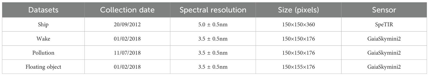
Table 2. Detailed description of the hyperspectral datasets.

Figure 7

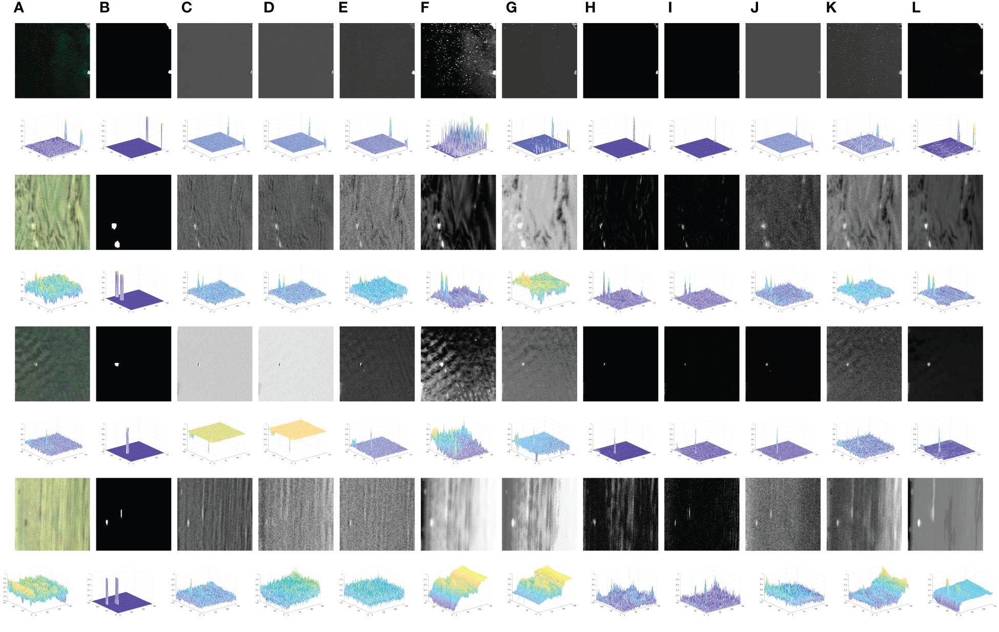
Figure 7. The pseudo-color image, ground truth map, and detection results of 10 methods in the four datasets. (A) Pseudo-color image. (B) Ground truth map. (C) CEM. (D) MF. (E) MOBS. (F) IEEPST. (G) LCNN. (H) DSC. (I) TRPCAF. (J) PTA. (K) TTDL. (L) Proposed.

The second to fourth hyperspectral datasets were collected by the Dualix spectral imaging instrument GaiaSkymini2. Its spectral range spans from 400 nm to 1,000 nm, the spatial resolution is 0.14 m, and the spectral resolution is 3.5 nm. Targets include wake, oil, and floating objects. The background includes the sea at different times or in different situations. Prior target spectra are collected in advance from these targets in real scenes. A detailed description of the dataset is presented in rows 2 to 4 of Table 2. The PI and GT for the dataset are presented in Figures 7A, B within rows 3 to 8.

3.2 Evaluation indicators and analysis

To conduct qualitative and quantitative analyses, we used the detection result map, compared target-background separability, and introduced metrics such as detection probability (PD), false alarm probability (PF), and ROC.

Detection result maps are presented in grayscale, in which brighter shades indicate a proximity to the target. These maps provide a direct depiction of the target’s location. The algorithm’s performance is assessed based on the count of correct and erroneous pixels.

In the box plot, the central line denotes the median value and the box’s upper and lower edges denote 75% and 25% of the maximum values, respectively. The “whiskers” represent the extreme values of the detection results. The red box delineates the target value in detection results, whereas the green box delineates the background value in detection outcomes. The separation ability of the target background for the detection results is indicated by the distance between the green and red boxes (Hou et al., 2021). A larger distance signifies better algorithm performance.

Points on the ROC curve indicate the PDs at various PFs. The proximity of the ROC curve to top-left corner of the coordinate axis indicates superior detection results for the algorithm. PD quantifies the proportion of correctly detected pixels relative to the overall count of target pixels. PF denotes the proportion of background pixels erroneously classified as targets relative to the background pixel count (Li et al., 2021, 2022b). At a given PF value, higher PD values signify better algorithm performance (Zhao et al., 2022; Liu et al., 2023; Ge et al., 2024). The PD and PF can be calculated by Equations 44, 45:

$\begin{array}{ll}PD=\frac{N_d}{N_t},& (44)\end{array}$

$\begin{array}{ll}PF=\frac{N_f}{N_b},& (45)\end{array}$

where $N_d$, $N_t$, $N_f$, and $N_b$ represent the number of correctly detected pixels, actual target pixels, pixels erroneously detected, and background pixels in the image, respectively. After getting an array corresponding to the PD and PF, the AUC is displayed as Equation 46:

$\begin{array}{ll}AUC=\frac{1}{2}\times \sum _i^{nn}(P{F}_i-P{F}_{i-1})\times (P{D}_i+P{D}_{i-1}),& (46)\end{array}$

where nn denotes the number of thresholds, $i\in 1,2,\dots ,nn$.

3.3 Detection performance

The parameters in this experiment encompass λ and β. In the spatial dimensionality unfolding of data, the value of λ is $1/\sqrt{T_2{T}_3\times T_1}$ or $1/\sqrt{T_1{T}_3\times T_2}$. In the spectral dimensionality unfolding of data, the value of λ is $1/\sqrt{T_1{T}_2\times T_3}$, and the value of β range is [10¹, 10², 10³, 10⁴, 10⁵]. It is found through experiments that these two parameters have little effect on the experimental results, and the value of β used in this experiment was 10¹. T₁, T₂ and T₃ represent the rows, columns, and bands for the hyperspectral image, respectively. The comparison algorithms used in this study were as follows: CEM (Farrand and Harsanyi, 1997), MF (Manolakis et al., 2009), MOBS (Sun et al., 2024b), IEEPST (Sun et al., 2024c), LCNN (Dong et al., 2023), DSC (Zhang et al., 2020), TRPCAF (Chen and Wang, 2019), and PTA (Li et al., 2020), TTDL (Zhao et al., 2020a).

Figure 7 visually depicts the detection results using different algorithms across the four datasets. The proposed TRSSF algorithm demonstrates superior detection capability, identifying more target pixels across these datasets with minimal false alarms. In contrast, other comparison methods exhibit poor detection results. In rows 1 and 2 (Figure 7I), TRPCAF can barely detect the target. In rows 1 and 2 (Figures 7C–E, H, J), CEM, MF, MOBS, DSC, and PTA identify some correct pixels. In rows 1 and 2 (Figures 7F, G, K), IEEPST, LCNN, and TTDL can detect more target pixels but some error pixels are also detected. In rows 3 and 4 (h) and (i) of Figure 7, DSC and TRPCAF detect very few correct pixels. In rows 3 and 4 (Figures 7C–G, J, K), CEM, MF, MOBS, IEEPST, LCNN, PTA, and TTDL identify more correct pixels, albeit with numerous erroneous background pixels also detected. In rows 5 and 6 (Figures 7C–G, J, K), CEM, MF, DSC, TRPCAF, and PTA detect fewer correct pixels. In rows 5 and 6 (Figures 7E–G, K), MOBS, IEEPST, LCNN, and TTDL can check more target pixels but also identify numerous false positives. In rows 7 and 8 (Figure 7I), TRPCAF detect fewer correct pixels. In rows 7 and 8 (Figures 7C–H, J, K), CEM, MF, MOBS, IEEPST, LCNN, DSC, PTA, and TTDL can identify more target pixels but also identify numerous false positives. Therefore, the proposed TRSSF has good detection performance.

Figure 8 shows a box plot diagram comparing the detection results across the four datasets using different methods. In Figure 8B, the green and red boxes’ distance of LCNN and IEEPST are greater than the proposed TRSSF algorithm. In Figure 8C, the green and red boxes’ distance of IEEPST is greater than the proposed TRSSF algorithm. However, the red and green boxes’ distance in TRSSF are greater than those with the other algorithms. In Figures 8A, D, the green and red boxes separation of the TRSSF algorithm is greater those of the other algorithms, which can easily obtain the desired target from the images. Some of the remaining algorithms even have a partial overlap in the green and red boxes of the detection results. Therefore, the TRSSF’s separation is better.

Figure 8

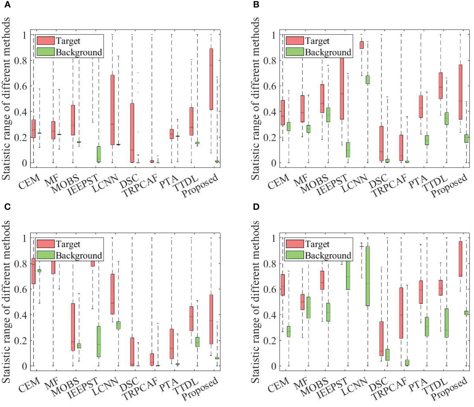
Figure 8. Statistical separability analysis of 10 methods in the four datasets. (A) Ship. (B) Wake. (C) Pollution. (D) Floating object.

Figure 9 displays the ROC for various algorithms used to detect the results across the four datasets. In Figure 9A, when the PF was approximately 0.1, the corresponding PD for TRSSF was approximately 1.0000. The PDs for all comparative methods (CEM, MF, MOBS, IEEPST, LCNN, DSC, TRPCAF, PTA, and TTDL) were 0.6167, 0.6000, 0.8667, 1.0000, 0.7500, 0.8417, 0.8250, 0.6000, and 0.8167, respectively. In Figures 9B–D, when the PFs were all 0.1, the PDs for TRSSF were 0.9902, 1.0000, and 1.0000. The biggest PDs among other baseline methods were 0.9805, 1.0000, and 0.9231. The proposed method’s ROC curves were consistently closest to the upper left of the coordinate axis. The efficacy of the TRSSF algorithm was confirmed through an evaluation using the aforementioned four hyperspectral datasets.

Figure 9

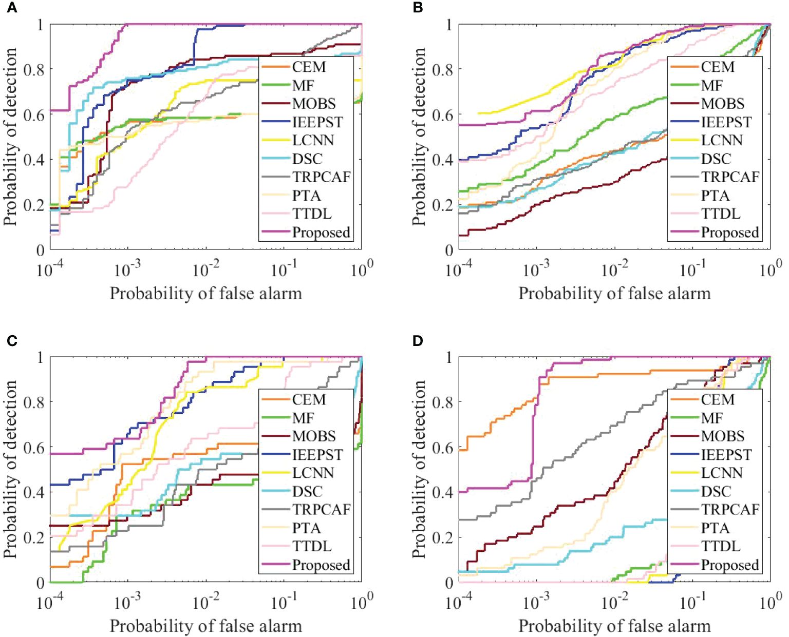
Figure 9. The ROC curve with different datasets. (A) Ship. (B) Wake. (C) Pollution. (D) Floating object.

Table 3 presents the AUC values for the aforementioned ten algorithms. On four different datasets, the TRSSF’s AUCs were 0.9998, 0.9934, 0.9986, and 0.9993, respectively. The maximum AUC values for all comparison algorithms across the four real scenarios were 0.9979, 0.9908, 0.9935, and 0.9376, respectively. The minimum AUC values for all comparison methods across the four real scenarios were 0.6338, 0.7539, 0.5518, and 0.6208, respectively. All of them were lower than the AUC value of the TRSSF. The TRSSF’s detection performance is optimal.

Table 3

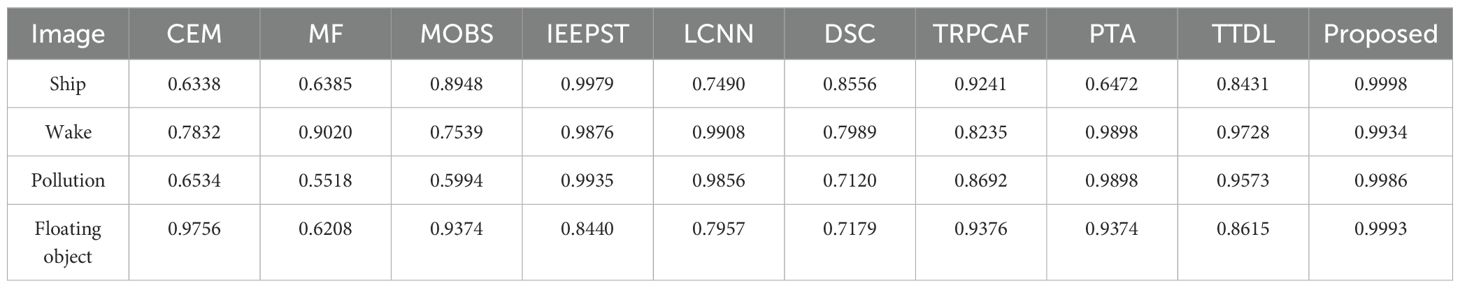
Table 3. AUC values of different methods on four datasets.

Table 4 presents the execution times of all the methods in different datasets. The times consumed by TRSSF were 41.5543 s, 20.3282 s, 41.0718 s, and 21.6437 s. The longest time consumed by the other methods on these datasets were 86.1928 s, 49.0279 s, 42.7094 s, and 51.9833 s, respectively. The time consumed by PTA was the longest. The time consumed by TRSSF was more than the traditional methods but less than the spatial-spectral fusion methods. The proposed TRSSF not only exhibits excellent detection performance for complex scenes but also does not take long to execute. All algorithm tests were conducted using MATLAB on a computer with an Intel Core i7-8700 h CPU and 8GB of RAM.

Table 4

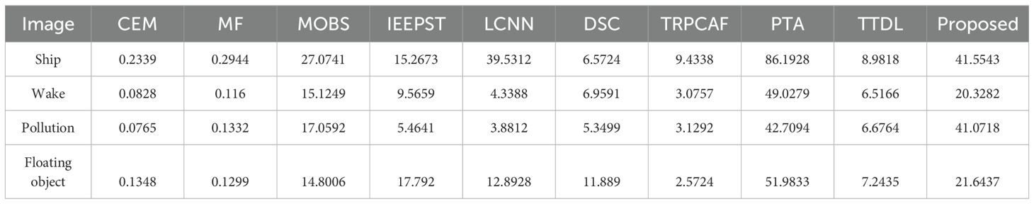
Table 4. Execution time of different methods on four datasets (unit: s).

4 Conclusion

This study proposed a tensor adaptive reconstruction cascade spatial-spectral fusion (TRSSF) method for marine pollutants detection. First, the position of the pixel with the highest degree of matching with the prior spectral curve was obtained. This position could obtain the prior spectrum of the subsequent matching detection. Second, the tensor decomposition and reconstruction method based on the total variation and prior constraint was processed to the initial hyperspectral image. In the spatial dimensionality unfolding of the data, the linear total variational RPCA method was employed to obtain its rank. In the spectral dimensionality unfolding of data, similarity regularization RPCA was employed to obtain its rank. The data were reconstructed according to an adaptively chosen rank. Finally, the spatial-spectral fusion method was used to select the optimal target from the reconstructed data. Experiments performed on publicly available and laboratory-collected hyperspectral datasets showcased the effective detection performance of the proposed approach.

In the future, as the application scenarios become more complex, the data will become increasingly larger. Too many bands in the hyperspectral data will result in the data containing a large amount of redundant information, which makes data processing and analysis more complicated and reduces the efficiency and detection rate of target detection. Therefore, hyperspectral target detection based on band selection will be the direction that will be studied in the next phase. At the same time, some existing hyperspectral moving targets have rich temporal information; therefore, the study of combining spatial and temporal information can further improve the target detection rate.

Data availability statement

The original contributions presented in the study are included in the article/supplementary material. Further inquiries can be directed to the corresponding author.

Author contributions

XZ: Writing – review & editing, Writing – original draft, Methodology, Funding acquisition, Data curation, Conceptualization. KG: Writing – review & editing. FH: Writing – review & editing. JC: Writing – review & editing. ZX: Writing – review & editing. LS: Writing – review & editing. ML: Writing – review & editing.

Funding

The author(s) declare financial support was received for the research, authorship, and/or publication of this article. This research was partly supported by the Postdoctoral Science Foundation of China under Grant 2023M740240 and partly supported by the Open Project of Fujian Key Laboratory of Spatial Information Perception and Intelligent Processing (Yango University, Grant No. FKLSIPIP1018).

Conflict of interest

The authors declare that the research was conducted in the absence of any commercial or financial relationships that could be construed as a potential conflict of interest.

Publisher’s note

All claims expressed in this article are solely those of the authors and do not necessarily represent those of their affiliated organizations, or those of the publisher, the editors and the reviewers. Any product that may be evaluated in this article, or claim that may be made by its manufacturer, is not guaranteed or endorsed by the publisher.

References

Akhter M. A., Heylen R., Scheunders P. (2014). A geometric matched filter for hyperspectral target detection and partial unmixing. IEEE Geosci. Remote. Sens. Lett. 12, 661–665. doi: 10.1109/LGRS.2014.2355915

Crossref Full Text | Google Scholar

Aptoula E., Mura M. D., Lefèvre S. (2016). Vector attribute profiles for hyperspectral image classification. IEEE Trans. Geosci. Remote Sens. 54, 3208–3220. doi: 10.1109/TGRS.2015.2513424

Crossref Full Text | Google Scholar

Bao R., Xia J., Mura M. D., Du P., Chanussot J., Ren J. (2016). Combining morphological attribute profiles via an ensemble method for hyperspectral image classification. IEEE Geosci. Remote. Sens. Lett. 13, 359–363. doi: 10.1109/LGRS.2015.2513002

Crossref Full Text | Google Scholar

Cai J., Candès E., Shen Z. (2010). A singular value thresholding algorithm for matrix completion. SIAM J. Optim. 20, 1956–1982. doi: 10.1137/080738970

Crossref Full Text | Google Scholar

Candès E. J., Li X., Ma Y., Wright J. (2011). Robust principal component analysis. J. ACM 58, 1–37. doi: 10.1145/1970392.1970395

Crossref Full Text | Google Scholar

Chang C. (1999). “Spectral information divergence for hyperspectral image analysis,” in IEEE 1999 International Geoscience and Remote Sensing Symposium. IGARSS’99 (Cat. No. 99CH36293), Hamburg, Germany: IEEE Vol. 1. 509–511. doi: 10.1109/IGARSS.1999.773549

Crossref Full Text | Google Scholar

Chen X., Zhang M., Liu Y. (2024). Target detection with spectral graph contrast clustering assignment and spectral graph transformer in hyperspectral imagery. IEEE Trans. Geosci. Remote Sens. 62, 1–16. doi: 10.1109/TGRS.2024.3394616

Crossref Full Text | Google Scholar

Chen Y., Nasrabadi N., Tran T. (2011). Sparse representation for target detection in hyperspectral imagery. IEEE J. Sel. Top. Signal Process. 5, 629–640. doi: 10.1109/JSTSP.2011.2113170

Crossref Full Text | Google Scholar

Chen Z., Wang B. (2019). Hyperspectral target detection based on tensor sparse representation. IEEE Geosci. Remote. Sens. Lett. 16, 1605–1609. doi: 10.1109/LGRS.8859

Crossref Full Text | Google Scholar

Chen Z., Yang B., Wang B. (2018). A preprocessing method for hyperspectral target detection based on tensor principal component analysis. Remote Sens. 10, 1033–1053. doi: 10.3390/rs10071033

Crossref Full Text | Google Scholar

Coorey R. (2018). “The evolution of geospatial intelligence,” in Australian contributions to strategic and military geography, Midtown Manhattan, New York, USA: Springer 143–151.

Google Scholar

Dian R., Fang L., Li S. (2017). “Hyperspectral image super-resolution via non-local sparse tensor factorization,” in Proceedings of the IEEE conference on computer vision and pattern recognition, Honolulu, Hawaii: IEEE 5344–5353. doi: 10.1109/CVPR.2017.411

Crossref Full Text | Google Scholar

DiPietro R. S., Manolakis D. G., Lockwood R. B., Cooley T., Jacobson J. (2012). Hyperspectral matched filter with false-alarm mitigation. Opt. Eng. 51, 016202–016202. doi: 10.1117/1.OE.51.1.016202

Crossref Full Text | Google Scholar

Dong Y., Dai X., Zhang Y., Du B. (2023). A lightweight convolutional neural network based on joint correlation distance constraints and density peak clustering for hyperspectral target detection. IEEE Trans. Geosci. Remote Sens. 61, 1–14. doi: 10.1109/TGRS.2023.3292292

Crossref Full Text | Google Scholar

Dong W., Wu X., Qu J., Gamba P., Xiao S., Vizziello A., et al. (2024). Deep spatial–spectral joint-sparse prior encoding network for hyperspectral target detection. IEEE Trans. Cybern 54, 1–13. doi: 10.1109/TCYB.2024.3403729

Crossref Full Text | Google Scholar

Du B., Zhang L. (2010). Random-selection-based anomaly detector for hyperspectral imagery. IEEE Trans. Geosci. Remote Sens. 49, 1578–1589. doi: 10.1109/TGRS.2010.2081677

Crossref Full Text | Google Scholar

Farrand W. H., Harsanyi J. C. (1997). Mapping the distribution of mine tailings in the coeur d’alene river valley, idaho, through the use of a constrained energy minimization technique. Remote Sens. Environ. 59, 64–76. doi: 10.1016/S0034-4257(96)00080-6

Crossref Full Text | Google Scholar

Feng S., Tang S., Zhao C., Cui Y. (2021). A hyperspectral anomaly detection method based on low-rank and sparse decomposition with density peak guided collaborative representation. IEEE Trans. Geosci. Remote Sens. 60, 1–13. doi: 10.1109/TGRS.2021.3054736

Crossref Full Text | Google Scholar

Gao L., Wang D., Zhuang L., Sun X., Huang M., Plaza A. (2023). BS³LNet: A new blind-spot self-supervised learning network for hyperspectral anomaly detection. IEEE Trans. Geosci. Remote Sens. 61, 1–18. doi: 10.1109/TGRS.2023.3246565

Crossref Full Text | Google Scholar

Ge F., Xuan K., Lou P., Li J., Jiang L., Wang J., et al. (2024). Multi-object detection and behavior tracking of sea cucumbers with skin ulceration syndrome based on deep learning. Front. Mar. Sci. 11, 1365155. doi: 10.3389/fmars.2024.1365155

Crossref Full Text | Google Scholar

Giannandrea A., Raqueno N., Messinger D. W., Faulring J., Kerekes J. P., Van Aardt J., et al. (2013). “The share 2012 data campaign,” in Algorithms and technologies for multispectral, hyperspectral, and ultraspectral imagery XIX, vol. 8743. (Baltimore, Maryland, United States: SPIE), 94–108. doi: 10.1117/12.2015935

Crossref Full Text | Google Scholar

Guo X., Huang X., Zhang L., Zhang L. (2013). Hyperspectral image noise reduction based on rank-1 tensor decomposition. ISPRS J. Photogramm. Remote Sens. 83, 50–63. doi: 10.1016/j.isprsjprs.2013.06.001

Crossref Full Text | Google Scholar

Harsanyi J. C., Chang C.-I. (1994). Hyperspectral image classification and dimensionality reduction: An orthogonal subspace projection approach. IEEE Trans. Geosci. Remote Sens. 32, 779–785. doi: 10.1109/36.298007

Crossref Full Text | Google Scholar

He R., Hu B., Zheng W., Kong X. (2011). Robust principal component analysis based on maximum correntropy criterion. IEEE Trans. Image Process. 20, 1485–1494. doi: 10.1109/TIP.2010.2103949

PubMed Abstract | Crossref Full Text | Google Scholar

He W., Zhang H., Zhang L., Shen H. (2015). Total variation regularized low-rank matrix factorization for hyperspectral image restoration. IEEE Trans. Geosci. Remote Sens. 54, 178–188. doi: 10.1109/TGRS.2015.2452812

Crossref Full Text | Google Scholar

Hou Z., Li W., Li L., Tao R., Du Q. (2021). Hyperspectral change detection based on multiple morphological profiles. IEEE Trans. Geosci. Remote Sens. 60, 1–12. doi: 10.1109/TGRS.2021.3090802

Crossref Full Text | Google Scholar

Hou Z., Li W., Tao R., Ma P., Shi W. (2022). Collaborative representation with background purification and saliency weight for hyperspectral anomaly detection. Sci. China Inf. Sci. 65, 1–12. doi: 10.1007/s11432-020-2915-2

Crossref Full Text | Google Scholar

Kang Z., Peng C., Cheng Q. (2015). “Robust pca via nonconvex rank approximation,” in 2015 IEEE International Conference on Data Mining. 211–220 (Atlantic City, NJ, USA: IEEE). doi: 10.1109/ICDM.2015.15

Crossref Full Text | Google Scholar

Kolda T., Bader B. (2009). Tensor decompositions and applications. SIAM Rev. 51, 455–500. doi: 10.1137/07070111X

Crossref Full Text | Google Scholar

Kruse F. A., Lefkoff A., Boardman J., Heidebrecht K., Shapiro A., Barloon P., et al. (1993). The spectral image processing system (sips)—interactive visualization and analysis of imaging spectrometer data. Remote Sens. Environ. 44, 145–163. doi: 10.1016/0034-4257(93)90013-N

Crossref Full Text | Google Scholar

Li S., Dian R., Fang L., Bioucas-Dias J. (2018). Fusing hyperspectral and multispectral images via coupled sparse tensor factorization. IEEE Trans. Image Process. 27, 4118–4130. doi: 10.1109/TIP.2018.2836307

Crossref Full Text | Google Scholar

Li W., Du Q. (2016). A survey on representation-based classification and detection in hyperspectral remote sensing imagery. Pattern Recognit. Lett. 83, 115–123. doi: 10.1016/j.patrec.2015.09.010

Crossref Full Text | Google Scholar

Li L., Li W., Qu Y., Zhao C., Tao R., Du Q. (2020). Prior-based tensor approximation for anomaly detection in hyperspectral imagery. IEEE Trans. Neural Netw. Learn Syst. 33, 1037–1050. doi: 10.1109/TNNLS.2020.3038659

Crossref Full Text | Google Scholar

Li L., Ma H., Jia Z. (2021). Change detection from SAR images based on convolutional neural networks guided by saliency enhancement. Remote Sens. 13, 3697–3717. doi: 10.3390/rs13183697

Crossref Full Text | Google Scholar

Li L., Ma H., Jia Z. (2022b). Multiscale geometric analysis fusion-based unsupervised change detection in remote sensing images via flicm model. Entropy 24, 291. doi: 10.3390/e24020291

PubMed Abstract | Crossref Full Text | Google Scholar

Li J., Zheng K., Gao L., Ni L., Huang M., Chanussot J. (2024). Model-informed multistage unsupervised network for hyperspectral image super-resolution. IEEE Trans. Geosci. Remote Sens. 62, 1–17. doi: 10.1109/TGRS.2024.3391014

Crossref Full Text | Google Scholar

Li J., Zheng K., Li Z., Gao L., Jia X. (2023a). X-shaped interactive autoencoders with crossmodality mutual learning for unsupervised hyperspectral image super-resolution. IEEE Trans. Geosci. Remote Sens. 61, 1–17. doi: 10.1109/TGRS.2023.3300043

Crossref Full Text | Google Scholar

Li J., Zheng K., Liu W., Li Z., Yu H., Ni L. (2023b). Model-guided coarse-to-fine fusion network for unsupervised hyperspectral image super-resolution. IEEE Geosci. Remote Sens. Lett. 20, 1–5. doi: 10.1109/LGRS.2023.3309854

Crossref Full Text | Google Scholar

Li J., Zheng K., Yao J., Gao L., Hong D. (2022a). Deep unsupervised blind hyperspectral and multispectral data fusion. IEEE Geosci. Remote Sens. Lett. 19, 1–5. doi: 10.1109/LGRS.2022.3151779

Crossref Full Text | Google Scholar

Liu Y., Gao G., Gu Y. (2016). Tensor matched subspace detector for hyperspectral target detection. IEEE Trans. Geosci. Remote Sens. 55, 1967–1974. doi: 10.1109/TGRS.2016.2632863

Crossref Full Text | Google Scholar

Liu J., Hou Z., Li W., Tao R., Orlando D., Li H. (2021a). Multipixel anomaly detection with unknown patterns for hyperspectral imagery. IEEE Trans. Neural Netw. Learn Syst. 33, 5557–5567. doi: 10.1109/TNNLS.2021.3071026

Crossref Full Text | Google Scholar

Liu M., Jiang W., Hou M., Qi Z., Li R., Zhang C. (2023). A deep learning approach for object detection of rockfish in challenging underwater environments. Front. Mar. Sci. 10, 1242041. doi: 10.3389/fmars.2023.1242041

Crossref Full Text | Google Scholar

Liu N., Li L., Li W., Tao R., Fowler J. E., Chanussot J. (2021b). Hyperspectral restoration and fusion with multispectral imagery via low-rank tensor-approximation. IEEE Trans. Geosci. Remote Sens. 59, 7817–7830. doi: 10.1109/TGRS.2020.3049014

Crossref Full Text | Google Scholar

Manolakis D., Lockwood R., Cooley T., Jacobson J. (2009). “Is there a best hyperspectral detection algorithm?,” in Algorithms and technologies for multispectral, hyperspectral, and ultraspectral imagery XV, Orlando, Florida, United States: SPIE vol. 7334, 13–28. doi: 10.1117/12.816917

Crossref Full Text | Google Scholar

Manolakis D., Marden D., Shaw G. (2003). Hyperspectral image processing for automatic target detection applications. Linc Lab. J. 14, 79–116.

Google Scholar

Nasrabadi N. (2013). Hyperspectral target detection: An overview of current and future challenges. IEEE Signal Process. Mag. 31, 34–44. doi: 10.1109/MSP.2013.2278992

Crossref Full Text | Google Scholar

Renard N., Bourennane S. (2008). Improvement of target detection methods by multiway filtering. IEEE Trans. Geosci. Remote Sens. 46, 2407–2417. doi: 10.1109/TGRS.2008.918419

Crossref Full Text | Google Scholar

Renard N., Bourennane S. (2009). Dimensionality reduction based on tensor modeling for classification methods. IEEE Trans. Geosci. Remote Sens. 47, 1123–1131. doi: 10.1109/TGRS.2008.2008903

Crossref Full Text | Google Scholar

Shi W., Li J., Zheng Y., Xi B., Li Y. (2020). Hyperspectral target detection with roi feature transformation and multiscale spectral attention. IEEE Trans. Geosci. Remote Sens. 59, 5071–5084. doi: 10.1109/TGRS.2020.3001948

Crossref Full Text | Google Scholar

Sun X., Lin P., Shang X., Pang H., Fu X. (2024b). Mobs-td: Multiobjective band selection with ideal solution optimization strategy for hyperspectral target detection. IEEE J. Sel. Top. Appl. Earth Obs. Remote Sens. 17, 10032–10050. doi: 10.1109/JSTARS.2024.3402381

Crossref Full Text | Google Scholar

Sun L., Ma Z., Zhang Y. (2024a). Ablal: Adaptive background latent space adversarial learning algorithm for hyperspectral target detection. IEEE J. Sel. Top. Appl. Earth Obs. Remote Sens. 17, 411–427. doi: 10.1109/JSTARS.2023.3329771

Crossref Full Text | Google Scholar

Sun X., Qu Y., Gao L., Sun X., Qi H., Zhang B., et al. (2020). Target detection through tree-structured encoding for hyperspectral images. IEEE Trans. Geosci. Remote Sens. 59, 4233–4249. doi: 10.1109/TGRS.2020.3024852

Crossref Full Text | Google Scholar

Sun X., Zhuang L., Gao L., Gao H., Sun X., Zhang B. (2024c). A point-set topology-based information entropy estimation method for hyperspectral target detection. IEEE Trans. Geosci. Remote Sens. 62, 1–17. doi: 10.1109/TGRS.2024.3400321

Crossref Full Text | Google Scholar

Veganzones M., Cohen J., Farias R., Chanussot J., Comon P. (2015). Nonnegative tensor cp decomposition of hyperspectral data. IEEE Trans. Geosci. Remote Sens. 54, 2577–2588. doi: 10.1109/TGRS.2015.2503737

Crossref Full Text | Google Scholar

Wang D., Zhuang L., Gao L., Sun X., Huang M., Plaza A. (2023). Pdbsnet: Pixel-shuffle downsampling blind-spot reconstruction network for hyperspectral anomaly detection. IEEE Trans. Geosci. Remote Sens. 61, 1–14. doi: 10.1109/TGRS.2023.3276175

Crossref Full Text | Google Scholar

Wang D., Zhuang L., Gao L., Sun X., Zhao X., Plaza A. (2024). Sliding dual-window-inspired reconstruction network for hyperspectral anomaly detection. IEEE Trans. Geosci. Remote Sens. 62, 1–15. doi: 10.1109/TGRS.2024.3351179

Crossref Full Text | Google Scholar

Wei Y., Niu C., Wang Y., Wang H., Liu D. (2019). The fast spectral clustering based on spatial information for large scale hyperspectral image. IEEE Access 7, 141045–141054. doi: 10.1109/Access.6287639

Crossref Full Text | Google Scholar

Xu Y., Wu Z., Chanussot J., Comon P., Wei Z. (2019). Nonlocal coupled tensor cp decomposition for hyperspectral and multispectral image fusion. IEEE Trans. Geosci. Remote Sens. 58, 348–362. doi: 10.1109/TGRS.36

Crossref Full Text | Google Scholar

Yang X., Chen J., He Z. (2019). Sparse-spatialcem for hyperspectral target detection. IEEE J. Sel. Top. Appl. Earth Obs. Remote Sens. 12, 2184–2195. doi: 10.1109/JSTARS.4609443

Crossref Full Text | Google Scholar

Yang S., Shi Z. (2016). Hyperspectral image target detection improvement based on total variation. IEEE Trans. Image Process 25, 2249–2258. doi: 10.1109/TIP.2016.2545248

PubMed Abstract | Crossref Full Text | Google Scholar

Zhang G., Zhao S., Li W., Du Q., Ran Q., Tao R. (2020). Htd-net: A deep convolutional neural network for target detection in hyperspectral imagery. Remote Sens. 12, 1489. doi: 10.3390/rs12091489

Crossref Full Text | Google Scholar

Zhao X., Hou Z., Wu X., Li W., Ma P., Tao R. (2021b). Hyperspectral target detection based on transform domain adaptive constrained energy minimization. Int. J. Appl. Earth Obs Geoinf. 103, 102461. doi: 10.1016/j.jag.2021.102461

Crossref Full Text | Google Scholar

Zhao M., Li W., Li L., Ma P., Cai Z., Tao R. (2021a). Three-order tensor creation and tucker decomposition for infrared small-target detection. IEEE Trans. Geosci. Remote Sens. 60, 1–16. doi: 10.1109/TGRS.2021.3057696

Crossref Full Text | Google Scholar

Zhao X., Li W., Shan T., Li L., Tao R. (2020b). “Hyperspectral target detection by fractional fourier transform,” in IGARSS 2020-2020 IEEE International Geoscience and Remote Sensing Symposium. 1655–1658 (Waikoloa, HI, USA: IEEE). doi: 10.1109/IGARSS39084.2020

Crossref Full Text | Google Scholar

Zhao X., Li W., Zhang M., Tao R., Ma P. (2020c). Adaptive iterated shrinkage thresholding-based lp-norm sparse representation for hyperspectral imagery target detection. Remote Sens. 12, 3991. doi: 10.3390/rs12233991

Crossref Full Text | Google Scholar

Zhao X., Li W., Zhao C., Tao R. (2022). Hyperspectral target detection based on weighted cauchy distance graph and local adaptive collaborative representation. IEEE Trans. Geosci. Remote Sens. 60, 1–13. doi: 10.1109/TGRS.2022.3169171

Crossref Full Text | Google Scholar

Zhao X., Liu K., Gao K., Li W. (2023). Hyperspectral time-series target detection based on spectral perception and spatial-temporal tensor decomposition. IEEE Trans. Geosci Remote Sens. 60, 1–12. doi: 10.1109/TGRS.2023.3307071

Crossref Full Text | Google Scholar

Zhao C., Wang M., Su N., Feng S. (2020a). “Dictionary learning hyperspectral target detection algorithm based on tucker tensor decomposition,” in IGARSS 2020-2020 IEEE International Geoscience and Remote Sensing Symposium. Waikoloa, HI, USA: IEEE 1763–1766. doi: 10.1109/IGARSS39084.2020.9324144

Crossref Full Text | Google Scholar

Zou Z., Shi Z. (2015). Hierarchical suppression method for hyperspectral target detection. IEEE Trans. Geosci. Remote Sens 54, 330–342. doi: 10.1109/TGRS.2015.2456957

Crossref Full Text | Google Scholar