Revisiting historical trends in the Eastern Boundary Upwelling Systems with a machine learning method

Eastern boundary upwelling systems (EBUS) host very productive marine ecosystems that provide services to many surrounding countries. The impact of global warming on their functioning is debated due to limited long-term observations, climate model uncertainties, and significant natural variability. This study utilizes the usefulness of a machine learning technique to document long-term variability in upwelling systems from 1993 to 2019, focusing on high-frequency synoptic upwelling events. Because the latter are modulated by the general atmospheric and oceanic circulation, it is hypothesized that changes in their statistics can reflect fluctuations and provide insights into the long-term variability of EBUS. A two-step approach using Self-Organizing Maps (SOM) and Hierarchical Agglomerative Clustering (HAC) algorithms was employed. These algorithms were applied to sets of upwelling events to characterize signatures in sea-level pressure, meridional wind, shortwave radiation, sea-surface temperature (SST), and Ekman pumping based on dominant spatial patterns. Results indicated that the dominant spatial pattern, accounting for 56%-75% of total variance, representing the seasonal pattern, due to the marked seasonality in along-shore wind activity. Findings showed that, except for the Canary-Iberian region, upwelling events have become longer in spring and more intense in summer. Southern Hemisphere systems (Humboldt and Benguela) had a higher occurrence of upwelling events in summer (up to 0.022 Events/km²) compared to spring (<0.016 Events/km²), contrasting with Northern Hemisphere systems (<0.012 Events/km²). Furthermore, long-term changes in dominant spatial patterns were examined by dividing the time period in approximately two equally periods, to compare past changes (1993-2006) with relatively new changes (2007-2019), revealing shifts in key variables. These included poleward shifts in subtropical high-pressure systems (SHPS), increased upwelling-favorable winds, and SST drops towards higher latitudes. The Humboldt Current System (HumCS) exhibited a distinctive spring-to-summer pattern, with mid-latitude meridional wind weakening and concurrent SST decreases. Finally, a comparison of upwelling centers within EBUS, focusing on changes in pressure and temperature gradients, meridional wind, mixed-layer depth, zonal Ekman transport, and Ekman pumping, found no evidence supporting Bakun’s hypothesis. Temporal changes in these metrics varied within and across EBUS, suggesting differential impacts and responses in different locations.

1 Introduction

The Eastern Boundary Upwelling Systems (EBUS) span less than 1% of the ocean surface, yet they account for up to 20% of global fisheries catches (FAO, 2022). Understanding the dynamics and potential changes in these highly productive coastal ecosystems is crucial to the well-being of the communities inhabiting these regions (Large and Danabasoglu, 2006). The term “upwelling” refers to the transport of water from the deeper ocean to the surface. This water tends to be cold and nutrient-rich, supporting the high productivity in these regions (Boje and Tomczak, 2012; Kämpf and Chapman, 2016).

Coastal upwelling can be induced by the interaction among equatorward-wind frictional forces on the surface of the ocean (i.e., wind stress), Earth’s rotation (i.e., Coriolis force), and coastal topography, leading to an offshore transport of surface waters, commonly known as Ekman transport (Brink, 1983), which is replaced by upwelling of deeper waters (e.g., Ekman, 1905; Stewart, 2008; Kämpf and Chapman, 2016; Montecino and Lange, 2009). The spatial changes in the rotation of the wind stress (i.e., wind stress curl) can also produce convergences and divergences through variability in Ekman transport magnitude and direction, leading to a vertical motion called Ekman pumping (e.g., Ekman, 1905; Gaube et al., 2015; Sverdrup, 1947). Both drivers of upwelling are common in the Humboldt, California, Benguela, and Canarias Current Systems, where they strongly influence nutrient availability and phytoplankton productivity and composition, which are key to structuring and sustaining marine food webs.

The synoptic temporal scale is predominant in upwelling systems, caused by wind variability from low pressure systems (i.e., storms) and internal atmospheric waves (Renault et al., 2009; Aguirre et al., 2021). This in turn results in periods of intensification and relaxation of coastal upwelling that typically last 3-10 days (e.g., Aguirre et al., 2019; García-Reyes and Largier, 2012; Lamont et al., 2018; Renault et al., 2009). Furthermore, displacements of subtropical high-pressure systems regulate wind location and intensity at seasonal scales (García-Reyes et al., 2013). Lastly at interannual and decadal scales, coastal upwelling may vary due to oscillations such as the El Niño Southern Oscillation (ENSO) and Pacific Decadal Oscillation (PDO). These oscillations can affect equatorward (upwelling-favorable) winds and the pycnocline depth through both atmospheric and oceanic teleconnections, thereby modulating the supply of nutrients to the surface (Jacox et al., 2015; Espinoza-Morriberón et al., 2017).

Climate change impacts on coastal upwelling have been studied in the four main upwelling systems around the world (e.g., Bakun et al., 2015; Bograd et al., 2023; Sydeman et al., 2014; Wang et al., 2015). However, there is no absolute consensus on how climate change and climate variability have impacted EBUS over the past decades, especially because the time scales are interconnected and upwelling synoptic variability may be changing in terms of intensity and duration due to climate change (Abrahams et al., 2021).

In the early 1990’s, it was hypothesized that climate change would intensify coastal upwelling through an intensification of the land-ocean gradients in air temperature and sea-level pressure, which would cause intensification of alongshore equatorward winds in EBUS regions (Bakun, 1990). This proposition was based on long-term shipboard wind observations, which were later shown to be biased compared to coastal winds (Tokinaga and Xie, 2011; Belmadani et al., 2014). This bias, may yield differing statistics on the intensity, frequency, and duration of upwelling events depending on the length of the available time series, seasonality, latitude, and the source of data and model simulations (e.g., Abrahams et al., 2021; García-Reyes et al., 2015; Small et al., 2015). The fate of the EBUS in a warmer climate also largely depends on non-linearities in the coastal upwelling dynamics (Gruber et al., 2011; Chang et al., 2023). Observations and numerical modeling studies exhibit inconsistent trends in wind stress and sea surface temperature (SST) among EBUS over recent decades, with increasing trends observed only in nearshore waters of the Benguela, northern Humboldt (Peru), Canary, and northern California EBUS (Varela et al., 2015, 2018). Similarly, wind stress increases towards the poles only in the California, Benguela, and Humboldt EBUS (Sydeman et al., 2014), with observational data showing higher trends in the magnitude compared to model outputs (Taboada et al., 2019).

Recent studies have assessed potential changes in upwelling-favorable winds, atmospheric pressure gradients, and migration of subtropical-high systems in EBUS under climate-model projections (Rykaczewski et al., 2015; Wang et al., 2015; Aguirre et al., 2019; Oyarzún and Brierley, 2019; Chamorro et al., 2021). Results from the Coupled Model Intercomparison Project (CMIP) suggest that climate change will impact coastal upwelling within EBUS due to a poleward shift of subtropical jet streams (Frierson et al., 2007; Lu et al., 2007; Hu et al., 2013; Grise et al., 2018). Consequently, Hadley cells are expected to expand (Grise and Davis, 2020; Xian et al., 2021) and produce a poleward displacement of subtropical highs (García-Reyes et al., 2013; Wang et al., 2015). However, this expansion may occur differently in the two hemispheres, with varying trends depending on the metrics used to assess it (Xian et al., 2021). This poleward migration would induce long-term changes in the intensity, location, and seasonality of upwelling-favorable winds, with a general intensification (relaxation) of these winds toward the equator (poles) during the spring-summer seasons in the mid-latitudes (Goubanova et al., 2011; Belmadani et al., 2014; Rykaczewski et al., 2015; Wang et al., 2015; Brady et al., 2017), while the changes in the EBUS within the tropics are more uncertain.

Due to the non-linear nature of coastal upwelling dynamics (Estrade et al., 2008; Gruber et al., 2011) and the existence of natural variability embedded in their forcings, inferring changes in the circulation of these systems has been challenging. Linear techniques such as trend analysis and empirical orthogonal functions (EOFs) are usually employed to gain insights into changes in ocean and atmospheric circulation, but they have inherent limitations for analyzing changes in non-stationary signals that deviate from Gaussianity (Hannachi et al., 2006). New approaches based on Artificial Intelligence techniques are offering a more appropriate framework for addressing complex non-linear problems with high dimensionality, such as coastal upwelling. They may allow us to gain better insights into circulation changes across systems while considering peculiarities in geographical settings and the balance between remote and local drivers of upwelling.

Here we thus propose to explore changes in ocean and atmospheric conditions associated with coastal upwelling across the four major EBUS over the last three decades using the Self-Organized Map and a Hierarchical Clustering algorithm, combining observational and modeling products. Our aim is to confirm or refute established scientific knowledge about changes in upwelling due to long-term variability across the four major EBUS. The paper is organized into four sections, which describe data sources, data-analysis methods, and model’s performance assessment (Section 2); present the main spatial patterns variability and assess differences among upwelling centers (Section 3). Finally, Section 4, summarizes and discusses these results.

2 Materials and methods

2.1 Study areas

We focused on the four main EBUS worldwide, namely the California Current System (CalCS) on the west coast of North America (130-110°W, 20-50°N), the Humboldt Current System (HumCS) on the west coast of South America (85-65°W, 0-54°S), the Benguela Current System (BenCS) on the southwest coast of Africa (5-25°E, 10-40°S), and the Canary-Iberian Peninsula Current System (C-ICS) spanning the northwestern of Africa and the Iberian Peninsula (25-5°W, 15-45°N) (Figure 1). These regions are similar in their extent to those described by Wang et al. (2015) and Thiel et al. (2007) for the HumCS.

Figure 1

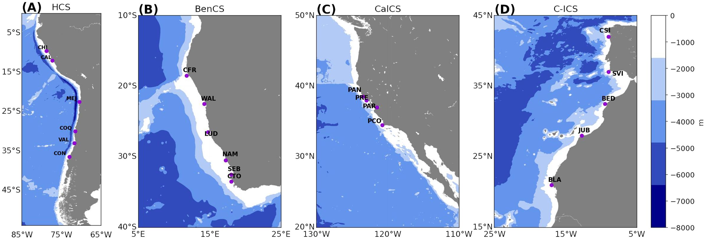
Figure 1. Geographic locations and bathymetry for the four EBUS considered in this study: (A) Humboldt (HumCS), (B) Benguela (BenCS), (C) California (CanCS), (D) Canary-Iberian (C-ICS). Bathymetry data retrieved from GEBCO (Dorschel et al., 2022).

Since these systems span wide latitudinal ranges, they are spatially heterogeneous environments (Kämpf and Chapman, 2016). At higher latitudes (25-40°N/S), upwelling is characterized by a marked seasonal cycle beginning in spring and extending through summer and early fall, with dominant downwelling-favorable winds in winter. The length of the upwelling season increases as latitude decreases, becoming a year-round process in tropical and subtropical latitudes (0-23.5°N/S) (García-Reyes et al., 2015; Wang et al., 2015).

To better understand and quantify upwelling variability within each EBUS, we selected the most recognized upwelling centers from the literature for each system based on productivity and coastal upwelling intensity, following Kämpf and Chapman (2016). For the HumCS, we chose Chimbote (CHI), Callao (CAL) Mejillones (MEJ), Coquimbo (COQ), Valparaíso (VAL), and Concepción (CON). For the BenCS, we selected Cape Frio (CFR), Walvis Bay (WAL), Luderitz (LUD), Namaqualand (NAM), Santa Elena Bay (SEB), and Cape Town (CTO). For the CalCS, we chose Point. Conception (PCO), Point. Año Nuevo (PAN), Point. Reyes (PRE), and Point. Arena (PAR). Finally, for the C-ICS we selected Cape Blanc (BLA), Cape Juby (JUB), Beddouza (BED), Saint Vincent (SVI), and Cabos Silleira (CSI). The main features of these upwelling centers are shown in Table 1.

Table 1

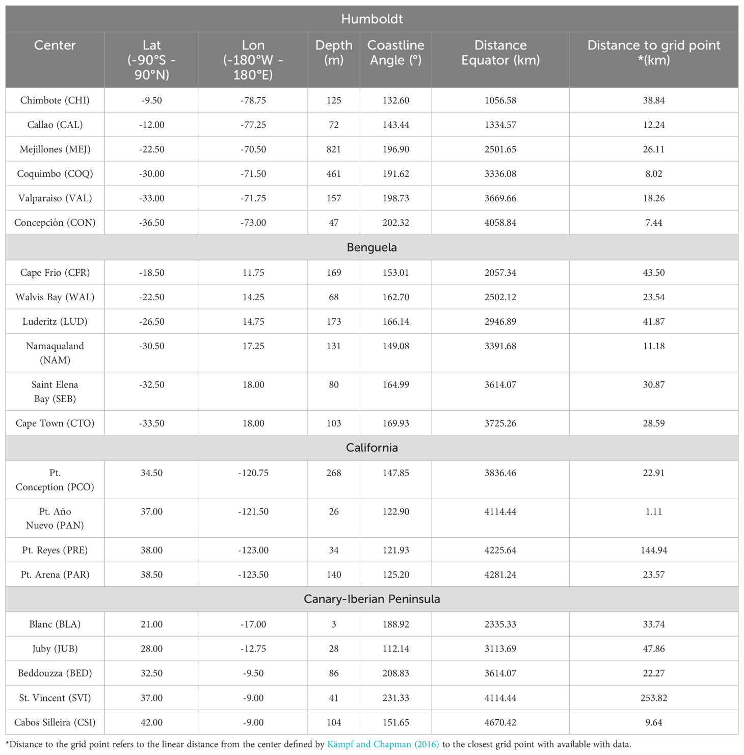
Table 1. Upwelling centers characterized in terms of their Location, Depth, Coastline orientation, Distance to the Equator and Distance to grid point.

2.2 Data sources and processing

Oceanographic and atmospheric data were obtained from various sources, including in situ observations, model simulations, and reanalysis products. An exhaustive description of the data used is presented in Table 2. Additionally, the meridional and zonal components of Ekman transport (Ev, Et), as well as Ekman pumping (Ep), were derived from the wind time series using Equations 1-3 as follows (cf. Ekman, 1905; Jacox et al., 2018; Stewart, 2008):

Table 2

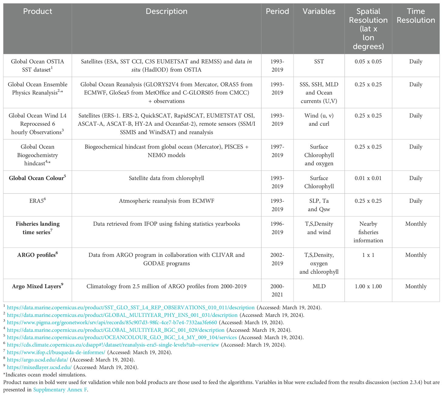
Table 2. Data sources and details on the variables used for this study.

$\begin{array}{ll}{E}_v=\frac{-{\tau }_o^x}{{\rho }_{o}f}& (1)\end{array}$

$\begin{array}{ll}{E}_t=\frac{{\tau }_o^y}{{\rho }_{o}f}& (2)\end{array}$

$\begin{array}{ll}{E}_p=\frac{1}{{\rho }_{DE}f}\left(\frac{\partial {\tau }_o^y}{\partial x}-\frac{\partial {\tau }_o^x}{\partial y}\right)+\frac{\beta {\tau }_o^x}{\rho f^2}& (3)\end{array}$

Where f is the Coriolis parameter, ${\rho }_o$ is a reference density, $\beta$ is the Coriolis parameter gradient, which is negligible since latitudinal variations are not significant. The wind stress in the eastward and northward directions are represented by ${\tau }^x$ and ${\tau }^y$, respectively. The wind curl is $\frac{\partial {\tau }_o^y}{\partial x}-\frac{\partial {\tau }_o^x}{\partial y}$ and, ${\rho }_{DE}$ represents the density at the base of the Ekman layer, obtained using Equation A16 (Supplementary Annex A).

Since spatial resolution varies among products, from 0.01 to 0.25 degrees (Table 2), all products were interpolated to a regular 0.25°x 0.25° grid using a conservative normalized method (Hill et al., 2004; Chen et al., 2016) to avoid shifting and sharp gradient issues, thereby ensuring conformity to a standardized reference grid. This method has been proven to uphold maximum and minimum values, maintaining the integrity of range and central tendency metrics (Hurrell et al., 2013), and is guaranteed to preserve the synoptic (2-6 days) and spatial scales (25-100km) of coastal upwelling (Aguirre et al., 2019).

Ocean model simulations (* in Table 2) were validated within the top 500m at seasonal scale using data from ARGO profiles. Temperature and salinity simulations in each upwelling system were compared to ARGO data using Taylor diagrams. Besides, oxygen and chlorophyll simulations were validated using data from ARGO’s biogeochemical profiles using data from the top 300m for oxygen, and using Ocean Global Colour satellite products for 1997-2019 in the case of chlorophyll (Groom et al., 2019). Additionally, data from oceanographic cruises conducted by IFOP (Instituto de Fomento Pesquero, Chile) were used for validations nearshore where ARGO profiles are scarce. The validation was conducted for all products, including satellite data (sea surface temperature, sea surface height, chlorophyll) and model outcomes (oxygen and chlorophyll), therefore there is no redundancy in assessment. Detailed results of this validation can be found at https://github.com/dfbustosus/Validation_EBUS_DavidBU (Supplementary Table B1 Supplementary Annex B).

For the following analysis we selected 15 variables: surface meridional and zonal wind (Mw always positive equatorward and Zw, respectively), sea level pressure (SLP), air temperature (Ta), shortwave radiation (Qsw), surface currents (u,v), sea surface temperature (SST), sea surface salinity (SSS), sea surface oxygen (SSO), sea surface chlorophyll (SSC), sea surface height (SSH), mixed layer depth (MLD), wind stress magnitude and wind curl. These variables were selected based on previous studies analyzing long-term variations in the circulation in in EBUS both in terms of physical (e.g., Bograd et al., 2023; Wang et al., 2015; Rykaczewski et al., 2015; Aguirre et al., 2012; Alvarez et al., 2008) and biological (Chavez and Messié, 2009; Andrews and Hutchings, 1980) conditions.

2.3 Data analysis

2.3.1 Identification of upwelling events

One of the distinctive features of EBUS oceanic and atmospheric circulation is its variability spanning periods from one day to several months. This variability is characterized by the occurrence of short-lived upwelling events with a marked seasonality. Changes in environmental forcings within EBUS lead to variations in this high-frequency variability, which motivates the analysis in the context of our study. Although there are different ways to identify upwelling events such as cross-shore SST differences (Benazzouz et al., 2014) and the vertical water transport rate along the coastline (CUTI) (Jacox et al., 2018; Bograd et al., 2023). All existing indices consider three important factors: SST, wind speed and the relative alignment of wind direction respect the coastline. Thus, these factors were used as key indicators to identify upwelling events through the upwelling index proposed by Fielding and Davis (1989):

$\begin{array}{ll}UI=\mu (\text{cos}(\theta -\alpha ))& (4)\end{array}$

Where μ and θ represent the wind speed (ms^-1) and direction (degrees), and α indicates the coastline orientation relative to the north. An upwelling event was identified based on three criteria: (1) UI > 0, (2) SST below a 25^th percentile threshold (Schlegel and Smit, 2018) using the SST daily climatology for each season, and (3) persistence of these conditions for more than 3 consecutive days. Different upwelling metrics were obtained for each system, including frequency of occurrence (Events/km²), mean intensity and duration. Frequency of occurrence indicates the number of events occurring per grid point, calculated by dividing the total number of events by the spatial extent in km². Mean intensity refers to the average temperature drop relative to the daily climatological baseline during an upwelling event, while duration measures the span in days of an upwelling event (Abrahams et al., 2021). Figure 2 illustrates an example for the HumCS.

Figure 2

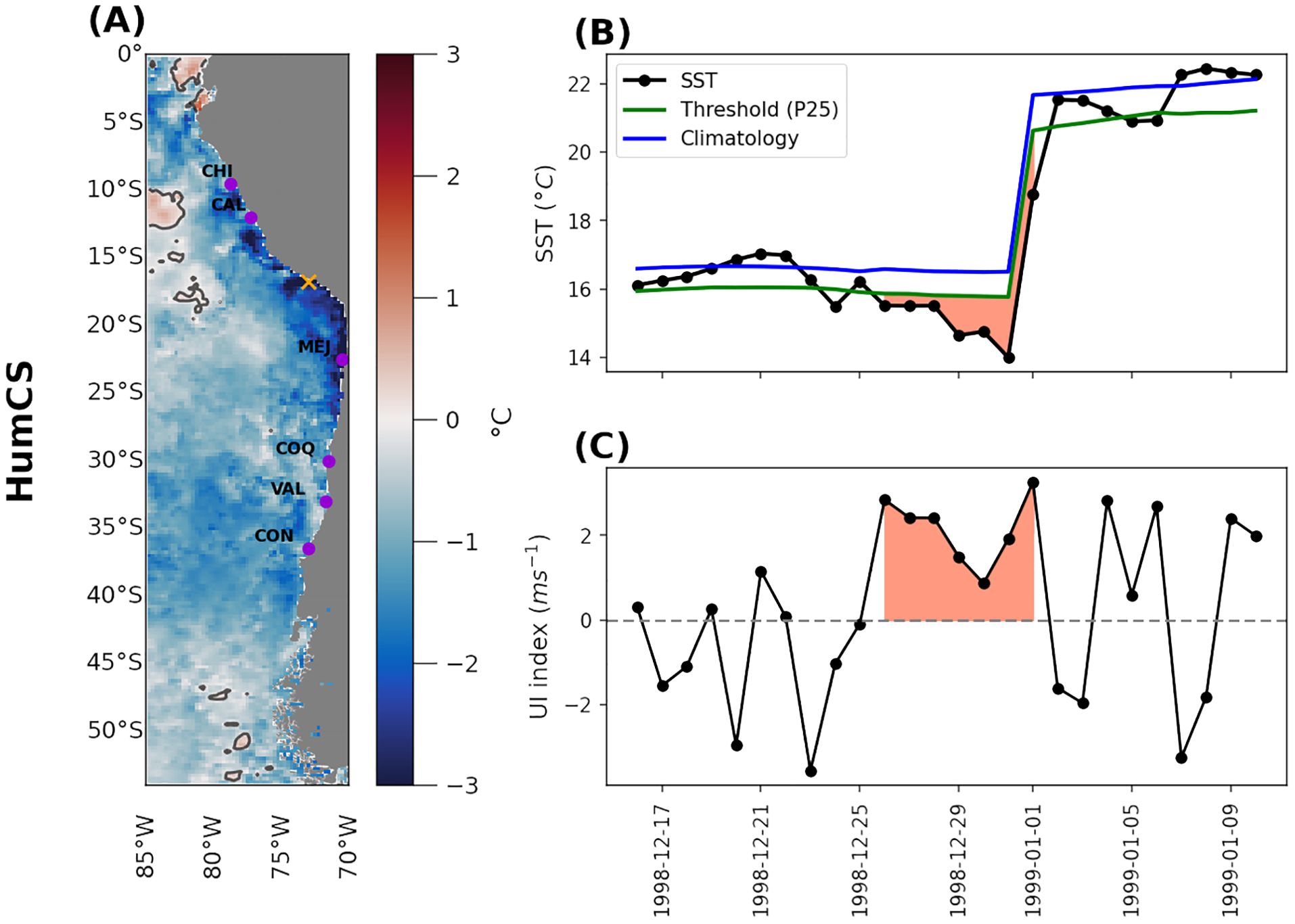
Figure 2. Upwelling events identification method for node at 73°W, 16.5°S (yellow cross in a). (A) represents the peak SST anomaly (°C) during an upwelling event spanning 23-31 December 1998. The second column (B) displays the SST time series (black), SST climatology (blue), and 25th percentile threshold (green) during the event. (C) Upwelling Index (UI) computed with Equation 4. Red shading marks the duration of the identified upwelling event.

2.3.2 Self-organized map

The SOM is an Artificial Intelligence technique based on competitive learning (Kohonen and Somervuo, 1998; Vesanto and Alhoniemi, 2000) that has found application in oceanographic and atmospheric studies (e.g., Le Bars et al., 2016; Sonnewald et al., 2021) to characterize circulation patterns resulting from non-linear processes in multidimensional data (Qian et al., 2016). This method offers distinct advantages over linear approaches such as EOFs (North, 1984) and K-means (Dreyfus et al., 2005) for three primary reasons: first, it handles non-linearities inherent in biophysical processes not assuming normal data distributions; second, it preserves topology to maintain spatial relationships; and third, demonstrates robustness to outliers (Liu and Weisberg, 2011). Despite these advantages, however, the application of this technique to analyze the dynamics of upwelling within EBUS over an extended period remains unexplored.

The SOM is used to obtain the main patterns of spatial variability (i.e. clusters) within each EBUS separately, along with the dates of upwelling events. For this purpose, we selected 15 variables (Section 2.3.1) considering solely unique dates when upwelling events occurring in any of the nodes along the coast for each EBUS by two reasons: first, upwelling events are the primary focus, and second, incorporating other data would introduce noise into the algorithm’s learning. Figure 3 provides a schematic overview of the multivariate SOM technique. All the data (k) for each time (t) are flattened into vectors (x_t) that contain only ocean nodes. These vectors form a 2D array, which is used first to find the best network configuration (rectangular 2-D maps, which represents the optimal configuration for the model’s learning process) and second to update the weights (W) of the SOM neural network with competitive learning. The best network configuration (2-D map neurons, Figure 3) ensures an efficient learning process (see Supplementary Annex C Supplementary Figure S1). This optimal configuration is identified using two metrics following Jebri et al. (2022): the quantization error (QE) and topological error (TE). While QE provides a reliable indicator of potentially critical changes in spatial structure over time (Sun, 2000), TE allows quantifying geometric preservation of the dominant structures, which implies understanding the quality of the map’s representation and organization of the input data (Gibson et al., 2017). These two metrics are widely used to validate the performance of the SOM algorithm (Liu et al., 2006; Naik and Shah, 2014).

Figure 3

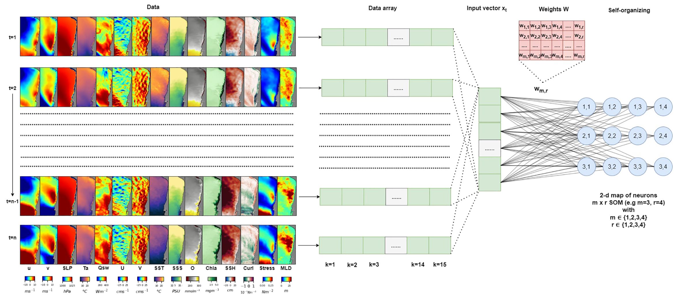
Figure 3. Schematic of the SOM technique adapted from Liu and Weisberg (2011). The 3-D data time series (lat,lon,time) for each variable (k) (left panel) are rearranged in a 2D array that includes all variables considered, where each time step is reshaped as a row vector (x_t) (middle panel, Data array). For each time step (t), the row vector is used to update the weights (W) of the SOM network with competitive learning. The iterative process is also known as self-organizing (Right panel, Self-organizing). The outcome clusters from SOM neurons (blue circles) are reshaped back into characteristic patterns. Each neuron contains different instances with similar variability, basal structure, etc., and these can be associated as clusters of data.

During the learning process the algorithm weights are calibrated based on QE and TE metrics. The SOM outputs an mxr list of clusters, each containing times associated with similar spatio-temporal variability. These clusters are reshaped back into characteristic patterns by averaging maps for all times associated to the cluster. These patterns reveal dynamic signals of dominant upwelling behavior, distinct from those derived from mean nor linear trend analyses, which are often smooth masking the large variability in the process of interest (Kohonen and Somervuo, 1998; Jouini et al., 2016), potentially offering new insights into circulation changes. Further details on SOM parametrization are provided in Supplementary Material, Supplementary Annex C (Supplementary Table C1).

2.3.3 Hierarchical clustering algorithm

The SOM algorithm yields between 12 and 16 spatial patterns of variability, many of which exhibit similar spatial structure. To simplify these results and derive the final spatial patterns for each EBUS, we implemented the Hierarchical Clustering Algorithm (HAC) technique (Jain et al., 1999). HAC is an unsupervised machine learning method known for its ability to uncover patterns and relationships within complex datasets (Saraceno et al., 2006; Li et al., 2020; Liu et al., 2021). This technique clusters data based on similarities and dissimilarities using a distance metric and grouping criterion.

We applied HAC to reduce the number of clusters generated by the SOM, resulting in the final patterns of variability. Similarity between objects was assessed using the Euclidean distance metric (Nielsen and Nielsen, 2016) and clustering was performed based on the Ward criterion (Murtagh and Legendre, 2014). The dendrogram helped identify a small number of cohesive groups. Figure 4 illustrates the integration of SOM and HAC. For each resultant cluster, we counted the number of associated days, yielding the number of days with upwelling events related to this pattern (section 3.1). Subsequently, temporal averages are computed to obtain the mean spatial structure linked to each cluster (section 3.2). These averages can be calculated for the entire period or for shorter intervals (see section 2.3.4) to observe the evolution of spatial structures (sections 3.3 and 3.4).

Figure 4

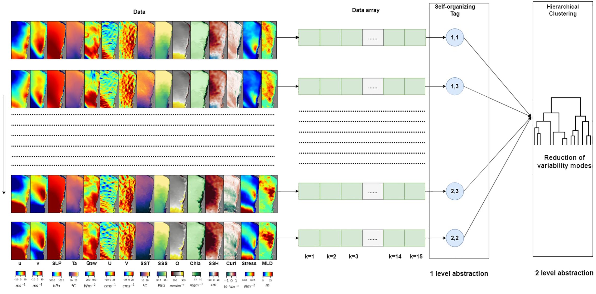
Figure 4. Illustration of two-level abstraction clustering algorithm SOM - Hierarchical Clustering. Daily tag/cluster results from multivariate SOM (see Figure 3) are used to provide the input (middle panels, Self-organizing Tag) to the second level of abstraction level using the clustering technique (right panel, Hierarchical Clustering (HAC).

2.3.4 Long-term analysis

Yearly time series spanning from 1993 to 2019 were constructed for the number of days with upwelling occurrences, derived from the principal spatio-temporal patterns of variability obtained for each EBUS and season (i.e., spring and summer). This approach allows for comparison of the variability explained by each pattern. Spatial averages of SLP, meridional wind component (Mw), Qsw, SST, and Ep were calculated from the dominant spatial pattern (see Section 2.2). These averages help identify similarities and differences across each EBUS and season analyzed.

Certain variables (highlighted in blue, Table 2) were excluded from the primary analysis but are presented in Supplementary Annex F due to the following reasons. First, surface chlorophyll and oxygen were omitted due to incomplete representation nearshore accuracy in the hindcast product (Fransner et al., 2020). Secondly, wind stress and curl are used for Ek and Ep calculations respectively (Section 2.2), SSS lacks notable variability, and its exclusion makes it possible to avert Simpson’s paradox in the analysis (Wagner, 1982). Ocean currents were not included as they derive from atmospheric and ocean factors already included in the analysis. Finally, SSH was omitted to prevent redundancy, as it reflects the influence of atmospheric pressure, surface wind, SST, and SSS (Stewart, 2008). However, all variables are included because this approach, unlike multivariate techniques such as EOFs, accounts for nonlinear interactions between variables. This method had shown benefits in providing a more accurate representation of highly variable systems (Lachkar and Gruber, 2012; Nakaoka et al., 2013). Nonetheless, its implementation in other studies has been focused narrowly on discerning patterns within a limited subset of variables (Richardson et al., 2003; Liu and Weisberg, 2011).

To quantify the long-term changes of the dominant spatial patterns obtained for each EBUS, we compared approximately two different decades by dividing the time period in past changes (1993-2006) and relatively new changes (2007-2019), based on the data availability. Spatial anomalies, computed by contrasting these two periods, were used to assess the magnitude of variations using SLP, the meridional wind component, Qsw, SST, zonal Ekman transport (Ek), mixed layer depth (MLD), and Ep.

Furthermore, to assess long term temporal changes in specific areas with strong upwelling, i.e., upwelling centers (Table 1), we conducted paired t-tests with Bonferroni correction using the dominant spatial pattern and the two selected periods (1993-2006 and 2007-2019). The Bonferroni correction (Perneger, 1998) adjusts the significance level of hypothesis tests to account for multiple comparisons simultaneously, thereby reducing the risk of false positives (Type I error) by setting a stricter p-value threshold for each individual test (Napierala, 2012). A significance level of 5% was applied. This approach allows quantification of the extent of change in each center, while controlling for potential confounding effects of the unique geographical location and physical conditions at each site. By accounting for these differences, the t-statistic enables isolation and fair comparison of variability magnitude. Selected variables such as SST, Mw, QST and Ep were used in the comparisons. Additionally, Pressure Gradient (PG) and Temperature Gradient (TG) were calculated as differences between the closest three ocean-to-land grid points at each latitude following the methodology proposed by Jacox et al. (2018) to test the Bakun hypothesis. Mixed-layer depth was also included in the analysis to assess potential changes in the oceanic vertical structure.

2.3.5 Subtropical high detection center

To assess the role of latitudinal shifts in the subtropical-high systems (SPHS), we identified and tracked the centers of subtropical highs in EBUS, the North Pacific Subtropical High (NPSH), North Atlantic Subtropical High (NASH), South Pacific Subtropical High (SPSH), and South Atlantic Subtropical High (SASH). The geographic limits considered were: NPSH (25-45°N, 180°E- 130°W), NASH (25-45°N, 70-20°W) from Song et al. (2018), SPSH (15-50°S, 150-69°W) based on Ancapichún and Garcés-Vargas (2015), and SASH (20-40°S, 42°W-12°E) as described by Reboita et al. (2019).

Two versions of an eight-step algorithm to identify subtropical-high centers were applied (see Supplementary Annex D for more details). The first algorithm, described by Gilliland and Keim (2018) and the second algorithm, described by Lambert (1988 and Murray and Simmonds (1991). The second algorithm addresses issues related to disturbances caused by transient weather systems and offers robustness against the potential fragmentation of subtropical highs by cold fronts and anticyclones, particularly when daily data are used to locate the center (Degola, 2013). Results from algorithm 1 (Supplementary Material Table D1) were used to determine the daily position of subtropical highs, associating them with various spatial patterns of variability identified by the SOM algorithm. Additionally, results from algorithm 2 (Supplementary Material Table D2) were used to investigate decadal trends in the movement of each subtropical high center (results not shown).

3 Results

This section begins detailing the number of days with upwelling events within the primary variability patterns. Therefore, describes the principal spatial pattern for each EBUS, followed by an analysis of how these patterns evolve over time. Finally, summary statistics, including various upwelling metrics, are provided to facilitate comparison across the different EBUS.

3.1 Number of days with upwelling events in the main variability patterns

The principal spatial pattern of variability derived from the SOM-HAC algorithm characterizes the upwelling regime, revealing the predominant signal within each season and EBUS. The results demonstrate a distinct separation among the dominant spatial pattern of variability (depicted by blue lines in Figure 5), with prevalence exceeding 56% across all EBUS. The mean number of days with upwelling per year and season (denoted as $\overline{X}$ in Figure 5, resulting from adding the blue, red, and green lines) shows higher values during spring (Figures 5A–D) compared to summer (Figures 5E, F), ranging from 50.4 days yr^-1 (Figure 5H) to 83.6 days yr^-1 (Figure 5A). The CalCS and HumCS exhibit the highest number of days with upwelling events per year, with HumCS recording the highest number (83.59 days yr^-1). No significant linear trends were observed at the inter-annual scale for either spring or summer.

Figure 5

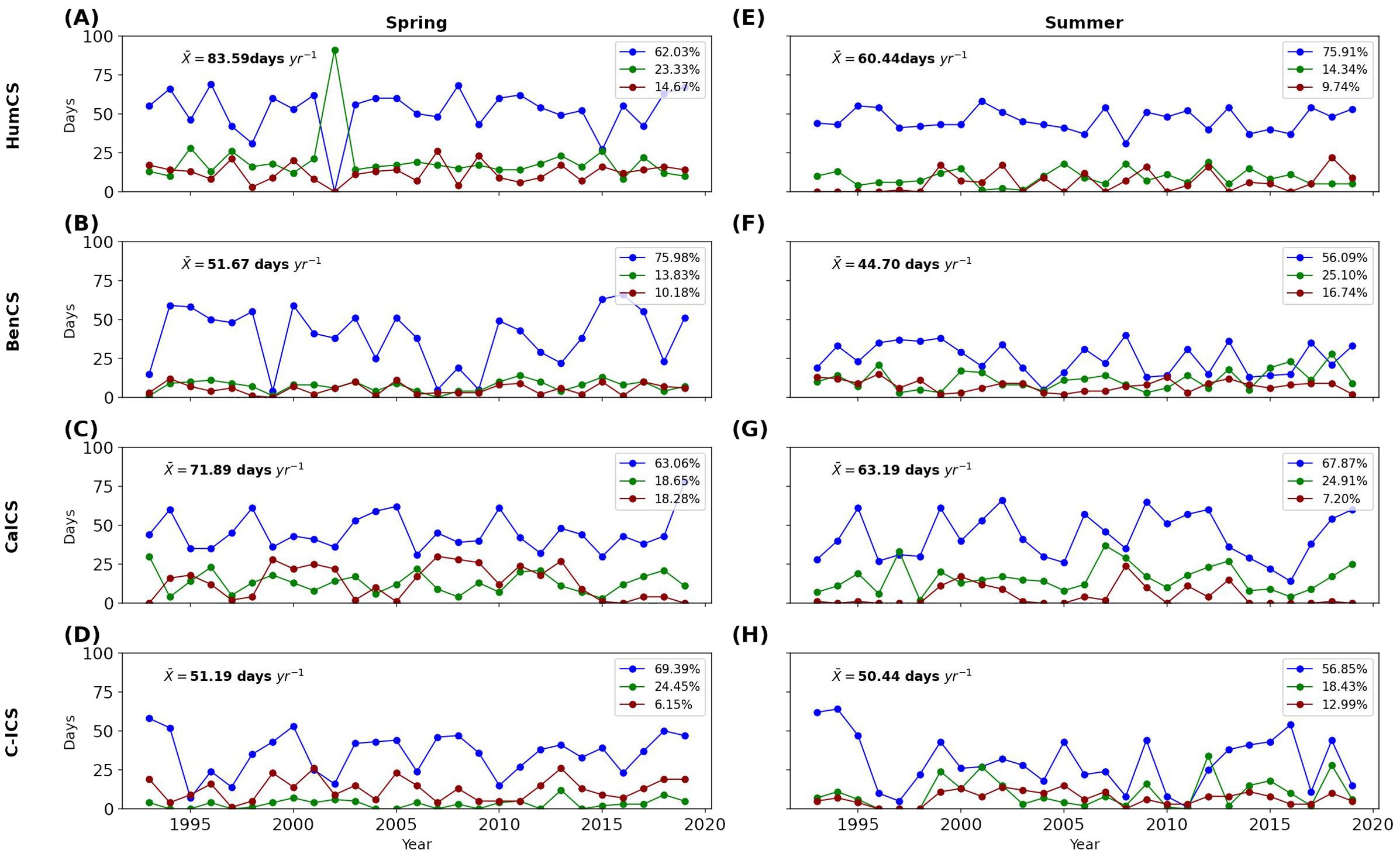
Figure 5. Time series of the annual upwelling duration (in days, this represents how many distinct dates where under upwelling events for a given season, spring (A-D) and summer (E-H)) of the main three dominant spatial patterns detected by SOM-HAC algorithm for each EBUS and season (spring (left) and summer (right)). The y-axis represents the duration (days), and the x-axis represents the years. The first spatial pattern (blue), second (green), and the third (red) presented in decreasing order of occurrence. Mean numbers of days with upwelling per year ($\overline{X}$) are reported in upper left corner of each panel. Legends show the percentages of the total variance explained by each spatial pattern.

3.2 Spatial structure of SOM dominant spatial pattern

Using the dates associated with the dominant spatial pattern (selecting spatial pattern-specific dates and averaging them), we reconstructed the spatial structure of the key variables relevant for understanding changes in the ocean and atmospheric circulation within these coastal upwelling systems. There variables were SLP, Mw, Qsw, SST and Ep (Figures 6, 7). Interestingly the dominant spatial pattern captures the seasonal cycle across all EBUS, which is clearly evidenced by the presence of the Coastal Jets (Mw) and the subtropical anticyclones (SLP). This is noteworthy given that the input data only includes short-lived upwelling events. It suggests that the marked seasonality in intraseasonal variability within EBUS systems is driven by upwelling-favorable winds due to extratropical disturbances and seasonal changes in oceanic mixing (e.g. Renault et al. (2009) for HumCS, Goubanova et al. (2013) for BenCS).

Figure 6

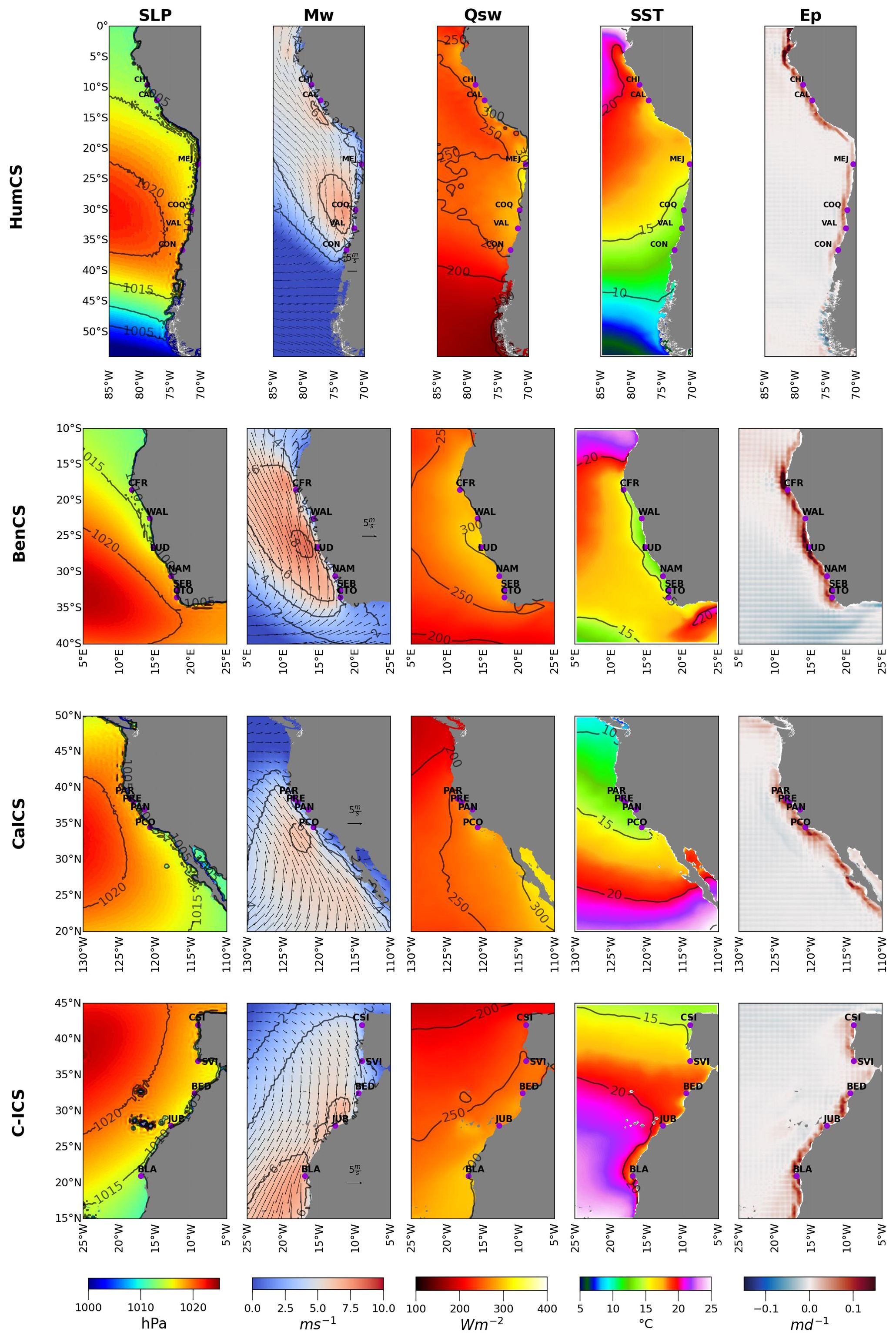
Figure 6. Spatial structure for the dominant spatial pattern of variability during spring, visualized as dominant patterns in SLP (sea-level pressure), Mw (meridional wind), Qsw (shortwave radiation), SST (sea-surface temperature), and Ep (Ekman pumping) during periods when upwelling occurred. These variables are organized in columns, whereas the four rows of plots correspond to the EBUS regions analyzed.

Figure 7

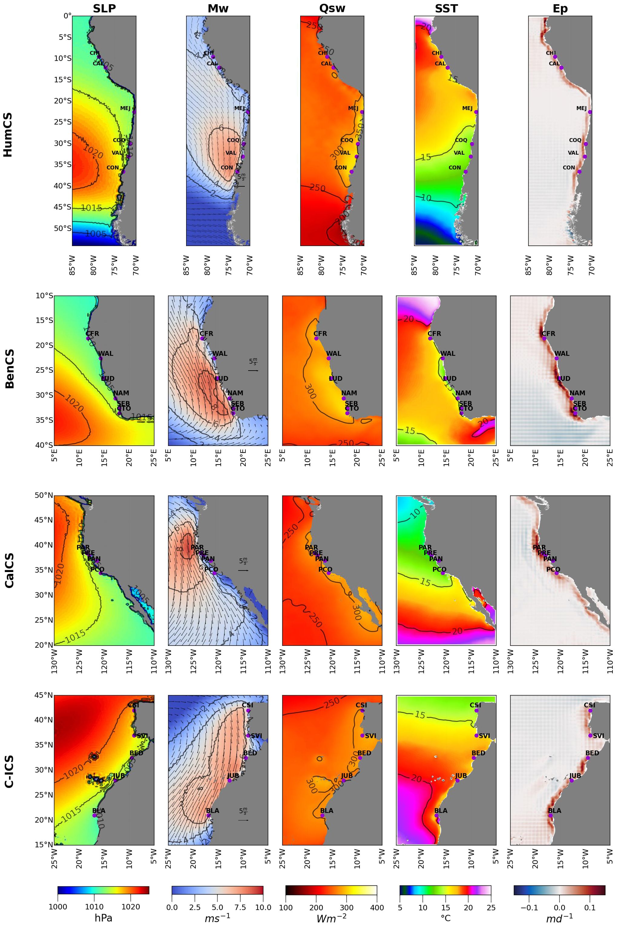
Figure 7. Same as Figure 6 but for summer.

In the spring season (Figure 6), significant SLP isobars exceeding 1020 hPa are observed near the coast and displaced polewards in CalCS, C-ICS and BenCS. The meridional wind component (Mw) exhibits higher values in the mid-latitude regions and towards the poles across most of the systems, with particularly elevated values in BenCS and CalCS (> 8 m s^-1). Shortwave radiation (Qsw) ranges between 200 and 300 Wm^-2 across all upwelling centers, with higher values in BenCS (up to 300 Wm^-2). Sea surface temperature (SST) drops below 15°C nearshore in the major upwelling centers along HumCS, BenCS and CalCS. Conversely, C-ICS shows higher SST values (15-20°C) throughout the region. The Ekman pumping (Ep) displays an increasing trend nearshore with values exceeding 0.1 md^-1 at the most significant upwelling centers.

In the summer season (Figure 7), the spatial distribution of SLP exhibited a similar pattern to spring, with the 1020 hPa isobar situated closer to shore in CalCS and C-ICS compared to HumCS and BenCS. As expected for summer, there was a notable increase in the meridional wind (Mw) (> 6ms^-1) from mid-latitude and toward the poles across all EBUS. SST and Ep, displayed spatial patterns similar to those observed int the spring season (Figures 6, 7).

We do not present the second and third spatial patterns of variability as each contribute less than<50% of the total variability for each system and season considered. However, a detailed description of these spatial patterns of variability is presented in Supplementary Annex E, Supplementary Material (Supplementary Figures S5-S8).

3.3 Spatiotemporal changes in the dominant spatial pattern of variability

When comparing the decadal changes in the principal spatial pattern of variability, mid-latitude regions in all EBUS showed an increase in SLP ranging between 0.2 and 0.8 hPa (Figure 8, positive anomalies SLP column). The centers of all subtropical highs (SPHs) exhibited a poleward displacement ranging from 89 and 224 km, accompanied by a slight offshore shift, except for CalCS (Table 3. Supplementary Annex C, Supplementary Figure S2). There was a noticeable increase in the meridional wind component (Mw) ranging from 0.5 to 1 ms^-1 (Figure 8, Mw column) in CalCS and C-ICS toward the poles. In HumCS and BenCS, Mw showed slight increases in opposite directions: HumCS with a more pronounced trend at lower latitudes, excluding regions around 15-20°S and near 40°S, while BenCS, the trend was poleward of 20°N. Qsw increased up to 5 Wm^-2 in BenCS, CalCS, and C-ICS, especially nearshore. Conversely, HumCS experienced a reduction in Qsw across the entire system ranging from 5 to 10 Wm^-2 (Figure 8, Qsw column). SST displayed a decrease nearshore ranging from 0.3 to 0.6°C in middle and higher latitudes, except in C-ICS and BenCS where an increase between 0.2 and 0.4°C was observed. HumCS showed a significant northward increase (>1°C) northward from 25°S, consistent with the reduction in Mw (Figure 8, SST column). Moreover, there was a reduction in Ep nearshore for all EBUS, except for HumCS, where Ep increased (Figure 8, Ep column).

Figure 8

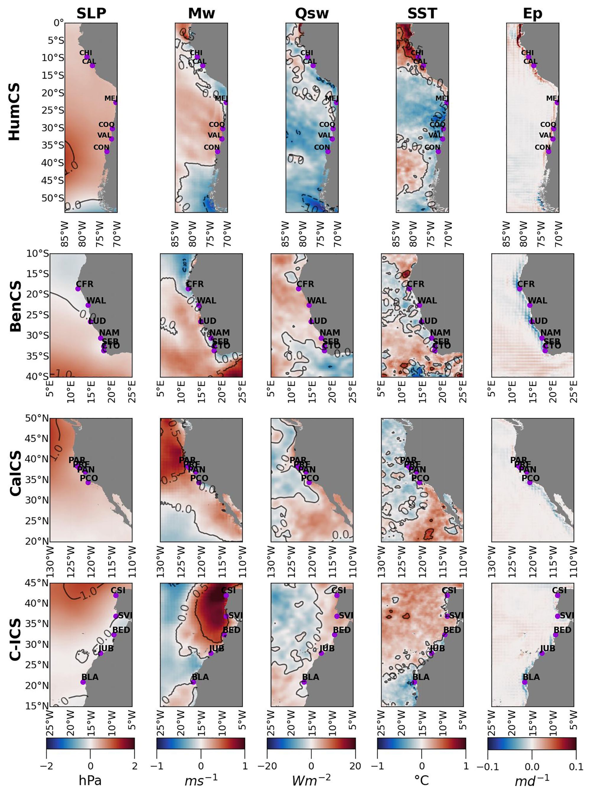
Figure 8. Spatial pattern of temporal changes (2007-2019 minus 1993-2006) in the dominant spatial pattern of variability for spring (Figure 5, left column) reflected in the variables sea-level pressure (SLP), meridional wind (Mw), short-wave radiation (Qsw), sea-surface temperature (SST), and Ekman pumping (Ep). Each row of panels corresponds to an EBUS, whereas columns denote different variables. Red values in second-column panels (Mw) indicate upwelling-favorable winds.

Table 3

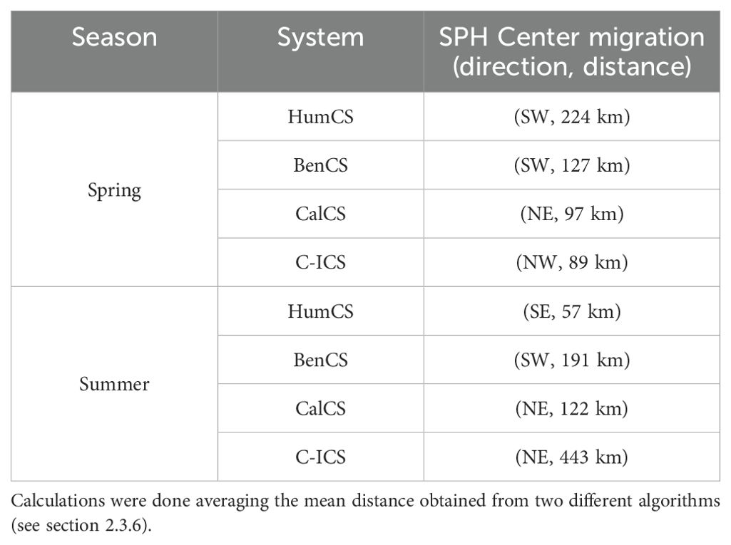
Table 3. Displacement of Subtropical-High Centers when comparing 2007-2019 with 1993-2006.

For the summer season (Figure 9), subtropical high-pressure systems exhibited a poleward (and slightly shoreward) shift, with displacements ranging between 57 and 443 km, except for BenCS, which showed a westward shift (Table 3). However, SLP increases were less pronounced compared to spring, with increments less than 0.5 hPa across all systems (Figure 9, left column). Furthermore, most systems showed an increase in meridional wind (Mw) during summer, ranging from 0.2 to 0.8 m s^-1. However, reductions were observed in CalCS and C-ICS, for instance towards BLA upwelling center. HumCS showed a different pattern with a weakening of equatorward winds ranging from 0.1 to 0.4 m s^-1 at mid-latitudes (25-35°S). In contrast to spring, Qsw decreased by 5 to 15 Wm^-2 in most systems during summer. SST patterns varied across EBUS: HumCS and CalCS showed decreases ranging between 0.1 and 0.6°C, while C-ICS and BenCS showed increases in nearshore waters ranging from 0.2 to 0.6°C. In the HumCS, SST increased (> 0.1°C) significantly northward from 25°S, consistent with the decrease in nearshore Mw. Finally, there were reductions in Ep nearshore in BenCS and CalCS, while summer Ep increased in HumCS and CanCS (Figure 9).

Figure 9

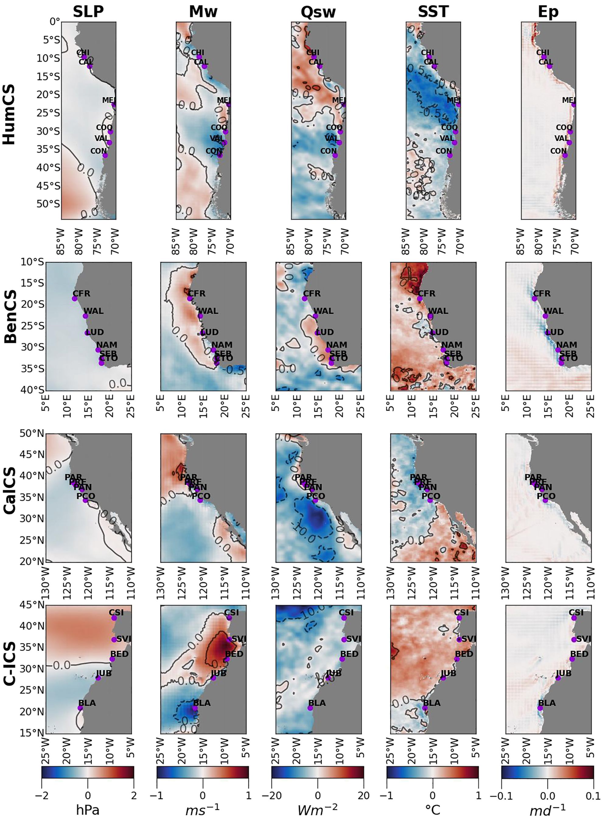
Figure 9. Same as Figure 8 for summer.

3.4 Decadal changes in the upwelling centers

In addition to the general spatial and long-term changes described above, we conducted a detailed analysis of specific areas known for strong upwelling (i.e. upwelling centers). Figure 10 presents the result of the Bonferroni multiple comparisons test, which adjusts for differences in averages and variability between the approximately two decades 2007-2019 and 1993-2006. Alongside the variables described in section 3.3: Pressure Gradient (PG), Temperature Gradient (TG), Zonal Ekman transport (Ek) and Mixed Layer Depth (MLD) were included to assess potential changes in the oceanographic vertical structure at these centers.

Figure 10

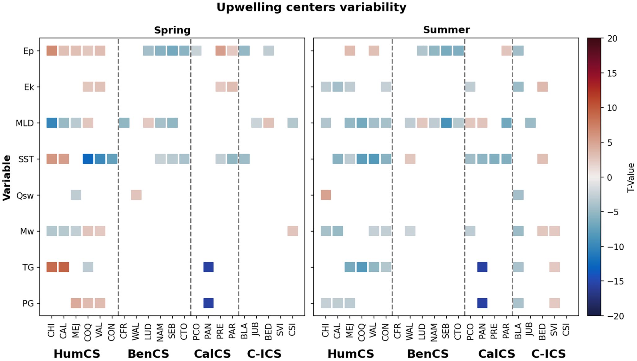
Figure 10. Measures of decadal changes at upwelling centers, from Bonferroni-corrected multiple comparison tests applied to Pressure Gradient (PG), Temperature Gradient (TG), meridional wind (Mw), short-wave radiation (Qsw), sea-surface temperature (SST), mixed-layer depth (MLD, positive means deeper MLD), zonal Ekman transport (Ek), and Ekman pumping (Ep). Colors represent the magnitude of the t-statistic and indicate increases (red) and reductions (blue) in values of the period 2007-2019 relative to 1993-2006. Only changes that were significant for alpha=0.05 are shown.

During spring, an increase in the Pressure Gradient (PG) (i.e., larger land-ocean) was observed at HumCS for upwelling centers Mejillones (MEJ), Coquimbo (COQ), and Valparaíso (VAL) (Figure 10). Conversely, in summer, there was a slight drop in PG for Chimbote (CHI), Callao (CAL), and Mejillones (MEJ) in HumCS, as well as for Blanc (BLA) in the C-ICS. Point Año Nuevo (PAN) in CalCS showed a decreasing pattern in both seasons analyzed, while no significant changes (white spaces) were observed for BenCS. Besides, a distinctive pattern emerged in HumCS where PG increased towards the south during spring, coinciding with an increase in TG towards the north. In summer, as PG decreased towards the north, TG decreased towards the south. Point Año Nuevo (PAN) in CalCS was the only upwelling center that displayed significant reductions in TG. Additionally, an opposite pattern of TG change was observed in C-ICS between Blanc (increase) and St. Vincent (decrease).

Meridional winds (Mw) decreased at most upwelling centers in the HumCS during both spring and summer, except for Coquimbo (COQ) and Valparaíso (VAL) in spring. In summer, Mw weakened notable at Chimbote (CHI) and Callao (CAL) in HumCS, Walvis Bay (WAL) in BenCS, Pt. Conception (PCO) in the CalCS, and Blanc (BLA) in the C-ICS. Conversely, Cabo Silleira (CSI) showed an opposite pattern in spring within C-ICS, while Beddouzza (BED) and St. Vincent (SVI) exhibited changes in summer. Significant drops in SST were observed at most upwelling centers, particularly those at higher latitudes, except for Walvis Bay (WAB) in BenCS, and Beddouza (BED) in C-ICS during summer. Similar patterns were observed for MLD. Zonal Ekman transport (Ek) showed increases during only in the Pacific systems, specifically at Coquimbo (COQ) and Callao (CAL) in HumCS, Point Reyes (PRE), and Point Arena (PAR) in CalCS. Conversely, Ek decreased during summer at most centers, with no significant changes observed in BenCS. Ekman pumping (Ep), increased in both spring and summer for HumCS, while higher-latitude centers in BenCS showed decreases in both seasons. In CalCS, Ep increased at Point Reyes (PER) and Point Arena (PAR) but decreased at Blanc (BLA) and Beddouzza (BED) in C-ICS.

Besides, we calculate relative changes in the seasonal cycle using Equation 5 (see Supplementary Material, Supplementary Annex C, Supplementary Figure S3). Results indicate an amplification in the seasonal cycle across the EBUS.

$\begin{array}{ll}\frac{{[Spring-Summer]}_{difference}}{{[Spring-Summer]}_{mean}}& (5)\end{array}$

3.5 Summary upwelling metrics

The SOM-HAC results are based on the days when upwelling occurs (section 2.3.1), enabling the description of the upwelling process in the EBUS using various metrics. The upwelling metrics derived for each system during the study period (events/km² affected, mean duration and intensity), reveal that HumCS experiences significant more events (Table 4), with a higher occurrence during summer (0.022) than spring (0.016). BenCS shows a similar pattern. Conversely, CalCS and C-ICS exhibit significantly more events during spring than summer (Table 4). In terms of mean duration, events last significantly longer in spring across all EBUS (One-way ANOVA, F=27.86, p<0.001, df= 3). Upwelling events persist longer in in the HumCS and CalCS, ranging from 6.8 to 8.5 days, whereas in other regions, durations do not exceed 6 days. Regarding the mean intensity of upwelling events, values are significantly higher during summer in all EBUS except C-ICS (One-way ANOVA, F=985.04, p~0, df= 3), reaching up to -1.7°C in BenCS.

Table 4

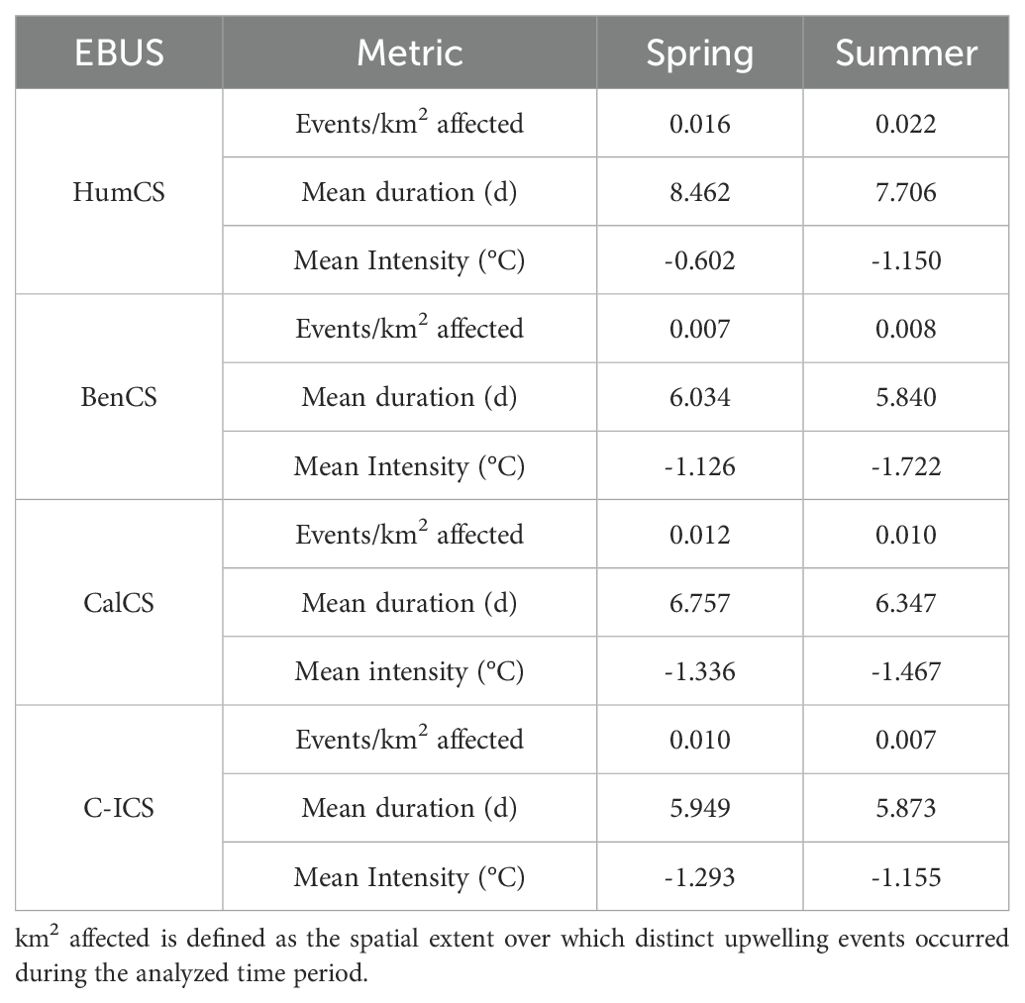
Table 4. Upwelling metrics (Events/km² affected, mean duration and intensity defined in Section 2.3.1) from events detected (Section 2.3.2) in the 1993-2019 period.

Table 5

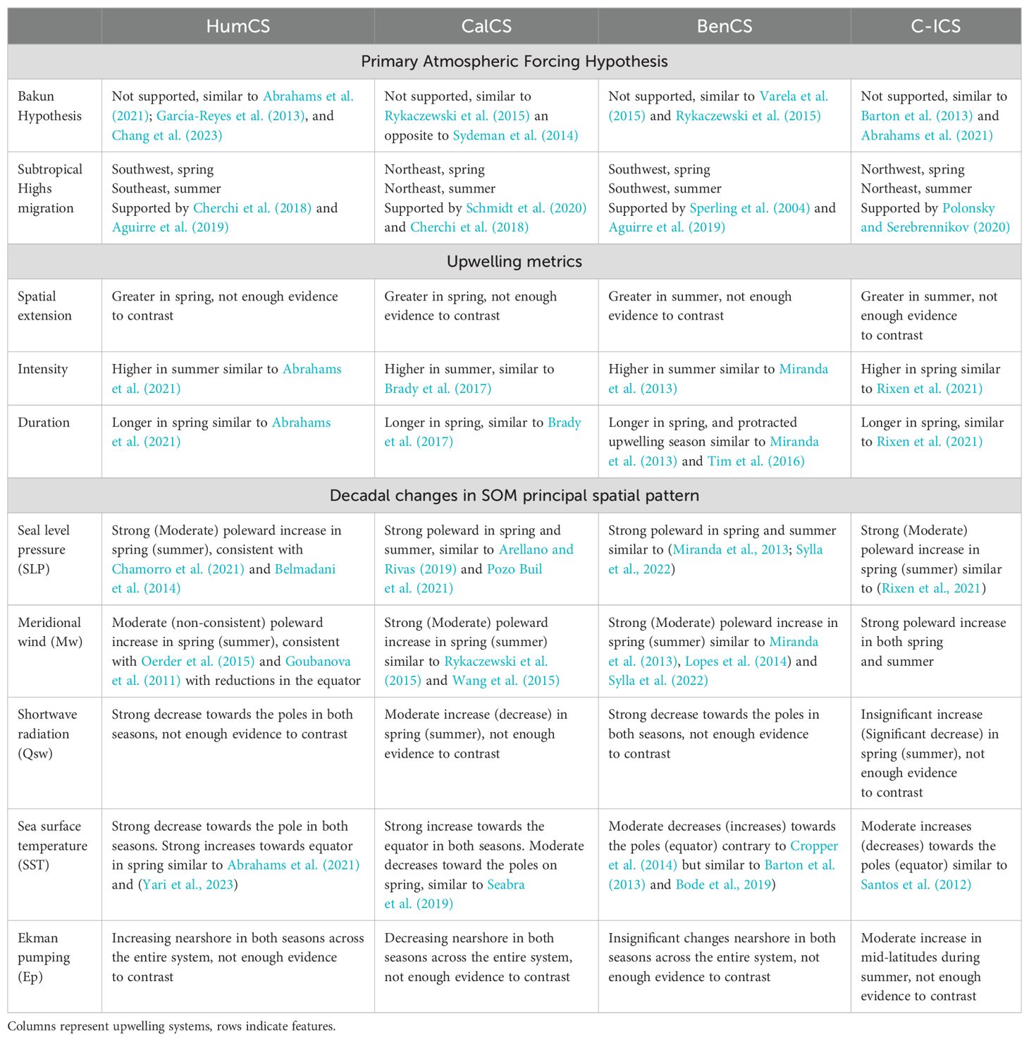
Table 5. Overview of main findings in this study with indication of discrepancies or consistency with previous studies.

4 Discussion

In this study, we utilized various metrics (frequency of occurrence, mean duration, and intensity) to characterize and compare the phenology and interannual trends of the upwelling process across major EBUS worldwide. Analysis of upwelling metrics across these regions revealed that, on average, upwelling events are longer during spring and more intense in the summer. An exception to this trend is observed in the Canary Islands region (C-ICS, Table 4), where recent observations indicate an increase in upwelling-favorable winds without significant changes in SST nor the vertical motion of coastal waters (Narayan et al., 2010; Patti et al., 2010).

We also assessed the principal spatial patterns of upwelling variability in the four major EBUS from 1993-2019 using various datasets for atmospheric and oceanic variables (Table 2). These spatial patterns were extracted using an innovative clustering technique known as SOM-HAC, focusing on periods classified as upwelling events (i.e. upwelling-favorable winds for more than three days and SST below the 25^th percentile climatological threshold). Additionally, changes in dominant spatial pattern were examined across different known upwelling centers within each EBUS.

In this study we implemented a novel approach in oceanography based on Artificial Intelligence applied to multivariate datasets (15 variables). This technique considers the nonlinear interactions that may be linked to climate change in the main EBUS. Through this approach, we aimed to expand our understanding of the complexities underlying coastal upwelling processes and their response to climate-driven changes in atmospheric and oceanographic forcing. While our findings align with previous studies, they also reveal new insights into the variability of upwelling in these regions.

The method yields a main spatial pattern of variability that accounts for the seasonality in the circulation in the EBUS. During spring, the most prominent signal in EBUS is characterized by a poleward displacement of subtropical high-pressure systems, accompanied by stronger equatorward winds in the mid to high latitudes for some regions. This is associated with higher shortwave radiation, lower SST, and consistent increases in Ekman pumping nearshore. Similar conditions are observed during summer, with stronger winds in mid-latitude regions, lower SST nearshore, increased Qsw and similar Ep values. The principal spatial pattern of variability resembles the differences between spring and summer, especially in terms of sea level pressure (SLP) and the meridional wind (Mw) (see Figures 6, 7). Despite the similarity among EBUS in terms of physical drivers for coastal upwelling, the specific responses can vary among regions. For instance, mid-latitude SST in Benguela rises from spring to summer (Figures 6, 7), consistent with previously reports results (García-Reyes et al., 2023), attributed to the impact of anticyclone intensity on lower-latitude sections of the Benguela system (Bordbar et al., 2023). Mahlobo et al. (2024) suggest that the change in intensity at the equator and consequent reduction in the wind-stress-curl-driven is decreasing due to the migration of the South Atlantic Subtropical High (SASH). Another notable difference among regions is the much greater surface area with meridional winds above 6 ms^-1 at BenCS and C-ICS, especially in mid-latitude regions and towards the poles, contrasting with the more focalized increases in Mw at HumCS (30-40°S) and CalCS (35-45°N).

In recent decades studies focused on the C-ICS have indicated a rise in SST attributed to a weakening or reversal of the trade winds (Vallis, 1986; Saji et al., 1999; Sambe et al., 2016). Our findings confirm this warming trend, particularly evident in the first principal spatial pattern of variability from the SOM, showing a substantial increase in both spring and summer (Figures 8, 9). However, distinctive patterns emerge in the second and third spatial patterns of variability, particularly in BenCS and C-ICS (see Supplementary Annex E).

We found that the area affected by upwelling in Southern Hemisphere systems is larger in summer than in spring, which contrasts with the pattern observed for the Northern Hemisphere systems (see Table 4). The occurrence of shorter and more intense upwelling events in spring (Table 4) aligns with the findings of Abrahams et al. (2021), despite differences in the spatial scope of the datasets used. Our study encompasses a broader dataset, extending beyond the coast. Other studies also support the idea that more upwelling events occur in spring. For instance, Miranda et al. (2013) and Tim et al. (2016) found more frequent high-intensity upwelling events from spring to summer in CalCS and C-ICS, similar to our results.

Our results showed no evidence supporting the Bakun hypothesis (Bakun, 1990) across EBUS upwelling centers, indicating an absence of consistent changes in ocean-land pressure or temperature gradients (see Figure 10). Similar findings have been reported in others studies (Rykaczewski et al., 2015; Abrahams et al., 2021; Chang et al., 2023). One possible explanation for this lack of support for Bakun’s hypothesis is the absence of deepening in the continental thermal low-pressure systems (CTLPS) with increasing temperatures (Rykaczewski et al., 2015; Chamorro et al., 2021). Additionally, observations from recent decades (Sydeman et al., 2014), and evidence that winds in the EBUS are driven mainly by the position and intensity of the subtropical high-pressure system (SHPS) (García-Reyes et al., 2013; Schroeder et al., 2013; Flores-Aqueveque et al., 2020; Yang et al., 2022), suggest that wind intensity trends might be more sensitive to the poleward migration of the SHPS rather than to changes in the CTLPS (Bakun et al., 2015; Belmadani et al., 2014; Garreaud and Falvey, 2009; Rykaczewski et al., 2015). Thus, the best explanation for the large-scale changes observed in these systems is the poleward displacement of the SHPS, driven by the expansion of Hadley Cells due to increased warming rates over the tropics relative to the equator. Our results show that the SHPS centers have indeed migrated poleward during spring and summer (Figures 8, 9, Table 3, Supplementary Material Figure S2), except for BenCS. This is consistent with previous studies on the HumCS (Ancapichún and Garcés-Vargas, 2015; Flores-Aqueveque et al., 2020; Weidberg et al., 2020), BenCS (Gilliland and Keim, 2018; Reboita et al., 2019), CalCS (Riyu, 2002; Song et al., 2018), and C-ICS (Yang et al., 2020; Zhou et al., 2021). Although these previous studies used a variety of datasets, methodologies, and spatio-temporal resolutions, they all support the hypothesis of upwelling intensification due to poleward SPHS migration and the resulting intensification of upwelling-favorable winds from mid to high latitudes (see Figures 8, 9). Our findings support this statement, except for the Humboldt system where no significant decadal changes were observed. This result differs from those of Sydeman et al. (2014) who reported that the C-ICS was the only system with non-significant wind trends in recent decades. Although all the SHPS showed a poleward displacement, not all were moving closer to the coast, especially in the South Atlantic (see BenCS in Table 4, Supplementary Material Figure S2). Most reanalysis products and climate models for this region typically exhibit considerable errors, including a severe warm bias in simulated SST, which tends to be accompanied by an erroneous westward shift of the South Atlantic Subtropical High (SASH) (Seager et al., 2003; Richter et al., 2012; Zilli and Carvalho, 2021).

Distinctive patterns are evident across all upwelling centers analyzed. Atmospheric variables (Pressure Gradient, Meridional wind) exhibited inconsistent changes, except for the HumCS, where PG and Mw increase in spring and decrease in summer. Lower-latitude upwelling centers display reduced Mw in the summer (i.e. CHI, CAL in HumCS and BLA, JUB in C-ICS). Oceanographic variables revealed a reduction in SST and MLD at mid-latitude centers, except in C-ICS during summer, similar to results reported from CMIP6 (Masson-Delmotte et al., 2021). However, diverging patterns are observed, with some regions displaying increased (spring) and reduced (summer) Ekman transport, and enhanced Ekman pumping solely in the HumCS and CalCS. Notably, despite certain upwelling centers sharing similar latitudes (e.g., Concepcion in HumCS and Pt. Conception in CalCS), observed changes differ. These differences might be partly explained by the unique dynamics under each center, influenced not only by atmospherics drivers such as SLP and Mw but also by factors such as hydrographic conditions, depth, coastline complexity, water masses, slope, and orientation (Table 2).

Many of the previous studies have described coastal upwelling without distinguishing between spring and summer (e.g. Gomez-Gesteira et al., 2006; Wang et al., 2015). Our results showed that patterns can differ and even be opposite between these two seasons. For instance, when analyzing the degree of change in the principal spatial pattern of variability for HumCS, a contrasting pattern is found for summer and spring, with a weakening of meridional wind at mid-latitude during summer, but a drop in SST throughout the system, particularly in the central region (see Figures 8, 9, top row). One possible explanation for this observation is the presence of extremely narrow at submarine canyons (i.e. the BioBio and the Itata canyons) which modify coastal circulation and induce upwelling of water from depths greater than 200 m even in the absence of upwelling-favorable winds (Sobarzo et al., 2001, 2016). Another potentially confounding factor is the coastal transition zone off central-southern Chile which is characterized by moderate levels of eddy kinetic energy generating intense mesoscale activity out to 600–800 km from the coast (Escribano and Morales, 2012). This apparent inconsistency highlights the importance of understanding the background conditions of ocean state (e.g. stratification, water masses, vertical structure) to better comprehend the sources of variability seasonally and interannually (Jacox et al., 2018; Bonino et al., 2019). A general summary of the results obtained in this study is presented in Table 5.

To our knowledge, this is the first study to compare multiple EBUS using nonlinear techniques that include a within-EBUS comparison of upwelling centers. The SOM offers distinct advantages over techniques like EOF analysis. First, SOM retains the topological properties of input data, preserving spatial relationships across spatio-temporal dimensions (Kalteh et al., 2008). Second, it enables continual learning and adaptation for ongoing refinement of data representation (Bação et al., 2005). Finally, by using similarity measures during data organization, SOM adeptly captures complex nonlinear patterns and relationships, potentially overlooked by EOF analysis, which predominantly focuses on linear and orthogonal variable combinations (Liu and Weisberg, 2011). Despite its advantages, SOM has some drawbacks such as intricate algorithm design, increased computational requirements, sensitivity to critical hyperparameters (map size, learning rate, neighborhood function) and a susceptibility to overfitting when confronted with noisy or sparse data, potentially misrepresenting outliers or noise as significant patterns (Kohonen and Somervuo, 1998; Liu and Weisberg, 2011). Our results, however, highlight previously unreported and distinct patterns. For instance, SST remains low in the HumCS despite minimal changes in meridional wind (Mw), whereas Northern Hemisphere systems experience stronger Mw, especially in spring. Along the BenCS both Mw and SST have increased significantly in recent decades, potentially indicating that enhanced stratification could be a more influential factor in affecting coastal upwelling in some regions. These results illustrate the potential benefit of combining this method with other novel techniques including machine learning and deep learning, as they could help understand sources of variability that may remain indistinguishable through conventional methods.

Finally, an important aspect to discuss is the potential biases due to the data sources used. Coastal upwelling is a process manifested in temporal scales between 2-6 days and spatial scales between 25-150km (Aguirre et al., 2019). There is a notable lack of high-resolution observational and model-derived datasets. For instance, results from CMIP5 and CMIP6 climate models reveal substantial natural variability, hampered by inadequate representation primarily due to their coarse resolution. This is a significant and challenging constraint (Small et al., 2015; Bindoff et al., 2019). In fact, most CMIP6 GCMs often display substantial overestimations across EBUS regions, except for the high-resolution models that exhibit better fidelity (Varela et al., 2022). This underscores the critical significance of utilizing high-resolution products.

Although retrieving higher-resolution data to analyze changes in upwelling centers would provide a more in-depth understanding of the magnitude and direction of these changes, substantial deviations from our results are not expected. This is because most of our findings are consistent with previous studies (Narayan et al., 2010; Sydeman et al., 2014; García-Reyes et al., 2015; Rykaczewski et al., 2015; Wang et al., 2015). The results of this study can serve as a starting point for the more routine use of Artificial Intelligence techniques to identify questions that may guide future observational efforts. With a greater volume of datasets, novel approaches for processing and analyzing this data are required. Additionally, there are still many unknowns about the impacts of large-scale changes on coastal upwelling, particularly regarding non-periodical physical processes such as ENSO and extreme events like marine heatwaves. Finally, it is crucial to take in account the significant role of previous linear techniques, such as EOF, in shaping the understanding of coastal upwelling. We are confident that integrating these methods with novel approaches such as the one presented in this manuscript will enhance our comprehension of how coastal upwelling may evolve in the future.

5 Conclusions

Our study found no significant or consistent changes in land-ocean gradients across all upwelling centers, thus not supporting the Bakun hypothesis, which attributes upwelling intensification to increased land-ocean gradients. However, there was a coherent poleward increase in sea level pressure along all EBUS, accompanied by increases in upwelling-favorable winds, solar radiation, and Ekman pumping, as well as reductions in nearshore SST. These findings align with the current paradigm for explaining the increase in upwelling-favorable winds in subtropical EBUS, which is based on the expansion of the Hadley cells in a warmer climate, inducing a poleward migration of subtropical high-pressure systems. Despite the shared patterns across the EBUS studied, dominant spatial patterns of variability showed markedly dissimilar behaviors in certain systems, such as HumCS and C-ICS. For instance, SST and Ekman pumping patterns in the HumCS differed significantly from those observed in other systems.

To our knowledge, this study is one of the first to utilize AI techniques to analyze and compare upwelling dynamics across EBUS. Although our results largely align with previous studies, they also provide new insights. For instance, we identified differences in upwelling metrics between spring and summer periods across EBUS, noting shorter and more intense upwelling events during the transition from spring to summer. Additionally, we observed an onshore migration of the SHPS in some systems such as BenCS during summer, while significant interannual changes in the dominant spatial pattern of upwelling variability were evident in systems such as HumCS and BenCS, during both seasons. Therefore, integrating this type of approach into the oceanographer’s toolkit can uncover overlooked aspects of variability in coastal upwelling and related phenomena.

Data availability statement

The raw data supporting the conclusions of this article will be made available by the authors, without undue reservation.

Author contributions

DB: Conceptualization, Data curation, Formal analysis, Investigation, Methodology, Software, Validation, Visualization, Writing – original draft. DN: Supervision, Writing – review & editing. BD: Writing – review & editing. VO: Writing – review & editing. MV: Writing – review & editing. FT: Writing – review & editing.

Funding

The author(s) declare financial support was received for the research, authorship, and/or publication of this article. DFB acknowledges support from ANID scholarship Doctorado Nacional 2021-21210079. DAN, FT and BD are partially funded by COPAS Coastal ANID FB210021. BD also acknowledges support from ANID (Concurso de Fortalecimiento al Desarrollo Cientı́fico de Centros Regionales 2020- R20F0008-CEAZA and Fondecyt Regular N°1231174). BD was also supported by the EU H2020 FutureMares project (Theme LC-CLA-06-2019, Grant agreement No 869300).

Acknowledgments

DB acknowledges support from ANID scholarship Doctorado Nacional 2021-21210079. DN, FT and BD are partially funded by COPAS Coastal ANID FB210021. BD also acknowledges support from ANID (Concurso de Fortalecimiento al Desarrollo Científico de Centros Regionales 2020-R20F0008-CEAZA and Fondecyt Regular N°1231174).

Conflict of interest

The authors declare that the research was conducted in the absence of any commercial or financial relationships that could be construed as a potential conflict of interest.

Publisher’s note

All claims expressed in this article are solely those of the authors and do not necessarily represent those of their affiliated organizations, or those of the publisher, the editors and the reviewers. Any product that may be evaluated in this article, or claim that may be made by its manufacturer, is not guaranteed or endorsed by the publisher.

Supplementary material

The Supplementary Material for this article can be found online at: https://www.frontiersin.org/articles/10.3389/fmars.2024.1446766/full#supplementary-material

References

Abrahams A., Schlegel R. W., Smit A. J. (2021). Variation and change of upwelling dynamics detected in the world’s eastern boundary upwelling systems. Front. Mar. Sci. 8, 626411. doi: 10.3389/fmars.2021.626411

Crossref Full Text | Google Scholar

Aguirre C., Garreaud R., Belmar L., Farías L., Ramajo L., Barrera F. (2021). High-frequency variability of the surface ocean properties off central Chile during the upwelling season. Front. Mar. Sci. 8, 702051. doi: 10.3389/fmars.2021.702051

Crossref Full Text | Google Scholar

Aguirre C., Rojas M., Garreaud R. D., Rahn D. A. (2019). Role of synoptic activity on projected changes in upwelling-favourable winds at the ocean’s eastern boundaries. NPJ Climate Atmospheric Sci. 2, 44. doi: 10.1038/s41612-019-0101-9

Crossref Full Text | Google Scholar

Aguirre C., Pizarro O., Strub P. T., Garreaud R., Barth J. A (2012). Seasonal dynamics of the near-surface alongshore flow off central Chile. J. Geophys. Res. 117, C01006. doi: 10.1029/2011JC007379

Crossref Full Text | Google Scholar

Alvarez I., Gomez-Gesteira M., deCastro M., Dias J. (2008). Spatiotemporal evolution of upwelling regime along the western coast of the Iberian Peninsula. J. Geophys. Res. 113, C07020. doi: 10.1029/2008JC004744

Crossref Full Text | Google Scholar

Ancapichún S., Garcés-Vargas J. (2015). Variability of the Southeast Pacific Subtropical Anticyclone and its impact on sea surface temperature off north-central Chile. Cienc. Marinas 41, 1–20. doi: 10.7773/cm.v41i1.2338

Crossref Full Text | Google Scholar

Andrews W. R. H., Hutchings L. (1980). Upwelling in the southern benguela current. Prog. Oceanography 9, 1–81. doi: 10.1016/0079-6611(80)90015-4

Crossref Full Text | Google Scholar

Arellano B., Rivas D. (2019). Coastal upwelling will intensify along the Baja California coast under climate change by mid-21st century: Insights from a GCM-nested physical-NPZD coupled numerical ocean model. J. Mar. Syst. 199, 103207. doi: 10.1016/j.jmarsys.2019.103207

Crossref Full Text | Google Scholar

Bação F., Lobo V., Painho M. (2005). The self-organizing map, the Geo-SOM, and relevant variants for geosciences. Comput. geosciences 31, 155–163. doi: 10.1016/j.cageo.2004.06.013

Crossref Full Text | Google Scholar

Bakun A. (1990). Global climate change and intensification of coastal ocean upwelling. Science 247, 198–201. doi: 10.1126/science.247.4939.198

PubMed Abstract | Crossref Full Text | Google Scholar

Bakun A., Black B. A., Bograd S. J., Garcia-Reyes M., Miller A. J., Rykaczewski R. R., et al. (2015). Anticipated effects of climate change on coastal upwelling ecosystems. Curr. Climate Change Rep. 1, 85–93. doi: 10.1007/s40641-015-0008-4

Crossref Full Text | Google Scholar

Barton E. D., Field D. B., Roy C. (2013). Canary current upwelling: More or less? Prog. Oceanography 116, 167–178. doi: 10.1016/j.pocean.2013.07.007

Crossref Full Text | Google Scholar

Belmadani A., Echevin V., Codron F., Takahashi K., Junquas C. (2014). What dynamics drive future wind scenarios for coastal upwelling off Peru and Chile? Climate dynamics 43, 1893–1914. doi: 10.1007/s00382-013-2015-2

Crossref Full Text | Google Scholar

Benazzouz A., Mordane S., Orbi A., Chagdali M., Hilmi K., Atillah A., et al. (2014). An improved coastal upwelling index from sea surface temperature using satellite-based approach – The case of the Canary Current upwelling system. Continental Shelf Res. 81, 38–54. doi: 10.1016/j.csr.2014.03.012

Crossref Full Text | Google Scholar

Bindoff N. L., Cheung W. W., Kairo J. G., Arístegui J., Guinder V. A., Hallberg R., et al. (2019). Changing Ocean, Marine Ecosystems, and Dependent Communities. In: IPCC Special Report on the Ocean and Cryosphere in a Changing Climate [Pörtner H., Roberts D. C., Masson-Delmotte V., Zhai P., Tignor M., Poloczanska E., et al. (eds.)]. Cambridge University Press, Cambridge, UK and New York, NY, USA, pp. 447–587. doi: 10.1017/9781009157964.007

Crossref Full Text | Google Scholar

Bode A., Álvarez M., Ruíz-Villarreal M., Varela M. M. (2019). Changes in phytoplankton production and upwelling intensity off A Coruña (NW Spain) for the last 28 years. Ocean Dynamics 69, 861–873. doi: 10.1007/s10236-019-01278-y

Crossref Full Text | Google Scholar

Bograd S. J., Jacox M. G., Hazen E. L., Lovecchio E., Montes I., Pozo Buil M., et al. (2023). Climate change impacts on eastern boundary upwelling systems. Annu. Rev. Mar. Sci. 15 (1), 303–328. doi: 10.1146/annurev-marine-032122-021945

Crossref Full Text | Google Scholar

Boje R., Tomczak M. (2012). Upwelling ecosystems. (Berlin-Heidelberg-New York: Springer Science & Business Media) 1978, 1–303.

Google Scholar

Bonino G., Di Lorenzo E., Masina S., Iovino D. (2019). Interannual to decadal variability within and across the major Eastern Boundary Upwelling Systems. Sci. Rep. 9, 19949. doi: 10.1038/s41598-019-56514-8

PubMed Abstract | Crossref Full Text | Google Scholar

Bordbar M. H., Mohrholz V., Schmidt M. (2023). Low confidence in multi-decadal trends of wind-driven upwelling across the Benguela Upwelling System. Earth System Dynamics 14, 1065–1080. doi: 10.5194/esd-14-1065-2023

Crossref Full Text | Google Scholar

Brady R. X., Alexander M. A., Lovenduski N. S., Rykaczewski R. R. (2017). Emergent anthropogenic trends in California Current upwelling. Geophysical Res. Lett. 44, 5044–5052. doi: 10.1002/2017GL072945

Crossref Full Text | Google Scholar

Brink K. H. (1983). The near-surface dynamics of coastal upwelling. Prog. Oceanography 12, 223–257. doi: 10.1016/0079-6611(83)90009-5

Crossref Full Text | Google Scholar

Chamorro A., Echevin V., Dutheil C., Tam J., Gutiérrez D., Colas F. (2021). Projection of upwelling-favorable winds in the Peruvian upwelling system under the RCP8. 5 scenario using a high-resolution regional model. Climate Dynamics 57, 1–16. doi: 10.1007/s00382-021-05689-w

Crossref Full Text | Google Scholar

Chang P., Xu G., Kurian J., Small R. J., Danabasoglu G., Yeager S., et al. (2023). Uncertain future of sustainable fisheries environment in eastern boundary upwelling zones under climate change. Commun. Earth Environ. 4, 19. doi: 10.1038/s43247-023-00681-0

Crossref Full Text | Google Scholar

Chavez F. P., Messié M. (2009). A comparison of eastern boundary upwelling ecosystems. Prog. Oceanography 83, 80–96. doi: 10.1016/j.pocean.2009.07.032

Crossref Full Text | Google Scholar

Chen J., Adams A., Wadhwa N., Hasinoff S. W. (2016). Bilateral guided upsampling. ACM Trans. Graphics (TOG) 35, 1–8. doi: 10.1145/2980179.2982423

Crossref Full Text | Google Scholar

Cherchi A., Ambrizzi T., Behera S., Freitas A. C. V., Morioka Y., Zhou T. (2018). The response of subtropical highs to climate change. Curr. Climate Change Rep. 4, 371–382. doi: 10.1007/s40641-018-0114-1

Crossref Full Text | Google Scholar

Cropper T. E., Hanna E., Bigg G. R. (2014). Spatial and temporal seasonal trends in coastal upwelling off Northwest Africa 1981–2012. Deep Sea Res. Part I: Oceanographic Res. Papers 86, 94–111. doi: 10.1016/j.dsr.2014.01.007

Crossref Full Text | Google Scholar

Degola T. S. D. (2013). Impacts and variability of the South Atlantic subtropical anticyclone on Brazil in the present climate and in future scenarios (Brazil: University of São Paulo São Paulo).

Google Scholar

Dorschel B., Hehemann L., Viquerat S., Warnke F., Dreutter S., Tenberge Y. S., et al. (2022). The international bathymetric chart of the southern ocean version 2. Sci. Data 9, 275. doi: 10.1038/s41597-022-01366-7

PubMed Abstract | Crossref Full Text | Google Scholar

Dreyfus G., Badran F., Yacoub M., Thiria S. (2005). Self-organizing maps and unsupervised classification. Neural networks: Method. Appl. 379–442.

Google Scholar

Ekman V. W. (1905). On the influence of the earth’s rotation on ocean-currents. Arkiv För Matematic, Astronomi och Fysik, Bd 2, N:o 11, 1–53.

Google Scholar

Escribano R., Morales C. E. (2012). Spatial and temporal scales of variability in the coastal upwelling and coastal transition zones off central-southern Chile (35–40 S). Progress in Oceanography 92, 1–7.

Google Scholar

Espinoza-Morriberón D., Echevin V., Colas F., Tam J., Ledesma J., Vásquez L., et al. (2017). Impacts of E l N iño events on the P eruvian upwelling system productivity. J. Geophysical Research: Oceans 122, 5423–5444. doi: 10.1002/2016JC012439

Crossref Full Text | Google Scholar

Estrade P., Marchesiello P., De Verdière A. C., Roy C. (2008). Cross-shelf structure of coastal upwelling: A two—dimensional extension of Ekman’s theory and a mechanism for inner shelf upwelling shut down. J. Mar. Res. 66, 589–616. doi: 10.1357/002224008787536790

Crossref Full Text | Google Scholar

FAO (2022). The State of World Fisheries and Aquaculture 2022. (Rome, FAO: Towards Blue Transformation).

Google Scholar

Fielding P. J., Davis C. L. (1989). Carbon and nitrogen resources available to kelp bed filter feeders in an upwelling environment. Mar. Ecol. Prog. Ser., 181–189. doi: 10.3354/meps055181

Crossref Full Text | Google Scholar

Flores-Aqueveque V., Rojas M., Aguirre C., Arias P. A., González C. (2020). South Pacific Subtropical High from the late Holocene to the end of the 21st century: insights from climate proxies and general circulation models. Climate Past 16, 79–99. doi: 10.5194/cp-16-79-2020

Crossref Full Text | Google Scholar

Fransner F., Counillon F., Bethke I., Tjiputra J., Samuelsen A., Nummelin A., et al. (2020). Ocean biogeochemical predictions—initialization and limits of predictability. Front. Mar. Sci. 7, 386. doi: 10.3389/fmars.2020.00386

Crossref Full Text | Google Scholar

Frierson D. M., Lu J., Chen G. (2007). Width of the Hadley cell in simple and comprehensive general circulation models. Geophysical Res. Lett. 34, L18804. doi: 10.1029/2007GL031115

Crossref Full Text | Google Scholar

García-Reyes M., Koval G., Sydeman W. J., Palacios D., Bedriñana-Romano L., DeForest K., et al. (2023). Most eastern boundary upwelling regions represent thermal refugia in the age of climate change. Front. Mar. Sci. 10, 1158472. doi: 10.3389/fmars.2023.1158472

Crossref Full Text | Google Scholar

García-Reyes M., Largier J. L. (2012). Seasonality of coastal upwelling off central and northern California: New insights, including temporal and spatial variability. J. Geophysical Research: Oceans 117, C03028. doi: 10.1029/2011JC007629

Crossref Full Text | Google Scholar

García-Reyes M., Sydeman W. J., Black B. A., Rykaczewski R. R., Schoeman D. S., Thompson S. A., et al. (2013). Relative influence of oceanic and terrestrial pressure systems in driving upwelling-favorable winds. Geophysical Res. Lett. 40, 5311–5315. doi: 10.1002/2013GL057729

Crossref Full Text | Google Scholar

García-Reyes M., Sydeman W. J., Schoeman D. S., Rykaczewski R. R., Black B. A., Smit A. J., et al. (2015). Under pressure: Climate change, upwelling, and eastern boundary upwelling ecosystems. Front. Mar. Sci. 2, 109. doi: 10.3389/fmars.2015.00109

Crossref Full Text | Google Scholar

Garreaud R. D., Falvey M. (2009). The coastal winds off western subtropical South America in future climate scenarios. Int. J. Climatology: A J. R. Meteorological Soc. 29, 543–554. doi: 10.1029/2008JD010519

Crossref Full Text | Google Scholar

Gaube P., Chelton D. B., Samelson R. M., Schlax M. G., O’Neill L. W. (2015). Satellite observations of mesoscale eddy-induced Ekman pumping. J. Phys. Oceanography 45, 104–132. doi: 10.1175/JPO-D-14-0032.1

Crossref Full Text | Google Scholar

Gibson P. B., Perkins-Kirkpatrick S. E., Uotila P., Pepler A. S., Alexander L. V. (2017). On the use of self-organizing maps for studying climate extremes. J. Geophysical Research: Atmospheres 122, 3891–3903. doi: 10.1002/2016JD026256

Crossref Full Text | Google Scholar

Gilliland J. M., Keim B. D. (2018). Position of the South Atlantic Anticyclone and its impact on surface conditions across Brazil. J. Appl. Meteorology Climatology 57, 535–553. doi: 10.1175/JAMC-D-17-0178.1

Crossref Full Text | Google Scholar

Gomez-Gesteira M., Moreira C., Alvarez I., DeCastro M. (2006). Ekman transport along the Galician coast (northwest Spain) calculated from forecasted winds. J. Geophysical Research: Oceans 111, C10005. doi: 10.1029/2005JC003331

Crossref Full Text | Google Scholar

Goubanova K., Echevin V., Dewitte B., Codron F., Takahashi K., Terray P., et al. (2011). Statistical downscaling of sea-surface wind over the Peru–Chile upwelling region: diagnosing the impact of climate change from the IPSL-CM4 model. Climate Dynamics 36, 1365–1378. doi: 10.1007/s00382-010-0824-0

Crossref Full Text | Google Scholar

Goubanova K., Illig S., Machu E., Garçon V., Dewitte B. (2013). SST subseasonal variability in the central Benguela upwelling system as inferred from satellite observations, (1999–2009). J. Geophysical Research: Oceans 118, 4092–4110. doi: 10.1002/jgrc.20287

Crossref Full Text | Google Scholar

Grise K. M., Davis S. M. (2020). Hadley cell expansion in CMIP6 models. Atmospheric Chem. Phys. 20, 5249–5268. doi: 10.5194/acp-20-5249-2020

Crossref Full Text | Google Scholar

Grise K. M., Davis S. M., Staten P. W., Adam O. (2018). Regional and seasonal characteristics of the recent expansion of the tropics. J. Climate 31, 6839–6856. doi: 10.1175/JCLI-D-18-0060.1

Crossref Full Text | Google Scholar

Groom S., Sathyendranath S., Ban Y., Bernard S., Brewin R., Brotas V., et al. (2019). Satellite ocean colour: current status and future perspective. Front. Mar. Sci. 6, 485. doi: 10.3389/fmars.2019.00485

Crossref Full Text | Google Scholar

Gruber N., Lachkar Z., Frenzel H., Marchesiello P., Münnich M., McWilliams J. C., et al. (2011). Eddy-induced reduction of biological production in eastern boundary upwelling systems. Nat. Geosci. 4, 787–792. doi: 10.1038/ngeo1273

Crossref Full Text | Google Scholar

Hannachi A., Jolliffe I. T., Stephenson D. B., Trendafilov N. (2006). In search of simple structures in climate: simplifying EOFs. Int. J. Climatology: A J. R. Meteorological Soc. 26, 7–28. doi: 10.1002/joc.1243

Crossref Full Text | Google Scholar

Hill C., DeLuca C., Suarez M., Da Silva A. (2004). The architecture of the earth system modeling framework. Computing Sci. Eng. 6, 18–28. doi: 10.1109/MCISE.2004.1255817

Crossref Full Text | Google Scholar

Hu Y., Tao L., Liu J. (2013). Poleward expansion of the Hadley circulation in CMIP5 simulations. Adv. Atmospheric Sci. 30, 790–795. doi: 10.1007/s00376-012-2187-4

Crossref Full Text | Google Scholar

Hurrell J. W., Holland M. M., Gent P. R., Ghan S., Kay J. E., Kushner P. J., et al. (2013). The community earth system model: a framework for collaborative research. Bull. Am. Meteorological Soc. 94, 1339–1360. doi: 10.1175/BAMS-D-12-00121.1

Crossref Full Text | Google Scholar

Jacox M. G., Edwards C. A., Hazen E. L., Bograd S. J. (2018). Coastal upwelling revisited: Ekman, Bakun, and improved upwelling indices for the US West Coast. J. Geophysical Research: Oceans 123, 7332–7350. doi: 10.1029/2018JC014187

Crossref Full Text | Google Scholar

Jacox M. G., Fiechter J., Moore A. M., Edwards C. A. (2015). ENSO and the C alifornia C urrent coastal upwelling response. J. Geophysical Research: Oceans 120, 1691–1702. doi: 10.1002/2014JC010650

Crossref Full Text | Google Scholar

Jain A. K., Murty M. N., Flynn P. J. (1999). Data clustering: a review. ACM computing surveys (CSUR) 31, 264–323. doi: 10.1145/331499.331504

Crossref Full Text | Google Scholar

Jebri F., Srokosz M., Jacobs Z. L., Nencioli F., Popova E. (2022). Earth observation and machine learning reveal the dynamics of productive upwelling regimes on the agulhas bank. Front. Mar. Sci. 629. doi: 10.3389/fmars.2022.872515

Crossref Full Text | Google Scholar

Jouini M., Béranger K., Arsouze T., Beuvier J., Thiria S., Crépon M., et al. (2016). The Sicily Channel surface circulation revisited using a neural clustering analysis of a high-resolution simulation. J. Geophysical Research: Oceans 121, 4545–4567. doi: 10.1002/2015JC011472

Crossref Full Text | Google Scholar

Kalteh A. M., Hjorth P., Berndtsson R. (2008). Review of the self-organizing map (SOM) approach in water resources: Analysis, modelling and application. Environ. Model. Software 23, 835–845. doi: 10.1016/j.envsoft.2007.10.001

Crossref Full Text | Google Scholar

Kämpf J., Chapman P. (2016). Upwelling Systems of the World. (Switzerland: Springer International Publishing), 31–42.

Google Scholar

Kohonen T., Somervuo P. (1998). Self-organizing maps of symbol strings. Neurocomputing 21, 19–30. doi: 10.1016/S0925-2312(98)00031-9

Crossref Full Text | Google Scholar

Lachkar Z., Gruber N. (2012). A comparative study of biological production in eastern boundary upwelling systems using an artificial neural network. Biogeosciences 9, 293–308. doi: 10.5194/bg-9-293-2012

Crossref Full Text | Google Scholar

Lambert S. J. (1988). A cyclone climatology of the Canadian Climate Centre general circulation model. J. Climate 1, 109–115. doi: 10.1175/1520-0442(1988)001<0109:ACCOTC>2.0.CO;2

Crossref Full Text | Google Scholar

Lamont T., García-Reyes M., Bograd S. J., van der Lingen C. D., Sydeman W. J. (2018). Upwelling indices for comparative ecosystem studies: Variability in the Benguela Upwelling System. J. Mar. Syst. 188, 3–16. doi: 10.1016/j.jmarsys.2017.05.007

Crossref Full Text | Google Scholar

Large W. G., Danabasoglu G. (2006). Attribution and impacts of upper-ocean biases in CCSM3. J. Climate 19, 2325–2346. doi: 10.1175/JCLI3740.1

Crossref Full Text | Google Scholar

Le Bars D., Viebahn J. P., Dijkstra H. A. (2016). A Southern Ocean mode of multidecadal variability. Geophysical Res. Lett. 43, 2102–2110. doi: 10.1002/2016GL068177

Crossref Full Text | Google Scholar

Li Y., Yang Z., Han K. (2020). Research on the clustering algorithm of ocean big data based on self-organizing neural network. Comput. Intell. 36, 1609–1620. doi: 10.1111/coin.12299

Crossref Full Text | Google Scholar

Liu Y., Chen W., Chen Y., Chen W., Ma L., Meng Z. (2021). Ocean front reconstruction method based on k-means algorithm iterative hierarchical clustering sound speed profile. J. Mar. Sci. Eng. 9, 1233. doi: 10.3390/jmse9111233

Crossref Full Text | Google Scholar

Liu Y., Weisberg R. H. (2011). A review of self-organizing map applications in meteorology and oceanography. Self-organizing maps: Appl. novel algorithm design 1, 253–272.

Google Scholar

Liu Y., Weisberg R. H., He R. (2006). Sea surface temperature patterns on the West Florida Shelf using growing hierarchical self-organizing maps. J. Atmospheric Oceanic Technol. 23, 325–338. doi: 10.1175/JTECH1848.1

Crossref Full Text | Google Scholar

Lopes J. F., Ferreira J. A., Cardoso A. C., Rocha A. C. (2014). Variability of temperature and chlorophyll of the Iberian Peninsula near costal ecosystem during an upwelling event for the present climate and a future climate scenario. J. Mar. Syst. 129, 271–288. doi: 10.1016/j.jmarsys.2013.07.002

Crossref Full Text | Google Scholar

Lu J., Vecchi G. A., Reichler T. (2007). Expansion of the Hadley cell under global warming. Geophysical Res. Lett. 34, L06805. doi: 10.1029/2006GL028443

Crossref Full Text | Google Scholar

Mahlobo D., Engelbrecht F., Ndarana T., et al. (2024). Analysis of the Hadley cell, subtropical anticyclones and their effect on South African rainfall. Theor Appl Climatol 155, 1035–1054. doi: 10.1007/s00704-023-04674-z

Crossref Full Text | Google Scholar

Masson-Delmotte V., Zhai P., Pirani A., Connors S. L., Péan C., Berger S., et al. (2021). Climate change 2021: the physical science basis. Contribution of working group I to the sixth assessment report of the intergovernmental panel on climate change. Cambridge, United Kingdom and New York, NY, USA: Cambridge University Press). Available at: http://hdl.handle.net/10204/12710

PubMed Abstract | Google Scholar

Miranda P. M. A., Alves J. M. R., Serra N. (2013). Climate change and upwelling: response of Iberian upwelling to atmospheric forcing in a regional climate scenario. Climate dynamics 40, 2813–2824. doi: 10.1007/s00382-012-1442-9

Crossref Full Text | Google Scholar

Montecino V., Lange C. B. (2009). The Humboldt Current System: Ecosystem components and processes, fisheries, and sediment studies. Prog. Oceanography 83, 65–79. doi: 10.1016/j.pocean.2009.07.041

Crossref Full Text | Google Scholar

Murray R. J., Simmonds I. (1991). A numerical scheme for tracking cyclone centres from digital data. Aust. meteorological magazine 39, 155–166.

Google Scholar

Murtagh F., Legendre P. (2014). Ward’s hierarchical agglomerative clustering method: which algorithms implement Ward’s criterion? J. classification 31, 274–295. doi: 10.1007/s00357-014-9161-z

Crossref Full Text | Google Scholar

Naik D., Shah P. (2014). A review on image segmentation clustering algorithms. Int. J. Comput. Sci. Inform Technol. 5, 3289–3293.

Google Scholar

Nakaoka ,. S.-I., Telszewski M., Nojiri Y., Yasunaka S., Miyazaki C., Mukai H., et al. (2013). Estimating temporal and spatial variation of ocean surface pCO 2 in the North Pacific using a self-organizing map neural network technique. Biogeosciences 10, 6093–6106. doi: 10.5194/bg-10-6093-2013

Crossref Full Text | Google Scholar

Napierala M. A. (2012). What is the bonferroni correction? Aaos Now, 40–41.

Google Scholar

Narayan N., Paul A., Mulitza S., Schulz M. (2010). Trends in coastal upwelling intensity during the late 20th century. Ocean Sci. 6, 815–823. doi: 10.5194/os-6-815-2010

Crossref Full Text | Google Scholar

Nielsen F., Nielsen F. (2016). Hierarchical clustering. Introduction to HPC MPI Data Sci., 195–211. doi: 10.1007/978-3-319-21903-5

Crossref Full Text | Google Scholar

North G. R. (1984). Empirical orthogonal functions and normal modes. J. Atmospheric Sci. 41, 879–887. doi: 10.1175/1520-0469(1984)041<0879:EOFANM>2.0.CO;2

Crossref Full Text | Google Scholar

Oerder V., Colas F., Echevin V., Codron F., Tam J., Belmadani A. (2015). P eru-C hile upwelling dynamics under climate change. J. Geophysical Research: Oceans 120, 1152–1172. doi: 10.1002/2014JC010299

Crossref Full Text | Google Scholar

Oyarzún D., Brierley C. M. (2019). The future of coastal upwelling in the Humboldt current from model projections. Climate dynamics 52, 599–615. doi: 10.1007/s00382-018-4158-7

Crossref Full Text | Google Scholar

Patti B., Guisande C., Riveiro I., Thejll P., Cuttitta A., Bonanno A., et al. (2010). Effect of atmospheric CO2 and solar activity on wind regime and water column stability in the major global upwelling areas. Estuarine Coast. Shelf Sci. 88, 45–52. doi: 10.1016/j.ecss.2010.03.004

Crossref Full Text | Google Scholar

Perneger T. V. (1998). What’s wrong with Bonferroni adjustments. Bmj 316, 1236–1238. doi: 10.1136/bmj.316.7139.1236

PubMed Abstract | Crossref Full Text | Google Scholar

Polonsky A. B., Serebrennikov A. N. (2020). On the change in the sea surface temperature in the Benguela upwelling region: Part II. Long-term tendencies. Izvestiya Atmospheric Oceanic Phys. 56, 970–978. doi: 10.1134/S0001433820090200

Crossref Full Text | Google Scholar

Pozo Buil M., Jacox M. G., Fiechter J., Alexander M. A., Bograd S. J., Curchitser E. N., et al. (2021). A dynamically downscaled ensemble of future projections for the California current system. Front. Mar. Sci. 8, 612874. doi: 10.3389/fmars.2021.612874

Crossref Full Text | Google Scholar

Qian Y., Jackson C., Giorgi F., Booth B., Duan Q., Forest C., et al. (2016). Uncertainty quantification in climate modeling and projection. Bull. Am. Meteorological Soc. 97, 821–824. doi: 10.1175/BAMS-D-15-00297.1

Crossref Full Text | Google Scholar

Reboita M. S., Ambrizzi T., Silva B. A., Pinheiro R. F., Da Rocha R. P. (2019). The South Atlantic subtropical anticyclone: present and future climate. Front. Earth Sci. 7, 8. doi: 10.3389/feart.2019.00008

Crossref Full Text | Google Scholar

Renault L., Dewitte B., Falvey M., Garreaud R., Echevin V., Bonjean F. (2009). Impact of atmospheric coastal jet off central Chile on sea surface temperature from satellite observations, (2000–2007). J. Geophysical Research: Oceans 114, C08006. doi: 10.1029/2008JC005083

Crossref Full Text | Google Scholar

Richardson A. J., Risien C., Shillington F. A. (2003). Using self-organizing maps to identify patterns in satellite imagery. Prog. Oceanography 59, 223–239. doi: 10.1016/j.pocean.2003.07.006

Crossref Full Text | Google Scholar

Richter I., Xie S.-P., Wittenberg A. T., Masumoto Y. (2012). Tropical Atlantic biases and their relation to surface wind stress and terrestrial precipitation. Climate dynamics 38, 985–1001. doi: 10.1007/s00382-011-1038-9

Crossref Full Text | Google Scholar

Rixen T., Lahajnar N., Lamont T., Koppelmann R., Martin B., Van Beusekom J. E., et al. (2021). Oxygen and nutrient trapping in the southern Benguela upwelling system. Front. Mar. Sci. 8, 730591. doi: 10.3389/fmars.2021.730591

Crossref Full Text | Google Scholar

Riyu L. (2002). Indices of the summertime western North Pacific subtropical high. Adv. Atmospheric Sci. 19, 1004–1028. doi: 10.1007/s00376-002-0061-5

Crossref Full Text | Google Scholar

Rykaczewski R. R., Dunne J. P., Sydeman W. J., García-Reyes M., Black B. A., Bograd S. J. (2015). Poleward displacement of coastal upwelling-favorable winds in the ocean’s eastern boundary currents through the 21st century. Geophysical Res. Lett. 42, 6424–6431. doi: 10.1002/2015GL064694

Crossref Full Text | Google Scholar

Saji N. H., Goswami B. N., Vinayachandran P. N., Yamagata T. (1999). A dipole mode in the tropical Indian Ocean. Nature 401, 360–363. doi: 10.1038/43854

PubMed Abstract | Crossref Full Text | Google Scholar

Sambe B., Tandstad M., Caramelo A. M., Brown B. E. (2016). Variations in productivity of the Canary Current Large Marine Ecosystem and their effects on small pelagic fish stocks. Environ. Dev. 17, 105–117. doi: 10.1016/j.envdev.2015.11.012

Crossref Full Text | Google Scholar

Santos F., Gomez-Gesteira M., Decastro M., Alvarez I. (2012). Differences in coastal and oceanic SST trends due to the strengthening of coastal upwelling along the Benguela current system. Continental Shelf Res. 34, 79–86. doi: 10.1016/j.csr.2011.12.004

Crossref Full Text | Google Scholar

Saraceno M., Provost C., Lebbah M. (2006). Biophysical regions identification using an artificial neuronal network: A case study in the South Western Atlantic. Adv. Space Res. 37, 793–805. doi: 10.1016/j.asr.2005.11.005

Crossref Full Text | Google Scholar

Schlegel R. W., Smit A. J. (2018). heatwaveR: A central algorithm for the detection of heatwaves and cold-spells. J. Open Source Software 3, 821. doi: 10.21105/joss.00821

Crossref Full Text | Google Scholar

Schmidt D. F., Amaya D. J., Grise K. M., Miller A. J. (2020). Impacts of shifting subtropical highs on the California Current and Canary Current systems. Geophysical Res. Lett. 47, e2020GL088996. doi: 10.1029/2020GL088996

Crossref Full Text | Google Scholar

Schroeder I. D., Black B. A., Sydeman W. J., Bograd S. J., Hazen E. L., Santora J. A., et al. (2013). The North Pacific High and wintertime pre-conditioning of California current productivity. Geophysical Res. Lett. 40, 541–546. doi: 10.1002/grl.50100

Crossref Full Text | Google Scholar

Seabra R., Varela R., Santos A. M., Gómez-Gesteira M., Meneghesso C., Wethey D. S., et al. (2019). Reduced nearshore warming associated with eastern boundary upwelling systems. Front. Mar. Sci. 6, 104. doi: 10.3389/fmars.2019.00104

Crossref Full Text | Google Scholar

Seager R., Murtugudde R., Naik N., Clement A., Gordon N., Miller J. (2003). Air–sea interaction and the seasonal cycle of the subtropical anticyclones. J. Climate 16, 1948–1966. doi: 10.1175/1520-0442(2003)016<1948:AIATSC>2.0.CO;2

Crossref Full Text | Google Scholar

Small R. J., Curchitser E., Hedstrom K., Kauffman B., Large W. G. (2015). The Benguela upwelling system: Quantifying the sensitivity to resolution and coastal wind representation in a global climate model. J. Climate 28, 9409–9432. doi: 10.1175/JCLI-D-15-0192.1

Crossref Full Text | Google Scholar

Sobarzo M., Figueroa M., Djurfeldt L. (2001). Upwelling of subsurface water into the rim of the Biobıo submarine canyon as a response to surface winds. Continental Shelf Res. 21, 279–299. doi: 10.1016/S0278-4343(00)00082-0

Crossref Full Text | Google Scholar

Sobarzo M., Saldías G. S., Tapia F. J., Bravo L., Moffat C., Largier J. L. (2016). On subsurface cooling associated with the Biobio River Canyon (Chile). J. Geophysical Research: Oceans 121, 4568–4584. doi: 10.1002/2016JC011796

Crossref Full Text | Google Scholar

Song F., Leung L. R., Lu J., Dong L. (2018). Future changes in seasonality of the North Pacific and North Atlantic subtropical highs. Geophysical Res. Lett. 45, 11,959–11,968. doi: 10.1029/2018GL079940

Crossref Full Text | Google Scholar

Sonnewald M., Lguensat R., Jones D. C., Dueben P. D., Brajard J., Balaji V. (2021). Bridging observations, theory and numerical simulation of the ocean using machine learning. Environ. Res. Lett. 16, 073008. doi: 10.1088/1748-9326/ac0eb0

Crossref Full Text | Google Scholar

Sperling F. N., Washington R., Whittaker R. J. (2004). Future climate change of the subtropical North Atlantic: implications for the cloud forests of Tenerife. Climatic Change 65, 103–123. doi: 10.1023/B:CLIM.0000037488.33377.bf

Crossref Full Text | Google Scholar

Stewart R. H. (2008). Introduction to Physical Oceanography. Texas A & M University, 121–275.

Google Scholar

Sun Y. (2000). On quantization error of self-organizing map network. Neurocomputing 34, 169–193. doi: 10.1016/S0925-2312(00)00292-7

Crossref Full Text | Google Scholar

Sverdrup H. U. (1947). Wind-driven currents in a baroclinic ocean; with application to the equatorial currents of the eastern Pacific. Proc. Natl. Acad. Sci. 33, 318–326. doi: 10.1073/pnas.33.11.318

Crossref Full Text | Google Scholar

Sydeman W. J., García-Reyes M., Schoeman D. S., Rykaczewski R. R., Thompson S. A., Black B. A., et al. (2014). Climate change and wind intensification in coastal upwelling ecosystems. Science 345, 77–80. doi: 10.1126/science.1251635

PubMed Abstract | Crossref Full Text | Google Scholar

Sylla A., Sanchez Gomez E., Mignot J., López-Parages J. (2022). Impact of increased resolution on the representation of the Canary upwelling system in climate models. Geoscientific Model. Dev. 15, 8245–8267. doi: 10.5194/gmd-15-8245-2022

Crossref Full Text | Google Scholar

Taboada F. G., Stock C. A., Griffies S. M., Dunne J., John J. G., Small R. J., et al. (2019). Surface winds from atmospheric reanalysis lead to contrasting oceanic forcing and coastal upwelling patterns. Ocean Model. 133, 79–111. doi: 10.1016/j.ocemod.2018.11.003

Crossref Full Text | Google Scholar

Thiel M., Castilla J. C., Fernández M., Navarrete S. (2007). The Humboldt current system of northern and central Chile. In: Gibson R. N., Atkinson R. J. A., Gordon J. D.. Oceanography and Marine Biology: An annual review. (CRC press). 45, pp. 195–345. doi: 10.1201/9781420050943

Crossref Full Text | Google Scholar

Tim N., Zorita E., Hünicke B., Yi X., Emeis K.-C. (2016). The importance of external climate forcing for the variability and trends of coastal upwelling in past and future climate. Ocean Sci. 12, 807–823. doi: 10.5194/os-12-807-2016

Crossref Full Text | Google Scholar

Tokinaga H., Xie S.-P. (2011). Wave-and anemometer-based sea surface wind (WASWind) for climate change analysis. J. Climate 24, 267–285. doi: 10.1175/2010JCLI3789.1

Crossref Full Text | Google Scholar

Vallis G. K. (1986). El Niño: A chaotic dynamical system? Science 232, 243–245. doi: 10.1126/science.232.4747.243

PubMed Abstract | Crossref Full Text | Google Scholar

Varela R., Álvarez I., Santos F., DeCastro M., Gómez-Gesteira M. (2015). Has upwelling strengthened along worldwide coasts over 1982-2010? Sci. Rep. 5, 1–15. doi: 10.1038/srep10016

Crossref Full Text | Google Scholar

Varela R., DeCastro M., Rodriguez-Diaz L., Dias J. M., Gómez-Gesteira M. (2022). Examining the ability of CMIP6 models to reproduce the upwelling SST imprint in the eastern boundary upwelling systems. J. Mar. Sci. Eng. 10 (12), 1970. doi: 10.3390/jmse10121970

Crossref Full Text | Google Scholar

Varela R., Lima F. P., Seabra R., Meneghesso C., Gómez-Gesteira M. (2018). Coastal warming and wind-driven upwelling: a global analysis. Sci. Total Environ. 639, 1501–1511. doi: 10.1016/j.scitotenv.2018.05.273

PubMed Abstract | Crossref Full Text | Google Scholar

Vesanto J., Alhoniemi E. (2000). Clustering of the self-organizing map. IEEE Trans. Neural Networks 11, 586–600. doi: 10.1109/72.846731

Crossref Full Text | Google Scholar

Wagner C. H. (1982). Simpson’s paradox in real life. Am. Statistician 36, 46–48. doi: 10.1080/00031305.1982.10482778

Crossref Full Text | Google Scholar

Wang D., Gouhier T. C., Menge B. A., Ganguly A. R. (2015). Intensification and spatial homogenization of coastal upwelling under climate change. Nature 518, 390–394. doi: 10.1038/nature14235

PubMed Abstract | Crossref Full Text | Google Scholar

Weidberg N., Ospina-Alvarez A., Bonicelli J., Barahona M., Aiken C. M., Broitman B. R., et al. (2020). Spatial shifts in productivity of the coastal ocean over the past two decades induced by migration of the Pacific Anticyclone and Bakun’s effect in the Humboldt Upwelling Ecosystem. Global Planetary Change 193, 103259. doi: 10.1016/j.gloplacha.2020.103259

Crossref Full Text | Google Scholar

Xian T., Xia J., Wei W., Zhang Z., Wang R., Wang L.-P., et al. (2021). Is hadley cell expanding? Atmosphere 12 (12), 1699. doi: 10.3390/atmos12121699

Crossref Full Text | Google Scholar

Yang H., Lohmann G., Krebs-Kanzow U., Ionita M., Shi X., Sidorenko D., et al. (2020). Poleward shift of the major ocean gyres detected in a warming climate. Geophysical Res. Lett. 47, e2019GL085868. doi: 10.1029/2019GL085868

Crossref Full Text | Google Scholar

Yang H., Lu J., Wang Q., Shi X., Lohmann G. (2022). Decoding the dynamics of poleward shifting climate zones using aqua-planet model simulations. Climate Dynamics 58, 3513–3526. doi: 10.1007/s00382-021-06112-0

Crossref Full Text | Google Scholar

Yari S., Mohrholz V., Bordbar M. H. (2023). Wind variability across the North Humboldt Upwelling System. Front. Mar. Sci. 10, 1087980. doi: 10.3389/fmars.2023.1087980

Crossref Full Text | Google Scholar

Zhou W., Leung L. R., Song F., Lu J. (2021). Future changes in the Great Plains low-level jet governed by seasonally dependent pattern changes in the North Atlantic subtropical high. Geophysical Res. Lett. 48, e2020GL090356. doi: 10.1029/2020GL090356

Crossref Full Text | Google Scholar

Zilli M. T., Carvalho L. M. (2021). Detection and attribution of precipitation trends associated with the poleward shift of the South Atlantic Convergence Zone using CMIP5 simulations. Int. J. Climatology 41, 3085–3106. doi: 10.1002/joc.7007

Crossref Full Text | Google Scholar