 Subhatra Sivam
 Chidong Zhang
 Dongxiao Zhang
 Lisan Yu
 Isabella Dressel5
- 1Department of Atmospheric and Oceanic Science, University of Maryland, College, Park, MD, United States
- 2Pacific Marine Environmental Laboratory, National Oceanographic and Atmospheric Administration, Seattle, WA, United States
- 3Cooperative Institute for Climate, Ocean, and Ecosystem Studies, University of Washington, Seattle, WA, United States
- 4Department of Physical Oceanography, Woods Hole Oceanographic Institution, Woods Hole, MA, United States
- 5Department of Environmental Sciences, University of Virginia, Charlottesville, VA, United States
Sea surface latent and sensible heat fluxes are crucial components of the air-sea energy exchanges that influence the upper-ocean heat content and the marine atmospheric boundary layer. Due to the limited availability of in situ observations, assessing their impact on Arctic weather and climate has mainly been done using data assimilation products and numerical model simulations. The accuracy of the surface fluxes in numerical models are, however, largely unvalidated. Recent deployments of saildrones, remotely piloted uncrewed surface vehicles, can help bridge this data gap of in situ observations. This study represents an initial effort to validate sea surface latent and sensible heat fluxes over the Pacific sub-Arctic open ocean from three commonly used global reanalysis products (NASA MERRA2, ECMWF ERA5, NOAA CFSR2) against observations by saildrones. In general, fluxes from these reanalysis products and saildrone observations agree well, except for CFSR2 sensible heat fluxes, which exhibit systematic negative biases. Sporadic, very large (greater than two observed standard deviations) discrepancies between fluxes from the reanalysis products and observations do occur. These substantial discrepancies in the reanalysis products primarily result from errors in temperature for sensible heat fluxes and errors in both humidity and wind speed for latent heat fluxes. The results from this study suggest that the sea surface latent and sensible heat fluxes from MERRA2 and ERA5 are reliable in representing the mean features of air-sea exchanges in the sub-Arctic region. Nonetheless, their reliability is limited when used for studies of high-frequency variability, such as synoptic weather events.
1 Introduction
Since 1979, the Arctic has been warming nearly four times faster than other parts of the world (Rantanen et al., 2022). This accelerated warming phenomenon is known as Arctic amplification (Serreze and Francis, 2006). Warming leads to the melting of highly reflective sea ice, exposing the lower albedo ocean directly to solar insolation. Greater absorption of solar radiation increases ocean warming and contributes to further sea ice melting. One of the critical elements in this positive feedback between the increasing ocean temperature and melting sea ice is the balance of the upper-ocean heat content. This balance depends not only on the absorption of solar radiation but also on the entire air-sea energy exchange and ocean circulation (Stabeno et al., 2007; Steele et al., 2010; Screen and Simmonds, 2010a, b).
Quantitative information on the air-sea energy exchange in the Arctic open ocean is needed to better understand Arctic amplification and the Arctic environment in general. This exchange involves air-sea fluxes of latent and sensible heat (together as enthalpy) and momentum. Estimating these fluxes requires data on state variables near the air-sea interface, including surface air temperature, humidity, and wind. High-frequency (> 20 Hz) data are crucial for heat flux estimation using the turbulent covariance method (Edson et al., 1998). Alternatively, mean state variables can be used to estimate heat fluxes with bulk flux formulas (Fairall et al., 2003). A significant challenge in applying bulk formulas lies in determining their transfer coefficients, which are influenced by wind speed, surface roughness, and the stability of the atmospheric boundary layer (Andreas, 1987). Observations of any of these quantities are generally unavailable in the Arctic open ocean, except during specific field campaigns (e.g., Intrieri et al., 2002; Renfrew et al., 2002; Uttal et al., 2002; Persson et al., 2005; Ganeshan and Wu, 2016; Fortuniak et al., 2017). Consequently, global reanalysis products are commonly used in place of observations in studies of Arctic air-sea energy exchange (e.g., Screen and Simmonds, 2010a; Graversen et al., 2011; Moore et al., 2012; Kim et al., 2016; Selivanova et al., 2016; Zeng et al., 2023).
Surface fluxes in reanalysis products are calculated using bulk formulas. In the Arctic region, data assimilation procedures that produce reanalysis products rely heavily on satellite data to constrain their outputs (Bromwich et al., 2018). However, there are significant challenges in obtaining accurate satellite retrievals near the sea surface (e.g., Schlüssel et al., 1995; Jackson and Wick, 2010; Yu, 2019; Gentemann et al., 2020). This limitation raises concerns about the reliability of air-sea fluxes in these reanalysis products. While reanalysis models might perform well in the low and midlatitudes (e.g., Bentemy et al., 2017), their accuracy in the Arctic, where direct surface observations are scarce, remains to be evaluated (Renfrew et al., 2002; Lüpkes et al., 2010; Jakobsen et al., 2012; Boisvert et al., 2015; Decker et al., 2012; Taylor et al., 2018; Batrak and Müller, 2019; Graham et al., 2019; Justino et al., 2019).
Recent observations from saildrones deployed in the Bering, Chukchi, and Beaufort Seas provide new opportunities for validating air-sea fluxes in the sub-Arctic region calculated by reanalysis products. Saildrones are uncrewed surface vehicles (USVs) that are remotely piloted and powered by wind energy for propulsion and solar energy for instruments, ensuring zero emissions. Saildrones have been well-described in previous studies (Meinig et al., 2019; Zhang et al., 2019, 2022). They measure various air-sea variables, including near-surface air temperature, humidity, barometric pressure, wind speed and direction, surface wave period and significant wave height, sea surface temperature (SST), and salinity, along with vertical current profiles down to 100 m deep. They can also carry special sensors, such as those for measuring surface radiation and partial pressure of carbon. Saildrones have been deployed in many parts of the world ocean (Meinig et al., 2019), some sent into extremely harsh environments (Zhang et al., 2023, 2023).
In this study, we evaluate surface latent and sensible heat fluxes from three global reanalysis products against those estimated from saildrone observations in the Pacific sector of the sub-Arctic (the Bering, Chukchi, and Beaufort Seas) over the summers of three years (2017–2019). In the rest of this article, we refer to this region simply as the Arctic with the recognition that it is different from the deep Arctic, which is permanently covered by sea ice, at least for now. Information on data (saildrone observations and the reanalysis products) and methodology adopted in this study are given in section 2. Results are presented in section 3. Conclusion and further discussion are given in section 4.
2 Materials and methods
2.1 Saildrone observations
Observations used in this study are from 13 saildrones deployed in the Bering, Chukchi, and Beaufort Seas (Figure 1) from May to October 2017 (three saildrones), 2018 (four saildrones), and 2019 (six saildrones). The observations were primarily from the open ocean with a few exceptions in 2019 when some saildrones encountered sea ice (Chiodi et al., 2021). The saildrones sample every 10 minutes with 1-minute averages of 10 Hz measurement for wind and 1 Hz for other variables. Surface latent and sensible heat fluxes were calculated using saildrone observations of air temperature, relative humidity, pressure, wind speed, and SST applied to the Coupled Ocean-Atmosphere Response Experiment (COARE) algorithm version 3.6 (Fairall et al., 2003). The COARE algorithm has been updated to account for high wind speed conditions (Edson et al., 2013) and sea ice presence (Andreas, 1987). The 10-min data of state variables and fluxes were averaged into hourly means (see details below). The quality of saildrone observations has been evaluated against data from established, high-quality platforms, such as moored buoys (Zhang et al., 2019) and airborne dropsondes (Zhang et al., 2023). Such direct comparisons, however, are not feasible in the Arctic due to the lack of in situ surface observation near the deployed saildrones. Despite this, efforts have been made to estimate the uncertainties of saildrone observations by comparing data from different vehicles at the beginning and end of their deployment (Zhang et al., 2022). In this study, saildrone observations are considered reliable in the absence of other in situ observations, with an understanding that further quantification of their errors and uncertainties is necessary when additional observations become available from other platforms in future field deployments.
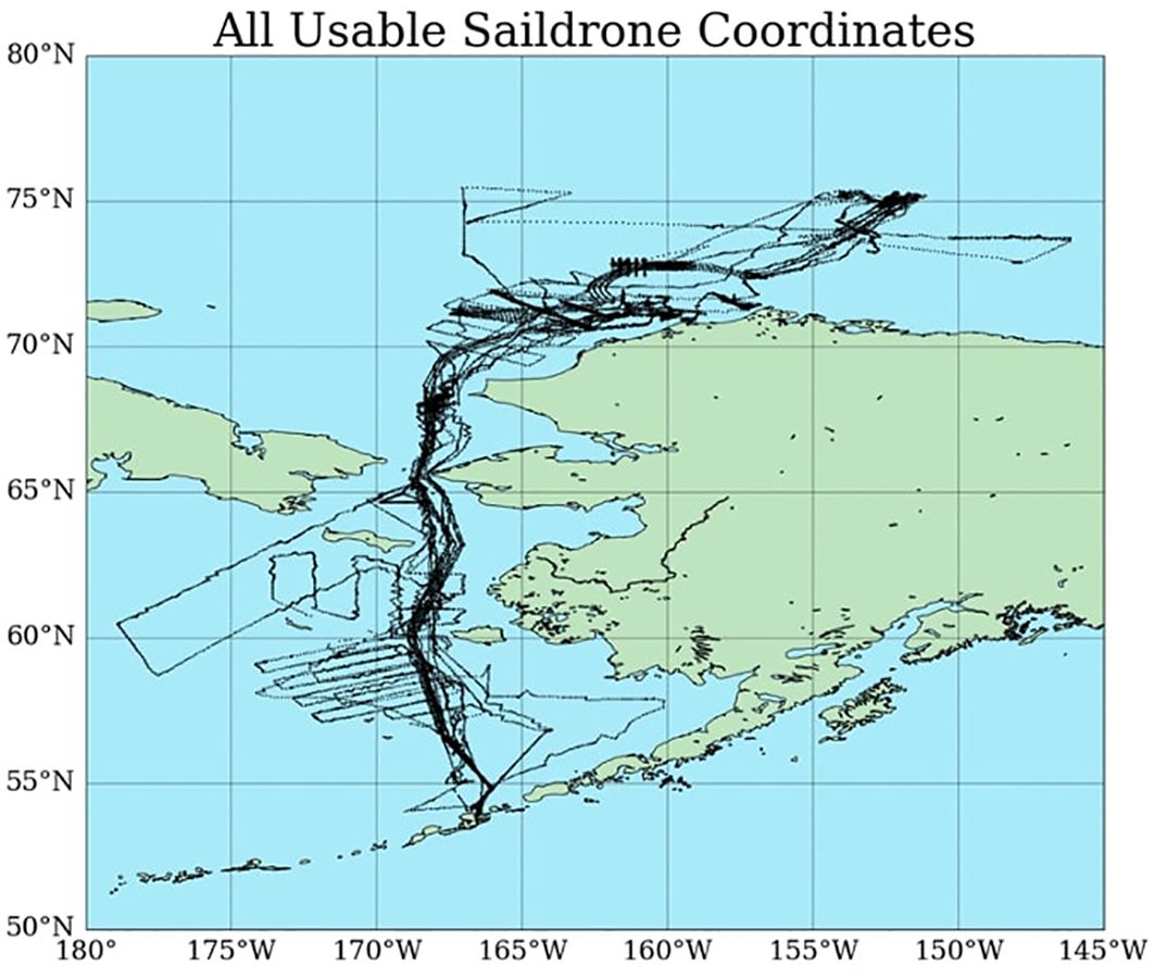
Figure 1 Locations of saildrone observations along their deployment tracks in the 2017, 2018, and 2019 missions.
Previous studies, such as those by Zhang et al. (2019) and Zhang et al. (2022), have extensively covered sensor configurations and data accuracy of saildrones; these details are not reiterated here. However, it is important to note that the temperature and humidity sensors on saildrones are mounted near the tips of horizontal booms, designed to always point into the wind from the sails. Additionally, the anemometers are mounted at the top of the sails. These placements ensure that the sensors are in optimal positions for taking measurements suitable for surface flux estimates.
2.2 Reanalysis products
This study evaluates three global reanalysis products: the NASA Global Modeling and Assimilation Office Modern-Era Retrospective Analysis for Research and Applications Version 2 (MERRA2, Gelaro et al., 2017), the European Centre for Medium-Range Weather Forecasts Atmospheric Reanalysis Version 5 (ERA5, Hersbach et al., 2020), and Climate Forecast System Reanalysis Version 2 (CFSR2, Saha et al., 2010). These reanalysis products include hourly surface flux data along with the surface state variables needed to estimate the fluxes. Their grid spacings are 0.625° x 0.25° for MERRA2, 0.25° x 0.25° for ERA5, and 0.5 x 0.5° for CFSR2. SST and 2-m temperature data for September 2018 are unavailable in CFSR2.
2.3 Pairing observations and reanalysis product data
Gridded hourly variables from the reanalysis products need to be paired with saildrone observations along their respective tracks for direct comparisons. This can be achieved through several methods. One involves interpolating gridded data to saildrones’ locations at a given hour. Because saildrone tracks are irregular relative to model grids, the four nearest grid points to a saildrone location at a given hour (e.g., the four corners of a grid box embedding a saildrone track during that hour) can be interpolated onto the saildrone’s location. Two issues need to be considered here: the temporal representation of gridded data at a given time and the spatial representation of a given grid. A model grid value for a state variable (e.g., temperature) at a given time, for instance, 0600 UTZ, normally represents the value precisely at that time. However, it would be inappropriate to compare the model grid value directly with a saildrone 1-min observation at 0600 UTC because the saildrone 1-min observation is precisely for that minute at that particular location, while the model grid value represents an average over a grid box. If ergodicity applies here, a spatially interpolated grid value onto a saildrone location at 0060 UTC should be compared with saildrone observations averaged over a time window centered at that time (e.g., 5:30 - 6:30 UTC) or equivalently, over a segment of the saildrone track centered at the location. This naturally leads to the second issue. If a model variable at a given grid represents an average over the grid box centered at that grid, there is no need to use data from other model grids. Saildrone observations should be compared to the reanalysis value at the nearest grid (the nearest neighbor method). Again, because of ergodicity, an average of saildrone data over time or along the track is still needed.
Temporal attributes of surface latent and sensible heat fluxes are more complicated. In some numerical model outputs, these fluxes are instantaneous values calculated using instantaneous state variables at a given time. In other numerical model outputs, these fluxes represent accumulated quantities over the model output interval. For instance, a flux value at 0600 UTC might represent the total flux accumulated from 0500 to 0600 UTC. In this case, fluxes based on saildrone observations should be integrated from 0500 to 0600 UTC.
In this study, we explored various methods for pairing gridded data from the reanalysis products with saildrone observations. These methods include spatial interpolations using inverse distance weighting (Shepard, 1968), bilinear interpolation, natural neighbor, and nearest neighbor methods (Li and Heap, 2008). We tested these methods with and without incorporating time averaging of saildrone data. These methods yield almost the same results, except for those that did not incorporate time averaging. Three factors may contribute to this insensitivity to the methods used. First, there is no complication from changing elevations, which would introduce sensitivities (Ahrens, 2006). Second, within an hour, a saildrone vehicle in most cases remained within the same reanalysis grid box (Figure 2) because of its slow motion, usually less than 9 km hr -1. Lastly, time averaging is not only physically logical in terms of ergodicity but also helps to filter out high-frequency fluctuations that are not resolved in the reanalysis products.
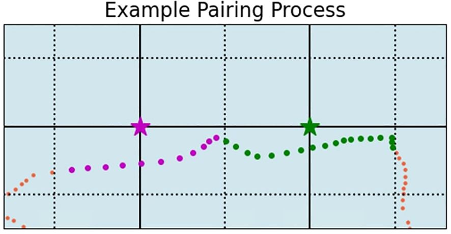
Figure 2 Illustration of the nearest neighbor method for pairing gridded reanalysis data with saildrone observations. Solid lines are grid lines of a reanalysis product. Dashed lines mark the grid boxes represented by the values at the grid points (stars). Reanalysis gridded values at the stars are paired with hourly mean saildrone observations at locations represented by the dots.
The results presented in the rest of this study are based on the nearest neighbor method, which is illustrated in Figure 2. At a given hour, the reanalysis data at specific grid points (marked as stars in Figure 2) are paired with observations from a saildrone. This pairing is based on the saildrone’s hourly averaged location (indicated by dots), centered on that hour, and positioned within the grid boxes (the dotted lines in Figure 2) represented by the grid points (the intersections of solid lines). When there is more than one saildrone in the same grid box at the same time, data from each saildrone is paired with the same gridded data and they are treated as independent samples in the reanalysis-saildrone comparison.
This method of pairing gridded reanalysis data with saildrone observations yields reasonable results. An example is given in Figure 3, which shows sensible fluxes from a saildrone (black dots) and their paired sensible fluxes from MERRA2 (blue), ERA5 (orange), and CFSR2 (green) in 2019. All these fluxes follow a similar pattern of fluctuations along the saildrone track during its deployment. From time to time, however, large discrepancies between them occur. A detailed and quantitative comparison of their fluxes is presented in section 3.
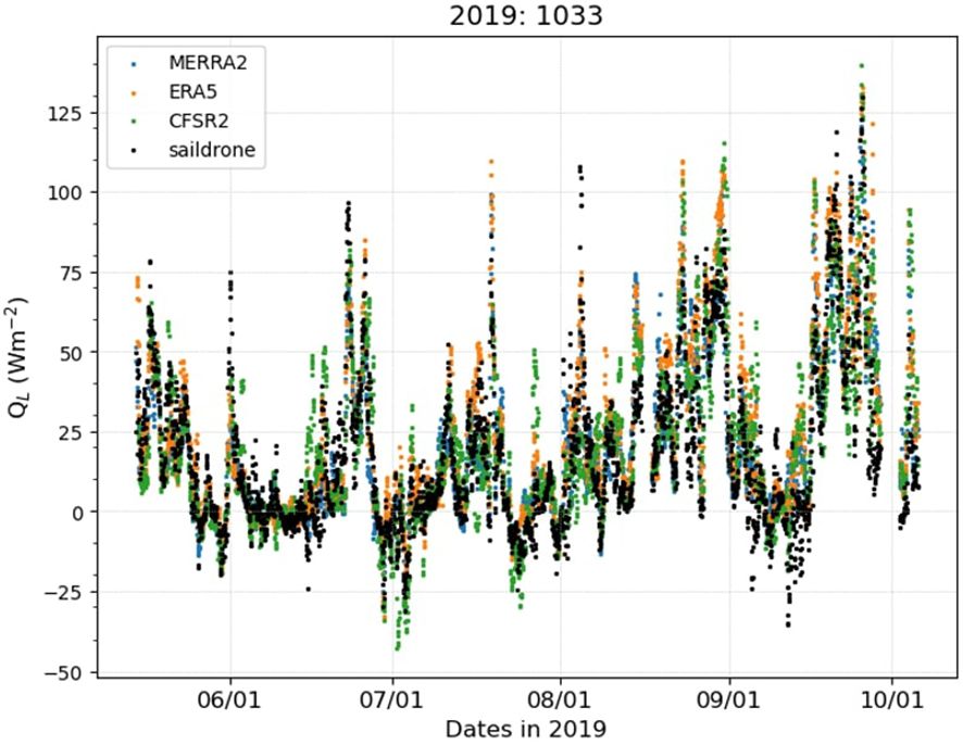
Figure 3 An example of paired sensible heat fluxes along the track of a saildrone (saildrone ID 1033) deployed in 2019. Black dots are for the saildrone, blue for MERRA2, orange for ERA5, and green for CFSR2.
When a saildrone track is close to a coastline, the nearest grid point of a reanalysis product can be over land, which must be excluded from the pairing. Removing such land points is necessary only for CFSR2 because of its coarser spatial grid distance. The total paired data for CFSR2 are therefore slightly less than the other two reanalysis products. Table 1 lists the numbers of paired data for each year and all three years combined. As a saildrone moves along its track, its location depends on the time. In consequence, all these reanalysis-saildrone paired data can be treated as sole functions of time.
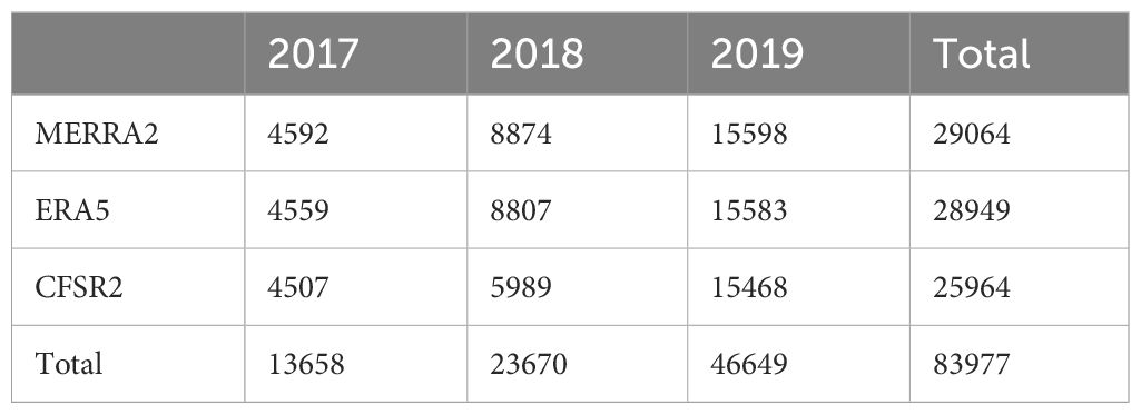
Table 1 Number of reanalysis-saildrone paired data points.
The discrepancies between the fluxes from the reanalysis products (Qre) and saildrone observations (Qobs) are defined as δQ = Qre - Qobs. We use the standard deviations (σ) of the surface fluxes observed by saildrones to measure whether the discrepancies are random or not. Discrepancies within ±σ are considered random, while those exceeding ±2σ large. The observed standard deviations (25 Wm-2 for latent heat fluxes and 19 Wm-2 for sensible heat fluxes) are calculated using all saildrone observations, encompassing both temporal and spatial variability. This results in higher values compared to standard deviations calculated at fixed locations over time. Therefore, this method is a very lenient measure for assessing random discrepancies and a stringent one for identifying large discrepancies.
3 Results
3.1 Comparison of fluxes
Interesting features can be revealed from visual inspections of the flux time series. As an example, Figure 4 shows the 2019 flux data from all six saildrone vehicles and their paired fluxes from the three reanalysis products. Each dot in the figure represents a specific time and its corresponding location along the saildrone tracks. The range of latent heat fluxes is larger than that of sensible heat fluxes in both the observations and reanalysis products, as previously observed in other parts of the Arctic open ocean (Fortuniak et al., 2017). There are much fewer negative values in latent heat fluxes (energy input into the ocean from the atmosphere) than positive values. This is evident in their probability distribution function (PDF, Figure 5) that includes all observed fluxes data from the three years. The PDF of the latent heat flux is heavily skewed toward the positive values, deviating substantially from the Gaussian distribution. In contrast, the PDF of the sensible heat flux is more symmetric around zero (although still positively skewed) and is closer to the Gaussian distribution than the latent heat fluxes. The positively skewed PDF of latent heat flux, which can be described in terms of a modified Fisher-Tippett distribution, is typical over the world’s oceans, while the semi-symmetric PDF of sensible heat flux is atypical, even in the boundary current upwelling regions (Gulev and Belyaev, 2012). This signifies the distinctive features of air-sea energy exchange in the Arctic environment.
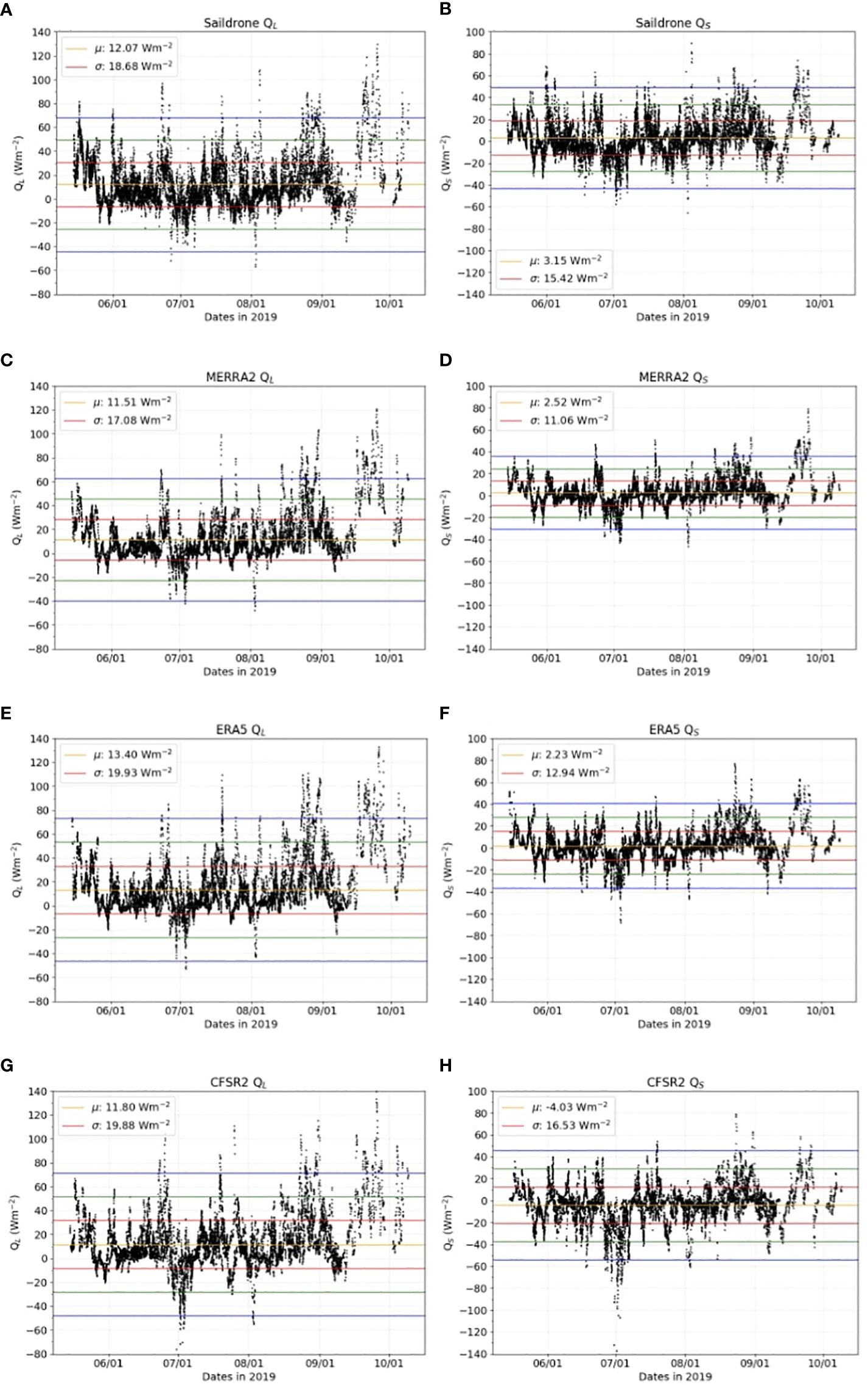
Figure 4 Latent heat fluxes (QL, left column) and sensible heat fluxes (QS, right) from saildrone observations (A, B), MERRA2 (C, D), ERA5 (E, F), and CFSR2 (G, H) in 2019 plotted as functions of time (month/day). Horizontal colored lines mark the time means (orange), ± 1 standard deviation (red), ± 2 standard deviations (green), and ±3 standard deviations (blue) for each flux dataset.
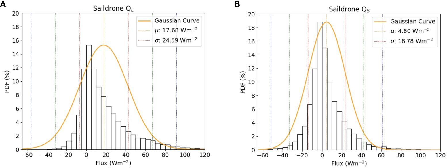
Figure 5 PDF of (A) QL and (B) QS from the saildrone observations of the three years. Solid curves are their Gaussian fits. Vertical lines mark the means (orange), and ±1 (red), ± 2 (green), and ±3 (blue) standard deviations.
Both Figures 3 and 4 suggest synoptic variations in time. Connecting these variations with Arctic weather systems requires information on large-scale perturbations, which we leave for future studies. As indicated by Figure 1, all missions started from Dutch Harbor, AK. In 2019 (Figure 3), the time of crossing the Bering Strait on their way to the north (outbound) was early June, and the time crossing the Bering Strait on their return to the south was mid-September. Figure 4 does not show evident differences between the Bering Sea (the beginning and end of the mission) and the Chukchi and Beaufort Seas (the middle of the mission).
The different PDFs for latent and sensible heat fluxes suggest that, in the Pacific Arctic region during May – October, warm air over a cold ocean surface (resulting in negative sensible heat fluxes) occurs more frequently than highly moist surface air that causes condensation at the ocean surface (resulting in negative latent heat fluxes). These negative sensible heat fluxes are of similar magnitude to those previously observed over the Arctic open ocean (Thorpe et al., 1973; Ganeshan and Wu, 2016; Thomson et al., 2018). Possible scenarios for higher surface air temperature than SST in the Arctic include intrusion of midlatitude synoptic systems (Liu and Barnes, 2015) and the influence of the warm sector of a cold front (Persson et al., 2005). Another possible factor is the continuous daylight in the Arctic region during the summer months, which leads to increased solar insolation and consequent warming of the surface air over land that could be advected over the ocean.
Quantitative comparisons of the latent and sensible fluxes from the reanalysis products and saildrone observations in terms of their means (μ) and standard deviations (σ) are given in Table 2. The time means of latent and sensible heat fluxes combined over the three years of saildrone measurement are positive, indicating that the ocean serves as a source of energy for the atmosphere in general during the summer. The standard deviations are larger than the means in both observations and reanalysis products. Fluxes generally fluctuate randomly (within ±σ) but are punctuated by sporadic, very large (> | ± 2σ|) spikes (Figure 4). The overall means and standard deviations in the reanalysis products are close to those in the observations. The differences in their means are smaller than the means themselves by an order of magnitude, and the differences in their standard deviations are also smaller than the standard deviations themselves by an order of magnitude. The only exception is the mean of sensible fluxes in CFSR2, which is of the opposite sign and differs from the observed mean by an amount larger than the mean itself. This indicates a non-negligible systematic and negative bias in sensible fluxes of CFSR2.
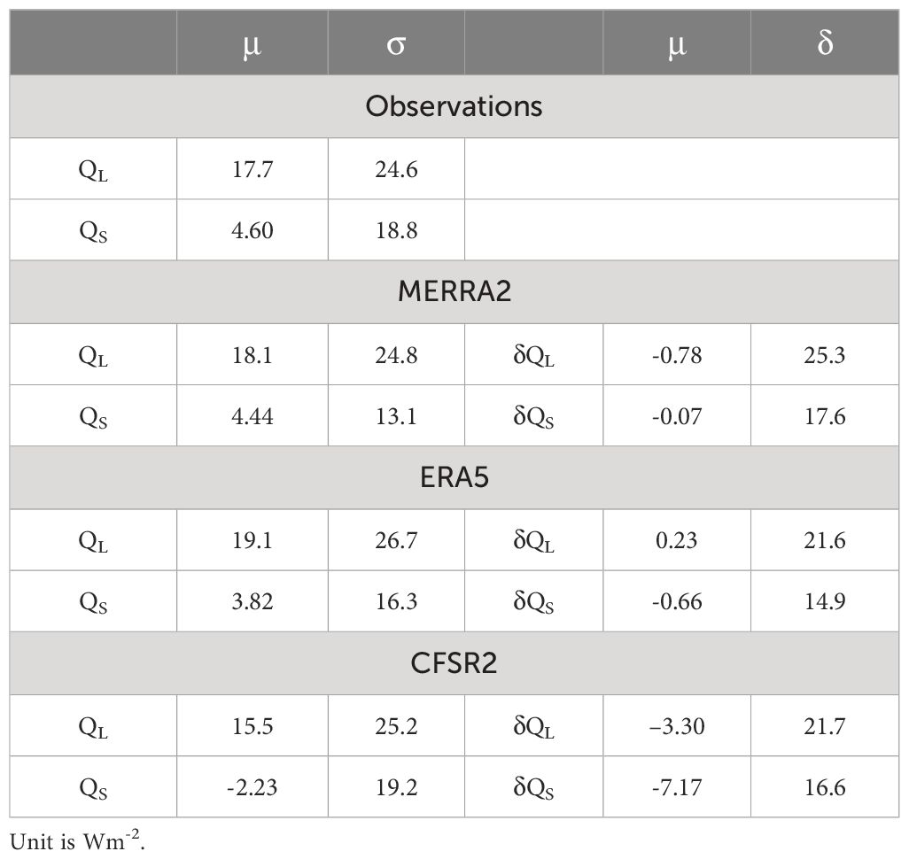
Table 2 Means (μ) and standard deviations (σ) of QL and QS in the observations and reanalysis products, and discrepancies (δQL and δQS) between the reanalysis products and observations for all three years.
Discrepancies in the surface fluxes between reanalysis products and observations (δQL and δQS) are generally within the observed one standard deviation (indicated by red horizontal lines in Figure 6). However, there are sporadic, large (> | ± 2σ|) spikes in δQL and δQS. The amplitudes of δQL and δQS are not related to the distances between the reanalysis grids and saildrone locations, which are 0 - 33 km for MERRA2/CFSR2 and 0–15.5 km for ERA5. Figure 6 seems to suggest that large spikes of δQL and δQS tend to occur between early June and mid-September when most saildrones are north of the Bering Strait. However, there is no evident dependence of δQL and δQS on the latitude of the saildrone locations when all three years of data are included.
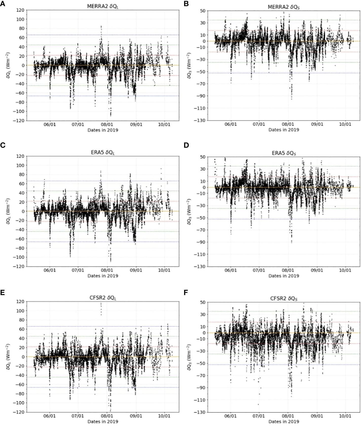
Figure 6 Discrepancies in latent heat fluxes (δQL, left column) and sensible heat fluxes (δQS, right) between observations and MERRA2 (A, B), ERA5 (C, D), and CFSR2 (E, F) in 2019 plotted as functions of time. Horizontal colored lines mark zeros (orange), ± 1 standard deviation (red), ± 2 standard deviations (green), and ±3 standard deviations (blue) of saildrone observations over the three years.
We can further compare how δQL and δQS distribute against the observed standard deviations σ (Table 3). More than 82% of δQL and δQS from MERRA2 and ERA5 are within | ± 1σ| of the saildrone observations, and less than 5% are more than | ± 2σ|. CFSR2 exhibits the largest δQS: it has the lowest percentage (75%) of data within the observed | ± 1σ| and the highest percentage (5.7%) of data exceeding | ± 2σ|. For MERRA2 and ERA5, δQL and δQS exceeding the observed | ± 1σ| are roughly evenly distributed between positive and negative values. In contrast, the number of large, negative δQS from CFSR2 is more than double that of its positive counterparts, contributing to the systematic negative biases in sensible heat fluxes of CFSR2. The negative bias in CFSR2 sensible heat fluxes also appears in the PDF of its δQS, which shows a Gaussian-like distribution as those of MERRA2 and ERA5 but shifts toward the negative side (not shown). Overall, large (>| ± 2σ|) δQL and δQS are infrequent but should not be ignored. They may reveal where reanalysis procedures need improvement.
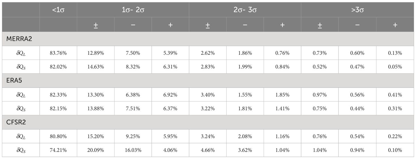
Table 3 Distribution of δQL and δQS in terms of observed standard deviations (σ).
Interestingly, the time series of δQL and δQS from the three reanalysis products have aligned fluctuation patterns, with some of their extremely large spikes occurring at similar times. These aligned spikes raise the question as to whether there are errors in the observations. One factor to consider is that, in several instances in 2019, saildrones were surrounded by sea ice (Chiodi et al., 2021). In these cases, calculating surface fluxes using open water algorithms and SST may have introduced large errors. However, large spikes of flux discrepancies also occurred in 2017 and 2018, when there was no sea ice near the saildrones. Therefore, sea ice cannot be the sole cause for all the large spikes in the discrepancies in Figure 6.
The fluxes from the observations and their paired fluxes from the reanalysis products are positively correlated in general (Figure 7). However, some extremely large values (>|± 3σ|) from the reanalysis products can occur when the observed fluxes are very small. Conversely, there are times when they are very small while the observed fluxes are very large. Their discrepancies (spread from the diagonal lines) tend to be larger when observed fluxes are large and positive than when the observed fluxes are large but negative. Renfrew et al. (2002) found systematic overestimates of both latent and sensible heat fluxes by ECMWF operational analyses and NCEP–NCAR reanalyses when fluxes are large (their Figure 6) over the Labrador Sea in February and March 1997. Their results are very different from what is shown in Figure 7, where both over- and under-estimates by ERA5 and CSFR2 are evident. It is unclear if the disagreement between the two studies comes from different times and locations, different versions of the reanalysis products, or both.
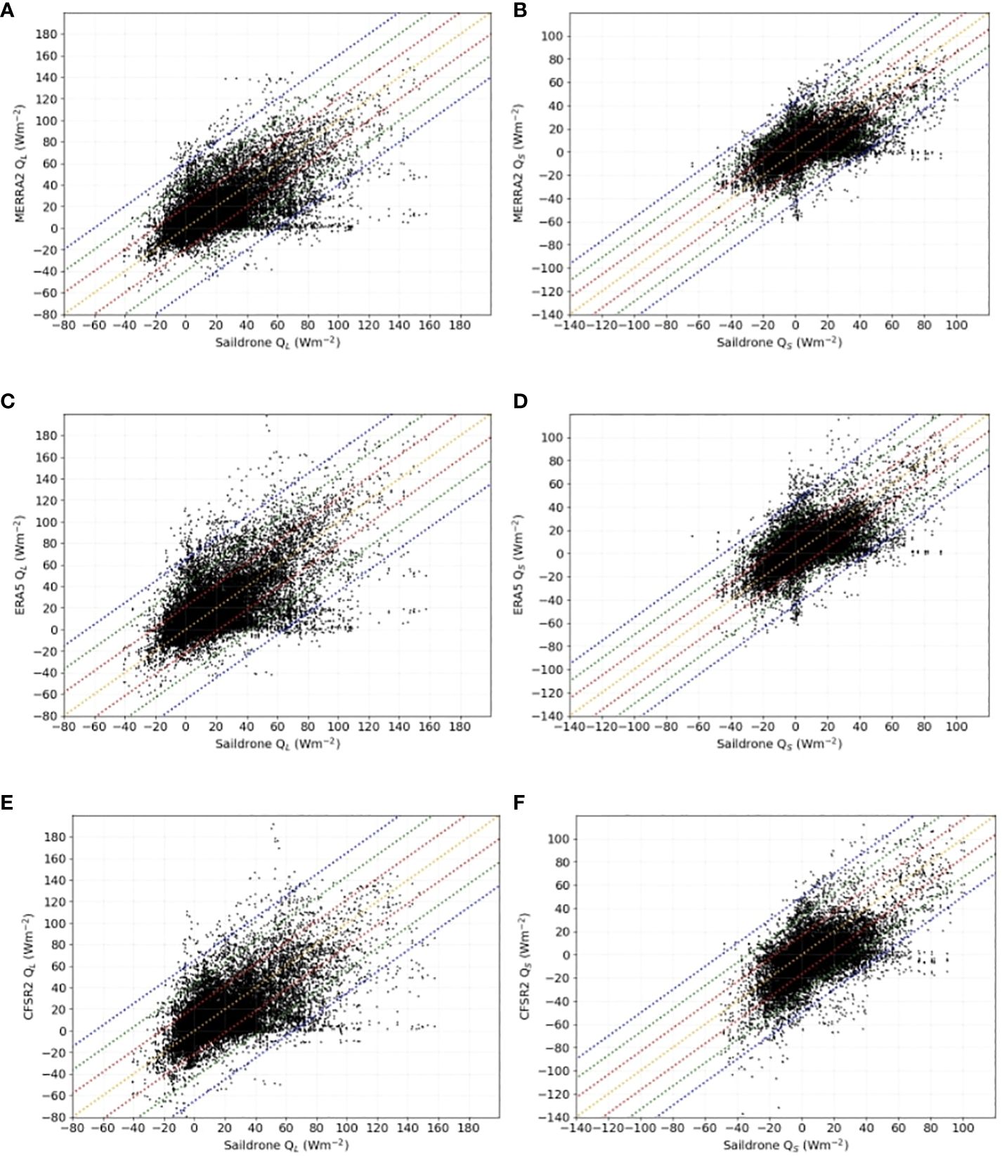
Figure 7 Scatter diagrams of QL and QS from the saildrone observations vs. MERRA2 (A, B), ERA5 (C, D), and CFSR2 (E, F) over the three years. Straight-colored lines mark the diagonal (orange), ± 1 standard deviation (red), ± 2 standard deviations (green), and ±3 standard deviations (blue) of saildrone observations.
3.2 Potential causes of large discrepancies
To explore the factors that may contribute to the very large discrepancies in the fluxes between the reanalysis products and observations (δQL and δQS), we use the simplest bulk formula (Yu, 2019) to guide our study, knowing that the fluxes in both the observations and reanalysis products were estimated using more sophisticated methods. The bulk formula for latent heat fluxes is:
where ρ is the density of surface air, LE the latent heat of evaporation, CE the exchange coefficient for latent heat, V the surface wind speed, and Δq = qs - qa the difference between surface saturation humidity qs and surface air humidity qa. Based on this bulk formula, if discrepancies between two latent heat flux datasets δQL are viewed as perturbations in the flux due to variations in each component in Equation (1), then δQL could stem from three main sources: discrepancies in their wind speed δV, the air-sea humidity difference δΔq, and the algorithms used δ(LECE). δQL can be broadly expressed as:
Differences in the algorithms, δ(ρLECE), may include treatments of LE and CE (whether constant or wind/temperature dependent), and parameterization of unresolved physical processes. These processes may include wind gusts, cooling by precipitation, convective cold pools, and thin ocean surface cold/warm layers, and fresh lenses, among others.
Similarly, the bulk formula for sensible heat fluxes is:
where CP is the specific heat capacity of air at a constant pressure, CH is the exchange coefficient for sensible heat, and ΔT = SST - Ta is the difference between SST and surface air temperature Ta. Discrepancies in sensible heat fluxes between two datasets, δQS, may arise from discrepancies in their wind speed δV, the air-sea temperature difference δΔT, and the algorithms used δ(CpCH). δQS in Equation (3) can be written as:
To assess the contributions of δV, δΔq, and δΔT to δQL and δQS, we first examine their amplitudes when δQL and δQS are large (> | ± 2σ|). Figures 8B, D, F show that for all three reanalysis products, large δQS critically depends on large δΔT (few large δQS occur when δΔT is near zero), whereas large δQS can occur at any value of δV, even at zero. However, the contribution of δΔT to δQS is not linear; the same δΔT can correspond to a wide range of δQS. This complexity may result from the flux algorithms, where exchange coefficients are not constant but depend on the thermodynamic conditions near the surface. For large δQL, δV and δΔq appear to contribute equally (Figures 8A, C, E). While large δQL can still occur at zero δV or zero δΔq, most of them occur when both δV or δΔq are large. These results are supported by the correlation between δQL, δQS and δV, δΔq, and δΔT (Table 4). For all three reanalysis products, the correlation coefficients between δQL and δΔq, R(δQL, δΔq), are slightly higher than R(δQL, δV), while their R(δQS, δΔT) are substantially higher than R(δQS, δV).
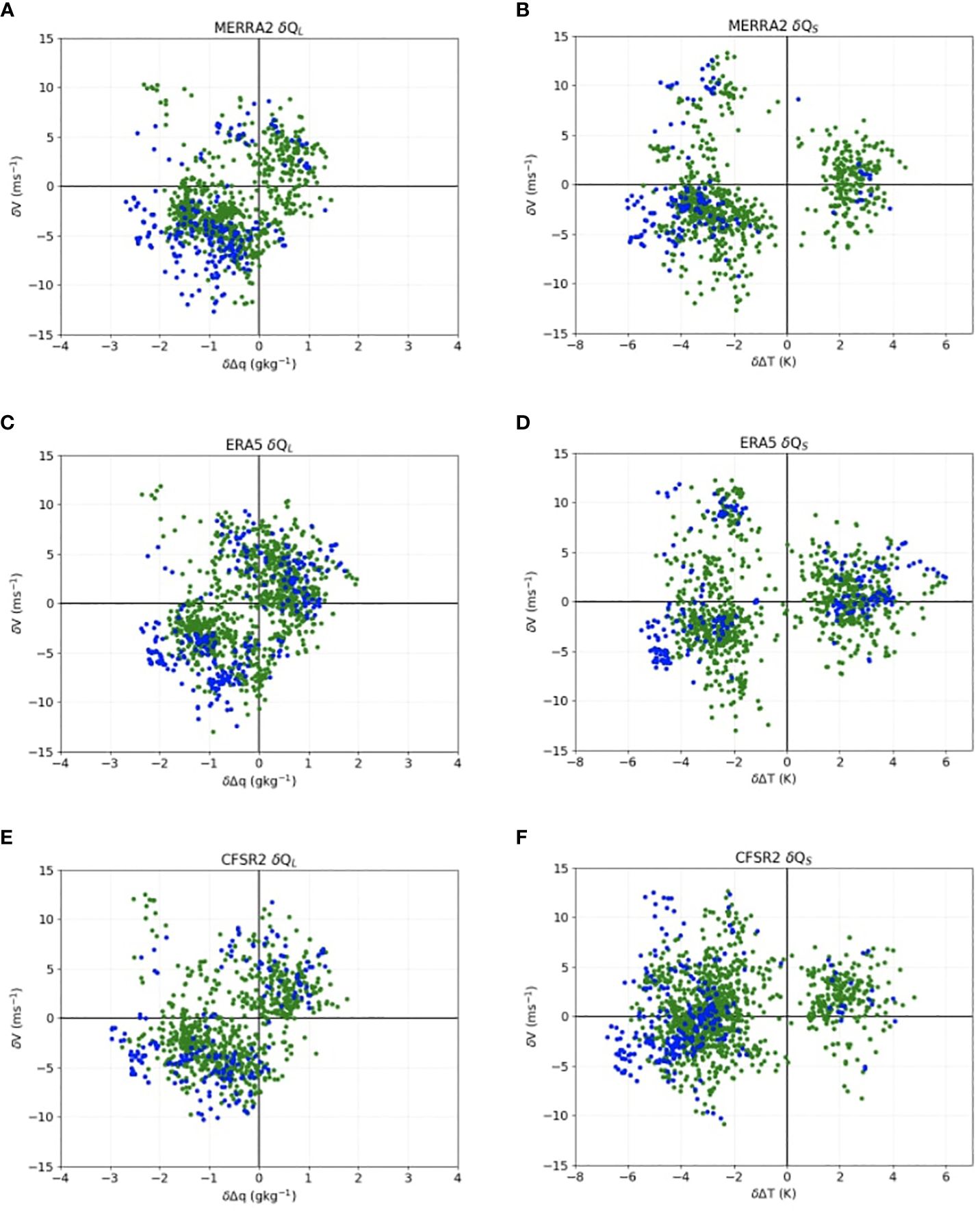
Figure 8 Scatter diagrams of δV vs. δΔq for large δQL (A, C, E) and δV vs. δΔT and large δQS (B, D, F) for the three reanalysis products. Colors represent |δQL| and |δQS| within observed 2 - 3 standard deviations (green) and greater than 3 standard deviations (blue).
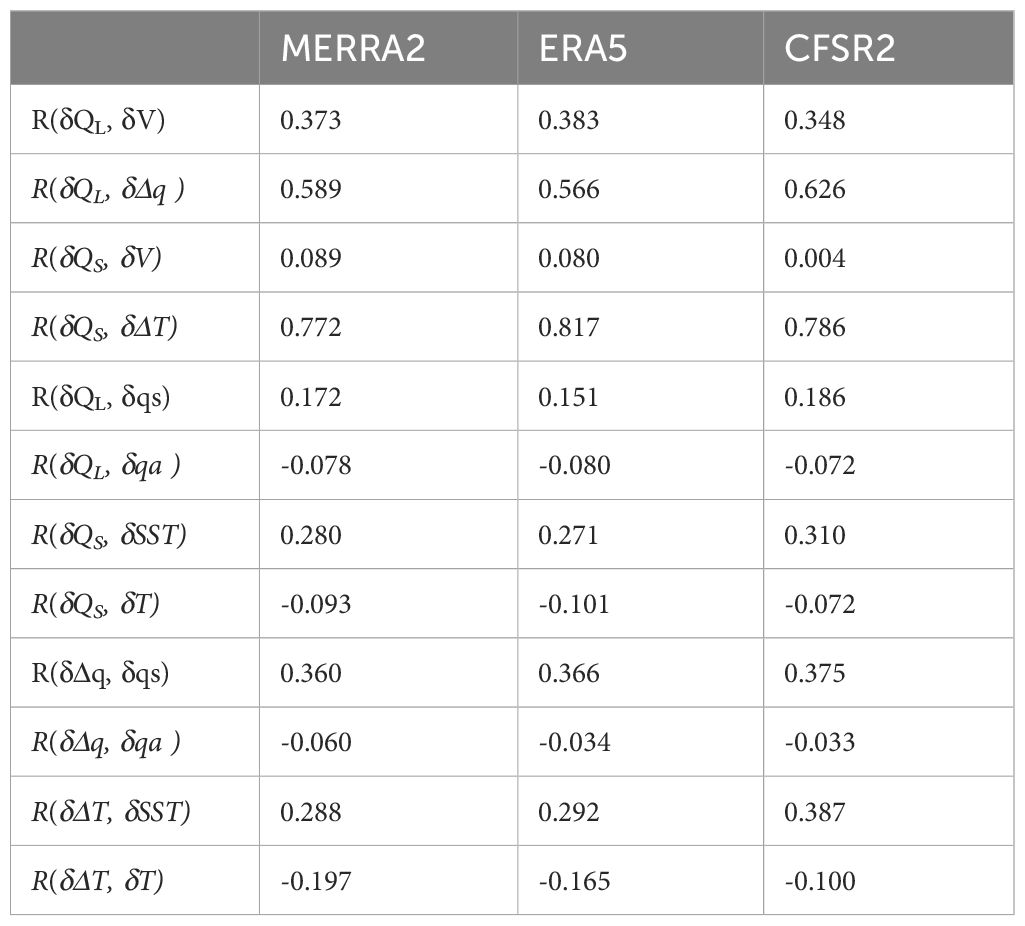
Table 4 Correlation coefficients (R) of reanalysis - saildrone discrepancies in latent and sensible heat fluxes (δQL, δQS) and those in wind speed (δV), air-sea differences in humidity (δΔq) and temperature (δΔT).
The impact of differences in the flux algorithms used (the second term on the right-hand sides of Equations 2, 4) on δQL and δQS can be estimated by applying the relevant state variables from the reanalysis products to the COARE algorithm used for calculating the saildrone fluxes. However, a more accurate approach would involve using surface state variables from saildrone observations (considered the “truth”) to the flux algorithms used to produce the reanalysis fluxes. Unfortunately, the algorithms for estimating reanalysis fluxes are not currently available to us. This possible exploration will be addressed in the future.
4 Discussion
This study is, to the best of our knowledge, the first that validates sea surface latent and sensible heat fluxes from global reanalysis products using observations from uncrewed surface vehicles in the Arctic. We used saildrone data to estimate these fluxes in the Pacific sector of the Arctic open ocean (the Bering, Chukchi, and Beaufort Seas) during the summers of 2017 – 2019. These observation-based flux estimates were compared with surface fluxes from three global reanalysis products: MERRA2, ERA5, and CFSR2. The results are mixed: encouraging in some respects and concerning in others. The mean differences between the reanalysis products and saildrone observations are negligibly small (< 1 Wm-2) in both latent and sensible heat fluxes for MERRA2 and ERA5, indicating no systematic biases. In contrast, the mean difference is more evident (< -3 Wm-2 in latent heat flux and< -7 Wm-2 in sensible heat flux) for CFSR2. In addition, the mean sensible heat fluxes from CFSR2 are negative while the observed is positive. These results indicate a systematic underestimation in the amplitude and a bias in the sign of surface sensible fluxes from CFSR2. Most discrepancies between the hourly data from the reanalysis products and saildrone observations, over 80% for MERRA2 and ERA5 but slightly lower (74 – 80%) for CFSR2, fall within the observed one standard deviation.
Surface fluxes in all three reanalysis products exhibit sporadic large discrepancies from the observed values, exceeding the observed two standard deviations (>| ± 2σ|), which is roughly equivalent to > | ± 50| Wm-2 for latent heat fluxes and > | ± 38| Wm-2 for sensible heat fluxes. These large discrepancies are mostly related to errors in the surface humidity and temperature within the reanalysis products. Additionally, errors in wind speeds in the reanalysis products have a greater impact on the discrepancies in latent heat fluxes than in sensible heat fluxes. Improvement of Arctic sea surface fluxes in the reanalysis products critically depends on their more accurate surface state variables, especially temperature, humidity, and wind.
The results from this study suggest that sea surface latent and sensible heat fluxes from MERRA2 and ERA5 can be treated as reliable proxies of observations to represent the mean state of air-sea fluxes in the Pacific sub-Arctic region. However, this assessment does not apply to CFSR2 due to its significant biases. The sporadic large discrepancies from the observations in all three reanalysis products lead to the conclusion that they may not be reliable for studies of air-sea energy exchange on short (e.g., synoptic) timescales in the Arctic. The results from this study provide guiding information to assess the applicability of surface latent and sensible heat fluxes in the three reanalysis products to high latitudes, which depend on the time and spatial scales of the processes under study that require different accuracies (Bourassa et al., 2013).
The causes of the large discrepancies in the fluxes between the reanalysis products and saildrone observation need to be further quantified in more detail. In particular, the almost synchronized large discrepancies among the three reanalysis products (Figure 6) suggest potential common sources of errors. A possible source could be satellite observations, which are included in the production of all three analyses to different extents. Satellite retrievals of SST face many challenges including the presence of sea ice (Castro et al., 2023). Saildrone SST measured at a certain depth is not corrected to skin SST, while SST used in the reanalysis is skin SST. Under low-wind conditions (< 3 ms-1) difference between measured and skin SST can be larger than 0.3°C (Jia et al., 2023). But Figure 8 clearly shows that δQS does not exclusively depend on wind speed, ruling out measured vs. skin SST difference as a major source of δQS. This leaves surface humidity and air temperature as the most likely sources of the discrepancies. Zhang et al. (2022) found large errors in surface air temperature, humidity, and SST in the initial conditions of numerical weather forecasts in the Arctic from several global models. It would not be surprising if it is also the case for the reanalysis products, but this needs to be confirmed and quantified.
The validation approach used in this study can be applied to evaluate surface heat fluxes produced by numerical weather prediction models and climate models. This work is currently underway. It can also be applied to compare surface heat fluxes from saildrone observations and other global datasets that cover the period of saildrone deployments (since 2017), such as the Objectively Analyzed Air-Sea Fluxes (OAFlux), which are constructed using data from in situ observations, satellites and reanalysis products (Yu and Weller, 2007). Saildrone data are currently not included in OAFlux and can serve as independent data for validation. Air-sea heat fluxes are vital to the study of climate change, especially in sensitive areas such as the Arctic region. Some of these areas are very difficult to access for in situ observations except when using uncrewed observing systems. The dataset of air-sea fluxes in this study, based on saildrone observations, is perhaps the largest in situ air-sea flux dataset of the sub-Arctic open ocean by data points. But it is limited to three summers and specific regions of the Pacific sector of the sub-Arctic. Expanding the scope of in situ observations would be beneficial to investigate potential regional and seasonal variations in the accuracy of surface heat fluxes in the global reanalysis products. Arctic amplification is the strongest in winter months (Previdi et al., 2021). It would be desirable to observe sea surface fluxes in winter if the challenge of sea ice detection and avoidance can be met (Chiodi et al., 2021). It is also desirable to compare saildrone observations with those from other platforms (ships, moored buoys, drifters, airborne dropsondes, and ocean profilers) to assess their consistency. Up to date, deployments of those platforms have been extremely sparse for the Arctic open ocean and there have been no observations near saildrones for direct comparisons. In the future, coordinated Arctic in situ observations are needed to design and execute collocated observations from diverse platforms to cross-check and validate their accuracies.
Data availability statement
The original contributions presented in the study are included in the article. Further inquiries can be directed to the corresponding author. The saildrone observations are available from:
https://data.pmel.noaa.gov/generic/erddap/search/index.html?page=1&itemsPerPage=1000searchFor=saildrone. The reanalysis data were downloaded from:
https://www.soest.hawaii.edu/soestwp/research/org/centers/asia-pacific-data-research-center-apdrc/ https://cds.climate.copernicus.eu/cdsapp#!/dataset/reanalysis-era5-single-levels?tab=overview.
Author contributions
SS: Writing – original draft, Writing – review & editing. CZ: Writing – original draft, Writing – review & editing. DZ: Writing – review & editing. LY: Writing – review & editing. ID: Writing – review & editing.
Funding
The author(s) declare financial support was received for the research, authorship, and/or publication of this article. The funding for this study was provided by the NOAA William M. Lapenta Internship Program (SS), NOAA PMEL (CZ), the Cooperative Institute for Climate, Ocean, & Ecosystem Studies (CIOCES) under NOAA Cooperative Agreement NA20OAR4320271 (DZ), the NOAA Ocean Monitoring and Observing (GOMO) program, Grant NA19OAR4320074 (LY), and the NOAA Ernest F. Hollings Scholarship Program (ID).
Acknowledgments
SS would like to thank the NOAA William M. Lapenta Internship Program for the support to her visit to the Pacific Marine Environmental Laboratory (PMEL) in the summer of 2022, the faculty, staff, and students at the University of Maryland Atmospheric and Ocean Science for their constructive feedback to the study. SS would also like to thank Eli Lichtblau for their programming support. ID was supported by the NOAA Ernest F. Hollings Scholarship Program for her visit to PMEL in the summer of 2023. Comments from James Overland, Ola Person, Chris Fairall, and Elizabeth Thompson are appreciated. This is PMEL contribution #5581. This is CICOES Contribution No. 2024-1379.
Conflict of interest
The authors declare that the research was conducted in the absence of any commercial or financial relationships that could be construed as a potential conflict of interest.
Publisher’s note
All claims expressed in this article are solely those of the authors and do not necessarily represent those of their affiliated organizations, or those of the publisher, the editors and the reviewers. Any product that may be evaluated in this article, or claim that may be made by its manufacturer, is not guaranteed or endorsed by the publisher.
References
Ahrens B. (2006). Distance in spatial interpolation of daily rain gauge data. Hydrol. Earth Sys. Sci. 10, 197–208. doi: 10.5194/hess-10-197-2006
Andreas E. L. (1987). A theory for the scalar roughness and the scalar transfer coefficients over snow and sea ice. Boundary-Layer Meteorol. 38, 159–184. doi: 10.1007/BF00121562
Batrak Y., Müller M. (2019). On the warm bias in atmospheric reanalyses induced by the missing snow over Arctic sea-ice. Nat. Commun. 10, 4170. doi: 10.1038/s41467-019-11975-3
Bentemy A., Piolle J. F., Grouazel A., Danielson R., Gulev S., Paul F., et al. (2017). Review and assessment of latent and sensible heat flux accuracy over the global oceans. Remote Sens. Environ. 201, 196–218. doi: 10.1016/j.rse.2017.08.016
Boisvert L. N., Wu D. L., Vihma T., Susskind J. (2015). Verification of air/surface humidity differences from AIRS and ERA-Interim in support of turbulent flux estimation in the Arctic. J. Geophys. Res.: Atmos. 120, 945–963. doi: 10.1002/2014JD021666
Bourassa M. A., Gille S.T., Bitz C., Carlson D., Cerovecki I., Clayson C.A.vv, et al. (2013). High-latitude ocean and sea ice surface fluxes: Challenges for climate research. Bull. Am. Meteorol Soc. 94, 403–423. doi: 10.1175/BAMS-D-11-00244.1
Bromwich D. H., Wilson A.B., Bai L., Liu Z., Barlage M., Shih C.F., et al. (2018). The Arctic system reanalysis, version 2. Bull. Am. Meteorol Soc. 99, 805–828. doi: 10.1175/BAMS-D-16-0215.1
Castro S. L., Wick G. A., Eastwood S., Steele M. A., Tonboe R.T.vv (2023). Examining the consistency of sea surface temperature and sea ice concentration in arctic satellite products. Remote Sensing. 15, 2908. doi: 10.3390/rs15112908
Chiodi A. M., Zhang C., Cokelet E. D., Yang Q., Mordy C. W., Gentemann C., et al. (2021). Exploring the Pacific arctic seasonal ice zone with saildrone USVs. Front. Mar. Sci. 8. doi: 10.3389/fmars.2021.640697
Decker M., Brunke M.A., Wang Z., Sakaguchi K., Zeng X., Bosilovich M.G. (2012). Evaluation of reanalysis products from GSFC, NCEP, and ECMWF using Flux Tower Observations. J. Climate. 25, 1916–1944. doi: 10.1175/JCLI-D-11-00004.1
Edson J. B., Hinton A.A., Prada K.E., Hare J.E., Fairall C.W. (1998). Direct covariance flux estimates from mobile platforms at sea. J. Atmos Ocean. Technol. 15, 547–562. doi: 10.1175/1520-0426(1998)015<0547:DCFEFM>2.0.CO;2
Edson J. B., et al. (2013). On the exchange of momentum over the Open Ocean. J. Phys. Oceanogr. 43, 1589–1610. doi: 10.1175/JPO-D-12-0173.1
Fairall C. W., et al. (2003). Bulk parameterization of air–sea fluxes: Updates and verification for the COARE algorithm. J. Climate. 16, 571–591. doi: 10.1175/1520-0442(2003)016<0571:BPOASF>2.0.CO;2
Fortuniak K., et al. (2017). Sea water surface energy balance in the Arctic fjord (Hornsund, SW Spitsbergen) in May–November 2014. Theor. Appl. Climatol. 128, 959–970. doi: 10.1007/s00704-016-1756-3
Ganeshan M., Wu D. L. (2016). The open-ocean sensible heat flux and its significance for Arctic boundary layer mixing during early fall. Atmos Chem. Phys. 16, 13173–13184. doi: 10.5194/acp-16-13173-2016
Gelaro R., McCarty W., Suárez M. J., Todling R., Molod A., Takacs L., et al. (2017). The modern-era retrospective analysis for research and applications, version 2 (MERRA-2). J. Climate. 30, 5419–5454. doi: 10.1175/JCLI-D-16-0758.1
Gentemann C. L., Clayson C. A., Brown S., Lee T., Parfitt R., Farrar J. T., et al. (2020). FluxSat: measuring the ocean–atmosphere turbulent exchange of heat and moisture from space. Remote Sensing. 12, 1796. doi: 10.3390/rs12111796
Graham R. M., Cohen L., Ritzhaupt N., Segger B., Graversen R.G., Rinke A., et al. (2019). Evaluation of six atmospheric reanalyses over Arctic sea ice from winter to early summer. J. Climate. 32, 4121–4143. doi: 10.1175/JCLI-D-18-0643.1
Graversen R. G., Mauritsen T., Drijfhout S., Tjernström M., Mårtensson S. (2011). Warm winds from the Pacific Cause extensive Arctic sea-ice melt in summer 2007. Climate dynam. 36, 2103–2112. doi: 10.1007/s00382-010-0809-z
Gulev S. K., Belyaev K. (2012). Probability distribution characteristics for surface air-sea turbulent heat fluxes over the global ocean. J. Climate. 25, 184–206. doi: 10.1175/2011JCLI4211.1
Hersbach H., Bell B., Berrisford P., Dahlgren P., Horányi A., Munoz-Sebater J., et al. (2020). The ERA5 global reanalysis. Q. J. R. Meteorol Soc. 146, 1999–2049. doi: 10.5194/egusphere-egu2020-10375
Intrieri J. M., et al. (2002). An annual cycle of Arctic Surface Cloud Forcing at SHEBA. J. Geophys. Res.: Oceans. 107, SHE-13. doi: 10.1029/2000JC000439
Jackson D. L., Wick G. A. (2010). Near-surface air temperature retrieval derived from AMSU-A and sea surface temperature observations. J. Atmos Ocean. Technol. 27, 1769–1776. doi: 10.1175/2010JTECHA1414.1
Jakobsen E., Vihma T., Palo T., Jakobson L., Keernik H., Jaagus J. (2012). Validation of atmospheric reanalyses over the central Arctic Ocean. Geophys. Res. Letters. 39. doi: 10.1029/2012GL051591
Jia C., Minnett P.J., Luo B. (2023). Significant diurnal warming events observed by saildrone at high latitudes. J. Geophys. Res.: Oceans 128. doi: 10.1029/2022JC019368
Justino F., Wilson A.B., Bromwich D.H., Avila A., Bai L.S., Wang S.H. (2019). Northern Hemisphere extratropical turbulent heat fluxes in ASRv2 and global reanalyses. J. Climate. 32, 2145–2166. doi: 10.1175/JCLI-D-18-0535.1
Kim K. Y., Hamlington B.D., Na H., Kim J. (2016). Mechanism of seasonal Arctic sea ice evolution and Arctic amplification. Cryosphere. 10, 2191–2202. doi: 10.5194/tc-10-2191-2016
Li J., Heap A. D. (2008). A review of spatial interpolation methods for environmental scientists. Geosci. Australia. 23, 137–145.
Liu C., Barnes E. A. (2015). Extreme moisture transport into the Arctic linked to Rossby wave breaking. J. Geophys. Res.: Atmos. 120, 3774–3788. doi: 10.1002/2014JD022796
Lüpkes C., Vihma T., Jakobson E., König‐Langlo G., Tetzlaff A. (2010). Meteorological observations from ship cruises during summer to the central Arctic: a comparison with reanalysis data. Geophys. Res. Letters. 37. doi: 10.1029/2010GL042724
Meinig C., Burger E.F., Cohen N., Cokelet E.D., Cronin M.F., Cross J.N., et al. (2019). Public-private partnerships to advance regional ocean-observing capabilities: A Saildrone and NOAA-PMEL case study and future considerations to expand to global scale observing. Front. Mar. Sci. 6. doi: 10.3389/fmars.2019.00448
Moore G. W. K., Renfrew I.A., Pickart R.S. (2012). Spatial distribution of air-sea heat fluxes over the sub-polar North Atlantic Ocean. Geophys. Res. Lett. 39. doi: 10.1029/2012GL053097
Persson G., Hare P.O., Fairall J.E., Otto C.W., W.D. (2005). Air–sea interaction processes in warm and cold sectors of extratropical cyclonic storms observed during FASTEX. Q. J. R. Meteorol Soc. 131, 877–912. doi: 10.1256/qj.03.181
Previdi M., Smith K.L., Polvani L.M. (2021). Arctic amplification of climate change: a review of underlying mechanisms. Environ. Res. Letters. 16. doi: 10.1088/1748-9326/ac1c29
Rantanen M., Karpechko A.Y., Lipponen A., Nordling K., Hyvärinen O., Ruosteenoja K., et al. (2022). The Arctic has warmed nearly four times faster than the globe since 1979. Nat. Commun. 3, 168. doi: 10.1038/s43247-022-00498-3
Renfrew I. A., Moore G.K., Guest P.S., Bumke K. (2002). A comparison of surface layer and surface turbulent flux observations over the Labrador Sea with ECMWF analyses and NCEP reanalyses. J. Phys. Oceanogr. 32, 383–400. doi: 10.1175/1520-0485(2002)032<0383:ACOSLA>2.0.CO;2
Saha S., Moorthi S., Pan H.L., Wu X., Wang J., Nadiga S., et al. (2010). The NCEP climate forecast system reanalysis. Bull. Am. Meteorol Soc. 91, 1015–1058. doi: 10.1175/2010BAMS3001.1
Schlüssel P., et al. (1995). Retrieval of latent heat flux and longwave irradiance at the sea surface from SSM/I and AVHRR measurements. Adv. Space Res. 16, 107–116. doi: 10.1016/0273-1177(95)00389-V
Screen J. A., Simmonds I. (2010a). Increasing fall-winter energy loss from the Arctic Ocean and its role in Arctic temperature amplification. Geophys. Res. Letters. 37. doi: 10.1029/2010GL044136
Screen J. A., Simmonds I. (2010b). The central role of diminishing sea ice in recent Arctic temperature amplification. Nature 464, 1334–1337. doi: 10.1038/nature09051
Selivanova J. V., Tilinina N. D., Gulev S. K., Dobrolubov S. A.. (2016). Impact of ice cover in the Arctic on ocean–atmosphere turbulent heat fluxes. Oceanology 56, 14–18. doi: 10.1134/S0001437016010185
Serreze M. C., Francis J. A. (2006). The Arctic amplification debate. Clim. change. 76, 241–264. doi: 10.1007/s10584-005-9017-y
Shepard D. (1968). “A two-dimensional interpolation function for irregularly-spaced data,” in Proceedings of the 1968 23rd ACM national conference (New York, NY, United States: Association for Computing Machinery), Vol. 23. 517–524. doi: 10.1145/800186.810616
Stabeno P. J., Bond N.A., Salo S.A. (2007). On the recent warming of the southeastern Bering Sea Shelf. Deep-Sea Res. Part II. 54, 2599–2618. doi: 10.1016/j.dsr2.2007.08.023
Steele M., Zhang J., Ermold W. (2010). Mechanisms of summertime upper Arctic ocean warming and the effect on sea ice melt. J. Geophys. Res.: Oceans. 115. doi: 10.1029/2009JC005849
Taylor P. C., et al. (2018). On the increasing importance of air-sea exchanges in a thawing Arctic: A Review. Atmosphere 9, 41. doi: 10.3390/atmos902004
Thomson J., Ackley S., Girard‐Ardhuin F., Ardhuin F., Babanin A., Boutin G., et al. (2018). Overview of the arctic sea state and boundary layer physics program. J. Geophys. Res.: Oceans. 123, 8674–8687. doi: 10.1002/2018JC013766
Thorpe M. R., Banke E. G., Smith S. D. (1973). Eddy correlation measurements of evaporation and sensible heat flux over Arctic sea ice. J. Geophys. Res. 78, 3573–3584. doi: 10.1029/JC078i018p03573
Uttal T., Yang Q., Li X., Yuan X., Bushuk M., Chen D. (2002). Surface heat budget of the Arctic Ocean. Bull. Am. Meteorol Soc. 83, 255–276. doi: 10.1175/1520-0477(2002)083<0255:SHBOTA>2.3.CO;2
Yu L. (2019). Sea surface exchanges of momentum, heat, and freshwater determined by satellite remote sensing. Encyclo. Ocean Sci., 15–23. doi: 10.1016/B978-0-12-409548-9.11458-7
Yu L., Weller R. A. (2007). Objectively analyzed air–sea heat fluxes for the global ice-free oceans, (1981–2005). Bull. Am. Meteorol Soc. 88, 527–540. doi: 10.1175/BAMS-88-4-527
Zeng J., Yang Q., Li X., Yuan X., Bushuk M., Chen D., et al. (2023). Reducing the spring barrier in predicting summer Arctic sea ice concentration. Geophys. Res. Letters. 50. doi: 10.1029/2022GL102115
Zhang D., Chiodi A.M., Zhang C., Foltz G.R., Cronin M.F., Mordy C.W., et al. (2019). Comparing air-sea flux measurements from a new unmanned surface vehicle and proven platforms during the SPURS-2 field campaign. Oceanography 32, 122–133. doi: 10.5670/ocean
Zhang C., Levine A.F., Wang M., Gentemann C., Mordy C.W., Cokelet E.D., et al. (2022). Evaluation of surface conditions from operational forecasts using in situ saildrone observations in the Pacific arctic. Month. Weather Rev. 150, 1437–1455. doi: 10.1175/MWR-D-20-0379.1
Zhang C., et al. (2023). Hurricane observations by uncrewed systems. Bull. Am. Meteorol Soc. 104, E1893–E1917. doi: 10.1175/BAMS-D-21-0327.1
Keywords: Arctic, saildrone, global reanalysis product, latent heat flux, sensible heat flux
Citation: Sivam S, Zhang C, Zhang D, Yu L and Dressel I (2024) Surface latent and sensible heat fluxes over the Pacific Sub-Arctic Ocean from saildrone observations and three global reanalysis products. Front. Mar. Sci. 11:1431718. doi: 10.3389/fmars.2024.1431718
Received: 12 May 2024; Accepted: 18 June 2024;
Published: 12 July 2024.
Edited by:
Donald B. Olson, University of Miami, United StatesReviewed by:
Lei Zhou, Shanghai Jiao Tong University, ChinaHailun He, Ministry of Natural Resources, China
Copyright © 2024 Sivam, Zhang, Zhang, Yu and Dressel. This is an open-access article distributed under the terms of the Creative Commons Attribution License (CC BY). The use, distribution or reproduction in other forums is permitted, provided the original author(s) and the copyright owner(s) are credited and that the original publication in this journal is cited, in accordance with accepted academic practice. No use, distribution or reproduction is permitted which does not comply with these terms.
*Correspondence: Subhatra Sivam, c3ViaGF0cmEuc2l2YW1AZ21haWwuY29t">subhatra.sivam@gmail.com