Fine spatio-temporal prediction of fishing time using big data

Overfishing, bycatch, and other anthropogenic threats may lead to the destruction of fragile habitats and substantial losses of marine life. Marine fishery resources can be protected by adjusting fishing intensity and establishing marine reserves. Currently, China adopts the closed fishing season management approach to protect traditional fishing grounds, where fine spatio-temporal prediction is essential to efficiently supervise the wide scope. Fishing vessel behaviors reflect fishers’ experience as well as the information provided by fish detection radar, while the fishery resource distribution is relevant to the marine environment. In this study, we identified fishing vessel behaviors (gillnets, trawls, purse seines, and abnormal behaviors) and qualitatively assessed and predicted fishing time of different fishing vessel behaviors to search for high intensity fishing operation areas by constructing a time-space prediction model. The model was based on big data of fishing vessel automatic identification systems and3 the marine environment, and was verified in the East China Sea. The prediction results generally corresponded with the distribution of traditional fishery resources in the East China Sea and the fishing efforts provided by the Global Fishing Watch. This model can provide an accurate and effective refined fishing vessel operation time prediction, and benefits fishing management and fishery resources protection.

1 Introduction

The marine ecosystem plays a crucial role in maintaining the global ecological balance and is resource-rich. Many coastal countries have acknowledged the development and utilization of marine resources as the key development direction in the new century. However, human pressure on marine resources and demand for marine ecosystem services are often too high (EC Reg, 2008; Davies et al., 2022). Under the cumulative impact of various human activities, the marine ecosystem quickly degrades (Costello et al., 2010; Halpern et al., 2015). Fishing is a main factor that affects the marine ecosystem (Jackson et al., 2001). Globally, most fish stocks are caught at the maximum sustainable, or even unsustainable rates (Ortuño Crespo and Dunn, 2017). High intensity fishing efforts may lead to oceanic resource collapse, and also cause habitat structure degradation or loss (Turner et al., 1999). Therefore, efficient fishery supervision and marine fishery resource protection, along with the marine ecological environment, has become a top priority.

Traditional fishery management adopts a population-based approach, focusing on adjusting fishing effort of a single target species to the level of maximum sustainable yield (Crowder et al., 2008). In addition to protecting the target individual populations affected by fishing, marine reserves have been set up worldwide in recent decades to provide lasting protection for marine ecosystems (Gerber et al., 2002; Jones, 2002; Lubchenco et al., 2003; Cimino et al., 2019), but the wide range of marine reserves leads to low regulatory efficiency. Recently, the emergence of the Automatic Identification System (AIS) has provided accurate space-time and behavioral information about fishing vessels, creating conditions for effective fishery supervision. The potential role of the AIS in fishery management has been recognized by the International Council for the Exploration of the Sea (ICES) (Ferrà et al., 2018). In terms of assessing the fishing intensity of fishing vessels, Natale et al. (2015) determined the fishing grounds and fishing effort of trawlers based on AIS data, and verified the method using detailed log data. Ferrà et al. (2018) used AIS data to assess the range of bottom trawling activities in the Mediterranean Sea over three years. Furthermore, Rodríguez et al. (2021) used AIS data to measure fishing efforts in the high seas and found that fishing effort concentrates along narrow strips attached to the boundaries of EEZs with productive fisheries. The aforementioned studies offer a scientific foundation for fishery production and management, while also contributing to environmental conservation and the sustainable development of fishery resources. However, previous works mostly assessed historical fishing efforts, which lacked a certain degree of timeliness for fisheries regulation. The challenge lies in selecting high intensity fishing vessel operation areas for different types of vessels and dynamically adjusting patrol routes for the coming days based on temporal and marine environmental shifts to enhance the efficiency of fishery regulation remains an unresolved issue.

In this study, using the AIS and Beidou Vessel Monitoring System (VMS) big data of fishing vessels, we (i) modeled fishing vessel behavior to recognize gillnets, trawls, purse seines, and abnormal behaviors, and on this basis, conducted qualitative estimation of fishing time of different fishing vessel behaviors, (ii) established a coupling model of fishing time and marine environment big data, and (iii) applied marine environment forecast data and the coupled models to search for daily high intensity fishing operation areas of different fishing vessel behaviors in the coming days.

2 Data

2.1 Fishing vessel big data

Beidou VMS is a vessel monitoring system that utilizes China’s Beidou satellite positioning. It mainly consists of four parts: Beidou satellite navigation system, onshore monitoring center, shipborne terminal, and Beidou operation service center, and was officially put into use in 2000. It can transmit real-time ship location and status information to the land monitoring center through network communication to exchange information. VMS is mainly for enforcing fisheries laws, managing fisheries, and conducting environmental assessments (Lee et al., 2010; Vermard et al., 2010). Beidou VMS data we use is sourced from the Digital China Innovation Competition (https://aistudio.baidu.com/aistudio/datasetdetail/19964/). From September to November 2019, 15166 fishing boats operating in China’s coastal waters were monitored. The data set comprises ID, longitude, latitude, speed, heading, reporting time, and fishing vessel type. The data was recorded at a time resolution of 10 minutes.

AIS is a shipborne broadcast response system adopted by the International Maritime Organization (IMO). Through this system, ships can continuously send static (such as ship type, IMO, etc.), dynamic (such as time, location, speed, heading, etc.), and navigation-related information (such as ship draft, destination, etc.) to nearby ships and onshore authorities (Harati-Mokhtari et al., 2007; Sang et al., 2015; Robards et al., 2016). AIS includes base station data and satellite data. Tiantuo – 1, HY – 1, and HY – 2 satellites have AIS sensors. AIS data were purchased from a commercial company (http://www.gogotrade.info/). The data set collected includes the MMSI, longitude, latitude, speed, heading, reporting time, and other data of 6538 Zhejiang fishing vessels from September to December 2021, with a time resolution of three minutes, mainly distributed in the East China Sea.

2.2 Marine environment data

The fishing vessel operation area is related to fishery resources. And the distribution of fishery resources is a crucial aspect of the marine environment. With the rapid advancement of satellite remote sensing and related technologies, massive marine environmental data has been generated, providing a possible way to analyze fishery resources. This study selected sea surface chlorophyll a (chl-a), sea surface temperature (SST), sea level anomaly (SLA), sea surface wind, sea surface current, and water depth to establish a model that couples fishing time and marine environment big data. The sea covering traditional fishing grounds in the East China Sea is limited to 116°E ~ 128°E longitude and 24°N ~ 40°N latitude. The time range is from September 1, 2021, to December 31, 2021.

Chl-a data is obtained from Himawari–8 (https://www.eorc.jaxa.jp/ptree/index.html) with a spatial resolution of 0.05° and a temporal resolution of one day. SST is derived from the Daily Optimal Interpolation Sea Surface Temperature (DOISST) provided by the National Oceanic and Atmospheric Administration (NOAA) with a spatial resolution of 0.25° and a time resolution of one day (https://www.ncei.noaa.gov/data/sea-surface-temperature-optimum-interpolation/). Water depth data is sourced from 1 Arc-Minute Global Relief Data ETOPO1 (https://www.ngdc.noaa.gov/mgg/global/relief/ETOPO1/data/bedrock/). SLA data is obtained from Copernicus Marine Environment Monitoring Service (CMEMS) with a spatial resolution of 0.25° and a time resolution of one day (https://doi.org/10.48670/moi-00149). Wind data is derived from Cross Calibrated Multi-Platform (CCMP) provided by the National Aeronautics and Space Administration (NASA) with a spatial resolution of 0.25° and a time resolution of 6 hours (https://data.remss.com/ccmp/). Current data is derived from Ocean Surface Current Analyses Real-time provided by NASA with a spatial resolution of 0.25° and a time resolution of one day (https://podaac.jpl.nasa.gov/dataset/OSCAR_L4_OC_INTERIM_V2.0).

2.3 Marine forecast data

The marine forecast data was obtained for a spatial range of 119°E ~ 125°E, 26°N ~ 33°N, covering the time range from July 25, 2022 to July 31, 2022. The chl-a, SST and current forecast data is sourced from CMEMS (https://doi.org/10.48670/moi-00015 and https://doi.org/10.48670/moi-00016) with a spatial resolution of 0.25° and a time resolution of a day. For water depth, we have used ETOPO1’s water depth data. SLA forecast data is obtained from Hybrid Coordinate Ocean Model (HYCOM) with a spatial resolution of 1/12° and a time resolution of one hour (https://data.hycom.org/datasets/). Wind forecast data is derived from European Centre for Medium-Range Weather Forecasts (ECMWF) with a spatial resolution of 0.4° and a time resolution of 3 hours (https://www.ecmwf.int/en/forecasts/datasets/open-data).

3 Method

The use of marine big data in the fine prediction of suspected high intensity fishing operation areas mainly includes two models. The first is the behavior recognition model of fishing vessels, whose main function is to identify the behavior types and abnormal behaviors of fishing vessels, as well as conducting the corresponding qualitative assessment of fishing time. The second is the coupling model of fishing time and marine environment big data, which is mainly used for fine analysis and prediction of fishing time and is used for searching for suspected high intensity fishing operation areas in the next few days (Flowchart of the method see Supplementary Figure S1).

3.1 Model based on big data of fishing vessel behavior recognition

Fishing vessel behavior recognition utilizes Beidou VMS and AIS data. Specifically, it uses Beidou VMS data, which includes fishing vessel type information, to construct and validate the fishing vessel behavior recognition model. Subsequently, the model is applied to the AIS data of fishing vessels in Zhejiang Province, resulting in four types of behavior: gillnet, trawl, purse seine, and anomalous. Based on these results, we qualitatively evaluated fishing time for gillnet, trawl and purse seine within each latitude and longitude grid unit. The detailed steps for fishing vessel behavior recognition are provided below.

3.1.1 Classification of fishing vessel behavior types

The fishing vessel types of Chinese coastal we collected mainly include gillnet, trawl, and purse seine. Gillnet relies on nets to intercept the channels of fish and shrimps, allowing the fish to entangle in the net, thus achieving the fishing purpose. The main fishing objects of gillnet are the bottom and large economic fishes and shrimps of the coastal waters, such as sparidae, tuna, pomfret, sardine, small yellow croaker, swimming crab, and prawns (Fonseca et al., 2005; Li et al., 2017). Trawl relies on the power of fishing vessels to tow fishing gear, forcing the fishes to enter the net bag. The main fishing objects of trawl are bottom and near-bottom fishes, shrimps, mollusks, and other intensive economic aquatic animals, such as cod, large yellow croaker, small yellow croaker, hairtail, flounder, shrimp, and crab (Jin and Tang, 1996; van Marlen et al., 2014; McConnaughey et al., 2020). A purse seine mainly forces fish schools to concentrate on the net bag using methods such as enclosure and towing. The main fishing objects of purse seine are middle and upper-layer group fishes, such as tuna, chub mackerel, sardine, and squid (Ohshimo, 2004; Yukami et al., 2009; Eddy et al., 2016). Their main fishing objects indicate that the behavior types of fishing vessels are closely related to the spatial fish distributions. The operating principles of gillnet, trawl, and purse seine fishing and the spatial distribution of main catches are illustrated in Figure 1.

Figure 1

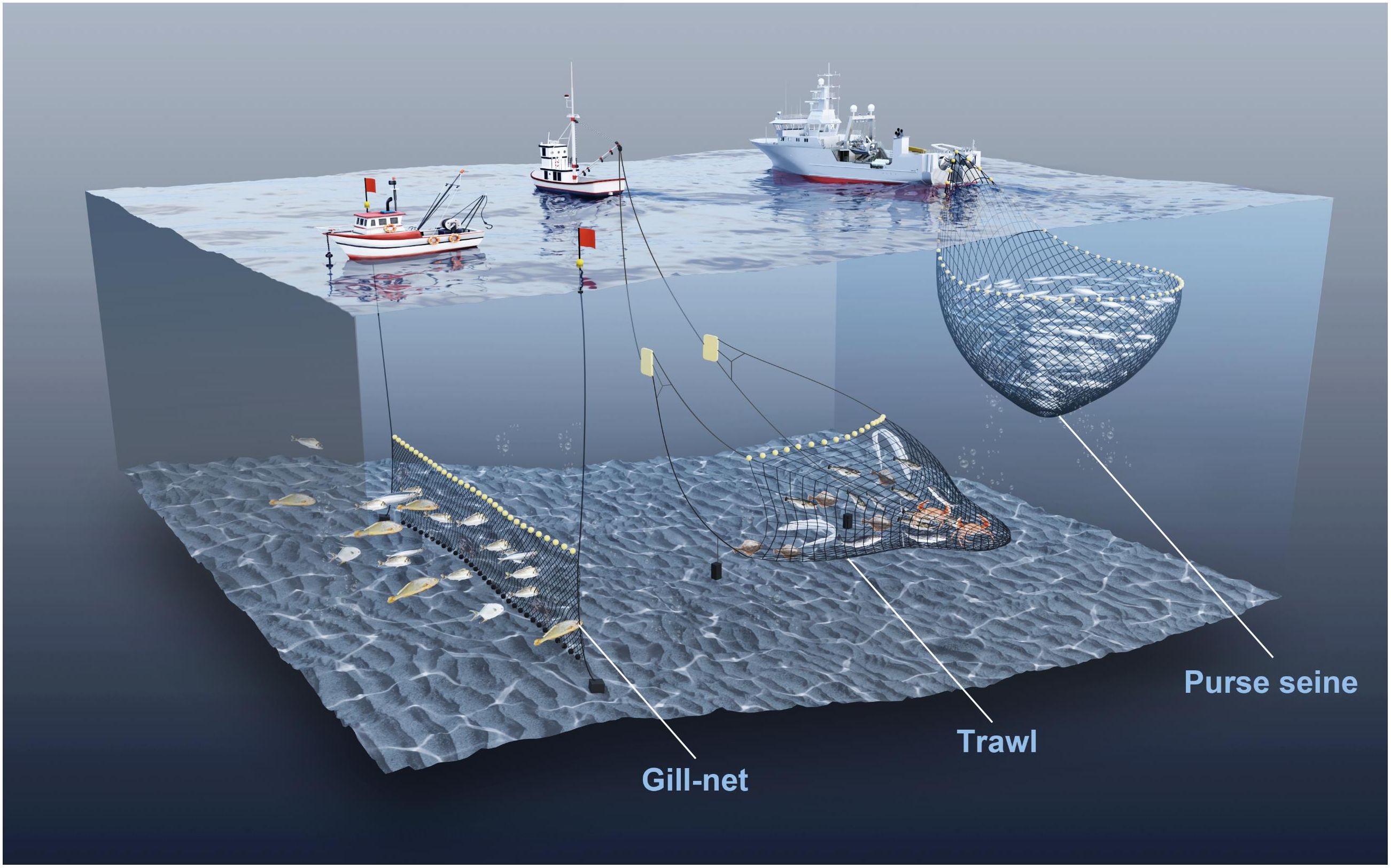
Figure 1. Operating principle of gillnet, trawl, and purse seine and spatial distribution of main catches.

3.1.2 Beidou VMS and AIS data preprocessing

Due to data errors and redundancy during the transmission of VMS and AIS data, it is necessary to clear the erroneous and redundant data. Erroneous data mainly includes situations such as missing data and abnormal data. Data abnormalities mainly include abnormal speed and heading (such as speed>50 knots, heading greater than 360°), as well as situations where the maritime mobile service identity (MMSI) is less than nine digits. Redundant data includes two or more identical records of the same vessel. Error data and redundant data need to be deleted, whereafter key data, such as MMSI, speed, course, longitude, latitude, and time, should be extracted. In AIS data, the units of speed and course are 0.1 knots and 0.1°, respectively. The speed and course must be divided by 10, which is consistent with the Beidou VMS data. Voyages are divided according to the time interval, longitude, latitude, and change in speed of two consecutive data sent by a fishing vessel. In this study, the time interval of more than one day, constant or minimal change of longitude and latitude, and zero speed were taken as the criteria for dividing voyages, which were filtered to eliminate invalid voyages.

3.1.3 Feature set selection

According to the literature (Huang et al., 2019) and Beidou VMS data statistics, the three types of fishing vessels have large differences in longitude, latitude, speed, and course (see Supplementary Figure S2). Typical trajectories, speed changes, and frequency distributions of gillnets, trawls, and purse seines are shown in Supplementary Figures S3–S5, respectively. Therefore, 203 features related to longitude, latitude, speed, and course were selected, as shown in Table 1. We divide the vessel’s speed into four intervals: stopping or movement caused by wind and wave (0, 0.5), low-speed fishing (0.5, 2.5), medium-speed fishing (2.5, 6), and navigation (6, 12) based on the speed changes and frequency distribution map.

Table 1

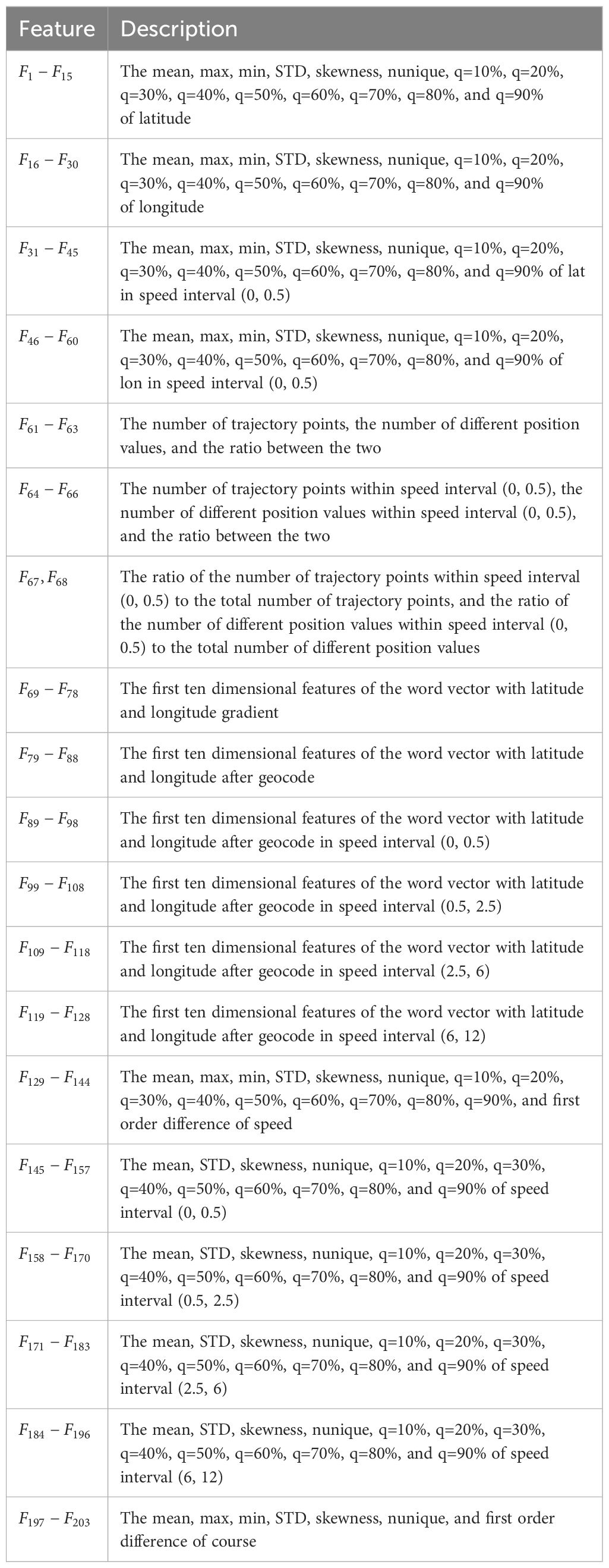
Table 1. Features description.

For longitude and latitude, conventional statistical features such as mean, max, min, standard deviation (STD), skewness, the number of different values (nunique), and nine quantiles (q) were first selected as features ($F_1-F_{30}$). A complete voyage usually includes some trajectory points of the vessel when it is moored in the port. Under the action of wind and waves, these trajectory points also have small velocities, similar to the operating speed of the gillnet. Therefore, we selected the mean, max, min, STD, skewness, the count of unique values (nunique), and nine quantiles of longitude and latitude with speed less than 0.5 knots as features ($F_{31}-F_{60}$). The number of trajectory points for each ship, the number of different position values, and the ratio between the two were counted as features ($F_{61}-F_{63}$). We also counted the number of trajectory points with a speed of less than 0.5 knots, the number of different position values with a speed less than 0.5 knots, and the ratio between the two as the feature $F_{64}-F_{66}$. The ratio of the number of trajectory points within the speed range of 0-0.5 knots to the total number of trajectory points and the ratio of the number of different position values within the speed range of 0-0.5 knots to the total number of different position values are used as the feature ($F_{67},F_{68}$). Moreover, the gradients of longitude and latitude were calculated, and the word vector matrix of the gradients was obtained using the term frequency-inverse document frequency (TF-IDF). Then, we used singular value decomposition (SVD) to reduce the dimensionality of the matrix, retaining the most important first ten-dimensional features ($F_{69}-F_{78}$). In addition, the geohash method was used to geocode longitude and latitude, and then TF-IDF and SVD were used to extract ten-dimensional features. Divide the longitude and latitude after geocoded according to four speed intervals, and repeat the above operation to obtain the feature ($F_{89}-F_{128}$).

For speed, we selected mean, max, min, STD, skewness, nunique, nine quantiles, and first-order difference as features ($F_{129}-F_{144}$). The mean, variance, skewness, nunique, and nine quantiles of the speed in the four-speed intervals were also counted as characteristics ($F_{145}-F_{196}$).

For the course, we selected mean, max, min, STD, skewness, nunique, and first-order differential statistical features as features ($F_{197}-F_{203}$).

Not all features are beneficial for the model, so in the subsequent model construction process, we will calculate the importance of each feature and screen the features.

3.1.4 Fishing vessel behavior recognition model construction

LightGBM is an open source and efficient gradient-boosting decision tree (GBDT) algorithm developed by Microsoft (Wang et al., 2017), which belongs to Boosting in integrated learning (Grabner and Bischof, 2006). It contains multiple weak classifiers and uses the addition model to continuously optimize and reduce the training residual of the previous weak classifier to achieve classification and regression. As the LightGBM algorithm presents advantages of higher accuracy, faster training speed, big data processing ability, and supporting parallel learning (Al Daoud, 2019), it was selected to construct a fishing vessel behavior recognition model.

For the 15166 fishing vessels data of the Beidou VMS, we randomly divided the dataset into five equally sized subsets. Four of these subsets were used for model training, while the remaining one was set aside for testing. This process was repeated five times, with a different subset selected as the test set each time and the others used for training. Secondly, trawl, purse seine, and gillnet were mapped to three labels: 0, 1, and 2, respectively, and thirdly, normalized the features of the preprocessed training set to eliminate the impact of unit and scale differences between features and accelerate the convergence rate of the model. The Sklearn library in Python was then used to perform principal component analysis, feature importance assessment, and call and evaluate the model. The main parameter settings of the algorithm are shown in Table 2.

Table 2

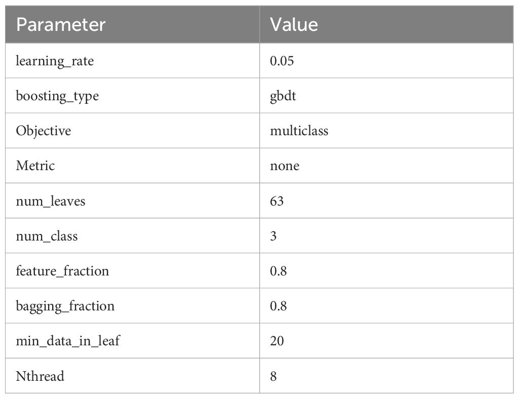
Table 2. LightGBM main parameter settings.

We selected 203 features to construct the model (Table 1) and used the average information gain brought by a feature during splitting as a measure of feature importance. The higher the gain, the greater the impact of this feature on the training of the model, and the equation is as follows:

$\begin{array}{ll}Gain= \frac{1}{2}\left[\frac{G_L^2}{H_L+\lambda }+\frac{G_R^2}{H_R+\lambda }-\frac{{(G_L+G_R)}^2}{H_L+H_R+\lambda }\right]-\gamma & (1)\end{array}$

where $G_L$ and $G_R$ respectively represent the sum of the first derivative of the loss function on the left and right nodes, $H_L$ and $H_R$ correspond to the sum of the second derivative of the loss function on the left and right nodes, $\lambda$ is the hyperparameter of the regularization, and $\gamma$ is regularization on the additional leaf.

Then, we sorted the features in descending order of importance, deleted them one by one from the lowest importance, and input the feature set after deletion into the model for training. The model with 91 deleted features has the highest F1-score and accuracy in the training set, so the top 112 features were ultimately retained for training the model. The retained features and their importance are shown in Supplementary Figure S6.

3.1.5 Fishing vessel behavior recognition model validation

The model validation was based on five-fold cross-validation. The accuracy, precision, recall, and F1-score were used as evaluation indicators for the model. We averaged the five performance evaluations to derive the final result. The five-fold cross-validation results are listed in Table 3, where the accuracy of behavior recognition of fishing vessels indicates the proportion of fishing vessels with correct classification in the total fishing vessels. The average recall of behavior recognition of fishing vessels indicates the proportion of a fishing vessel with correct classification to the real number of such fishing vessels. The average precision of behavior recognition of fishing vessels refers to the proportion of a fishing vessel with correct classification in the total predicted number of such fishing vessels. The average F1-score of the behavior type identification of fishing vessels is the harmonic average of the precision and recall (Chicco and Jurman, 2020), and higher precision and recall are preferred. However, sometimes they show contradictions between them. The F1-score is a comprehensive consideration of both. The results showed that the fishing vessel behavior recognition model used in this study had high accuracy, recall, precision, and F1-score, and could accurately identify the types of fishing vessel behavior.

Table 3

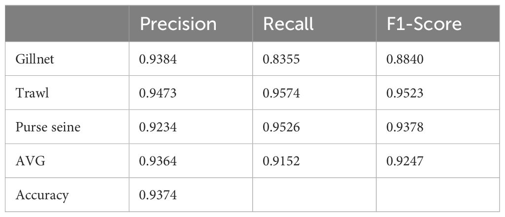
Table 3. Fishing vessel behavior recognition model verification results.

3.1.6 Fishing time qualitative analysis

Fishing intensity is related to the fishing time, degree of fishing mechanization, effective fishing capacity of vessels, horsepower, labor, and nets. Under the same fishing methods and other conditions, a longer fishing time means a greater fishing intensity. High intensity fishing operations can lead to the depletion of fishery resources. Therefore, we qualitatively evaluate fishing time to measure the fishing intensity of different behavior types of fishing vessel.

The behavior recognition model of fishing vessels was applied to 6358 fishing vessels in Zhejiang Province in the East China Sea, and the data with prediction probabilities of the three types of fishing vessel behaviors <0.4 were identified as abnormal behaviors. The behavior type data set after removing abnormal fishing vessel data were used for subsequent qualitative assessment of fishing time. The speed and course features of fishing status are different from the navigation status. The fishing track of each voyage was extracted using the change of speed and course (Deng et al., 2005; Lee et al., 2010), and then counted the fishing time of fishing vessels with three types of behavior (gillnet, trawl, and purse seine) in 0.25° × 0.25° longitude and latitude grids daily from September to December 2021.

According to the cumulative fishing time per unit longitude and latitude grid of fishing vessels of each behavior type every day in four months, the unit longitude and latitude grid where the first 30% of fishing time was located was designated as the low fishing time area, 30–60% was the medium fishing time area, and the last 40% was the high fishing time area. Figure 2 shows the qualitative evaluation result of daily average fishing time of different fishing vessel behaviors in Zhejiang Province from September to December 2021.

Figure 2

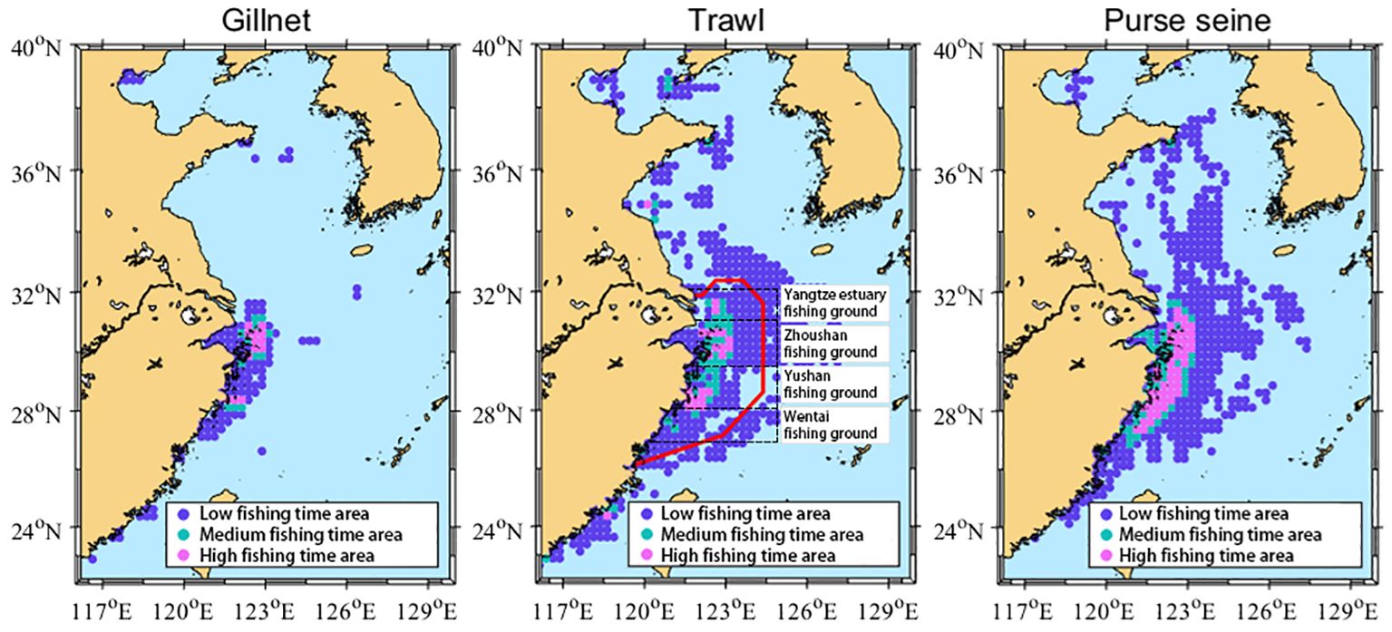
Figure 2. Fishing time qualitative evaluation of fishing vessels of three behavior types in Zhejiang province from September to December 2021. The study area is included within the red line.

As the main operation areas of fishing vessels were concentrated in the Zhoushan, Yushan, and Wentai fishing grounds, we selected the area surrounded by the red line in Figure 2 as the research area. Then, based on the qualitative assessment results and big data of the marine environment, we used the decision tree algorithm to establish a coupling model of fishing time and big marine environment data.

3.2 Study on coupling model of fishing time and marine environment big data

The coupling model of fishing time and marine environment uses fishing time data qualitatively evaluated in section 3.1.6 and marine environment data including chl-a, SST, SLA, sea surface wind, sea surface current, and water depth. Using the aforementioned data, a coupled model was constructed to fine predict fishing times of three types of fishing vessels. The research on the coupling model of fishing time and marine environment big data includes the following steps.

3.2.1 Marine environmental data preprocessing

The missing chl-a concentration from September to December 2021 was replaced with the monthly average chl-a concentration data from 2015 to 2021 and the time resolution of all marine environmental elements (including chl-a, SST, SLA, sea surface wind, sea surface current and water depth) was then unified to days and the data with multiple values in a day were averaged. The spatial resolution of all marine environmental elements was unified to 0.25° × 0.25°, and down-sampling was conducted for chl-a and water depth data.

3.2.2 Training sample production

The qualitative assessment results of fishing time for each type of fishing vessel behavior were divided by day (three types × 122 days = 366 documents in total). The longitude and latitude grid point of low fishing time area was labeled as 1, that of medium fishing time area was labeled as 2, and that of high fishing time area was labeled as 3. This study used 12 marine environmental features as the input of the model, including longitude (Lon), latitude (Lat), chl-a, SST, SLA, sea surface wind (U10, V10, $\sqrt[2]{U{10}^2+V{10}^2}$), surface current (u, v, $\sqrt[2]{u^2+v^2}$), and water depth. We randomly divided the 122 days into five equally sized subsets. Four of these subsets were used for model training, while the remaining one was set aside for testing. This process was repeated five times, with a different subset selected as the test set each time and the others used for training.

3.2.3 Fishing time and marine environment coupling model construction

The decision tree is a commonly used supervised learning classification algorithm, which adopts a top-down recursive strategy to establish a relationship model between multiple and response variables (Song and Ying, 2015; Raju and Laxmi, 2020). The decision tree has the advantages of simplicity and efficiency, and its comprehensibility is superior to that of black box models (such as neural networks) (Kotsiantis, 2013). In this study, we used the fine trees, optimization trees, and bagged trees in the Matlab classification learner to construct the model. A fine tree is a decision tree with many leaves used for fine classification (the maximum number of splits is 100). An optimizable tree is a decision tree classifier that can optimize super parameters. The bagged tree is a self-service aggregation of fine decision trees. In addition, we also tried to use two common neural networks: convolutional neural networks (CNN) and long short-term memory (LSTM). For each type of fishing vessel behavior, the marine environment data were taken as the variable, and each grid point’s fishing time category was taken as the response variable. The coupling model of fishing time and marine environment big data for three types of behavior was established accordingly.

3.2.4 Fishing time and marine environment coupling model validation

The validation of coupling model of fishing time and marine environment big data was based on five-fold cross-validation. The accuracy, precision, recall, and F1-score were used as evaluation indicators for the model. We averaged the five performance evaluations to derive the final result. The five-fold cross-validation results (Table 4) show that the precision, recall, F1-score, and accuracy of the bagged tree algorithm were mostly higher than those of the fine tree, optimizable tree, CNN, and LSTM. The average precision, recall, F1-score, and accuracy of the coupling model constructed by bagged tree were 0.5790, 0.5655, 0.5722, and 0.6216, respectively. The above results show that the coupling model of fishing time and marine environment big data constructed by bagged tree is superior to the other four methods. Here, we ultimately chose the bagging tree to build the coupling model.

Table 4

Table 4. Fishing time and marine environment coupling model verification results.

3.3 Spatio-temporal prediction of suspected high intensity fishing operation areas

The time-space prediction of suspected high intensity fishing operation areas is based on the coupling model mentioned above, as well as marine environment forecast data including chl-a, SST, SLA, sea surface wind, sea surface current, and water depth forecast data. The detailed steps are as follows: (1) preprocessing marine environment forecast data and unifying the time resolution of all marine elements to daily and spatial resolution to 0.25° × 0.25°. (2) Using the marine environment forecast data as the input of the coupling model of fishing time and marine environment to search for daily suspected high intensity fishing operation areas in the coming days.

4 Results and discussion

This study is mainly divided into four parts. First part analyzed the results of fishing vessel behavior recognition in Zhejiang Province. The second and third parts verified the accuracy of the coupling model by analyzing the fishing time and the relationship between fishing time and SST. The final part realized and analyzed fine spatio-temporal fishing time prediction.

4.1 Analysis of fishing vessel behaviors (taking fishing vessels in Zhejiang province as an example)

This paper applied a fishing vessel behavior recognition model to fishing vessels in Zhejiang Province. The 6538 fishing vessel data were divided into 10607 voyages as input to the model. The data with prediction probabilities of the three types of fishing vessel behaviors <0.4 were identified as abnormal behaviors. The distribution of fishing vessel behavior in Zhejiang Province from September to December 2021 was shown in Figure 3.

Figure 3

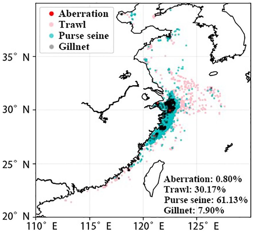
Figure 3. Distribution of fishing vessel behaviors in Zhejiang Province.

From the fishing vessel behavior recognition results, it can be found that in the fishing vessel in Zhejiang Province, the proportion of trawl voyages is 30.17%, the proportion of purse seine voyages is 61.13%, the proportion of gillnet voyages is 7.9%, and the proportion of abnormal voyages is 0.8%. The high proportion of purse seine voyages may be due to two reasons: (1) In the collected fishing vessel data in Zhejiang Province, the number of purse seine fishing vessels is relatively large; (2) A purse seine fishing vessel is divided into more voyage data than trawlers and gillnet fishing vessels.

From Figure 3, it can also be seen that in the collected data, the fishing areas where fishing vessels catch are mainly concentrated in Zhoushan Fishing Ground, Yushan Fishing Ground, and Wentai Fishing Ground along the Zhejiang coast. A small number of fishing vessels go to the Yellow Sea, Bohai Sea, and South China Sea to fish. The abnormal behavior of fishing vessels mainly occurs in Zhoushan fishing grounds, and the reasons for its occurrence may be: (1) Fishing vessels engage in non fishing vessel behaviors, such as transportation, resource investigation, illegal passenger transportation, and illegal trading; (2) Fishing vessels are engaged in more than one type of fishing operation, resulting in two or more types of fishing vessel behaviors in the AIS trajectory, which may cause the probability of three types of fishing vessel behaviors are less than 0.4; (3) Some fishing vessels data are incomplete, resulting in biased extraction of fishing features.

More historical trajectory data of a suspicious fishing vessel can be queried through relevant AIS data (MMSI number, time, etc.), in order to conduct a more comprehensive and detailed analysis of the vessel’s behavior, determine whether there are activities related to national security and damage to the marine ecological environment, such as illegal surveying and fishing, and regulate fishing vessel behaviors.

4.2 Analysis of fishing time (grid)

Using the coupled model constructed by bagging trees to estimate fishing time for the marine environment big data in the testing set in the East China Sea area, we selected two days to present in the paper. The predicted results and actual fishing time of gillnet, trawl, and purse seine on December 4 and 10, 2021, are depicted in Figure 4.

Figure 4

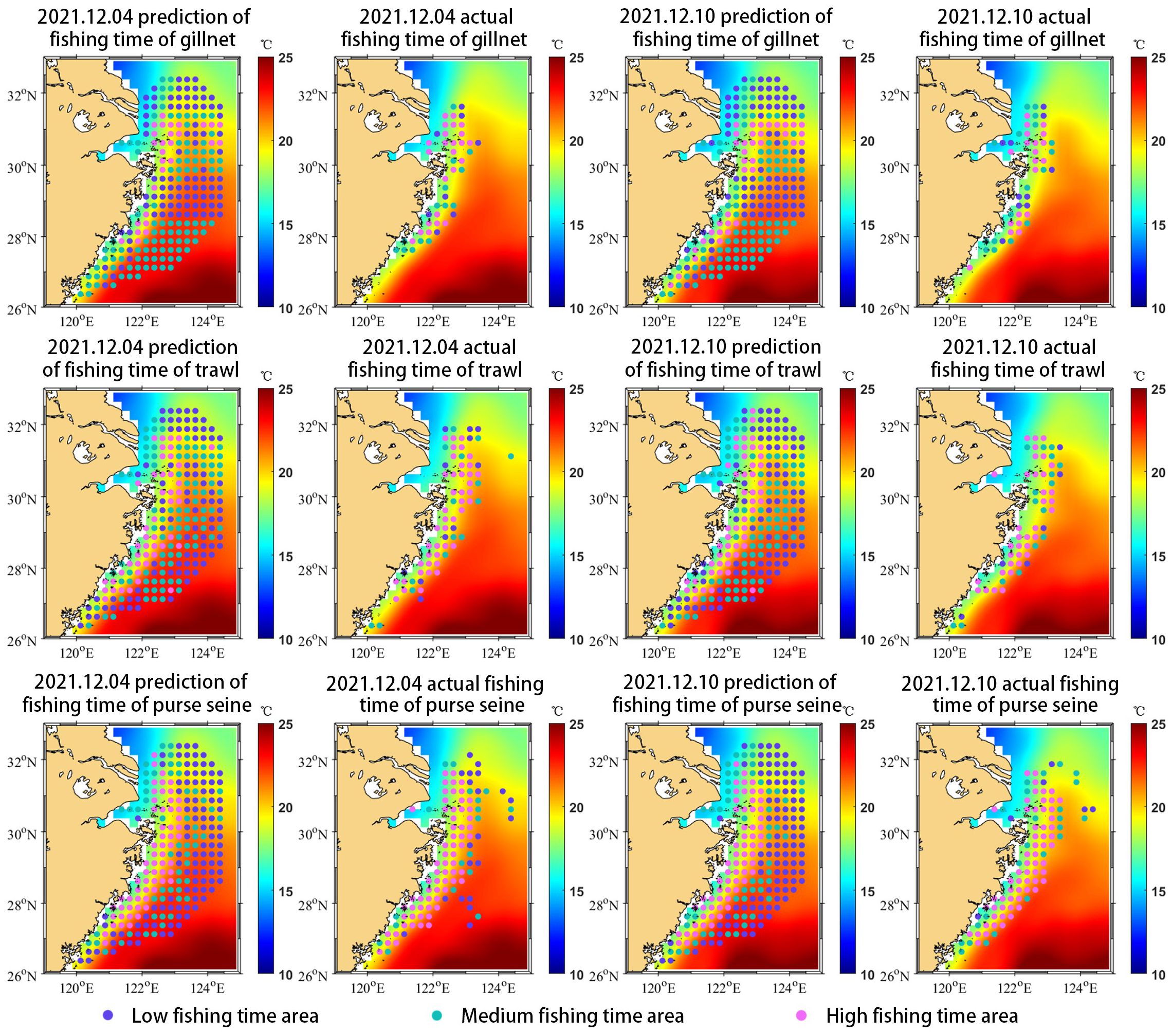
Figure 4. Predicted and actual fishing time in the East China Sea (The background is the sea surface temperature (SST) of the day).

The predicted and actual fishing time of the three fishing types (Figure 4) indicate that the existing data and the predicted fishing time of this data point are well matched, and the coupling model is relatively accurate. The areas with high fishing time of gillnets, trawls, and purse seines were mainly concentrated in the Zhoushan, Yushan, and Wentai fishing grounds and other sea areas. Fishery supervision can be efficiently focused on the areas with medium and high fishing time, such as appropriately reducing fishing intensity of a certain fishing vessel type to reduce the pressure on the main species caught by this fishing vessel type, and preventing illegal fishing.

4.3 Relationship between fishing time and SST

Among many environmental factors, sea temperature is one of the critical factors affecting the spatial distribution and abundance of most fishery resources (Southward et al., 1995). We predicted the fishing time of the East China Sea on December 4, 2021 and discussed the relationship between fishing time and SST. The SST was approximately 15–23°C in the predicted high fishing time area of the three types of fishing vessel behaviors in the East China Sea, changing more substantially than in the predicted low and medium fishing time areas in general (Figure 4). According to literature (Hickox et al., 2000), there is a Zhejiang-Fujian Front along the coast of Zhejiang and Fujian in winter. The horizontal gradient of temperature, salinity, and other marine elements in the frontal zones is large, accompanied by the strengthening of vertical circulation, which leads to nutrient substance enrichment and provides abundant food for phytoplankton (Belkin et al., 2009; Bost et al., 2009). Therefore, the frontal zones often form potential fishing grounds (Polovina et al., 2000; Zainuddin et al., 2004). The identified high fishing time area was located in the Zhejiang-Fujian Front area. Liu and Yu (2018) also showed that higher resources are distributed in the Northern South China Sea near the study area with SST of 17–24°C in winter, which is consistent with the SST of the identified high fishing time area.

In winter, the sea temperature in the continental shelf area of the East China Sea is vertically uniform, and the strength of the thermocline is mostly <0.1°C/m (Hao et al., 2012). The water depth in the high fishing time area is mostly within 50 m, and the temperature difference between the sea surface and bottom is small (usually less than 5°C).

Small yellow croakers represent important economic fish, and live near the bottom of the East China Sea. During the autumn and winter floods from early September to the end of December, the fishing methods mainly comprise gillnets and trawls. The sea bottom temperature estimated from SST in the high fishing time area of gillnets and trawls was consistent with the temperature preference of small yellow croakers (Cheung et al., 2009).

Mackerels are one of the main species caught in purse seines in the East China Sea. Mackerels inhabit the upper and middle sea level, where the sea temperature is generally 10–27°C (Cheung et al., 2013). As sea temperature is the main, rather than the only factor affecting fishery resources, other marine environmental factors such as abnormal sea surface height and chlorophyll also have an impact on fishery resources (Solanki et al., 2015). This may explain why the SST in high, medium, and low fishing time areas was within the range of suitable habitat water temperature for mackerel, but the fishing time in the areas differ (Figure 4).

4.4 Spatio-temporal dynamic predict of fishing time

The historical marine environment data were used to build and verify the coupling model of fishing time. The coupling mode was then used to predicted fishing time within one week according to different fishing vessel behaviors. Figure 5 presents the prediction result on July 29, 2022, when the East China Sea is in the closed fishing season.

Figure 5

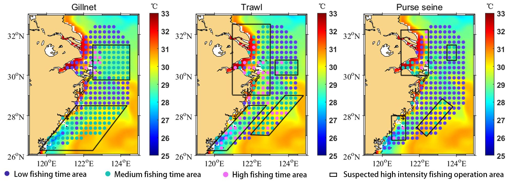
Figure 5. Prediction results of fishing time in the East China Sea on July 29, 2022.

The following conclusions can be drawn from Figure 5:

1. Suspected high intensity fishing operation area of gillnet (the medium and high fishing time area) in the East China Sea predicted on July 29 was mainly located in the Zhoushan and Wentai fishing grounds, and the SST was mainly 28–31°C. The scope was consistent with the high abundance area of main gillnet fishing objects, such as small yellow croaker and yellow crucian carp, in the East China Sea in summer (Cheung et al., 2009; Liu, 2004). The range of medium and high fishing time area predicted for gillnet was much larger than that for trawl and purse seine, mainly because the data of gillnet outside 123°E was scarce and far less than that of trawl and purse seine.

2. The suspected high intensity fishing operation of trawl predicted on July 29 was mainly located in Zhoushan and Wentai fishing grounds, and the SST was mainly 27–33°C. This scope was consistent with the high abundance area of main trawling objects, such as small and large yellow croaker and Benthosema pterotum, in the East China Sea in summer (Cheung et al., 2009; Wang et al., 2020; Xu et al., 2022). As gillnets and trawls mainly catch bottom and near bottom fish, the vertical temperature change of the East China Sea shelf sea area in summer was substantial (Hao et al., 2012), and the difference between sea bottom and surface temperatures was large, regardless of whether the temperature range was consistent.

3. The purse seine suspected high intensity fishing operation predicted on July 29 was mainly located in Zhoushan and Wentai fishing grounds, and the SST was mainly 27–33°C. The suspected high intensity fishing operation of purse seine was consistent with the summer distribution area of main purse seine objects, such as Chub mackerel, in the East China Sea (Chen et al., 2009; Yu et al., 2018), and its temperature included the optimum temperature of mackerel in summer (Chen et al., 2009).

Additionally, we compared our forecasted results with the fishing times available on the Global Fishing Watch website for July 29, 2022. Global Fishing Watch website (Figure 6) shows that areas of high fishing time are observed in the vicinity of (122-123°E, 30-31°N), (120°E, 26.5°N), (121.5°E, 27.5°N), and (123.5°E, 27.5°N), which generally align with our predictions of areas with high fishing time (Figure 5).

Figure 6

Figure 6. The fishing time provided by the Global Fishing Watch website on July 29, 2022.

The above analysis shows that the refined grid predict of the prediction model for the suspected high intensity fishing operation area was generally consistent with the traditional fishing grounds and Global Fishing Watch. The results can provide a space-time reference for setting key patrol areas during the closed fishing season to facilitate the supervision of fishing vessels in the fishing grounds, achieve refined protection of fishery resources, and improve the efficiency of fishery supervision.

5 Conclusions

Overfishing, bycatch, and other anthropogenic threats may lead to the destruction of fragile habitats and substantial losses of marine life. Most fish stocks worldwide are caught at maximum sustainable or unsustainable rates. Finding effective regulatory measures to protect marine fishery resources and the ecological environment is extremely urgent. In response to the difficult issues of “searching for high intensity fishing operation area, and classifying and supervising fishing vessels according to their types” to achieve effective fisheries regulation, this study attempts to build a prediction model for fishing time based on AIS and marine environment big data, to achieve fishing vessel fishing regulation, qualitative assessment of fishing time, and refined prediction of high intensity fishing operation areas. The summary of this study is as follows:

1. The average accuracy, recall, precision, and F1-score of the fishing vessel behavior recognition model we constructed are greater than 0.9, indicating that our model can accurately identify the behavior of fishing vessels.

2. The results of the qualitative assessment of fishing time showed that areas with high fishing time mainly occurred in Zhoushan, Yushan, and Wentai fishing grounds. Fisheries regulation can focus on areas with medium to high fishing time, appropriately reducing the effort of fishing vessels of certain types, reducing pressure on the main fishing species of such vessels, and preventing overfishing.

3. We used algorithms such as fine optimizable and bagging trees to establish a coupling model between fishing time and marine environment big data. The results show that the bagging tree algorithm is superior. Subsequently, we explored the relationship between SST and fishing time to further validate the model results.

4. Finally, we established a spatio-temporal model in the East China Sea to predict fishing time during the closed fishing season. The prediction results generally conform to the distribution of traditional fishery resources in the East China Sea and the fishing efforts provided by the Global Fishing Watch, and provide a reference basis for searching for high intensity fishing operation areas.

However, because some of the data we used in this study were from AIS fishing vessels in Zhejiang Province and the data volume was small, we could only conduct analysis and predict fishing time in the East China Sea. With sufficient AIS data of fishing vessels, prediction of pelagic fishing time in the open sea can be performed to strengthen supervision and management of pelagic fishing vessels during self-help fishing closures, prevent illegal operations by pelagic fishing vessels, promote conservation of fishery resources in the open sea, and promote high-quality development of pelagic fisheries.

Data availability statement

The original contributions presented in the study are included in the article/Supplementary Material. Further inquiries can be directed to the corresponding authors.

Author contributions

YZ: Writing – original draft, Validation, Software, Methodology. PC: Writing – review & editing, Supervision, Methodology, Conceptualization. GZ: Writing – review & editing. DW: Writing – review & editing, Formal analysis. JY: Writing – review & editing, Resources. XL: Writing – review & editing, Investigation. DL: Writing – review & editing, Investigation.

Funding

The author(s) declare financial support was received for the research, authorship, and/or publication of this article. This work was supported by the China High-Resolution Earth Observation System Program under Grant 41-Y30F07-9001-20/22 and the Zhejiang Provincial Natural Science Foundation of China under Grant No. LR21D060002.

Acknowledgments

We thank Prof. Guoqi Han for critical ideas on this article.

Conflict of interest

The authors declare that the research was conducted in the absence of any commercial or financial relationships that could be construed as a potential conflict of interest.

Publisher’s note

All claims expressed in this article are solely those of the authors and do not necessarily represent those of their affiliated organizations, or those of the publisher, the editors and the reviewers. Any product that may be evaluated in this article, or claim that may be made by its manufacturer, is not guaranteed or endorsed by the publisher.

Supplementary material

The Supplementary Material for this article can be found online at: https://www.frontiersin.org/articles/10.3389/fmars.2024.1421188/full#supplementary-material

References

Al Daoud E. (2019). Comparison between XGBoost, LightGBM and CatBoost using a home credit dataset. Int. J. Comput. Inf. Eng. 13, 6–0. doi: 10.5281/zenodo.3607805

Crossref Full Text | Google Scholar

Belkin I. M., Cornillon P. C., Sherman K. (2009). Fronts in large marine ecosystems. Prog. Oceanography 81, 223–236. doi: 10.1016/j.pocean.2009.04.015

Crossref Full Text | Google Scholar

Bost C. A., Cotté C., Bailleul F., Cherel Y., Charrassin J. B., Guinet C., et al. (2009). The importance of oceanographic fronts to marine birds and mammals of the southern oceans. J. Mar. Syst. 78, 363–376. doi: 10.1016/j.jmarsys.2008.11.022

Crossref Full Text | Google Scholar

Chen X., Li G., Feng B., Tian S. (2009). Habitat suitability index of Chub mackerel (Scomber japonicus) from July to September in the East China Sea. J. Oceanography 65, 93–102. doi: 10.1007/s10872-009-0009-9

Crossref Full Text | Google Scholar

Cheung W. W., Lam V. W., Sarmiento J. L., Kearney K., Watson R., Pauly D. (2009). Projecting global marine biodiversity impacts under climate change scenarios. Fish Fisheries 10, 235–251. doi: 10.1111/j.1467-2979.2008.00315.x

Crossref Full Text | Google Scholar

Cheung W. W., Watson R., Pauly D. (2013). Signature of ocean warming in global fisheries catch. Nature 497, 365–368. doi: 10.1038/nature12156

PubMed Abstract | Crossref Full Text | Google Scholar

Chicco D., Jurman G. (2020). The advantages of the Matthews correlation coefficient (MCC) over F1 score and accuracy in binary classification evaluation. BMC Genomics 21, 1–13. doi: 10.1186/s12864-019-6413-7

Crossref Full Text | Google Scholar

Cimino M. A., Anderson M., Schramek T., Merrifield S., Terrill E. J. (2019). Towards a fishing pressure prediction system for a western Pacific EEZ. Sci. Rep. 9, 1–10. doi: 10.1038/s41598-018-36915-x

PubMed Abstract | Crossref Full Text | Google Scholar

Costello M. J., Coll M., Danovaro R., Halpin P., Ojaveer H., Miloslavich P. (2010). A census of marine biodiversity knowledge, resources, and future challenges. PloS One 5, e12110. doi: 10.1371/journal.pone.0012110

PubMed Abstract | Crossref Full Text | Google Scholar

Crowder L. B., Hazen E. L., Avissar N., Bjorkland R., Latanich C., Ogburn M. B. (2008). The impacts of fisheries on marine ecosystems and the transition to ecosystem-based management. Annu. Rev. Ecology Evolution Systematics 39, 259–278. doi: 10.1146/annurev.ecolsys.39.110707.173406

Crossref Full Text | Google Scholar

Davies B. F., Holmes L., Bicknell A., Attrill M. J., Sheehan E. V. (2022). A decade implementing ecosystem approach to fisheries management improves diversity of taxa and traits within a marine protected area in the UK. Diversity Distributions 28, 173–188. doi: 10.1111/ddi.13451

Crossref Full Text | Google Scholar

Deng R., Dichmont C., Milton D., Haywood M., Vance D., Hall N., et al. (2005). Can vessel monitoring system data also be used to study trawling intensity and population depletion? The example of Australia’s northern prawn fishery. Can. J. Fisheries Aquat. Sci. 62, 611–622. doi: 10.1139/f04-219

Crossref Full Text | Google Scholar

EC Reg. (2008). 2008/56 Establishing a Framework for Community Action in the Field of Marine Environmental Policy (Marine Strategy Framework Directive). Available online at: http://eur-lex.europa.eu/legal-content/EN/TXT/?uri=CELEX:32008L0056 (Accessed: June 25, 2008).

Google Scholar

Eddy C., Brill R., Bernal D. (2016). Rates of at-vessel mortality and post-release survival of pelagic sharks captured with tuna purse seines around drifting fish aggregating devices (FADs) in the equatorial eastern Pacific Ocean. Fisheries Res. 174, 109–117. doi: 10.1016/j.fishres.2015.09.008

Crossref Full Text | Google Scholar

Ferrà C., Tassetti A. N., Grati F., Pellini G., Polidori P., Scarcella G., et al. (2018). Mapping change in bottom trawling activity in the Mediterranean Sea through AIS data. Mar. Policy 94, 275–281. doi: 10.1016/j.marpol.2017.12.013

Crossref Full Text | Google Scholar

Fonseca P., Martins R., Campos A., Sobral P. (2005). Gill-net selectivity off the Portuguese western coast. Fisheries Res. 73, 323–339. doi: 10.1016/j.fishres.2005.01.015

Crossref Full Text | Google Scholar

Gerber L. R., Kareiva P. M., Bascompte J. (2002). The influence of life history attributes and fishing pressure on the efficacy of marine reserves. Biol. Conserv. 106, 11–18. doi: 10.1016/S0006-3207(01)00224-5

Crossref Full Text | Google Scholar

Grabner H., Bischof H. (2006). “On-line Boosting and Vision,” in 2006 IEEE Computer Society Conference on Computer Vision and Pattern Recognition (CVPR'06). New York, NY, USA: IEEE. vol. 1, pp. 260–267, doi: 10.1109/CVPR.2006.215

Crossref Full Text | Google Scholar

Halpern B. S., Frazier M., Potapenko J., Casey K. S., Koenig K., Longo C., et al. (2015). Spatial and temporal changes in cumulative human impacts on the world’s ocean. Nat. Commun. 6, 1–7. doi: 10.1016/j.compchemeng.2011.01.009

Crossref Full Text | Google Scholar

Hao J., Chen Y., Wang F., Lin P. (2012). Seasonal thermocline in the China Seas and northwestern Pacific Ocean. J. Geophysical Research: Oceans 117, C02022. doi: 10.1029/2011JC007246

Crossref Full Text | Google Scholar

Harati-Mokhtari A., Wall A., Brooks P., Wang J. (2007). Automatic Identification System (AIS): data reliability and human error implications. J. Navigation 60, 373–389. doi: 10.1017/S0373463307004298

Crossref Full Text | Google Scholar

Hickox R., Belkin I., Cornillon P., Shan Z. (2000). Climatology and seasonal variability of ocean fronts in the East China, Yellow and Bohai Seas from satellite SST data. Geophysical Res. Lett. 27, 2945–2948. doi: 10.1029/1999GL011223

Crossref Full Text | Google Scholar

Huang H., Hong F., Liu J., Liu C., Feng Y., Guo Z. (2019). FVID: fishing vessel type identification based on VMS trajectories. J. Ocean Univ. China 18, 403–412. doi: 10.1007/s11802-019-3717-9

Crossref Full Text | Google Scholar

Jackson J. B. C., Kirby M. X., Berger W. H., Bjorndal K. A., Botsford L. W., Bourque B. J., et al. (2001). Historical overfishing and the recent collapse of coastal ecosystems. Science 293, 629–637. doi: 10.1126/science.1059199

PubMed Abstract | Crossref Full Text | Google Scholar

Jin X., Tang Q. (1996). Changes in fish species diversity and dominant species composition in the Yellow Sea. Fisheries Res. 26, 337–352. doi: 10.1016/0165-7836(95)00422-X

Crossref Full Text | Google Scholar

Jones P. J. (2002). Marine protected area strategies: issues, divergences and the search for middle ground. Rev. Fish Biol. Fisheries 11, 197–216. doi: 10.1023/A:1020327007975

Crossref Full Text | Google Scholar

Kotsiantis S. B. (2013). Decision trees: a recent overview. Artif. Intell. Rev. 39, 261–283. doi: 10.1007/s10462-011-9272-4

Crossref Full Text | Google Scholar

Lee J., South A. B., Jennings S. (2010). Developing reliable, repeatable, and accessible methods to provide high-resolution estimates of fishing-effort distributions from vessel monitoring system (VMS) data. ICES J. Mar. Sci. 67, 1260–1271. doi: 10.1093/icesjms/fsq010

Crossref Full Text | Google Scholar

Li L. Z., Tang J. H., Xiong Y., Huang H. L., Wu L., Shi J. J., et al. (2017). “Mesh size selectivity of the gillnet in East China Sea,” in IOP Conference Series: Earth and Environmental Science, Vol. 77, 012013. doi: 10.1088/1755-1315/77/1/012013

Crossref Full Text | Google Scholar

Liu Y. (2004). A study on the distribution of Setipinna taty in the East China Sea. Mar. Fisheries 26, 255–260.

Google Scholar

Liu Z., Yu J. (2018). Response of Spatio-temporal distribution of fishery resources to marine environment in the Northern South China Sea. Anim. Husbandry Feed Sci. 10, 311–320. doi: 10.19578/j.cnki.ahfs.2018.05-06.009

Crossref Full Text | Google Scholar

Lubchenco J., Palumbi S. R., Gaines S. D., Andelman S. (2003). Plugging a hole in the ocean: the emerging science of marine reserves. Ecol. Appl. 13, S3–S7. doi: 10.1890/1051-0761(2003)013[0003:PAHITO]2.0.CO;2

Crossref Full Text | Google Scholar

McConnaughey R. A., Hiddink J. G., Jennings S., Pitcher C. R., Kaiser M. J., Suuronen P., et al. (2020). Choosing best practices for managing impacts of trawl fishing on seabed habitats and biota. Fish Fisheries 21, 319–337. doi: 10.1111/faf.12431

Crossref Full Text | Google Scholar

Natale F., Gibin M., Alessandrini A., Vespe M., Paulrud A. (2015). Mapping fishing effort through AIS data. PloS One 10, e0130746. doi: 10.1371/journal.pone.0130746

PubMed Abstract | Crossref Full Text | Google Scholar

Ohshimo S. (2004). Spatial distribution and biomass of pelagic fish in the East China Sea in summer, based on acoustic surveys from 1997 to 2001. Fisheries Sci. 70, 389–400. doi: 10.1111/j.1444-2906.2004.00818.x

Crossref Full Text | Google Scholar

Ortuño Crespo G., Dunn D. C. (2017). A review of the impacts of fisheries on open-ocean ecosystems. ICES J. Mar. Sci. 74, 2283–2297. doi: 10.1093/icesjms/fsx084

Crossref Full Text | Google Scholar

Polovina J. J., Kobayashi D. R., Parker D. M., Seki M. P., Balazs G. H. (2000). Turtles on the edge: movement of loggerhead turtles (Caretta caretta) along oceanic fronts, spanning longline fishing grounds in the central North Pacific 1997–1998. Fisheries Oceanography 9, 71–82. doi: 10.1046/j.1365-2419.2000.00123.x

Crossref Full Text | Google Scholar

Raju M. P., Laxmi A. J. (2020). IOT based online load forecasting using machine learning algorithms. Proc. Comput. Sci. 171, 551–560. doi: 10.1016/j.procs.2020.04.059

Crossref Full Text | Google Scholar

Robards M. D., Silber G. K., Adams J. D., Arroyo J., Lorenzini D., Schwehr K., et al. (2016). Conservation science and policy applications of the marine vessel Automatic Identification System (AIS)—a review. Bull. Mar. Sci. 92, 75–103. doi: 10.5343/bms.2015.1034

Crossref Full Text | Google Scholar

Rodríguez J. P., Fernández-Gracia J., Duarte C. M., Irigoien X., Eguíluz V. M. (2021). The global network of ports supporting high seas fishing. Sarcoma 7, 9. doi: 10.1126/sciadv.abe3470

Crossref Full Text | Google Scholar

Sang L. Z., Wall A., Mao Z., Yan X. P., Wang J. (2015). A novel method for restoring the trajectory of the inland waterway ship by using AIS data. Ocean Eng. 110, 183–194. doi: 10.1016/j.oceaneng.2015.10.021

Crossref Full Text | Google Scholar

Solanki H. U., Bhatpuria D., Chauhan P. (2015). Signature analysis of satellite derived SSHa, SST and chlorophyll concentration and their linkage with marine fishery resources. J. Mar. Syst. 150, 12–21. doi: 10.1016/j.jmarsys.2015.05.004

Crossref Full Text | Google Scholar

Song Y. Y., Ying L. U. (2015). Decision tree methods: applications for classification and prediction. Shanghai Arch. Psychiatry 27, 130. doi: 10.11919/j.issn.1002-0829.215044

PubMed Abstract | Crossref Full Text | Google Scholar

Southward A. J., Hawkins S. J., Burrows M. T. (1995). Seventy years’ observations of changes in distribution and abundance of zooplankton and intertidal organisms in the western English Channel in relation to rising sea temperature. J. Thermal Biol. 20, 127–155. doi: 10.1016/0306-4565(94)00043-I

Crossref Full Text | Google Scholar

Turner S. J., Thrush S. F., Hewitt J. E., Cummings V. J., Funnell G. (1999). Fishing impacts and the degradation or loss of habitat structure. Fisheries Manage. Ecol. 6, 401–420. doi: 10.1046/j.1365-2400.1999.00167.x

Crossref Full Text | Google Scholar

van Marlen B., Wiegerinck J. A. M., van Os-Koomen E., Van Barneveld E. (2014). Catch comparison of flatfish pulse trawls and a tickler chain beam trawl. Fisheries Res. 151, 57–69. doi: 10.1016/j.fishres.2013.11.007

Crossref Full Text | Google Scholar

Vermard Y., Rivot E., Mahévas S., Marchal P., Gascuel D. (2010). Identifying fishing trip behaviour and estimating fishing effort from VMS data using Bayesian Hidden Markov Models. Ecol. Model. 221, 1757–1769. doi: 10.1016/j.ecolmodel.2010.04.005

Crossref Full Text | Google Scholar

Wang X., Lu G., Zhao L., Yang Q., Gao T. (2020). Assessment of fishery resources using environmental DNA: Small yellow croaker (Larimichthys polyactis) in East China Sea. PloS One 15, e0244495. doi: 10.1371/journal.pone.0244495

PubMed Abstract | Crossref Full Text | Google Scholar

Wang D., Zhang Y., Zhao Y. (2017). “LightGBM: an effective miRNA classification method in breast cancer patients,” in Proceedings of the 2017 International Conference on Computational Biology and Bioinformatics (ICCBB '17). (New York, NY, USA: Association for Computing Machinery), 7–11. doi: 10.1145/3155077.3155079

Crossref Full Text | Google Scholar

Xu M., Liu Z., Wang Y., Jin Y., Yuan X., Zhang H., et al. (2022). Larval spatiotemporal distribution of six fish species: implications for sustainable fisheries management in the east China sea. Sustainability 14, 14826. doi: 10.3390/su142214826

Crossref Full Text | Google Scholar

Yu W., Guo A., Zhang Y., Chen X., Qian W., Li Y. (2018). Climate-induced habitat suitability variations of chub mackerel Scomber japonicus in the East China Sea. Fisheries Res. 207, 63–73. doi: 10.1016/j.fishres.2018.06.007

Crossref Full Text | Google Scholar

Yukami R., Ohshimo S., Yoda M., Hiyama Y. (2009). Estimation of the spawning grounds of chub mackerel Scomber japonicus and spotted mackerel Scomber australasicus in the East China Sea based on catch statistics and biometric data. Fisheries Sci. 75, 167–174. doi: 10.1007/s12562-008-0015-7

Crossref Full Text | Google Scholar

Zainuddin M., Saitoh S. I., Saitoh K. (2004). Detection of potential fishing ground for albacore tuna using synoptic measurements of ocean color and thermal remote sensing in the northwestern North Pacific. Geophysical Res. Lett. 31, L20311. doi: 10.1029/2004GL021000

Crossref Full Text | Google Scholar