Estimating emissions from fishing vessels: a big Beidou data analytical approach

Fishing vessels are important contributors to global emissions in terms of greenhouse gases and air pollutants. However, few studies have addressed the emissions from fishing vessels on fishing grounds. In this study, a framework for estimating fishing vessel emissions, using a bottom-up dynamic method based on the big data from the Beidou VMS (vessel monitoring system) of fishing vessels, is proposed and applied to a survey of fishing vessel emissions in the East China Sea. The results of the study established a one-year emission inventory of fishing vessels in the East China Sea. This study was the first to use VMS data to estimate fishing vessel emissions in a fishing area, and the results will help to support the management of their carbon emissions.

1 Introduction

The air pollutants emitted from ships, such as carbon dioxide (CO₂), carbon monoxide (CO), Sulphur oxides (So_x), nitrogen oxides (NO_x) and particulate matter (PM), are major contributors to the deterioration of air quality (Wu et al., 2021; Nishi and Watanabe, 2022). Air pollution has negative impacts on climate change, air environment quality and human health, especially in ports (Wang and Li, 2023; Zheng et al., 2024) and coastal areas (Zhang et al., 2014, 2017). Tzannatos (2010) has shown that the emissions of NO_x, SO₂ and CO₂ from ships represent 15%, 4-9% and 2.7% of global human-caused emissions, respectively. Eyring et al. (2010) estimated that PM emissions from ships were about 9.0-1.7 million tonnes per year and that nearly 70% of ship emissions occurred within 400 km of the coast. Shipping emissions have become a growing concern for the environmental science community (Zhang et al., 2021; Li et al., 2023b).

However, the worldwide pollutant emissions from fishing vessels are generally underappreciated, and the corresponding emission data are seriously lacking (Zhang et al., 2018; Yoo, 2019). Fishing activities are heavily dependent on fossil fuels (Basurko et al., 2022; Sala et al., 2022) and so emissions from fisheries and fishing vessels are a significant source of greenhouse gases and other air pollutants (Driscoll and Tyedmers, 2010; Coello et al., 2015; Issifu et al., 2022; Wang and Wang, 2022; Cavraro et al., 2023; Liu et al., 2023a). Garnett (2011) showed that fisheries accounted for about 2.5% of global greenhouse gas emissions. Tyedmers et al. (2005) estimated that, in 2000, fishing activities consumed 1.2% of the total oil consumption on Earth (about 50 billion liters) and released about 130 million tonnes of CO₂ into the atmosphere. Parker et al. (2018) estimated that the global fishing fleet consumes about 30 to 40 million tonnes of fuel per year, which is more than 1% of the global marine fuel requirement. Of these, fisheries consumed 40 billion liters of fuel in 2011, generating a total of 179 million tonnes of carbon dioxide-equivalent greenhouse gases. Greer et al. (2019) proposed that the CO₂ generated from the global combustion engines of marine fisheries was approximately 207 million tonnes in 2016. Most studies (Driscoll and Tyedmers, 2010; Parker et al., 2018; Zhang et al., 2018; Greer et al., 2019; Ziegler et al., 2019; Byrne et al., 2021; Chassot et al., 2021; Cavraro et al., 2023) of fishing vessel emissions have been based on estimates of fuel consumption and the fishing intensity of fishing vessels, which require higher quality data and cannot be characterized spatially. Some large-scale fishing vessels have also been included in the shipping emission inventories of some port areas using activity-based approaches (Coello et al., 2015). However, many small commercial fishing vessels are rarely involved (Coello et al., 2015; Zhang et al., 2018; Wang et al., 2022). According to Greer et al. (2019), the SSF sector alone, including small-scale and subsistence fisheries (where permitted), accounts for about one quarter of global CO₂ emissions from the entire fisheries sector (Cavraro et al., 2023).

The Beidou Vessel Monitoring System, based on the Beidou satellite navigation system, is an information service for the real-time monitoring and management of fishing vessels, which broadcasts and collects information about them and the marine environment (Joo et al., 2015; Campos et al., 2023). The Beidou VMS data has a high temporal and spatial accuracy, with a temporal and spatial resolution of 3 min and 10 m, including information on positioning time, latitude, longitude, speed and heading (Qian et al., 2022; Li et al., 2023a). The VMS system is more widespread among fishing vessels than the AIS (Automatic Identification System) system and can complement the data on small fishing vessels that are not available in the AIS data (Walker and Bez, 2010; Zhao et al., 2021). Now, all fishing vessels in China have been installed with the Beidou Vessel Monitoring System as mandatory. The system requires the equipment to always be turned on. This allows us to obtain time-integrated, high-precision information on the status of fishing vessels. Therefore, based on the Beidou VMS data, this paper constructs a framework for estimating fishing vessel emissions using the bottom-up dynamics method, and then applies the framework to Zhejiang fishing vessels in the East China Sea to establish a one-year fishing vessel emission inventory, and analyses and investigates the emission data of fishing vessels.

The contributions of this study are in 2 folds: 1) we propose a framework for estimating fishing vessel emissions that combines Beidou big data, fishing vessel attribute data, meteorological and environmental data, and the bottom-up dynamic method; 2) we apply this framework to investigate the emissions of fishing vessel in the East China Sea and establish the emission inventory of one-year.

The remainder of this study is organized as follows. In Section 2, we review the previous relevant literature and highlight the innovations. In Section 3, we describe the problem and present the regional exhaust emission statistical methodology used in this paper. In Section 4, we indicate the methodology applied in the article and give the data sources. In Section 5, as the case study, we apply the framework presented in Section 4 to fishing vessels of Zhejiang Province and obtain the results. In Section 6, we analyze the obtained results spatially and temporally. In Section 7, we draw some conclusions and suggest some policy implications.

2 Literature review

Traditional bottom-up and top-down approaches have been widely used to generate atmospheric emission inventories for ports. The bottom-up dynamic method, based on vessel activity, has been proven to be more accurate and useful, and has been widely accepted (Coello et al., 2015; Chen et al., 2021; Zhou et al., 2023; Chen and Yang, 2024). The method is based on AIS dynamics data and calculates emissions for each vessel travelling between its continuous AIS positions. Reporting and combining emissions from all intervals for all vessels allows the precise temporal and spatial analysis of vessel emissions (Coello et al., 2015; Chen et al., 2017a, 2021). Jalkanen et al. (2009) were the first to construct the STEAM (Jalkanen et al., 2009) and STEAM2 (Jalkanen et al., 2012) models and create the ship emission inventory for the Baltic Sea. After that, many scholars have used the dynamic approach to establish ship emission inventories for different regions and ports. Winther et al. (2014) proposed the detailed emission inventories of BC, NO_x and SO₂ from ships in the Arctic in 2012 and gave emission predictions for the years 2020, 2030 and 2050. Liu et al. (2016) estimated shipping emissions in East Asia. Huang et al. (2017) established a quantitative model of emissions from a ship’s main and auxiliary boiler under different operational conditions and validated it with the example of Ningbo-Zhoushan Port. Then, Huang et al. (2020) proposed a dynamic calculation method for ship exhaust emissions, based on real-time ship trajectory data, to realize the statistical dynamic calculation of regional ship emissions and verify the validity of the method by taking Shenzhen Port as an example. Chen et al. (2017b) established the first ship emission inventory for the port of Qingdao in 2014, going on to establish a comprehensive inventory of ship emissions for all of China (Chen et al., 2017a). Yang et al. (2021) used a portable emission measurement system (PEMS) to measure actual ships and generate localized emission factors. They established a high-temporal emission inventory of ships in Tianjin port in 2018. Gan et al. (2022) estimated the ship exhaust emissions from the western part of Shenzhen port in 2018, which revealed the distribution of emissions under different ship types, months, and operating conditions. Fan et al. (2016) estimated ship emissions from the Yangtze River Delta port cluster in 2010. The emissions from ships at different distances from the coastline and seasonal variations were analyzed. Liu et al. (2018) constructed a ship emission calculation model and combined it with an air quality simulation model to study the Pearl River Delta region of China, analyzing the impacts of emission control zones on air quality, for different distances along different coasts. Wan et al. (2020) investigated the pollutant emissions from Bohai Bay, Yangtze River Delta and Pearl River Delta at the same time and made a comparative analysis. Li et al. (2023b) proposed an STSD (Ship Technical Specification Database) iterative restoration model, based on the Random Forest algorithm, and a ship AIS trajectory segmentation algorithm, based on ST-DBSCAN, to estimate the CO₂ emissions from ships within the Domestic Emission Control Areas (DECAs) along the coast of China. Many scholars have also applied this method to the study of ship emissions in inland river basins. For example, Huang et al. (2022) compiled an annual emission inventory with high spatial and temporal resolution, for the middle reaches of the Yangtze River. Ye et al. (2022) compared the emission inventories of the river-sea combined model, the river-sea model and the mixed model in the middle and upper Yangtze River. Fuentes and Adland (2023) estimated ship emissions from the Panama Canal and investigated the impact of increased operational efficiency on shipping emissions at maritime chokepoints (e.g. the canal). Some scholars are committed to improving and innovating the method of powering. For example, Peng et al. (2020) proposed a sampling method for calculating ship exhaust emission inventories, to reduce the uncertainty caused by the lack of static ship data in the traditional method. Topic et al. (2021) proposed a novel methodology for the assessment of greenhouse gas emissions from ships and applied it to the study of emissions from container ships in the port of Trieste, in the northern Adriatic Sea. Although fishing vessels are also generally equipped with AIS devices, few studies based on AIS data and the application of the bottom-up dynamic method have been conducted in the field of fishing vessel emissions, for two main reasons. Firstly, fishing vessels are seldom equipped with AIS satellites, therefore, AIS shore stations are unable to receive the AIS signals from fishing vessels after they have left the coastline for a longer distance, which results in little AIS information of fishing vessels obtained in offshore fisheries (Shanthi et al., 2022). Secondly, to avoid supervision, the fishing vessels shut down the AIS devices after a certain distance away from the coastline, which makes it impossible to receive their information at the AIS shore stations (Longépé et al., 2018).

Therefore, most of the current research on emissions from fishing vessels is based on estimates of fuel consumption and fishing intensity, which require higher-quality data and cannot be characterized spatially (Coello et al., 2015). Chassot et al. (2021) developed an annual fuel consumption model for large-scale purse seine fishing vessels operating in the Western Indian Ocean. This was used to estimate total fuel consumption and associated greenhouse gas and Sulphur dioxide emissions from the Indian Ocean purse seine fishery, for the period 1981-2019. Parker et al. (2018) quantified global fuel inputs and greenhouse gas emissions from fishing vessels from 1990-2011 and compared fishery emissions with those from agriculture and animal husbandry. Greer et al. (2019) estimated carbon emissions from the industrial fisheries sector from 1950-2016 using fuel data and emission intensity. Byrne et al. (2021) analyzed the fuel intensity of fishery harvests in Iceland between 2002 and 2017 and explored potential drivers. Cavraro et al. (2023) compiled the first CO₂ emission inventory for SSF (Small-Scale Fishery) vessels in the North Central Adriatic Sea (GSA17), based on data collected from small-scale fishery operators and validated through a geospatially based approach using the fuel method. Zhang et al. (2018) conducted onboard measurements of pollutant emissions from 12 different types of fishing vessels in China (including gillnetters, angling vessels, and trawlers), to investigate emission factors. They also estimated the emissions from motorized fishing vessels in China in 2012, using the fuel method. The bottom-up power method has also been applied to the establishment of emission inventories for fishing vessels. For example, Coello et al. (2015) estimated emissions from fishing vessels in UK port areas using a power method based on AIS data and compared the results with estimates using the fuel method. However, their study only estimated emissions data for large commercial fishing vessels equipped with AIS equipment in harbor areas and did not have emission data for small fishing vessels and fishing areas.

Therefore, in the past, the power method was mostly applied to establish emission inventories of large commercial vessels in port areas or coastal areas, and the established emission inventories may include some fishing vessels in port areas. All the studies on fishing vessel emissions are based on fuel consumption and fishing intensity. While the data requirements are high, it is also difficult to analyze the emission data spatially and temporally. Therefore, this paper proposes a framework for estimating fishing vessel emissions based on BeiDou VMS big data using bottom-up dynamics method, which can be used to estimate fishing emissions in the fishing area and to temporally and spatially analyze fishing vessel emission data.

3 Problem description

While some port area emission inventories include emissions from fishing vessels, it should be noted that more pollutants will be released by fishing vessels when they are operating on the fishing grounds. Therefore, this study covers emissions in the area of the fishing grounds, where fishing vessels are engaged in fishing activities, as well as the entire area of the port. This study aims to estimate and construct an emission inventory of fishing vessels using the provided VMS data in an integrated manner.

3.1 VMS data and fishing vessel attribute data

In this study, we utilized two types of data for the estimation of fishing vessel emissions: Beidou VMS big data and fishing vessel attributes. Firstly, the VMS dataset recorded information about the trajectories of all fishing vessels in the study area. The data fields include Beidou ID, time of data sending, position (latitude and longitude), speed, and heading. Using the Beidou VMS data we can identify the fishing status of the fishing vessels and determine their trajectory information, thus performing the estimation of statistics of the fishing vessel emissions. Meanwhile, the fishing vessel attribute data provides information regarding fishing vessels’ main engine power, length, width, etc. Combined with the Beidou VMS data to select the appropriate emission factor according to the load condition of the fishing vessel’s main engine, we can estimate the emissions on a vessel-by-vessel and section-by-section basis. In this study, we estimated the emission data by identifying the trajectory information of each fishing vessel in the region and analyzed it statistically.

3.2 Regional statistics on emissions from fishing vessels

In this study, the study area was divided into grids and then an activity allocation method was used to allocate the emissions of each fishing vessel to the trajectory segments within a single grid. Obviously, the more frequent the activity of fishing vessels is in each grid, the more emissions there will be, and the higher the emission values shown for that grid.

As shown in Figure 1, there are five consecutive trajectory segments (T_n-1, T_n, T_n+1, T_n+2, and T_n+3) surrounded by different grid cells. The original trajectory segments are divided into a set of sub-segments by intersection operations between the trajectory segments and the grid cells (T_{n-1_sub1}, T_{n-1_sub2}, T_{n_sub1}, T_{n_sub2},…., T_{n+3_sub1}, and T_{n+3_sub2}), and by calculating the ratio of the length of the sub-segment trajectory to the length of the original trajectory, as a weighting of the emission distribution of the fishing vessels. The emissions distributed within each grid are obtained based on the weights (E(T_{n-1_sub1}), E(T_{n-1_sub2}), …, E(T_{n+3_sub1}), and E(T_{n+3_sub2})). All the emissions within the grid are summed up to get the distribution of the emissions of a single trajectory within a grid cell. By applying the method to all track segments in an area at a certain time, a summary of regional emissions from fishing vessels can be achieved.

Figure 1

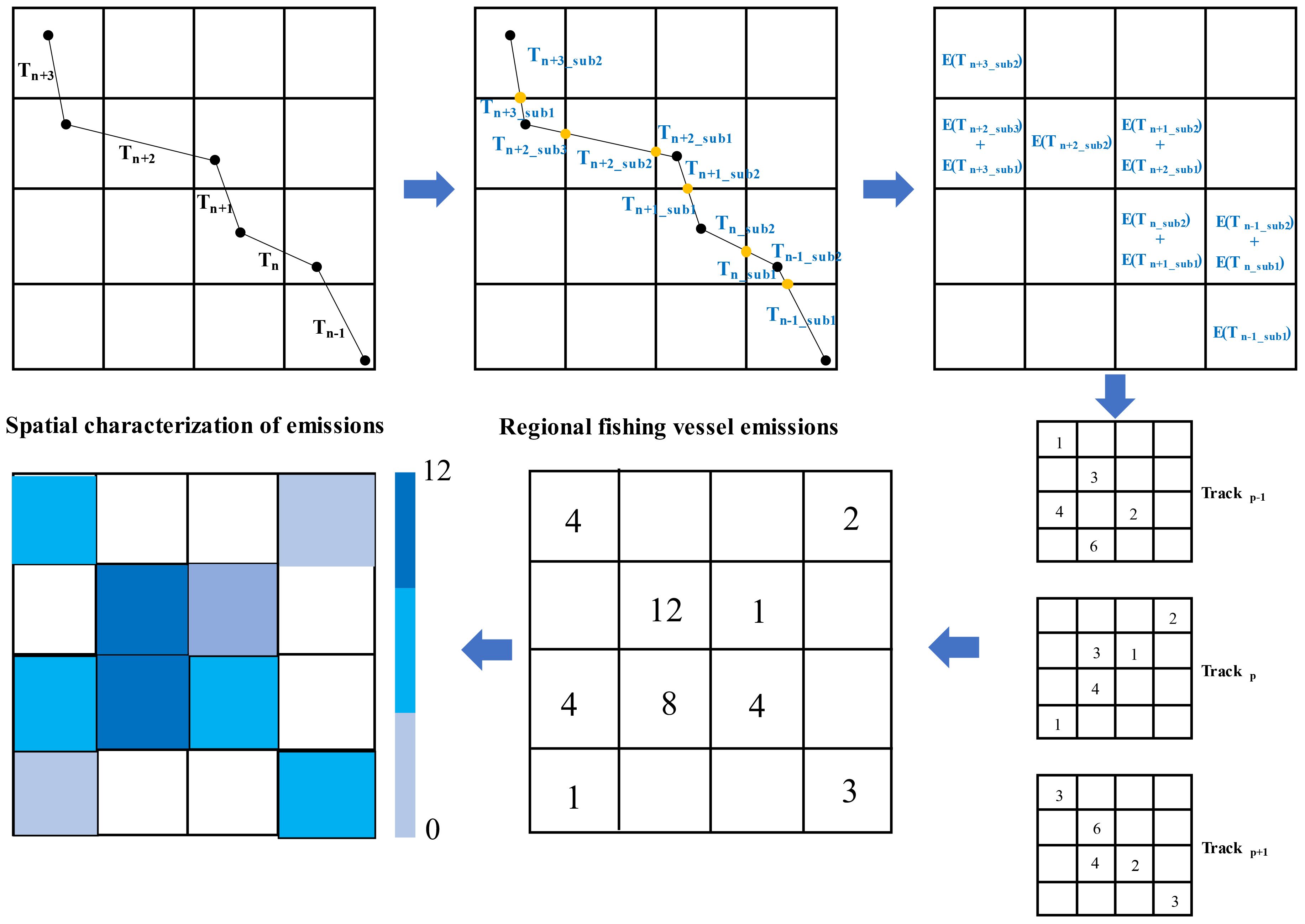
Figure 1 Regional emission statistics for fishing vessels.

4 Methodology

4.1 Estimates of emissions from fishing vessels

This study used a bottom-up activity-based approach as the basic method for estimating vessel emissions. The ‘bottom-up’ approach accurately calculates the trajectory emissions between consecutive positional points, based on a ship’s dynamic data. Furthermore, it can efficiently integrate and count the emission data of all ships. In emissions analysis, the method takes into consideration a ship’s main engine power scale and loading condition, which enables high-precision temporal and spatial analysis of a ship’s emissions. The ‘bottom-up’ approach to estimating emissions from ships can be conducted using Equations 1–4. In this paper, only the emissions from the main engine are taken into account because there is only the main engine and no auxiliary engines or boilers on the fishing vessels involved in the study.

$\begin{array}{ll}{E}_n={\displaystyle {\sum }_{i=1}^{i=I}{E}_{i,n}}& (1)\end{array}$

In Equation (1), E is the total pollutant emission, and n=1, 2, 3, 4, 5, 6, 7, and 8 represent eight different pollutants: CO₂, CO, NO_x, SO₂, PM₁₀, PM_2.5, HC, and CH₄. I is the total number of fishing vessels in the study area on that day.

$\begin{array}{ll}{E}_{i,n}={\displaystyle {\sum }_{j=1}^{j=J}{P}_i\times L{F}_{i,j}\times T_{i,j}\times E{F}_{i,n}\times LL{A}_{i,j}\times {10}^{-6}}& (2)\end{array}$

J is the reporting time of the last VMS message of the fishing vessel. P_i is the main engine power of the fishing vessel. EF_i,n is the emission factor of the vessel, commonly expressed in relation to energy output, i.e. mass of pollutant per unit of energy produced by the engine (g/kWh). LLA_i,j is the low load adjustment factor at time j of the vessel and LF_i,j is the loading of the vessel at time j, which is calculated by Equation (3):

$\begin{array}{ll}L{F}_{i,j}={(\frac{V_{i,j}}{V_{i,max}})}^3& (3)\end{array}$

In Equation (3), V_i,j is the speed of the fishing vessel in the current VMS report information, and V_i,max is the maximum speed of the fishing vessel, which is the highest speed the vessel can achieve at maximum power output, and this is usually determined at the design stage. In this paper, the maximum speed of the fishing vessel is obtained based on the data of the fishing vessel attributes, and there is a difference in the maximum speed depending on the vessel type. T_i,j is the activity time of the fishing vessel, which is calculated by Equation (4):

$\begin{array}{ll}{T}_{i,j}=T_{i,a}-T_{i,a-1}& (4)\end{array}$

In Equation (4), T_i,a and T_i,a-1 represent the current VMS reporting time and the last VMS reporting time, respectively.

4.2 A framework for estimating fishing vessel emissions based on Beidou VMS big data

In this section, a regional fishing vessel emission estimation and statistical framework based on Beidou VMS big data is described in detail.

As shown in Figure 2, the framework consists of three main modules. The first module is used to provide the VMS static data, which includes the attribute information of the fishing vessel, and its purpose is mainly to match the main engine power of the fishing vessel. The second module deals with the processing of dynamic VMS data from fishing vessels and emission estimation. The main tasks of this module consist of processing and trajectory repair of the VMS data, then estimating the emission data sequentially, and spatially assigning and counting the resulting emission data. The third module is mainly responsible for the processing of the meteorological environment, recognizing the wind and current data associated with it (based on the estimated time and region) and is used to correct the speed of the fishing vessel in the second module. Our meteorological environmental data are derived from the Copernicus Marine Database (https://www.copernicus.eu/en) and include data on winds, flows and waves. In particular, the temporal accuracy of wind is 1 hour, and the positional accuracy is 0.125° × 0.125°; the temporal accuracy of flow is 6 hours, and the positional accuracy is 0.083° × 0.083°; and the temporal accuracy of the wave is 3 hours, and the positional accuracy is 0.083° × 0.083°. The specific algorithmic model is shown in Table 1.

Figure 2

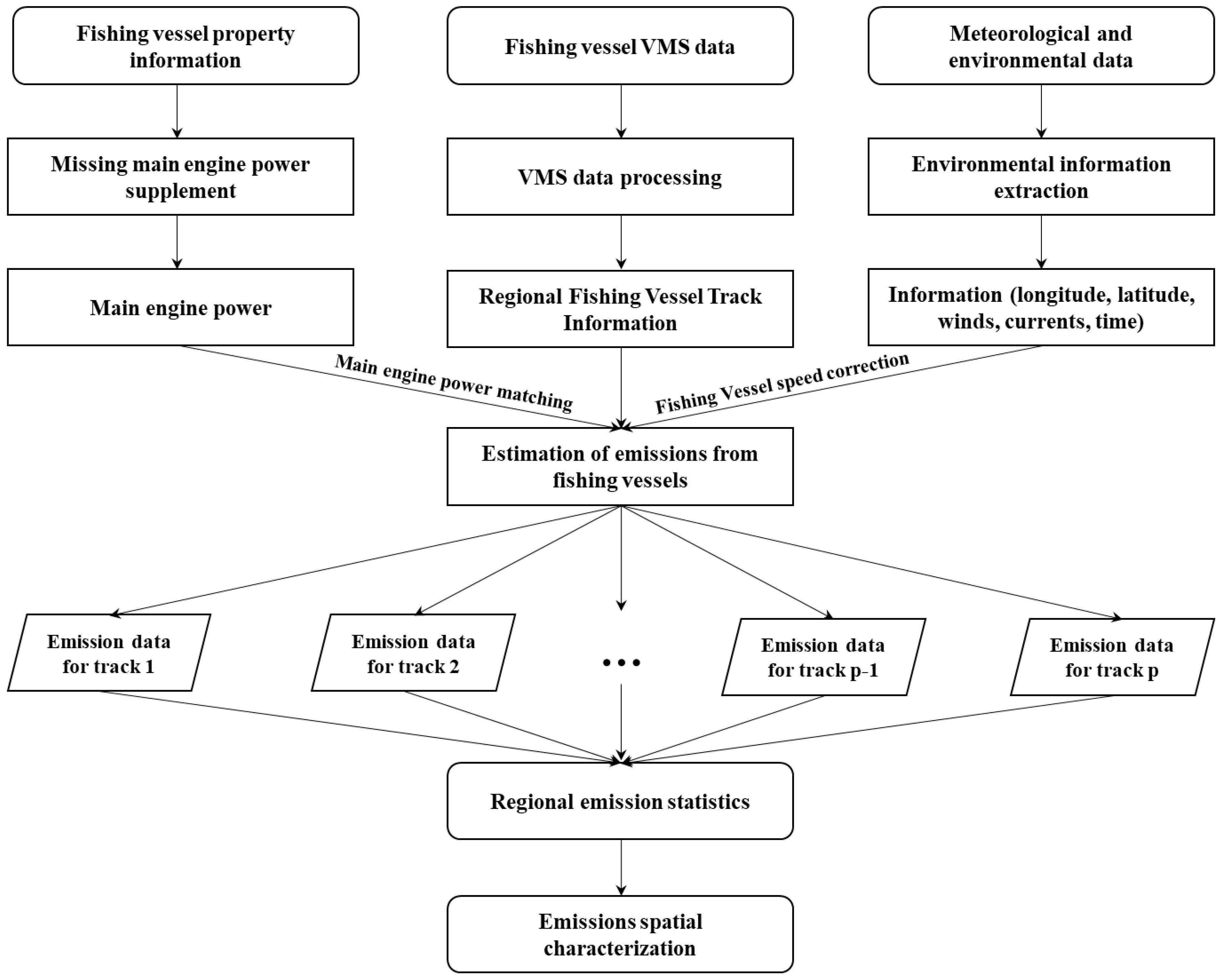
Figure 2 Schematic diagram of the estimation framework of fishing vessel emissions based on big data of Beidou.

Table 1

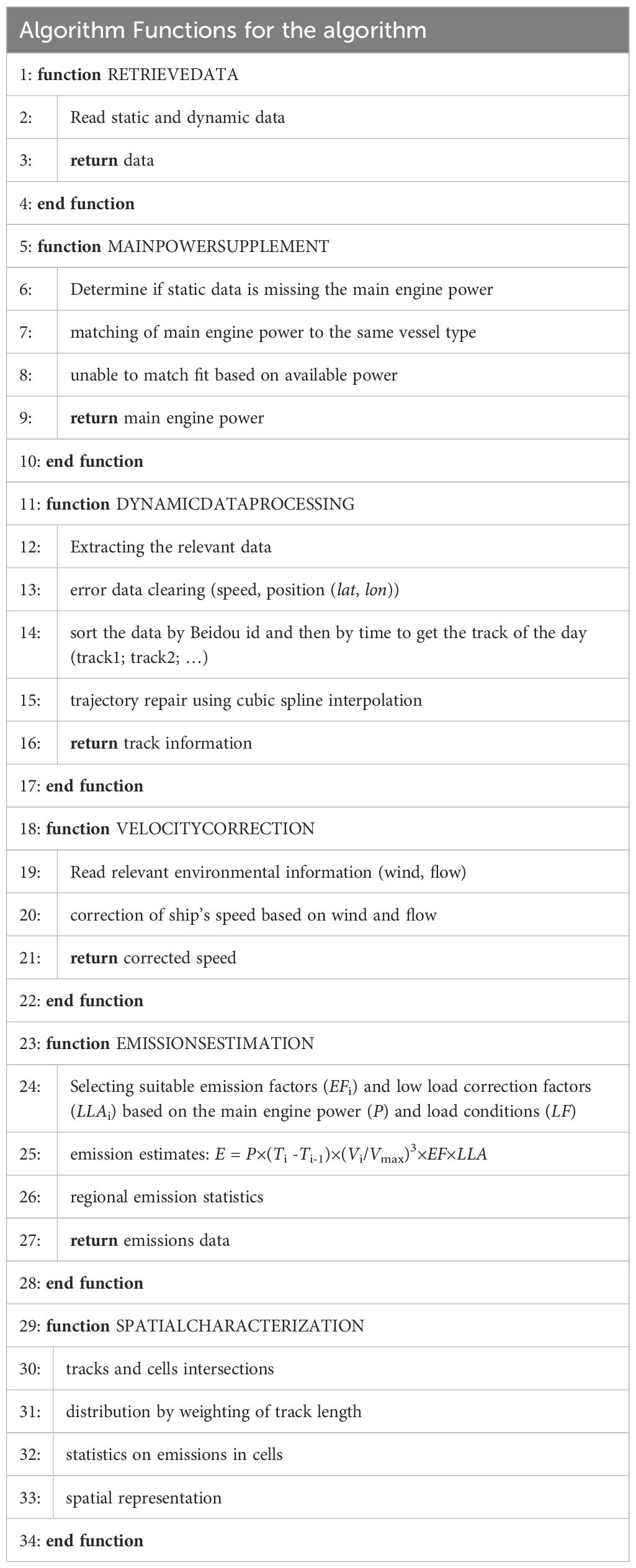
Table 1 Framework for estimating emissions from fishing vessels.

It should be noted that, since the data is stored on a daily basis when a fishing vessel operates continuously at night, it is not possible to estimate the emission of a segment of the trajectory, which may introduce an error. There is a 1-minute time gap between VMS dynamic information broadcasts; to solve this problem, we saved the last trajectory information of the fishing vessels that still had dynamic information after 23:59 every day. Then, based on the Beidou IDs of the fishing vessels, the saved information was matched and merged with the vessels that still had dynamic information before 00:01 the next day, to avoid omission of emissions due to continuous night-time operation of the fishing vessels.

5 Case study

In this section, a framework for estimating emissions from fishing vessels using a bottom-up dynamics approach based on fishing vessel Beidou VMS (vessel monitoring system) big data is applied to investigate the activities of fishing vessels of Zhejiang Province in the East China Sea.

5.1 Study area

The East China Sea is part of the China Sea, one of China’s three marginal seas. It is in the coastal area of five provinces and cities (Jiangsu, Shanghai, Zhejiang, Fujian and Taiwan), and the entire sea lies between latitudes 23˚00’ and 33˚10’ North and longitudes 117˚11’ and 131˚00’ East. The detailed distribution is shown in Figure 3, the waters include 17 major Chinese fishing grounds and the waters of the China-Japan Fishing Vessel Agreement on Provisional Measures, which are abundant in fish resources and have numerous fishing vessels (Chang et al., 2012; Lee et al., 2017).

Figure 3

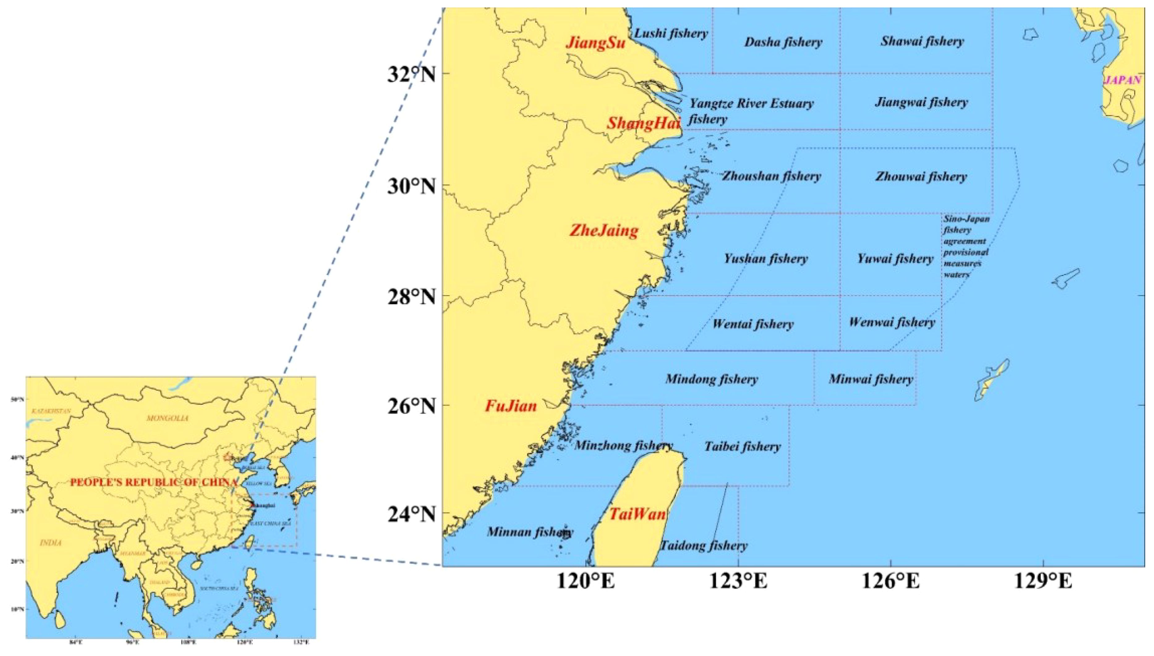
Figure 3 Geographic location of the East China Sea, containing 17 major fishing grounds and the waters of the Sino-Japanese Fisheries Agreement on Temporary Measures.

5.2 Data processing

5.2.1 Area filtering

Our original data cover the East China Sea and Yellow Sea region from 23°N/117°E to 35°05′N/131°E, the data volume of the whole day is about 700 MB. Therefore, to improve the computational efficiency, we filtered out the data outside the study area. The procedure is to check on a record-by-record basis whether the fishing vessels are performing activities in the study area or not. Let lat and lon be the latitude and longitude values in the VMS records, lat and lon should satisfy the Equations 5–10:

$\begin{array}{ll}la{t}_{min}=min(la{t}_{1,min},la{t}_{2,min},\cdots ,la{t}_{N,min})& (5)\end{array}$

$\begin{array}{ll}la{t}_{max}=min(la{t}_{1,max},la{t}_{2,max},\cdots ,la{t}_{N,max})& (6)\end{array}$

$\begin{array}{ll}lo{n}_{min}=min(lo{n}_{1,min},lo{n}_{2,min},\cdots ,lo{n}_{N,min})& (7)\end{array}$

$\begin{array}{ll}lo{n}_{max}=min(lo{n}_{1,max},lo{n}_{2,max},\cdots ,lo{n}_{N,max})& (8)\end{array}$

$\begin{array}{ll}la{t}_{min}<lat<la{t}_{max}& (9)\end{array}$

$\begin{array}{ll}lo{n}_{min}<lon<lo{n}_{max}& (10)\end{array}$

where lat_i,min, lat_i,max, lon_i,min and lon_i,max are the minimum latitude, maximum latitude, minimum longitude and maximum longitude of Leg i (i = 1, 2, ⋯,N), respectively.

5.2.2 Data cleaning

Due to equipment problems, signal transmission, environmental interference etc., VMS data will inevitably have errors and deficiencies, which will not be conducive to the estimation of emissions from fishing vessels. Therefore, pre-processing of VMS data is essential.

In this study, we applied the algorithms of Feng et al. (2022) and Lin et al. (2023) to perform data cleaning, which is based on the mid-division latitude method. Firstly, we calculated the distance between the positions at time t_j and t_j+1 under the unique Beidou ID according to Equation (11):

$\begin{array}{ll}{D}_{i,tj}=\sqrt{{((lo{n}_{i,t_j}-lo{n}_{i,t_{j+1}})cos((la{t}_{i,t_j}+la{t}_{i,t_{j+1}})/2))}^2+{(la{t}_{i,t_j}-la{t}_{i,t_{j+1}})}^2}& (11)\end{array}$

where lat_{i, j} and lon_{i, tj} are separately the latitude and longitude of the fishing vessel with Beidou ID i at the time t_j; lat_{i, tj+1} and lon_{i, tj+1} denote the latitude and longitude at the time t_j+1.

Secondly, the mean μ and variance s of the study area D_i, t_j were obtained according to Equations (12) and (13):

$\begin{array}{ll}\mu =\frac{{\displaystyle {\sum }_{i=1}^{i=I}{\displaystyle {\sum }_{j=1}^{j=J_{i-1}}{D}_{i,t_j}}}}{{\displaystyle {\sum }_{i=1}^{i=I}(J_{i-1})}}& (12)\end{array}$

$\begin{array}{ll}s=\sqrt[2]{\frac{{\displaystyle {\sum }_{i=1}^{i=\text{I}}{\displaystyle {\sum }_{j=1}^{j=J_{\text{i}-1}}{(D_{\text{i},{\text{t}}_{\text{j}}}-\mu )}^2}}}{{\displaystyle {\sum }_{i=1}^{i=I}(J_{\text{i}-1})}}}& (13)\end{array}$

where J_i is the recorded serial number of the fishing vessel with Beidou ID i in the study area; I denotes the total quantity of fishing vessels in the selected area.

Finally, remove the anomalous data. In the case of the VMS data in 2021 9/16, according to our statistics, 8,216,144 distances were obtained, of which 130,982 were outside the interval of μ+3σ. In other words, 98.406% of the distances are less than μ+3σ. According to Feng et al. (2022), points falling outside μ + 3σ are usually anomalous. Therefore, we removed these data. Figure 4 shows the trajectory maps of the original data and the cleaned data on 16 September 2021.

Figure 4

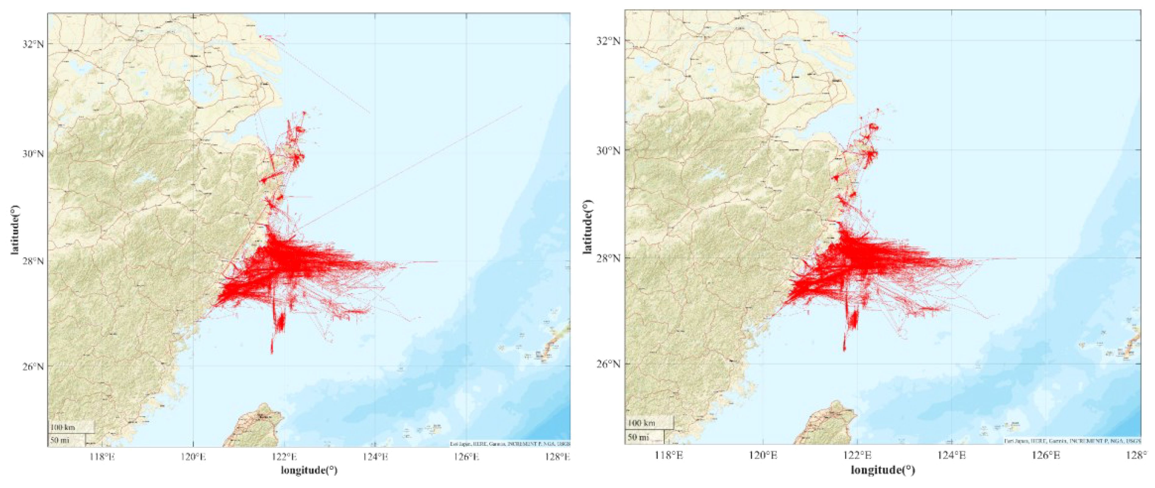
Figure 4 VMS trajectory plot in the East China Sea for fishing vessels on 16 September 2021, original trajectory (left) and trajectory plot after data cleaning (right).

5.2.3 Trajectory repairing

After clearing the anomalous data, it will lead to some trajectory points of the fishing vessel missing, and it has been mentioned before that the minimum time accuracy of our VMS data is 3min, in our actual research, we found that the time accuracy is different for different fishing vessels, including 3, 6, 10, 12min, etc. So we repair the trajectory of the two trajectory points whose time interval exceeds the temporal accuracy of the vessel based on the method of Hintzen et al. (2010) and Huang et al. (2020) to make them satisfy the time accuracy as close to temporal accuracy as possible, to reduce the emission error due to the missing trajectory. Firstly, we will determine the number of insertion points according to Equation (14):

$\begin{array}{ll}k=\frac{\Delta t_i-T{H}_i}{T{H}_i}-1& (14)\end{array}$

where k = (1, 2, 3,…, n) is the number of trajectory points to be inserted; Δt_i is the time interval of the ship’s trajectory; the time interval with the highest number of occurrences is defined as the time threshold TH_i; if Δt_i ≥ 2TH_i, we mark that the trajectory is missing between these two points and needs to be repaired according to Equation (15) and Equation (16).

$\begin{array}{ll}la{t}_{i,k}=la{t}_i+v_i\times sin\theta \times T{H}_i\times W& (15)\end{array}$

$\begin{array}{ll}lo{n}_{i,k}=lo{n}_i+y_i\times cos\theta \times T{H}_i\times (1-W)& (16)\end{array}$

where θ is the spatial angular difference between the two trajectory points to be interpolated, calculated according to Equation (17); and W is the weight factor, which can be assigned to the time interval between the interpolated point and the first interpolated point.

$\begin{array}{ll}\theta =arccos[sinla{t}_i*sinla{t}_{i+1}+coslo{n}_i*coslo{n}_{i+1}*cos(lo{n}_i-lo{n}_{i+1})]\frac{180}{\pi }& (17)\end{array}$

According to this approach, 183,247 track points are added for the data of September 16, 2021.

5.2.4 Main engine power fitting

In the study, we found that Chinese fishing vessels have a strong regularity in main engine power, length, and width compared with other types of vessels. As shown in Table 2, ‘NINGYU’, ‘ZHEFENGYU’ and ‘ZHENINGYU’ have the same main engine power with the same length and width (Only a few examples of fishing vessels), which is mainly due to the standardization of the design and construction of Chinese fishing vessels (they are all manufactured by the same shipyard). When a vessel lacks main engine power, we matched the main engine power of the fishing vessel with the static information in the VMS, i.e. vessel ID, vessel name, and length and width of the vessel. This is an advantage for Chinese fishing vessels, over other large ocean-going vessels.

Table 2

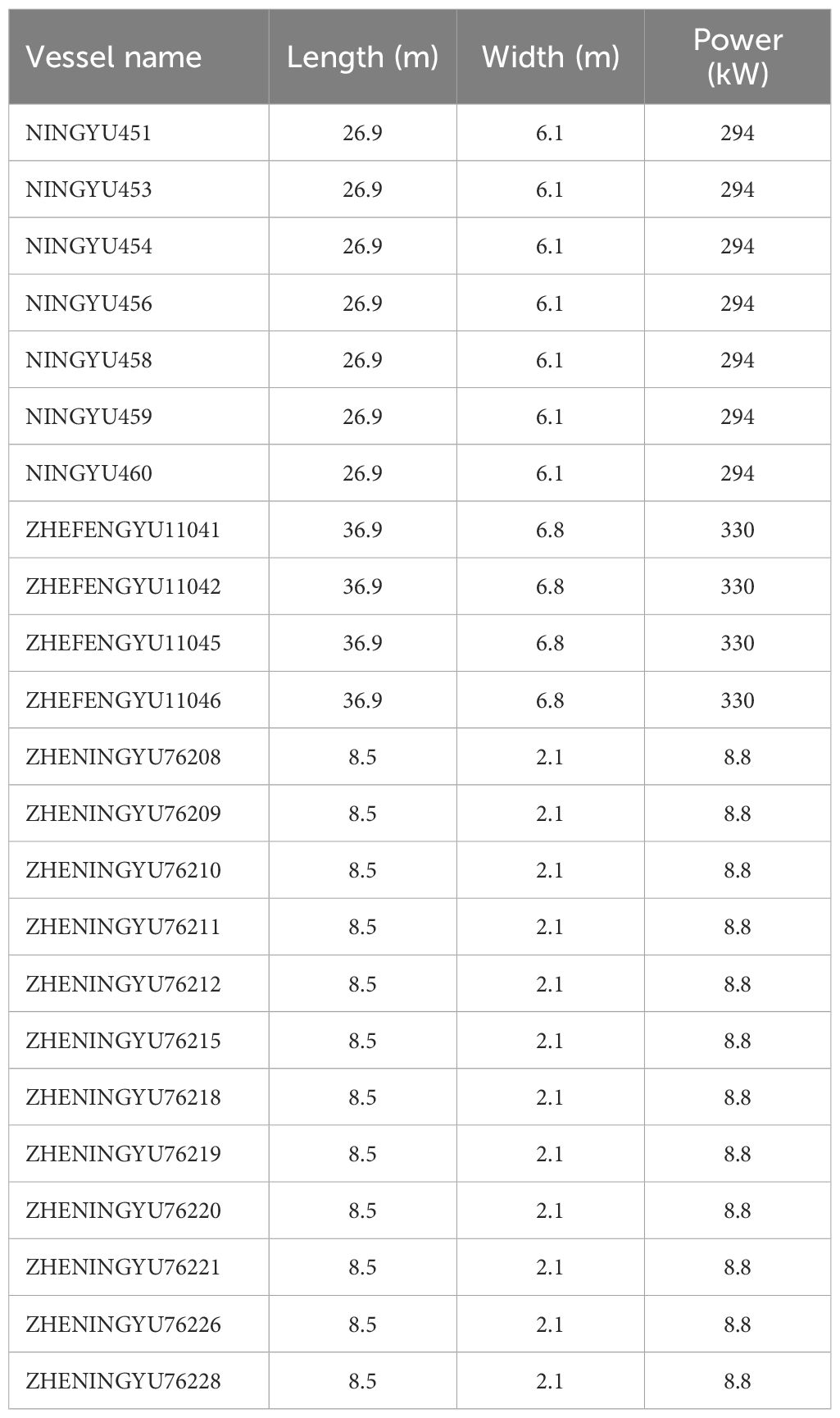
Table 2 Length, width, and main engine power of some fishing vessels.

In cases where the main engine power of some fishing vessels was missing and could not be matched with the main engine power of existing vessels, we fitted them to the data of existing vessels. The fitting results are shown in Figure 5, which shows that the best result is obtained by fitting the ship’s main engine power to the product of the ship’s length and width. In this sense, our results are following Huang et al. (2020), in which the R² is 0.9052. Figure 6 shows the fitted curves and the corresponding error distributions.

Figure 5

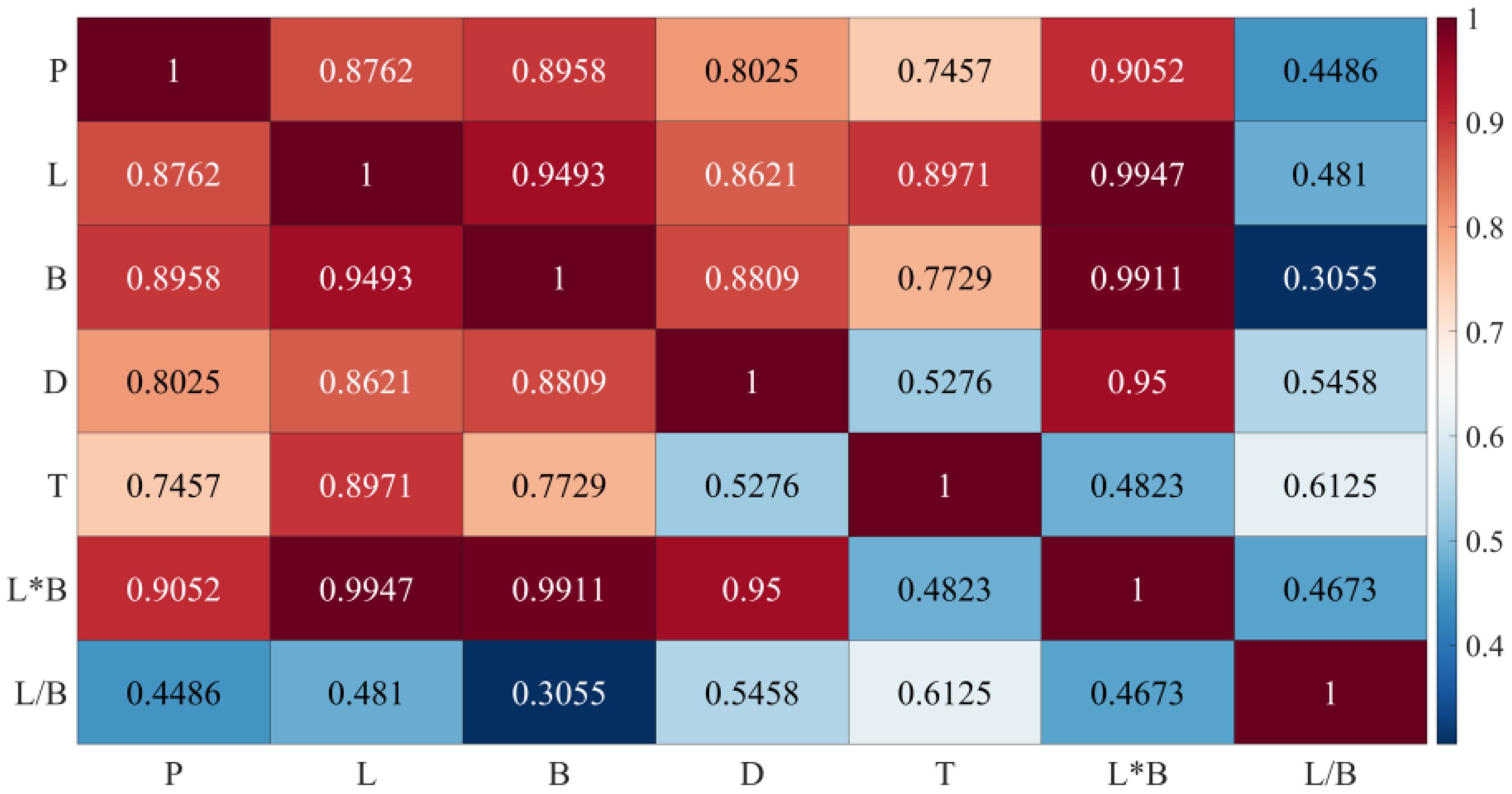
Figure 5 Heat map of correlation coefficients between main engine power and vessel attributes (P - main engine power, L - length of vessel, B - breadth of vessel, D - depth of vessel, T - tonnage of vessel).

Figure 6

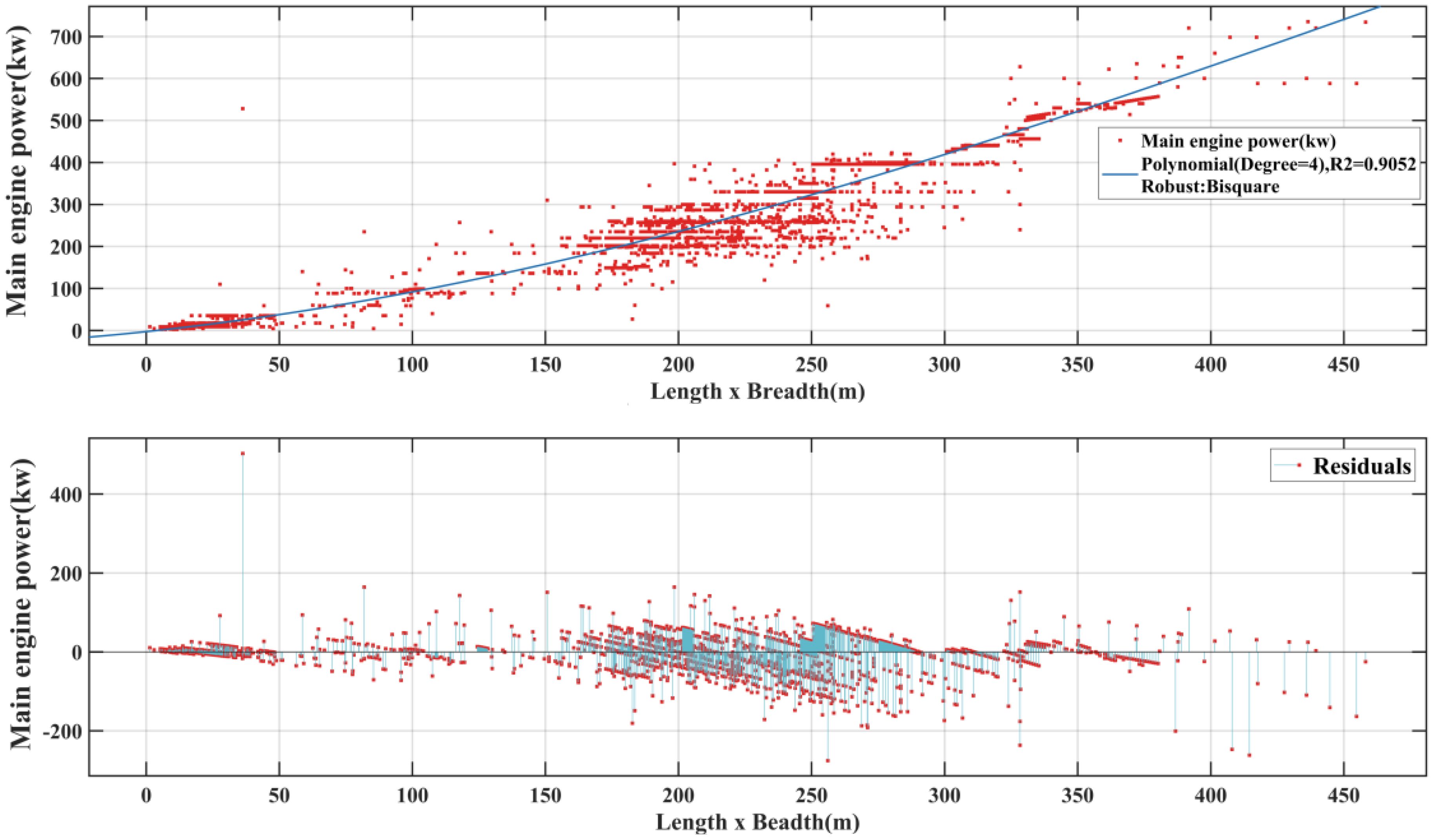
Figure 6 The fitted curves and fitted variance distributions for the main engine power and length × width.

5.2.5 Emission factors

When estimating ship emissions using the bottom-up dynamic approach, the ship emission factor is a major factor affecting the accuracy of the estimation (Zhang et al., 2018; Grigoriadis et al., 2021). Therefore, it is crucial to use accurate and reliable emission factors for the establishment of emission inventories. Grigoriadis et al. (2021) developed a new set of ship emission factors based on the existing factors, using a review and meta-analysis-based approach that allowed for the selection of appropriate ship emission factors based on engine and fuel type. Therefore, the emission factors for CO₂, CO, NO_x, SO₂, HC, PM₁₀ and PM_2.5 in this research adopt the results of Grigoriadis et al. (2021), and the emission factor for CH₄ follows the recommended data by IMO (https://www.imo.org/en/). The framework proposed in this paper allows for the selection of appropriate vessel emission factors based on the type of fishing vessel main engine. The specified emission factors are listed in Table 3.

Table 3

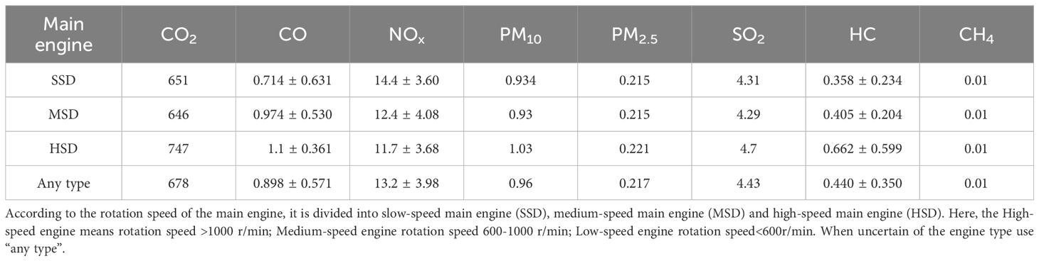
Table 3 The emission factors for each pollutant (unit: g/kWh).

5.3 Results

In total, our VMS dataset recorded 2.825 billion VMS messages, with a daily average of 7.8472 million reports. Depending on the type of operation, there are more than 10 types of fishing vessels, including gillnets, purse seines, cast nets, trawlers, fishing gears, fishing transportation, cage pots, rakes and spikes, fishing gears, etc. The most common types of these operations are trawling, gillnetting, purse seining, fishing gear, fishing tackle, and fishing transportation.

5.3.1 Fishing vessel statistics

Based on our VMS data, as shown in Figure 7, 18,487 Zhejiang fishing vessels were found in the East China Sea from June 1, 2021, to May 31, 2022, accounting for 5.18% of all (marine and non-marine) motorized fishing vessels (357,000) in China in 2021. This gives an average of 14,688.69 per day, of which the maximum number can be up to 17,878 in one day. The fishing intensity in the East China Sea during the peak period was extremely high. The gross power of fishing vessels was 2.692 million kW, accounting for 14.6% of the total power of all motorized fishing vessels in China (18.452 million kW) in 2021, while the average power of the main engine of fishing vessels reached 149.88 kW. The average main engine power of a single vessel in Zhejiang fishing vessels is a bit larger than usual.

Figure 7

Figure 7 Quantity of fishing vessels from 1^st June 2021 to 31^st May 2022.

5.3.2 Emission inventory

We estimated that the total emissions of CO₂, CO, NO_x, PM₁₀, PM_2.5, SO₂, HC, and CH₄ from fishing vessels in Zhejiang Province in the East China Sea, during the period June 1, 2021 to May 31, 2022, were 2.8×10⁵ t, 1.3×10³ t, 6.9×10³ t, 632.03 t, 577.8 t, 1.67×10³ t, 359.9 t, and 28.88 t, respectively. The highest emissions and emission intensity occurred in October 2021, followed by September, and then December. Geographically, these emissions were mainly concentrated in the fisheries at the Yangtze River estuary Fishery, Zhoushan Fishery, Yushan Tishery, Wentai Fishery, Zhouwai Fishery, and Jiangwai Fishery, along the coasts of Shanghai and Zhejiang. Table 4 presents the specific emission inventories. The emissions and emission intensities of each pollutant for each month are reported in Figure 8. The distributions of each pollutant emission in the East China Sea are shown in Figure 9.

Table 4

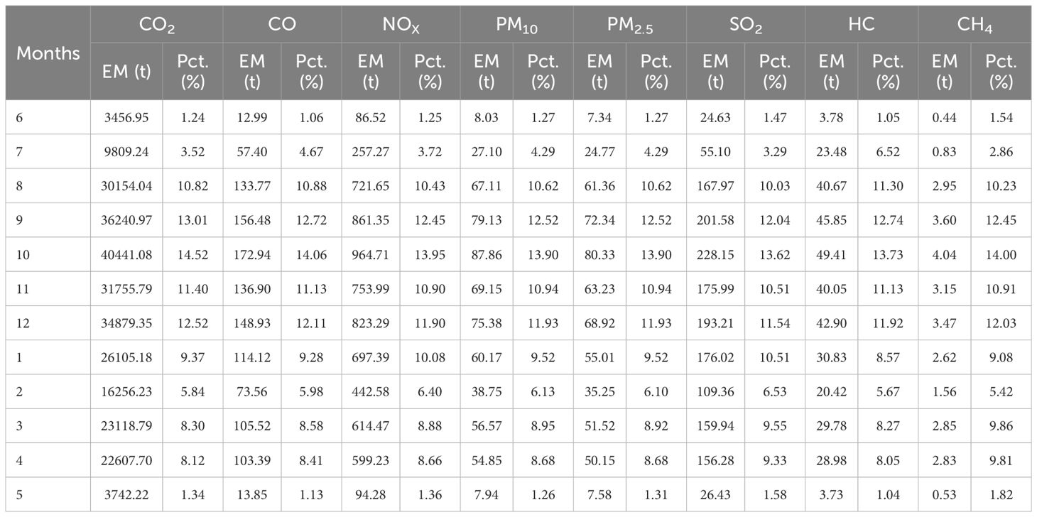
Table 4 Emission Inventory of Fishing Vessels in East China Sea Zhejiang Province, June 2021-May 2022.

Figure 8

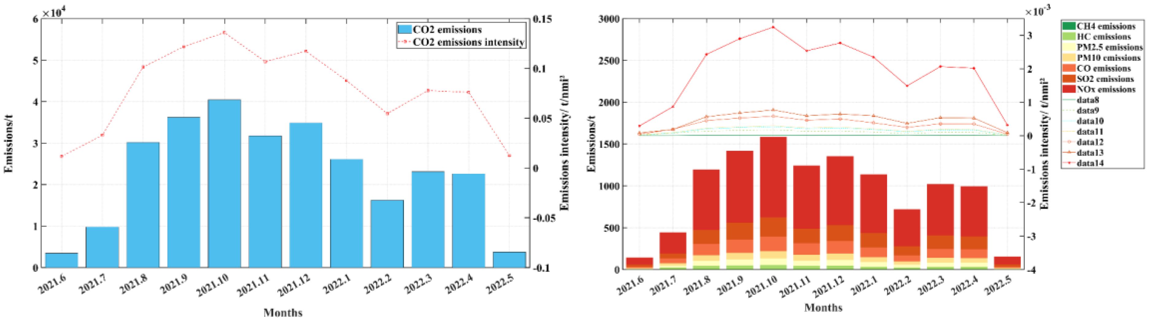
Figure 8 Emissions and emission intensity of pollutants by month, from June 2021 to May 2022 (CO₂ on the left and other pollutants on the right).

Figure 9

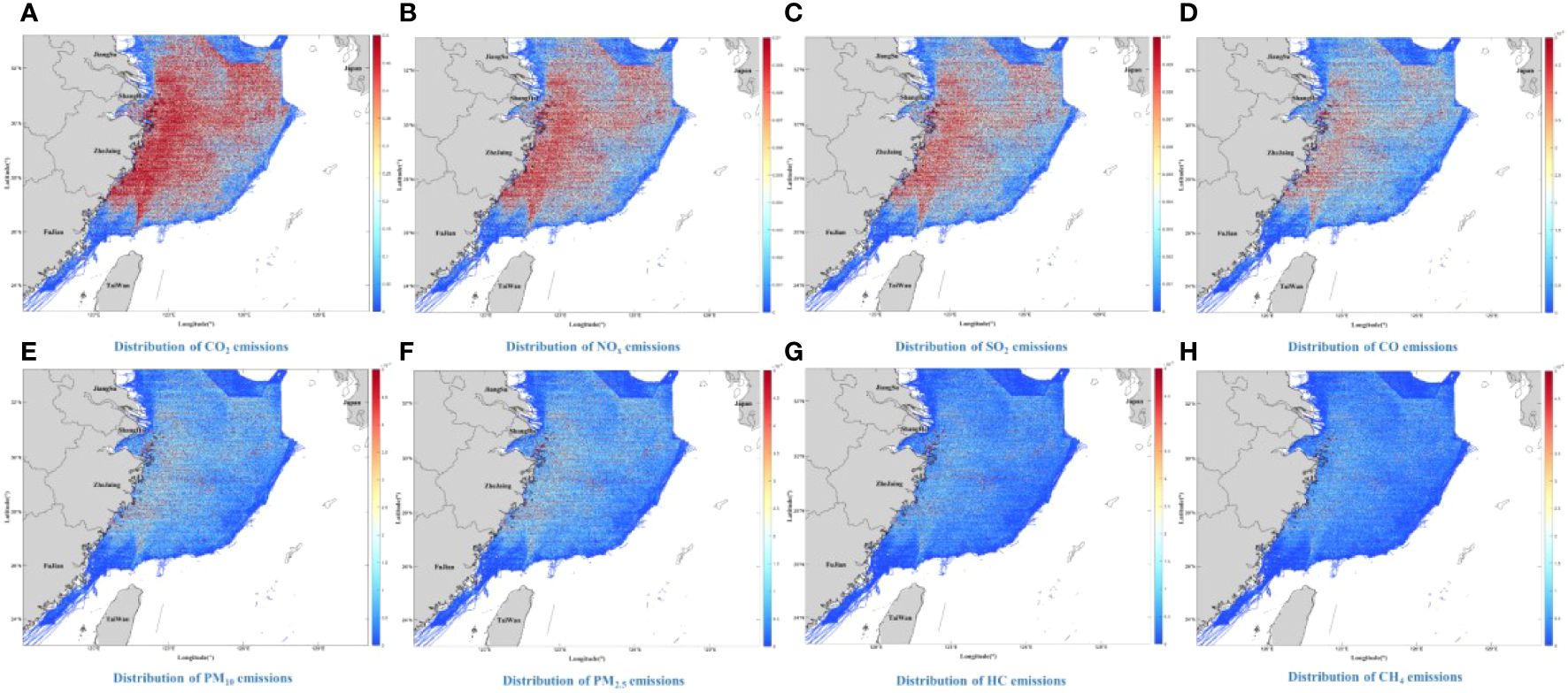
Figure 9 Emission distribution by pollutant over the study period. (A) for CO₂, (B) for NO_x, (C) for SO₂, (D) for CO, (E) for PM₁₀, (F) for PM_2.5, (G) for HC and (H) for CH₄.

5.3.3 Emissions over time

The temporal variation of emissions of each pollutant emitted by fishing vessels in Zhejiang Province in the East China Sea is shown in Figure 10. It can be seen that in June and July, the emissions of each pollutant were generally low. However, emissions increased significantly from August 1 and rose to higher levels after September 16. Later, the emissions fluctuated but remained at a high level. After May 1, 2022, emissions dropped to lower levels, roughly in line with the emissions of June 2021.

Figure 10

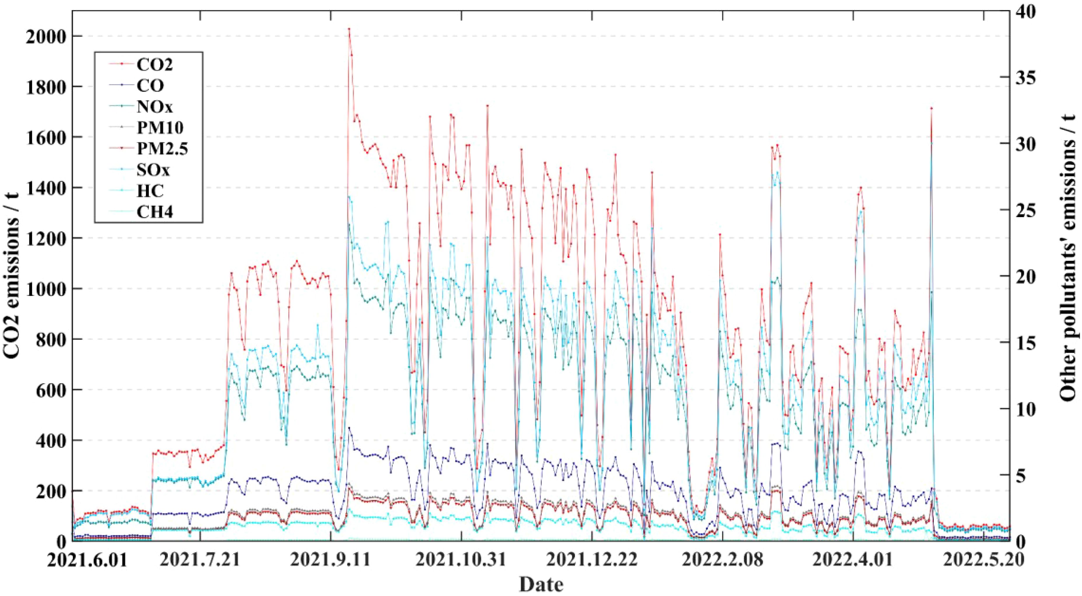
Figure 10 Emissions of pollutants over time (Note: CO₂ emissions on the left axis and emissions of other pollutants on the right axis).

6 Discussion

6.1 Emissions

According to the China Mobile Source Environmental Management Annual Report 2022(https://www.mee.gov.cn/hjzl/sthjzk/ydyhjgl/202212/W020221207387013521948.pdf), in 2021 Chinese non-road mobile sources emitted 168,000 tonnes of SO₂, 429,000 tonnes of HC, 4,789,000 tonnes of NO_x, and 234,000 tonnes of PM, respectively. Based on our estimation, the SO₂, HC, NO_x, and PM emitted from fishing vessels in Zhejiang Province in the East China Sea, during the year from June 2021 to May 2022, accounted for 1.000%, 0.080%, 0.144%, and 0.520% of Chinese non-road mobile source emissions in 2021 (PM₁₀+PM_2.5), respectively. In addition, according to the latest carbon emissions data from the China Carbon Accounting Database (https://www.ceads.net.cn/), Chinese mobile sources emitted a total of 0.83 billion tonnes of carbon dioxide in 2019, while our estimated carbon emissions from Zhejiang fishing vessels in the East China Sea fishing grounds accounted for 0.34% of all mobile source carbon emissions. Chen et al. (2022) measured the carbon emissions from marine fisheries in the Northern Marine Economic Circle (NMEC), which represents the development of Chinese marine fisheries, for the years 2006-2019. The largest province in northern China, in terms of fisheries emissions, is Shandong Province which, according to their results, has emitted more than 20,000 tonnes of carbon emissions from fishing vessels, annually, in recent years. According to our estimated results, the annual carbon emissions from fishing vessels in Zhejiang Province are probably as much as ten times higher than those in Shandong Province. It is unexpected that the emission from fishing vessels in Zhejiang Province, which is in the East China Sea alone, is so high, which shows that the emissions from fishing vessels should not be neglected.

6.2 Impact of fishing moratoriums on emissions

The fluctuation of changes in emissions of each pollutant from fishing vessels in June, July, August, September 2021, and May 2022 is probably affected by the seasonal fishing moratorium system. The seasonal fishing moratorium system is a policy which was approved by the State Council of China in 1995, aimed at protecting fishery resources (including fish, shrimp, and crabs) in the Yellow Sea, the East China Sea, and (later) the South China Sea, under China’s jurisdiction, north of latitude 12˚ N (Samy-Kamal et al., 2015).

The specific fishing moratorium system in the East China Sea in 2021 was implemented from noon on May 1 to 12:00 on August 16 in the sea area between 23˚and 26˚30’ N. In contrast, the sea area between 26˚30’ N and 33˚10’ N was prohibited from noon on May 1 to 12:00 a.m. on August 1, for trawlers, cage pots, gillnets, and light seines; for other types of fishing vessels, fishing activities were prohibited until noon on September 16th. All types of operating vessels were restricted by the moratorium, except for fishing gear vessels. The moratorium regime in 2022 was the same as in 2021. This information is derived from a notice by the Fisheries and Fishing Administration of the Ministry of Agriculture and Rural Affairs of the People’s Republic of China (http://english.moa.gov.cn/).

It should be noted that the overall emissions from fishing vessels increased in July 2021, compared to June 2021. Two main reasons could have led to this phenomenon. Firstly, July is the peak season for recreational sea fishing tourism during the summer months, which results in a higher frequency of activities by fishing gear vessels. Secondly, after the two-month fishing ban in May and June, it is possible that some fishing vessels were engaged in illegal fishing activities during the moratorium. This may explain the slight increase in the overall level of emissions from fishing vessels in July.

6.3 Impact of the meteorological environment on emissions

As shown in Figure 10, there were obvious fluctuations in the emissions of fishing vessels in the East China Sea around some dates after September 16th. We hypothesize that this fluctuation may be affected by severe weather events, such as typhoons, cold wave gales, and high waves. To analyze this phenomenon more scientifically, we conducted a statistical analysis of the severe weather (typhoons and cold wave winds) that affected the East China Sea during the period from June 1, 2021, to May 31, 2022. The specific typhoon dates can be found in Table 5, while the cold wave wind data can be found in Table 6. We found that the timing of the effects of these severe weather events and the timing of the fluctuations in fishing vessel emissions roughly coincided. The fishing vessels sailed back to port at high speeds to avoid the winds before the severe weather arrived, and this led to a small increase in emissions. In contrast, emissions were reduced significantly when fishing vessels ceased operation during sheltering periods in ports. After the bad weather was over, fishing vessels left the port to operate centrally, which again led to a sharp increase in emissions. The lower emissions from fishing vessels during the period from the end of January 2022 to February 8, 2022, are mainly due to the Chinese Lunar New Year, when most of the fishing vessel operators take their annual leave to go home for the New Year, resulting in a significant reduction in emissions from fishing vessels. After February 8, with the end of the Lunar New Year, fishing vessels resumed normal operations and emissions returned to normal levels.

Table 5

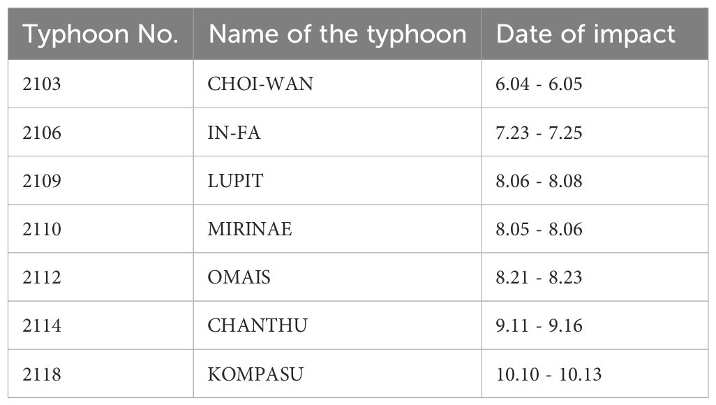
Table 5 Typhoons affecting the East China Sea, June-December 2021.

Table 6

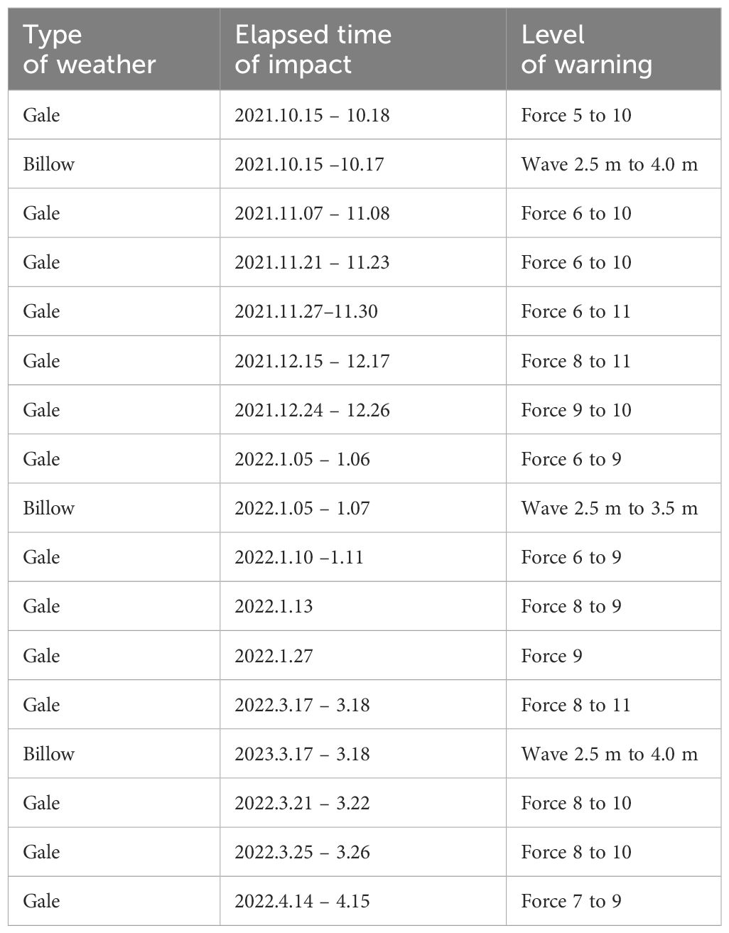
Table 6 Cold waves affecting the East China Sea from June 2021 to May 2022.

In addition, during the lunar cycle, a decrease in emissions was observed compared to other periods. It is hypothesized that this may be due to a reduction in fishing activity by fishing gear with lights during the lunar cycle, which may have contributed to this phenomenon.

Based on the data in Table 4; Figure 10, it is obvious that compared with the autumn and winter seasons (September 2021 to February 2022), the CO₂ emissions from fishing vessels in the East China Sea are generally lower in the spring and summer seasons. More specifically, the distribution of CO₂ emissions in different months is shown in Figure 11. The overall emissions in the autumn and winter seasons are higher, while the emissions in February are relatively lower, mainly due to the influence of the Chinese New Year holiday. We hypothesize that this difference is mainly influenced by the meteorological environment.

Figure 11

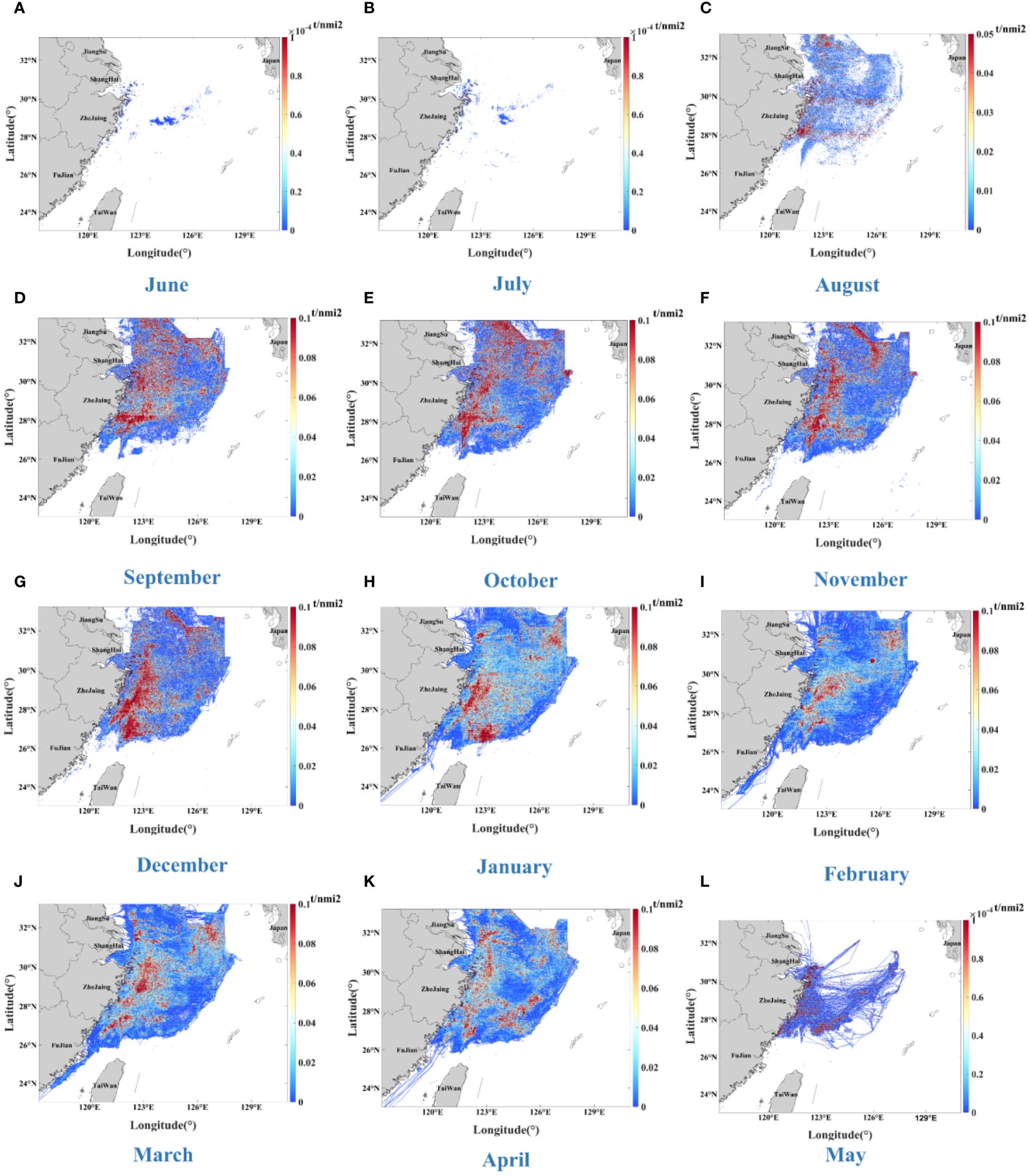
Figure 11 Distribution of CO₂ emissions from fishing vessels in the East China Sea from June 2021 to May 2022 (unit: t/km²). (A) in June 2021, (B) in July 2021, (C) in August 2021, (D) in September 2021, (E) in October 2021, (F) in November 2021, (G) in December 2021, (H) in January 2022, (I) in February 2022, (J) in March 2022, (K) in April 2022 and (L) in May 2022.

To further explore the relationship between fishing vessel emissions and the meteorological environment, we statistically analyzed the wind speed, current speed, and wave height in the East China Sea during the study period. Results show that in spring 2022, wind speed, current speed and wave height in the East China Sea are at a low level compared to other times of the year (according to the heat map shown in Figures 12–23). This means that there are better sea conditions in the spring and fishing boats do not need to use a lot of power to maintain their speed, thus reducing emissions. On the contrary, in the case of a poor sea surface due to meteorological conditions, fishing vessels need to consume more power to maintain their fishing speed to overcome the sea surface conditions, leading to an increase in emissions.

Figure 12

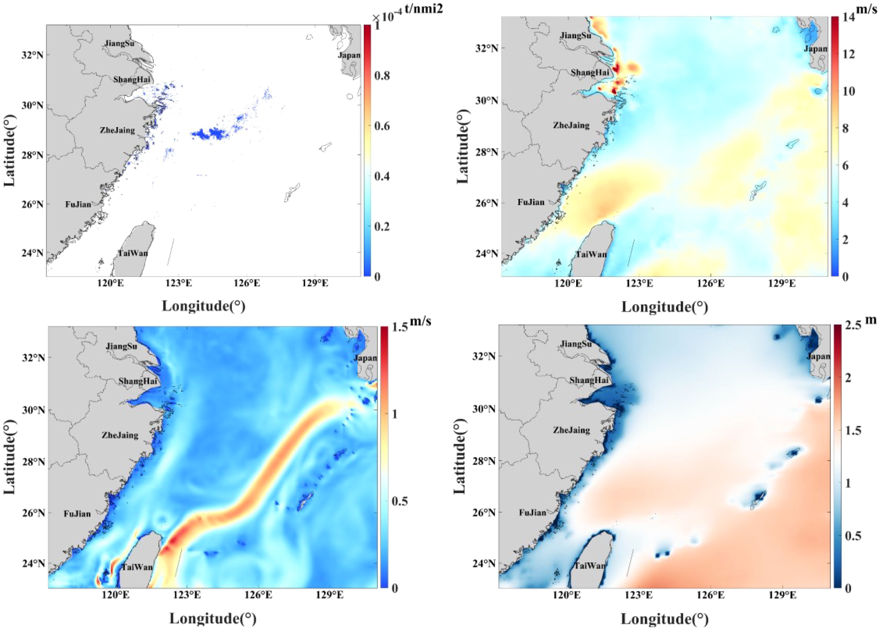
Figure 12 Schematic diagram of CO₂ emissions, wind velocity, flow velocity and wave height in June 2021 (from left to right and top to bottom, the distribution of CO₂ emissions from fishing vessels, wind velocity, flow velocity and wave height, respectively, which are the same as in Figures 13–23).

Figure 13

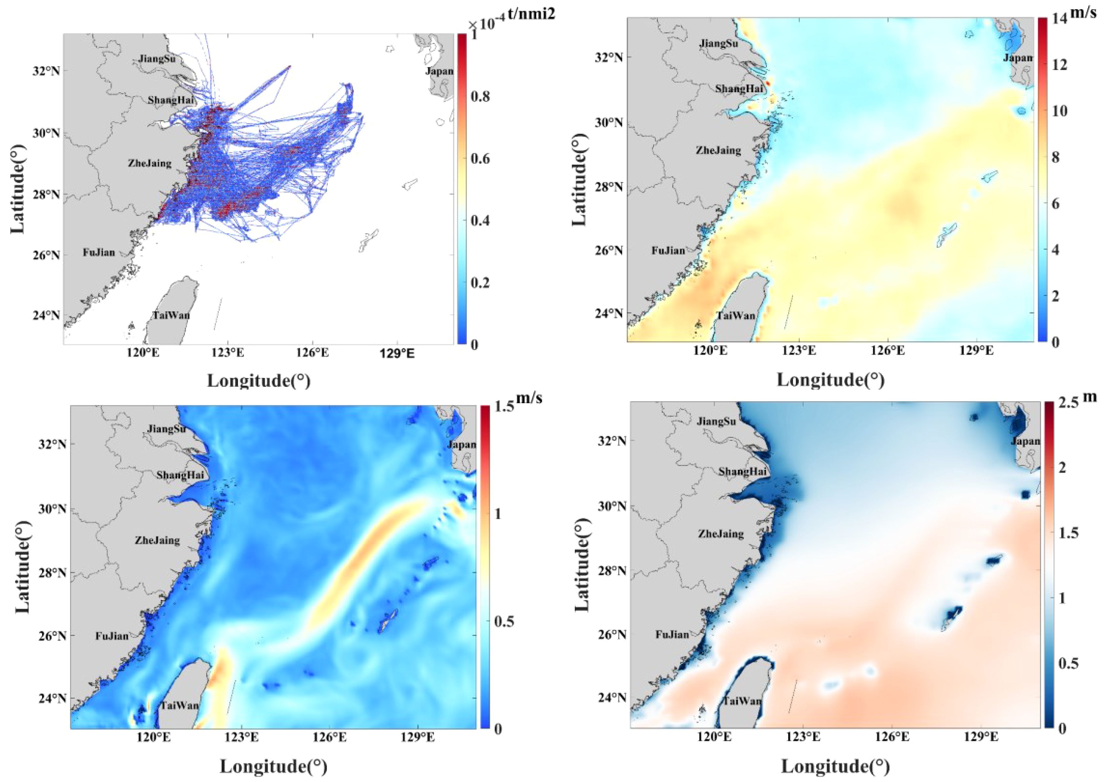
Figure 13 Schematic diagram of CO₂ emissions, wind velocity, flow velocity and wave height in May 2022.

Figure 14

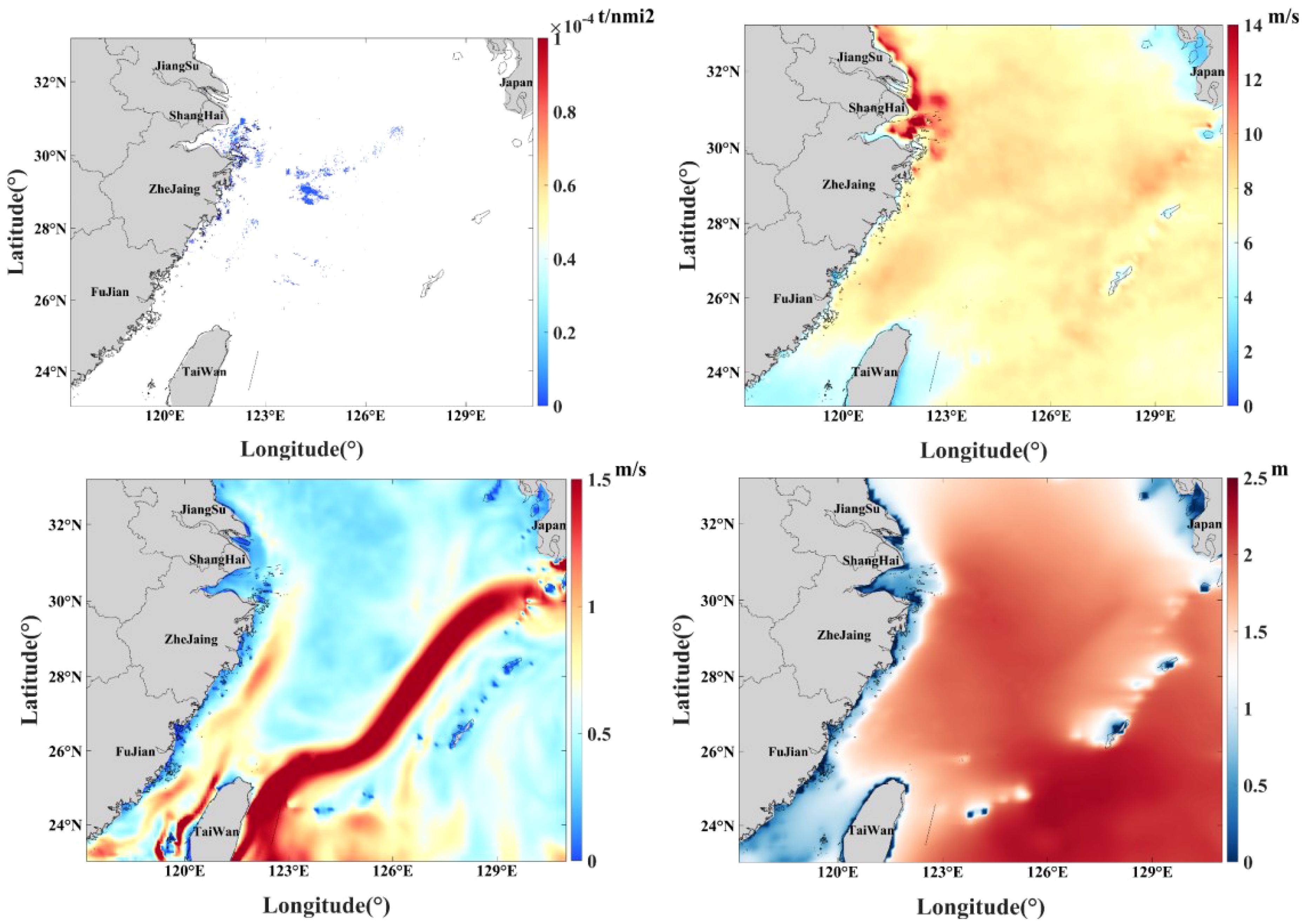
Figure 14 Schematic diagram of CO₂ emissions, wind velocity, flow velocity and wave height in July 2021.

Figure 15

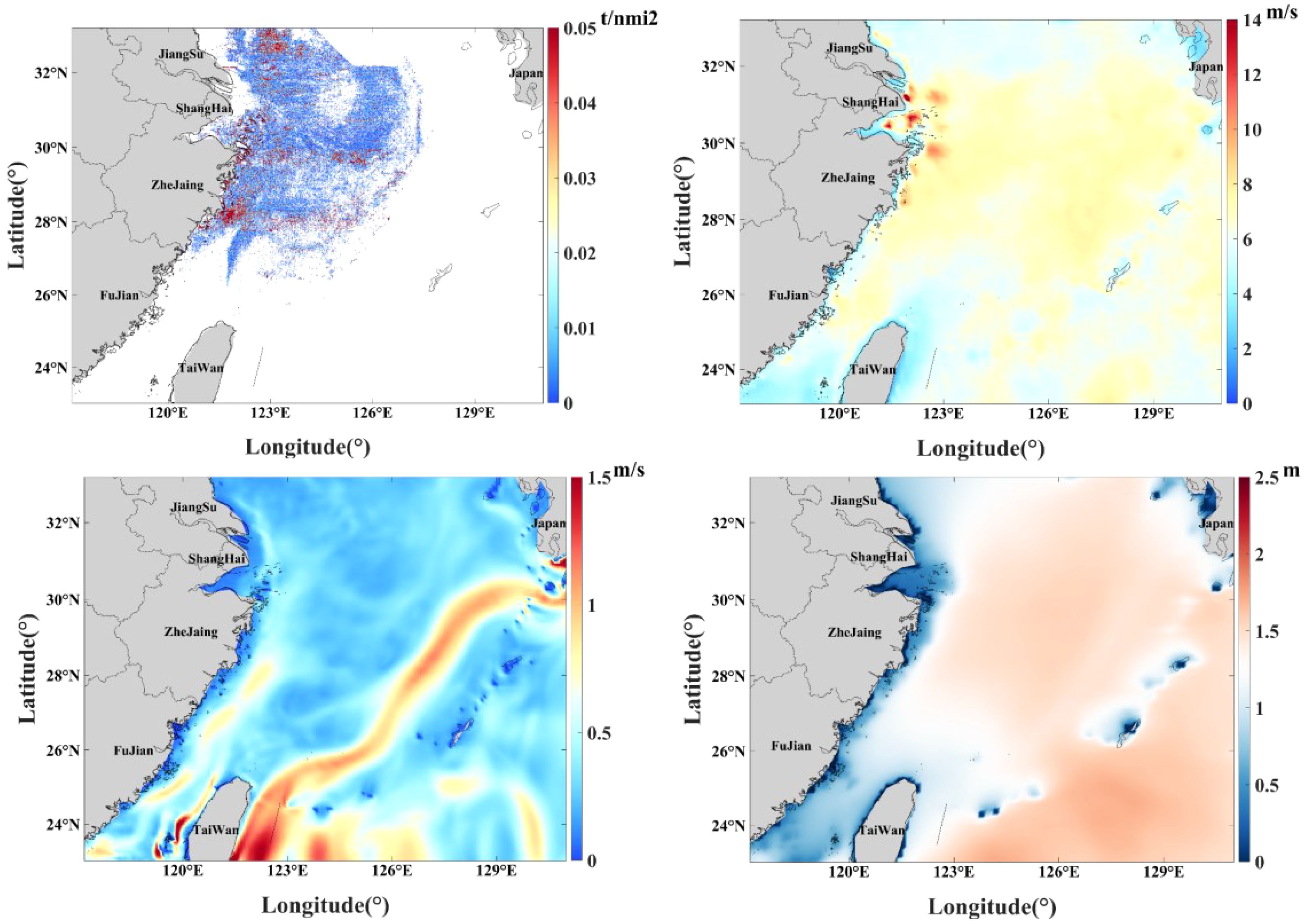
Figure 15 Schematic diagram of CO₂ emissions, wind velocity, flow velocity and wave height in August 2021.

Figure 16

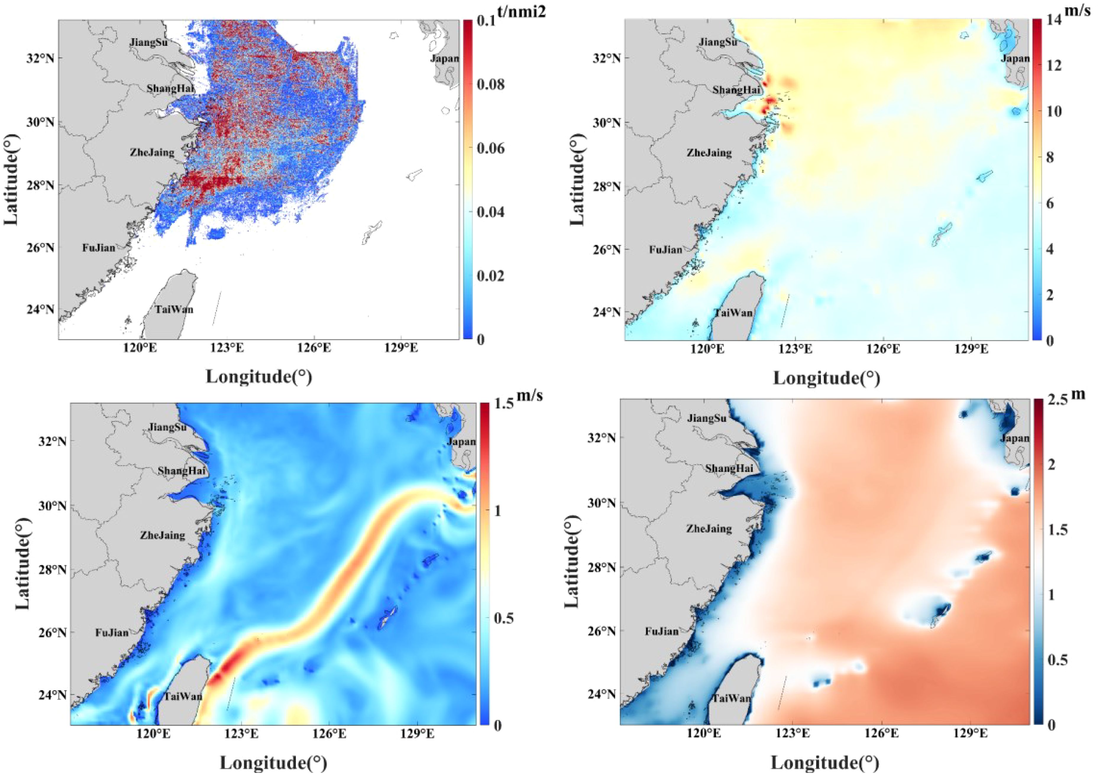
Figure 16 Schematic diagram of CO₂ emissions, wind velocity, flow velocity and wave height in September 2021.

Figure 17

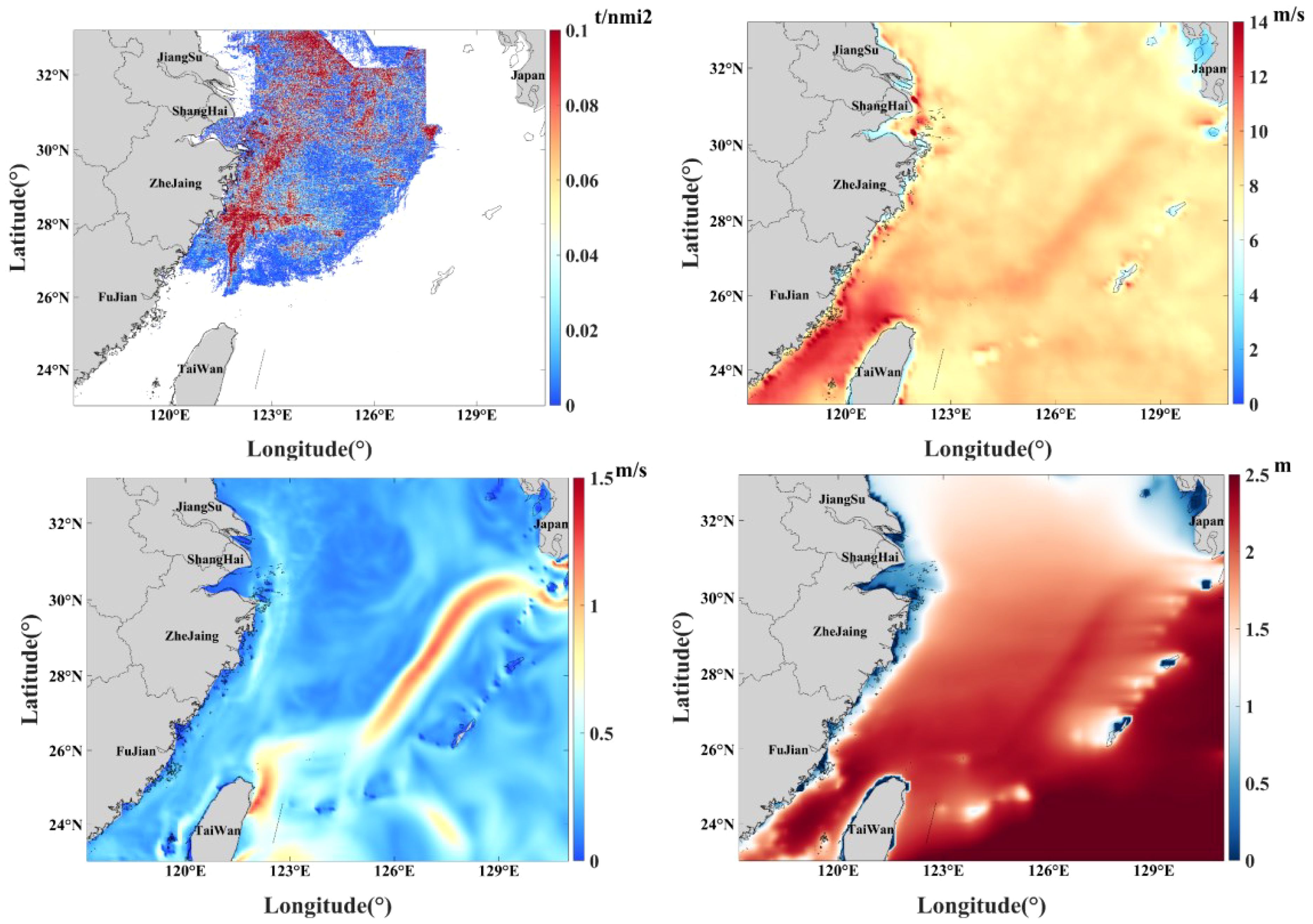
Figure 17 Schematic diagram of CO₂ emissions, wind velocity, flow velocity and wave height in October 2021.

Figure 18

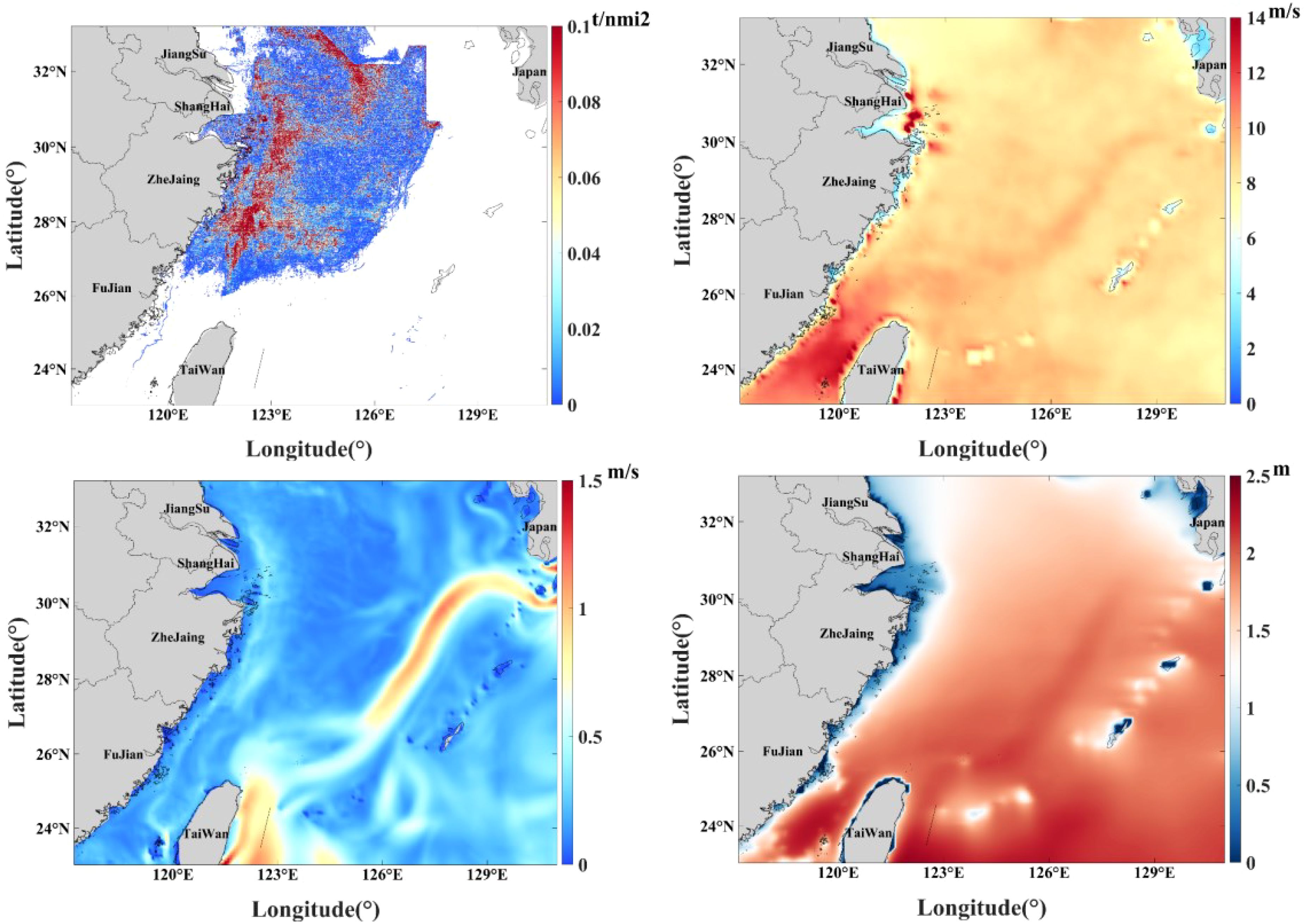
Figure 18 Schematic diagram of CO₂ emissions, wind velocity, flow velocity and wave height in November 2021.

Figure 19

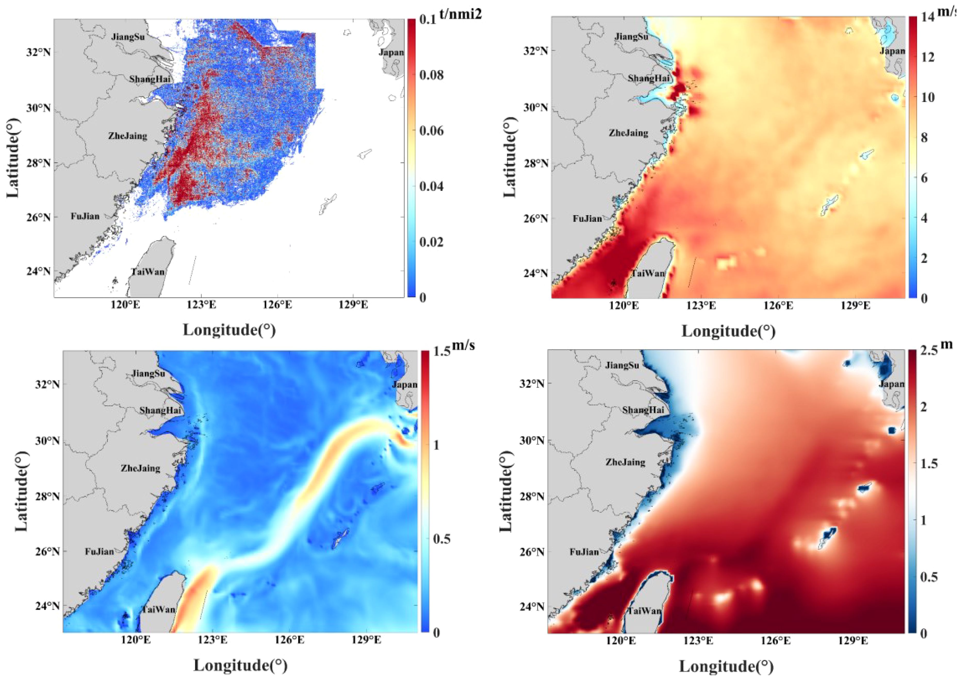
Figure 19 Schematic diagram of CO₂ emissions, wind velocity, flow velocity and wave height in December 2021.

Figure 20

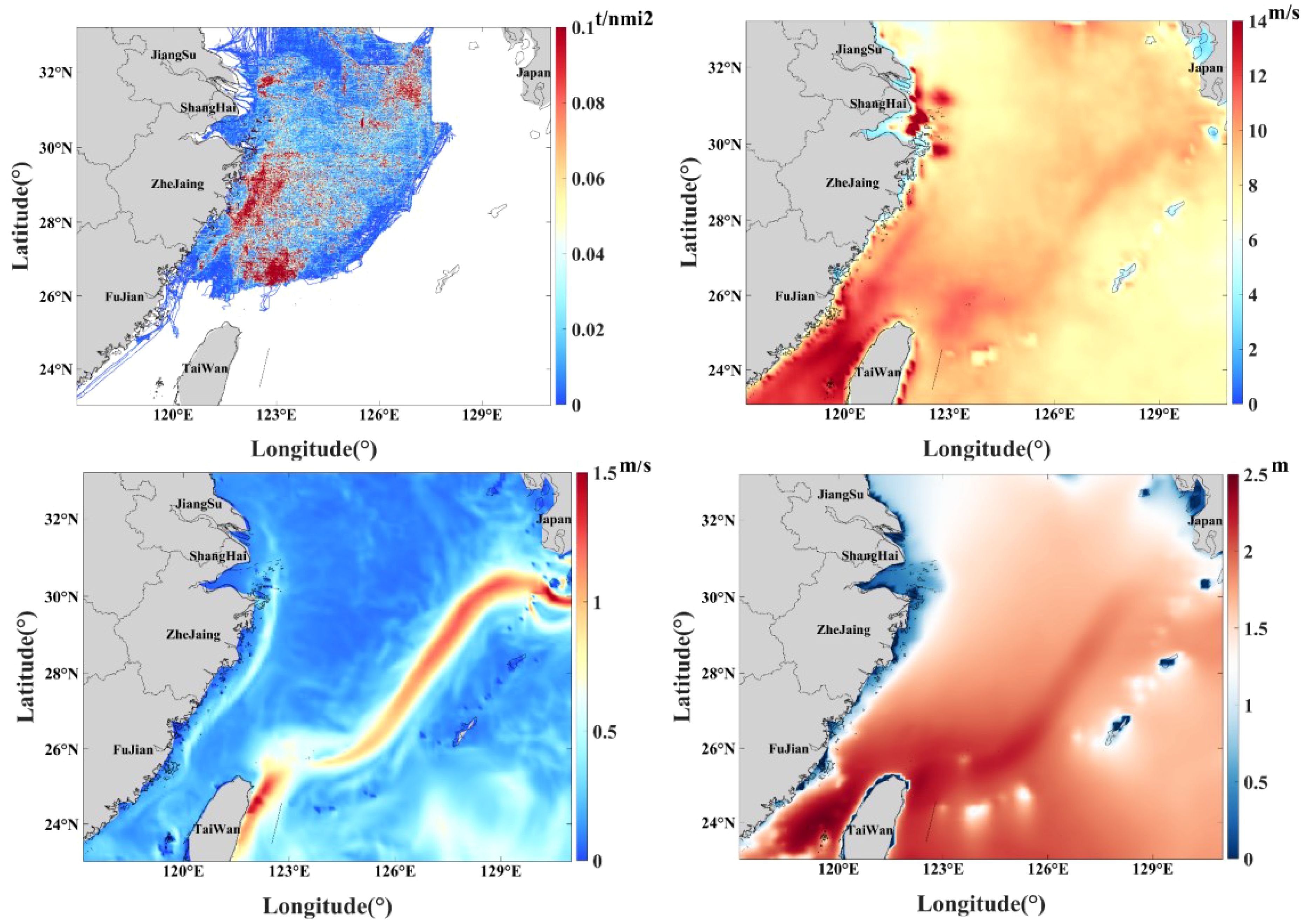
Figure 20 Schematic diagram of CO₂ emissions, wind velocity, flow velocity and wave height in January 2022.

Figure 21

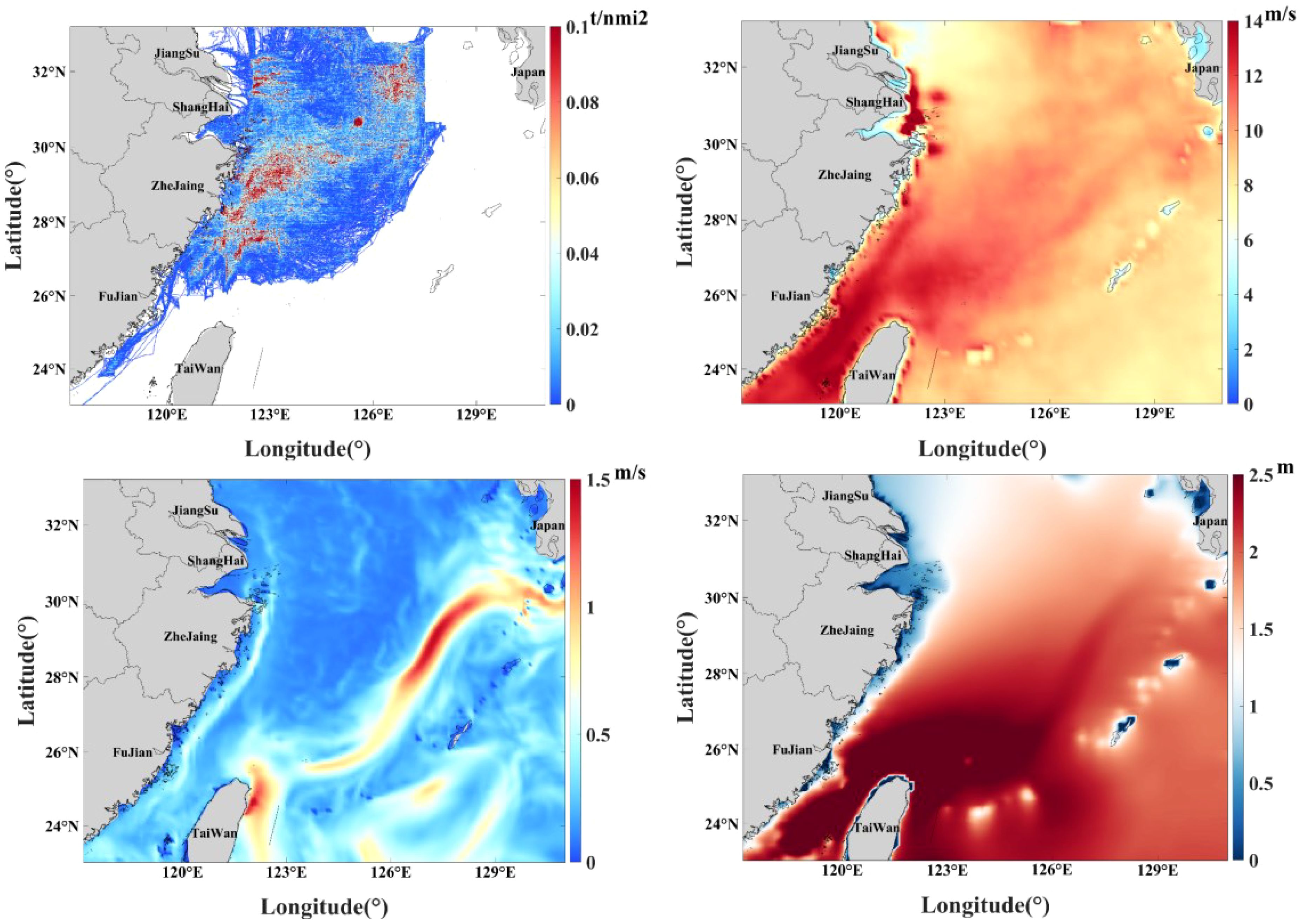
Figure 21 Schematic diagram of CO₂ emissions, wind velocity, flow velocity and wave height in February 2022.

Figure 22

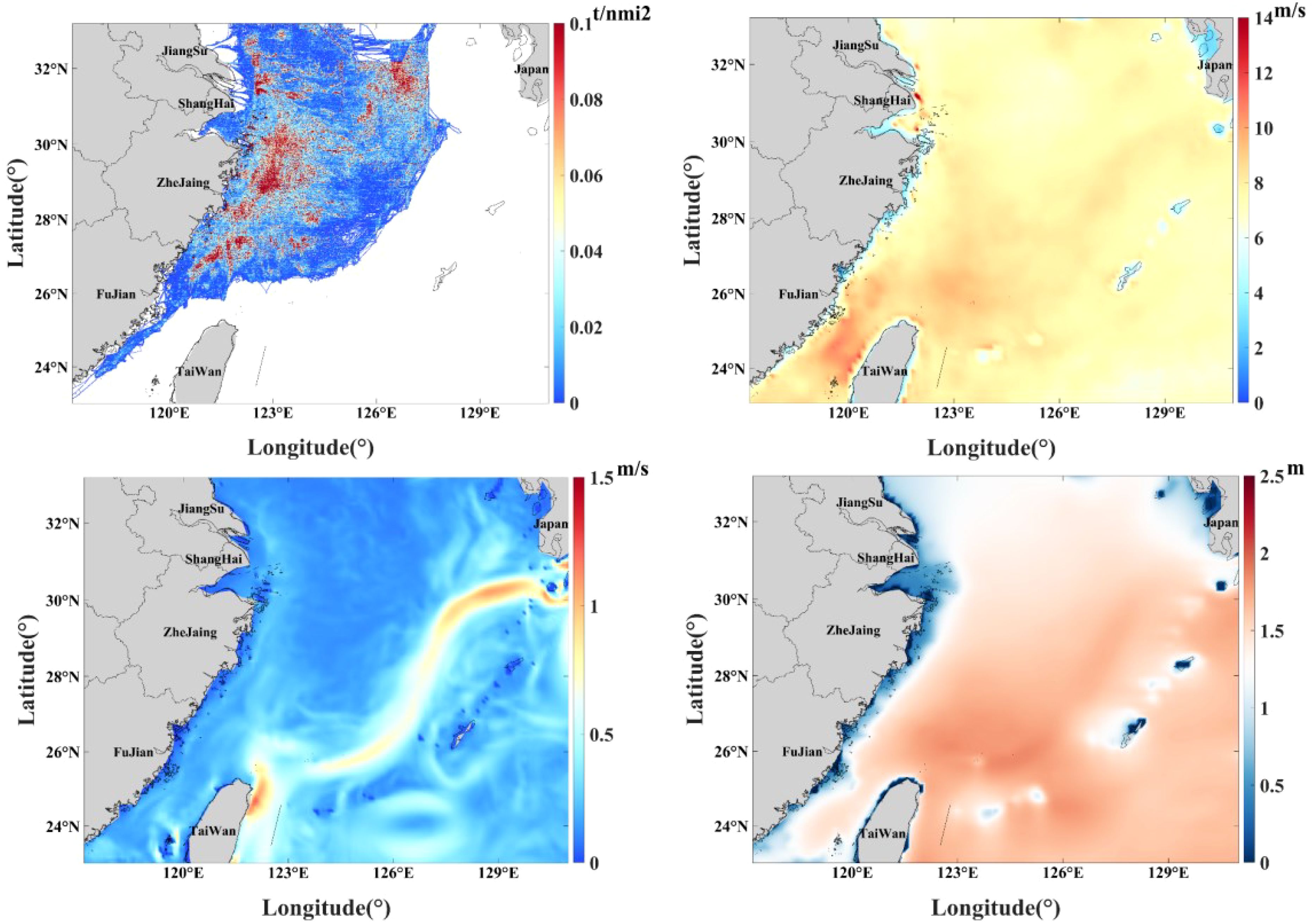
Figure 22 Schematic diagram of CO₂ emissions, wind velocity, flow velocity and wave height in March 2022.

Figure 23

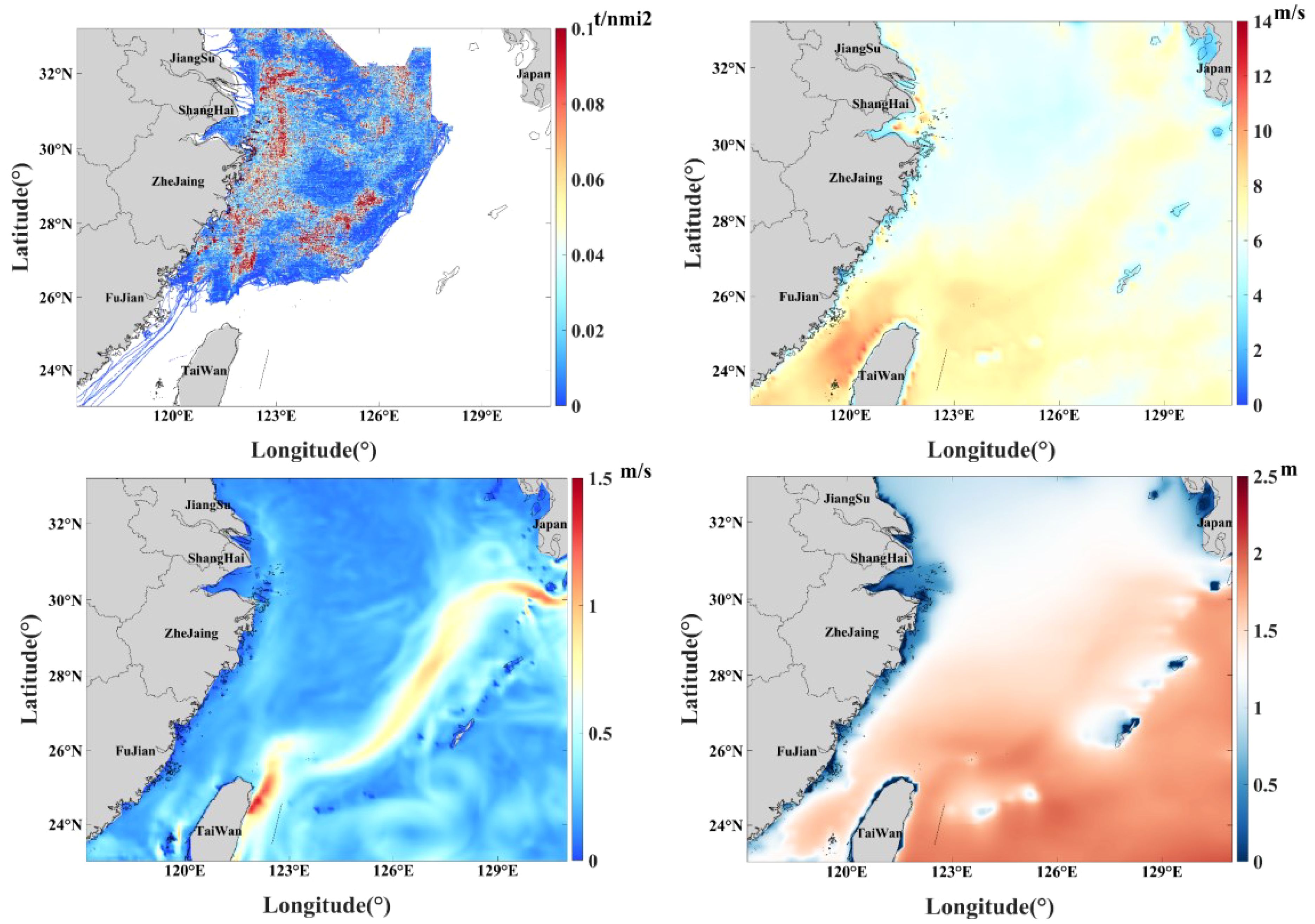
Figure 23 Schematic diagram of CO₂ emissions, wind velocity, flow velocity and wave height in April 2022.

6.4 Spatial distribution

6.4.1 Distribution of emissions at different distances from the coastline

Based on the different distances from the coastline, the East China Sea was divided into five sea areas, at 12 nautical miles, 36 nautical miles, 84 nautical miles, 180 nautical miles, and other sea areas from the coastline to the baselines outside the territorial sea. The specific distribution is shown in Figure 24. Emissions from fishing vessels in different sea areas at different distances from the coastline are shown in Table 7. Table 7 shows that most (over 80%) of the emissions from fishing vessels are in waters within 180 nautical miles from the coastline to the baseline of the territorial sea, and more than half (about 55%) of the emissions occur in waters within 84 nautical miles from the coastline to the baseline of the territorial sea. This indicates that most emissions from fishing vessels occur in waters close to the coastline.

Figure 24

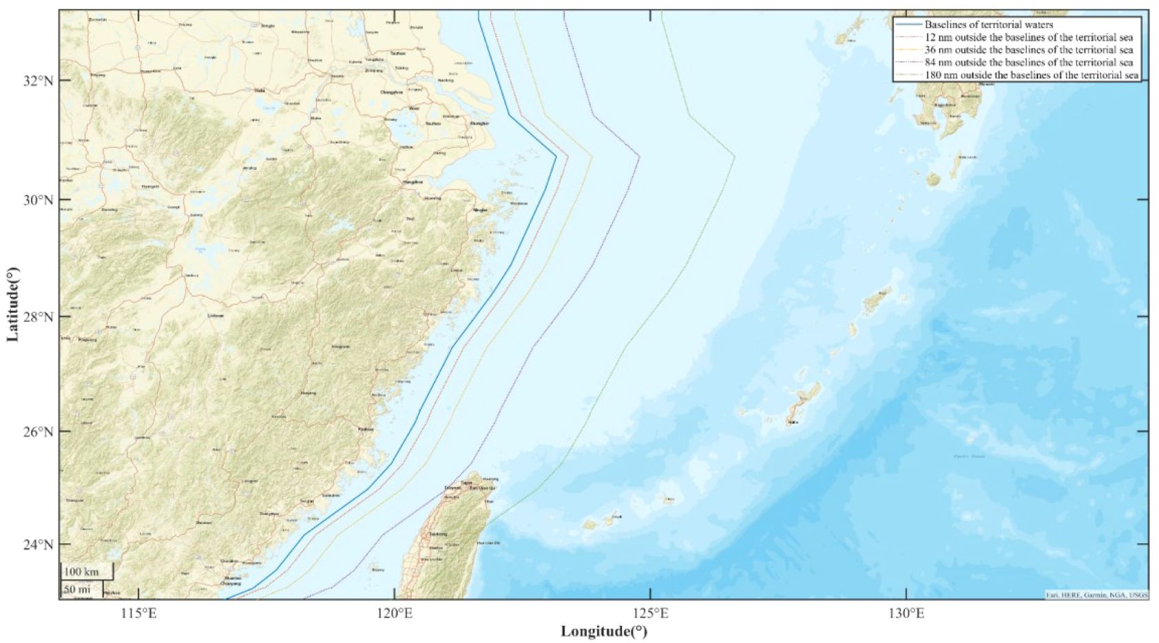
Figure 24 Sea areas at different distances from the coastline.

Table 7

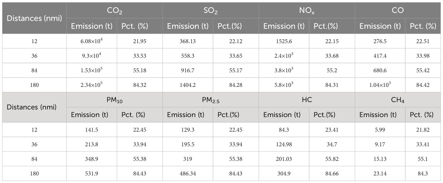
Table 7 Emissions in different distances from the baseline of the Chinese territorial sea.

6.4.2 Distribution of emissions from different fishing grounds

We counted the carbon emissions and emission intensity of 17 fishing grounds in the East China Sea. The details are shown in Table 8; Figure 25. Of these 17 fishing grounds, the largest emission from fishing vessels and the highest emission intensity is in the Yushan fishing ground, followed by the Zhoushan fishing ground, the Wentai fishing ground and the Yangtze River Estuary fishing ground. The three fishing grounds with the highest emissions and the highest emission intensity are all located in the coastal waters of Zhejiang. The emissions from fishing vessels in these three fishing grounds accounted for approximately 56% of the total emissions from fishing vessels in the East China Sea. The lowest emissions and emission intensity are in the Minnan fishing ground.

Table 8

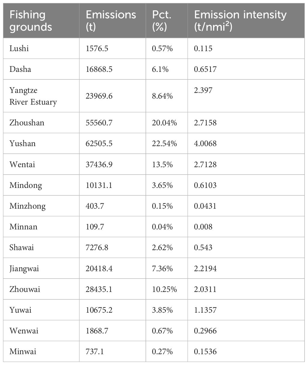
Table 8 CO₂ emissions, emission percentage and emission intensity from fishing vessels in different fishing grounds.

Figure 25

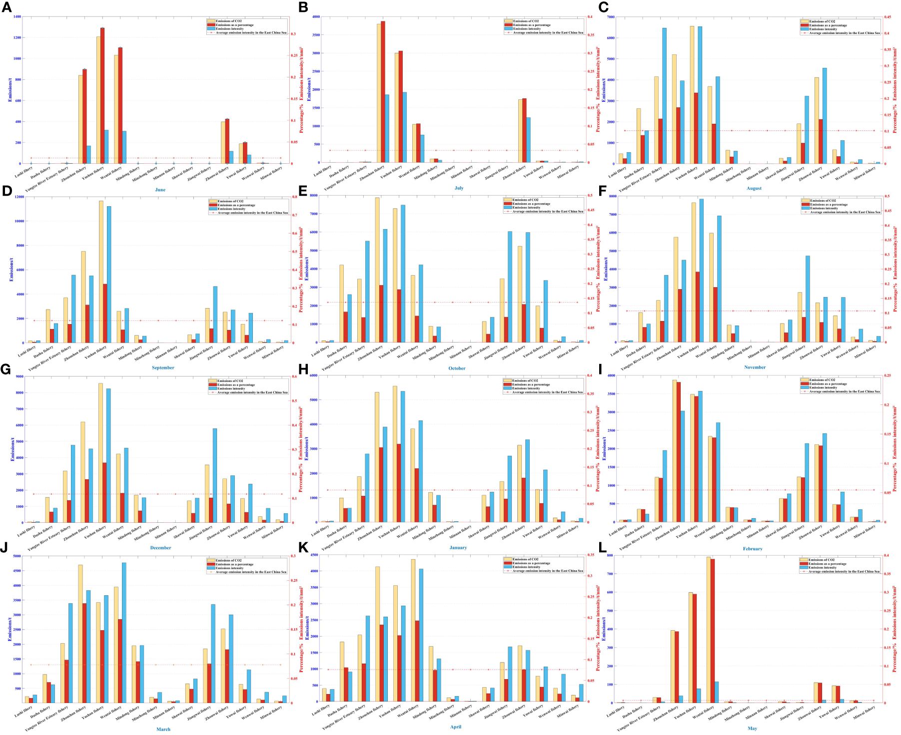
Figure 25 CO₂ emissions and emission intensity of fishing grounds by month. (A) in June 2021, (B) in July 2021, (C) in August 2021, (D) in September 2021, (E) in October 2021, (F) in November 2021, (G) in December 2021, (H) in January 2022, (I) in February 2022, (J) in March 2022, (K) in April 2022 and (L) in May 2022.

6.5 Distribution of emissions based on fishing hotspots

Pollutant emissions from fishing vessels vary with the load of the main engine (Fan et al., 2023), which is related to the speed of the vessel, according to Equation (3). Fishing vessel speed is positively correlated with vessel load and pollutant emissions. Sala et al. (2011) found that fishing vessels can save up to 15% of fuel by reducing their speed by half a knot. In fishing activities, there are three behavioral states: stationary anchoring, high-speed sailing and low-speed fishing. Emissions from fishing vessels are higher at high speeds and lower at low fishing speeds (Yan et al., 2022). Therefore, the total emission hotspot distribution cannot accurately indicate the fishing hotspot areas of fishing vessels. Thus, we used the simplest speed recognition method to distinguish the behavioral state of fishing vessels. The identification of fishing hotspot areas for fishing vessels is more accurately based on vessel emissions during low-speed fishing conditions. The speed identification method is a common traditional method to distinguish fishing vessel behavior based on their speed. This method is simple, effective and suitable for identifying fishing vessel behavior using big data (Yan et al., 2022). Considering the different types of fishing operations, we selected the four most common types of fishing vessels in the East China Sea: trawlers, driftnets, purse seines, and longliners. By analyzing the distribution of CO₂ emissions from these vessels during their fishing speed states (trawlers: 3≤v ≤ 5 (Liu et al., 2023b), i.e., the speed of the trawlers is greater than 3 knots but less than 5 knots, here “v” refers to the velocity of the fishing vessels; driftnets: 1≤v ≤ 3 (Sala et al., 2018), i.e., the speed of the driftnets is greater than 1 knots but less than 3 knots; purse-seines: 2≤v ≤ 4 (Hintzen et al., 2012), i.e., the speed of the purse-seines is greater than 2 knots but less than 4 knots; driftnets; longliners: 1≤v ≤ 3 (Campos et al., 2023), i.e., the speed of the longliners is greater than 1 knots but less than 3 knots), we examined the different fishing hotspots for these four types of vessels during the four seasons: spring (March-May), summer (June-August), autumn (September-November), and winter (December - February). We also analyzed the distribution of CO₂ emissions from fishing transport vessels.

The distribution of CO₂ emissions from different types of fishing vessels in the fishing state is shown in Figures 26–29. The figures show that the fishing area is the smallest in summer, due to the influence of the seasonal fishing moratorium system, and shrinks in other seasons over time, with the gradual depletion of fishery resources. The distribution of CO₂ emissions from the fishing transportation vessels, in each season, is shown in Figure 30. The figure shows that the distribution of emissions from catch-and-carry vessels changes with the change in fishery resources. According to the emission distribution of fishing transportation vessels, it is evident that Zhejiang Province is the main consumption point of fishery resources in the East China Sea, followed by Jiangsu Province and Fujian Province.

Figure 26

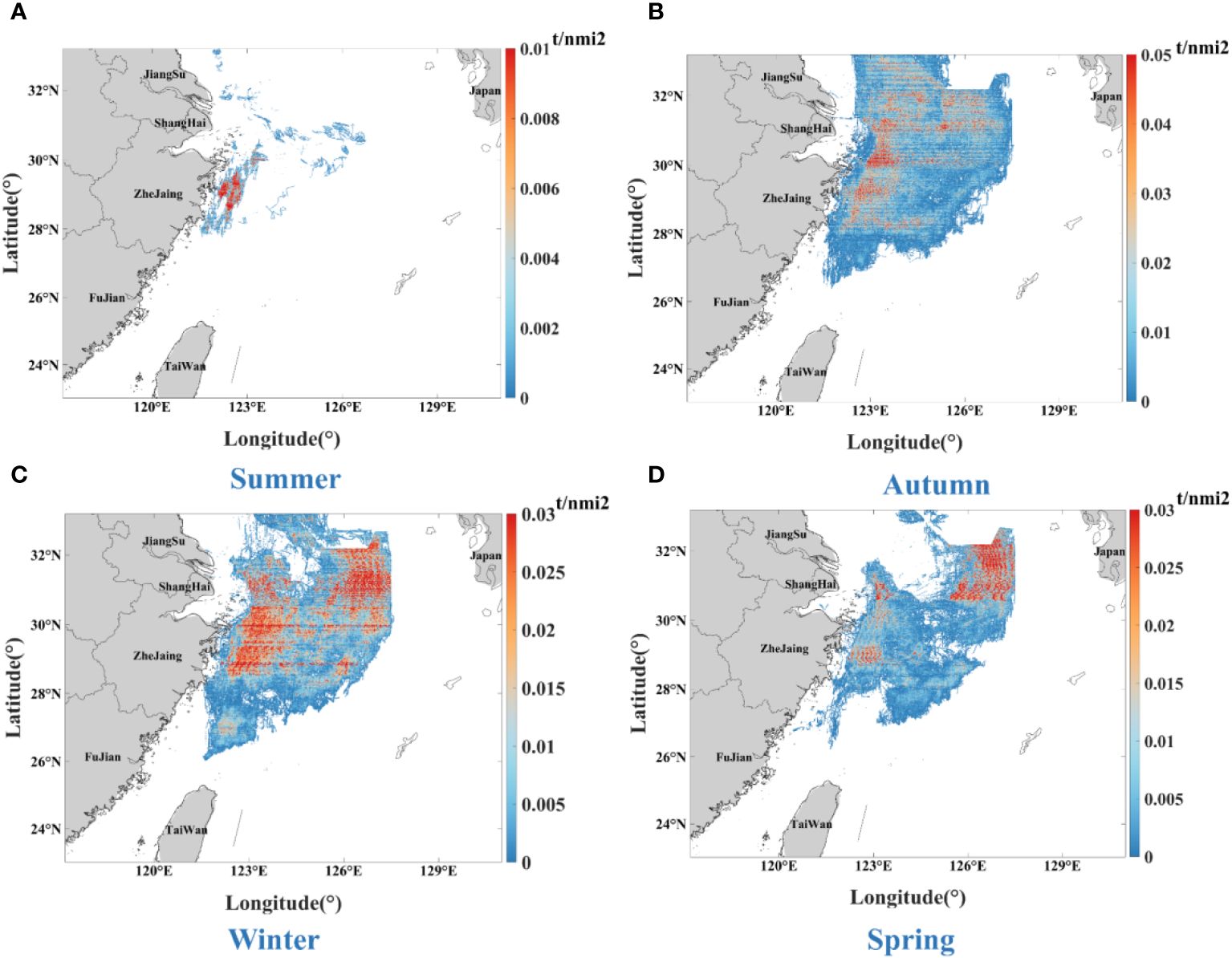
Figure 26 Hot spot areas for trawler vessels by season. (A) in Summer, (B) in Autumn, (C) in Winter and (D) in Spring.

Figure 27

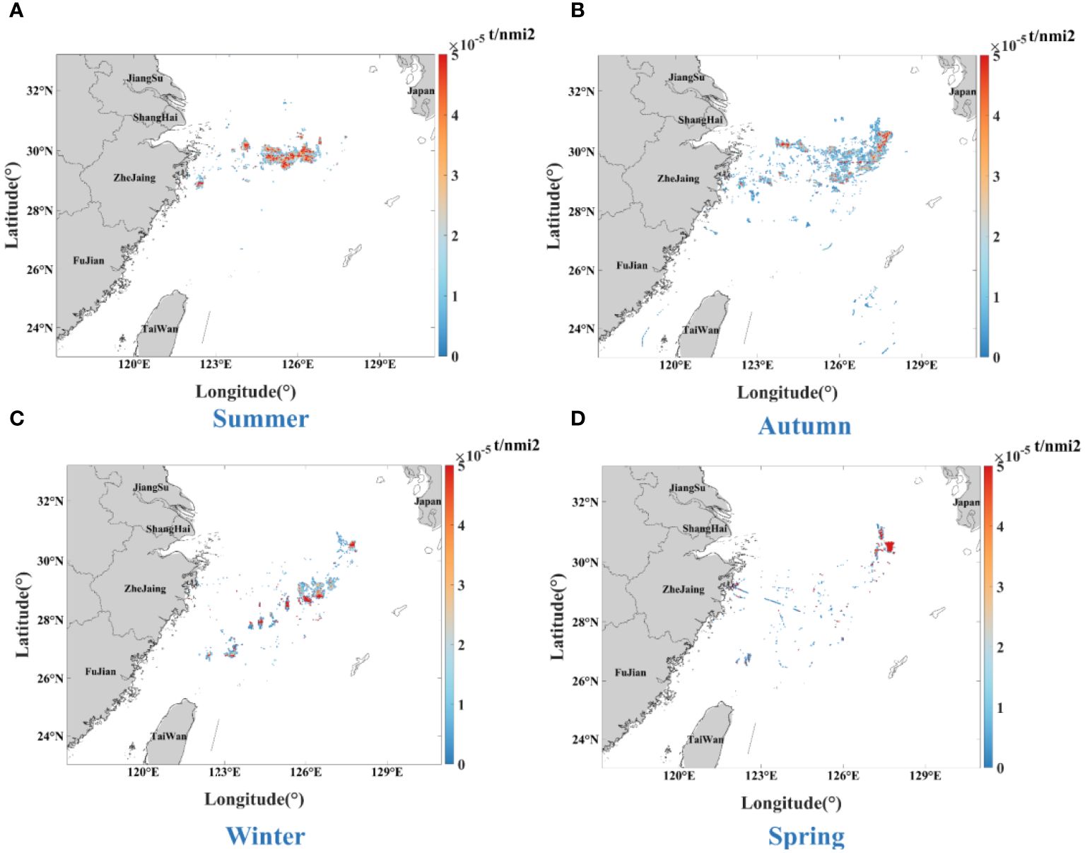
Figure 27 Hot spot areas for longliners vessels by season. (A) in Summer, (B) in Autumn, (C) in Winter and (D) in Spring.

Figure 28

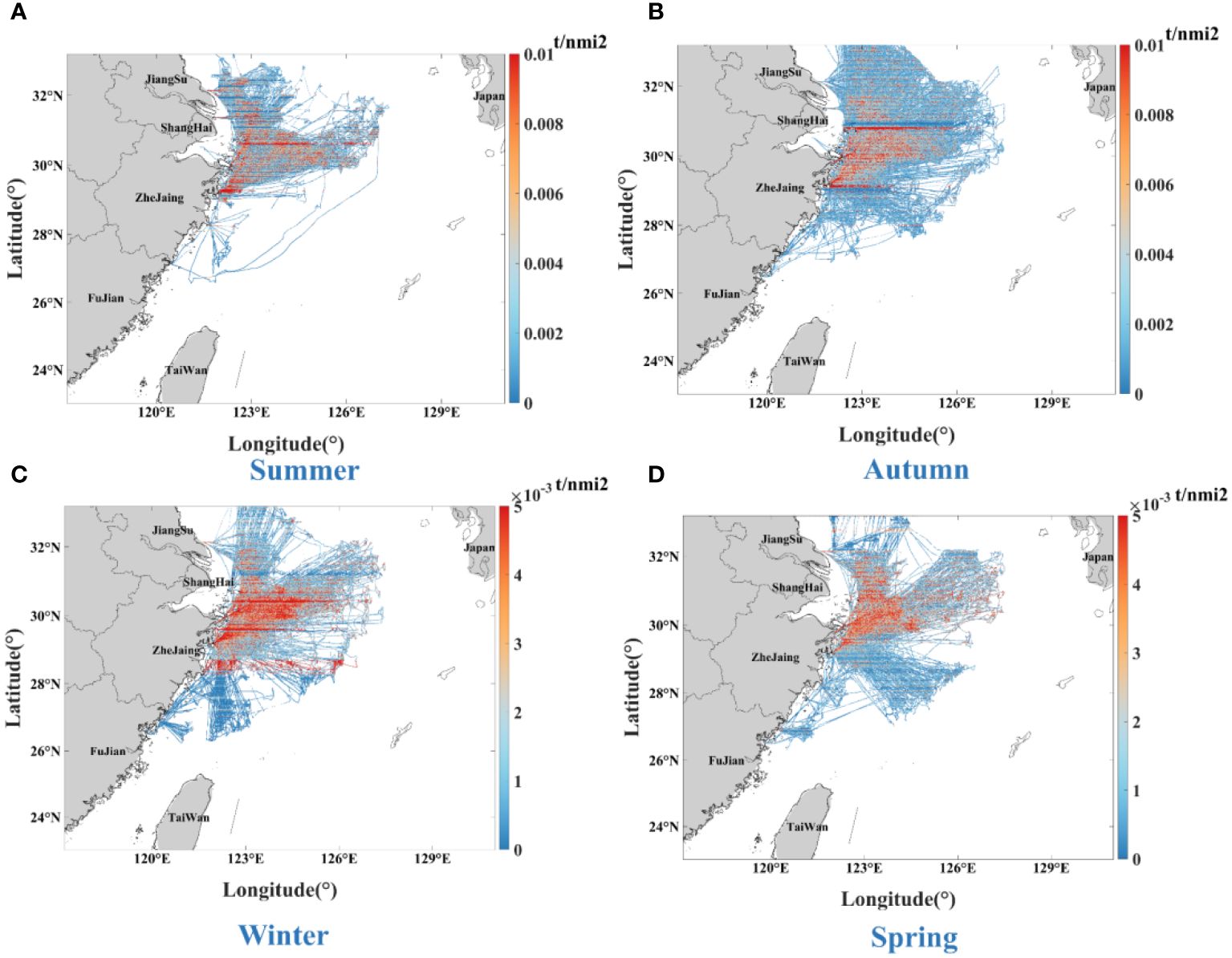
Figure 28 Hot spot areas for transportation vessels by season. (A) in Summer, (B) in Autumn, (C) in Winter and (D) in Spring.

Figure 29

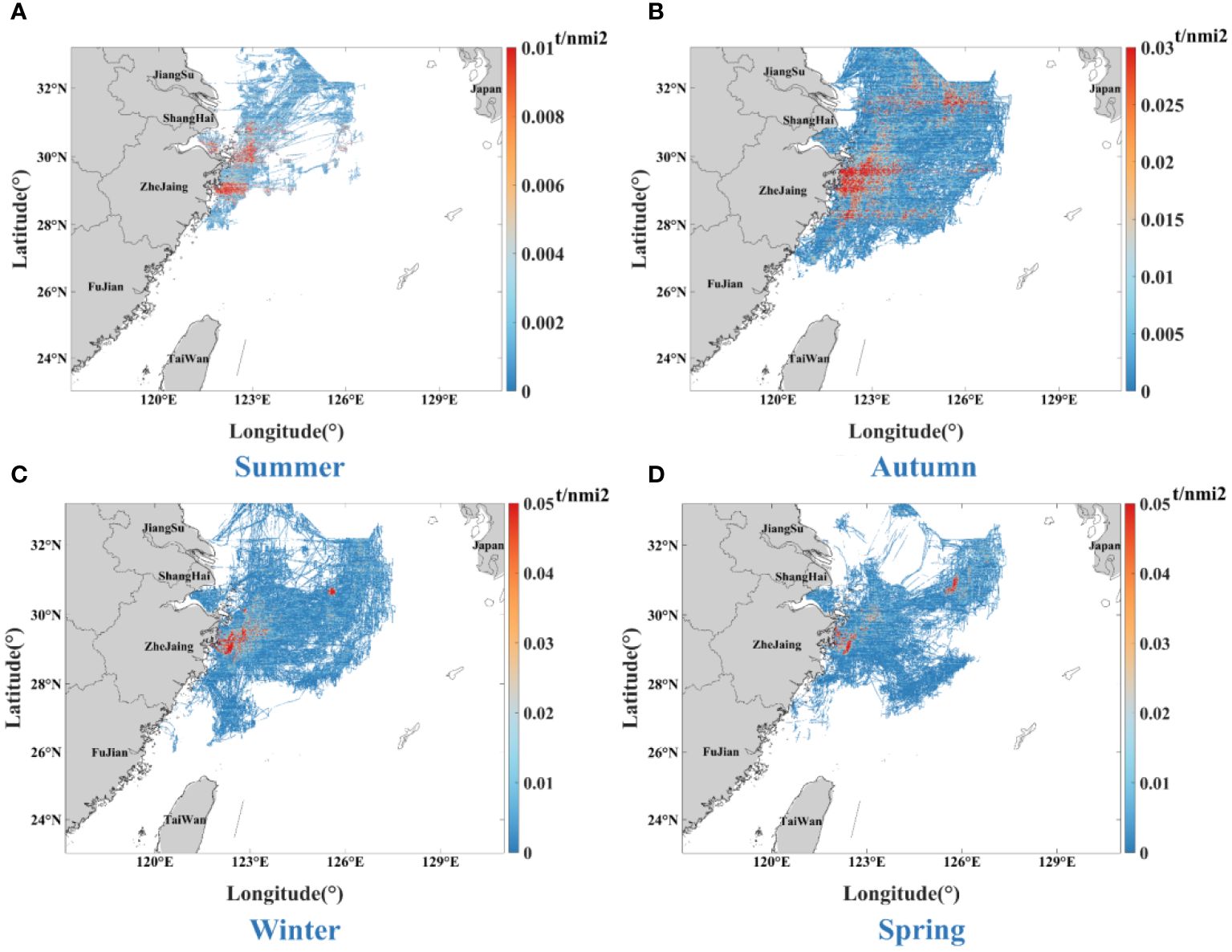
Figure 29 Hot spot areas for drift-net vessels by season. (A) in Summer, (B) in Autumn, (C) in Winter and (D) in Spring.

Figure 30

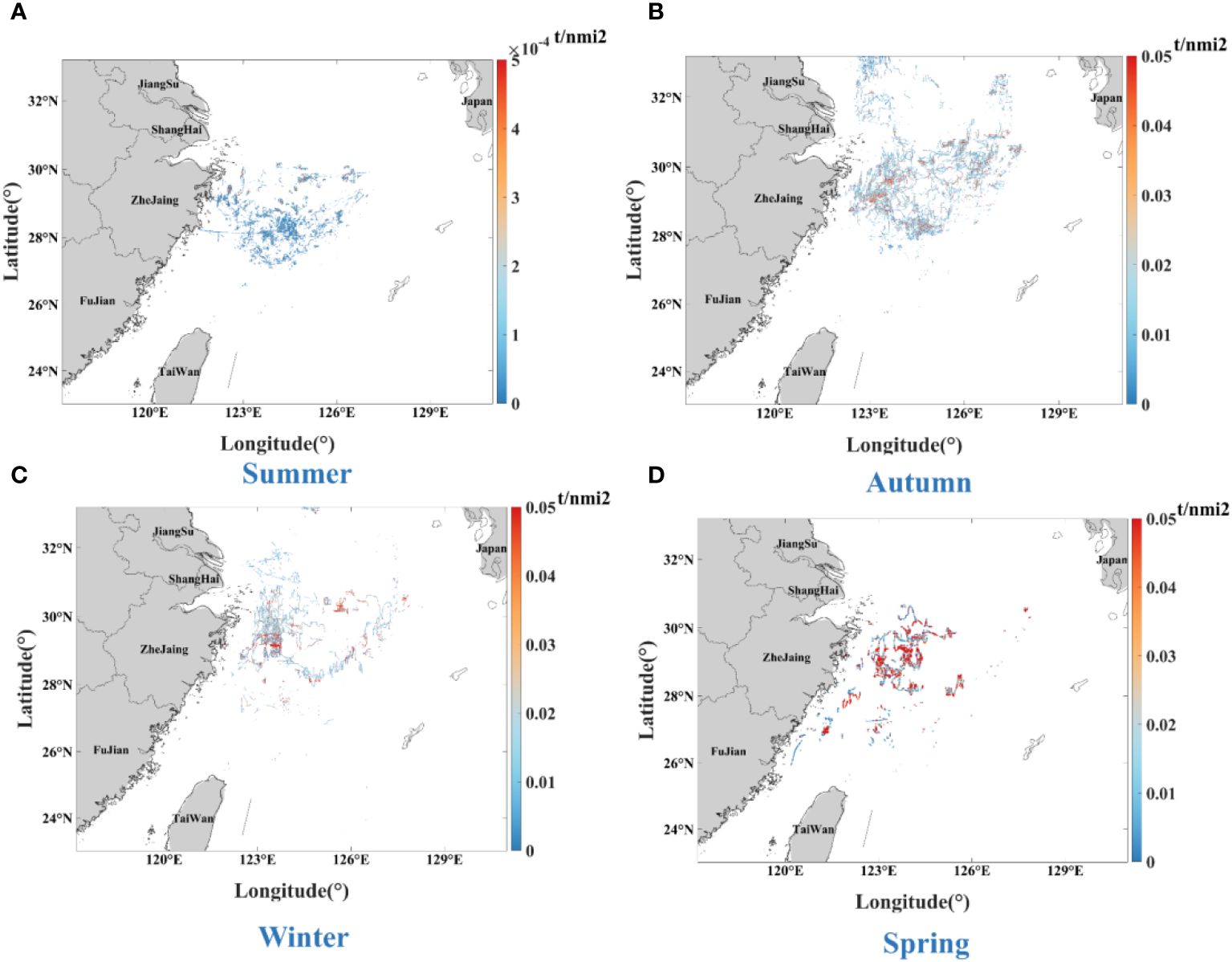
Figure 30 Hot spot areas for seine vessels by season. (A) in Summer, (B) in Autumn, (C) in Winter and (D) in Spring.

7 Conclusions

In this study, a fishing vessel emission estimation framework was established based on Beidou VMS big data using the bottom-up dynamic method. The framework was applied to Zhejiang fishing vessels in the fishing grounds of the East China Sea and established an emission inventory and the spatial-temporal distribution from 1st June 2021 to 31st May 2022.

The findings indicate that the large quantity of fishing vessels and high main engine power in Zhejiang Province leads to relatively high emissions from fishing vessels. In conclusion, this study demonstrates that using activity-based bottom-up methods and VMS data is an effective approach for investigating pollution emissions from fishing vessels in the East China Sea and is applicable in areas where small-scale fishing boats are prevalent. By addressing this issue, we can strive towards creating a more sustainable future for our oceans and marine ecosystems.

However, it is necessary to recognize the limitations of this study. First, the analysis only included Zhejiang Province fishing vessels in the East China Sea and may not be representative of all vessel types in China or other regions. Second, the accuracy of the emission factors used in this study may affect the estimation results. Finally, measures aimed at reducing pollution emissions from fishing vessels were not proposed, and further research and validation of these measures were not conducted.

Our future research will focus on the following areas: expanding the analysis to other regions and vessel types and improving the accuracy of the emission factors of fishing vessels by measuring them in the field with the help of experimental equipment. Next, we need to propose relevant emission reduction measures and verify their effectiveness. Finally, the diffusion of pollutant emissions from fishing vessels under different meteorological conditions in the East China Sea will be simulated by using meteorological simulation software or building meteorological models to assess their impacts on coastal air quality.

Data availability statement

The raw data supporting the conclusions of this article will be made available by the authors, without undue reservation.

Author contributions

KZ: Writing – original draft. QL: Writing – review & editing, Data curation, Formal analysis. FL: Writing – review & editing, Data curation, Investigation, Resources. HF: Writing – review & editing, Conceptualization, Funding acquisition, Methodology, Project administration, Supervision, Validation.

Funding

The author(s) declare financial support was received for the research, authorship, and/or publication of this article. This work was sponsored by the K. C. Wong Magna Fund at Ningbo University and the Natural Science Foundation of China (grant number 72271132) and 111 Project (grant number D21013).

Acknowledgments

The authors would like to thank the referees for their constructive comments on this paper. Their comments significantly increased the quality of this paper.

Conflict of interest

The authors declare that the research was conducted in the absence of any commercial or financial relationships that could be construed as a potential conflict of interest.

Publisher’s note

All claims expressed in this article are solely those of the authors and do not necessarily represent those of their affiliated organizations, or those of the publisher, the editors and the reviewers. Any product that may be evaluated in this article, or claim that may be made by its manufacturer, is not guaranteed or endorsed by the publisher.

References

Basurko O. C., Gabiña G., Lopez J., Granado I., Murua H., Fernandes J. A., et al. (2022). Fuel consumption of free-swimming school versus FAD strategies in tropical tuna purse seine fishing. Fisheries Res. 245, 106139. doi: 10.1016/j.fishres.2021.106139

CrossRef Full Text | Google Scholar

Byrne C., Agnarsson S., Davidsdottir B. (2021). Fuel Intensity in Icelandic fisheries and opportunities to reduce emissions. Mar. Policy 127, 104448. doi: 10.1016/j.marpol.2021.104448

CrossRef Full Text | Google Scholar

Campos A., Leitão P., Sousa L., Gaspar P., Henriques V. (2023). Spatial patterns of fishing activity inside the Gorringe bank MPA based on VMS, AIS and e-logbooks data. Mar. Policy 147, 105356. doi: 10.1016/j.marpol.2022.105356

CrossRef Full Text | Google Scholar

Cavraro F., Monti M. A., Caccin A., Fiori F., Grati F., Russo E., et al. (2023). Is the Small-Scale Fishery more sustainable in terms of GHG emissions? A Case study Anal. Cent. Mediterr. Sea. Mar. Policy 148, 105474. doi: 10.1016/j.marpol.2023.105474

CrossRef Full Text | Google Scholar

Chang N.-N., Shiao J.-C., Gong G.-C. (2012). Diversity of demersal fish in the East China Sea: Implication of eutrophication and fishery. Continental Shelf Res. 47, 42–54. doi: 10.1016/j.csr.2012.06.011

CrossRef Full Text | Google Scholar

Chassot E., Antoine S., Guillotreau P., Lucas J., Assan C., Marguerite M., et al. (2021). Fuel consumption and air emissions in one of the world’s largest commercial fisheries. Environ. pollut. 273, 116454. doi: 10.1016/j.envpol.2021.116454

PubMed Abstract | CrossRef Full Text | Google Scholar

Chen D., Wang X., Li Y., Lang J., Zhou Y., Guo X., et al. (2017a). High-spatiotemporal-resolution ship emission inventory of China based on AIS data in 2014. Sci. Total Environ. 609, 776–787. doi: 10.1016/j.scitotenv.2017.07.051

PubMed Abstract | CrossRef Full Text | Google Scholar

Chen D., Wang X., Nelson P., Li Y., Zhao N., Zhao Y., et al. (2017b). Ship emission inventory and its impact on the PM 2.5 air pollution in Qingdao Port, North China. Atmospheric Environ. 166, 351–361. doi: 10.1016/j.atmosenv.2017.07.021

CrossRef Full Text | Google Scholar

Chen S., Meng Q., Jia P., Kuang H. (2021). An operational-mode-based method for estimating ship emissions in port waters. Transportation Res. Part D: Transport Environ. 101, 103080. doi: 10.1016/j.trd.2021.103080

CrossRef Full Text | Google Scholar

Chen X., Yang J. (2024). Analysis of the uncertainty of the AIS-based bottom-up approach for estimating ship emissions. Mar. pollut. Bull. 199, 115968. doi: 10.1016/j.marpolbul.2023.115968

PubMed Abstract | CrossRef Full Text | Google Scholar

Chen X., Di Q., Hou Z., Yu Z. (2022). Measurement of carbon emissions from marine fisheries and system dynamics simulation analysis: China’s northern marine economic zone case. Mar. Policy 145, 105279. doi: 10.1016/j.marpol.2022.105279

CrossRef Full Text | Google Scholar

Coello J., Williams I., Hudson D. A., Kemp S. (2015). An AIS-based approach to calculate atmospheric emissions from the UK fishing fleet. Atmospheric Environ. 114, 1–7. doi: 10.1016/j.atmosenv.2015.05.011

CrossRef Full Text | Google Scholar

Driscoll J., Tyedmers P. (2010). Fuel use and greenhouse gas emission implications of fisheries management: the case of the new england atlantic herring fishery. Mar. Policy 34, 353–359. doi: 10.1016/j.marpol.2009.08.005

CrossRef Full Text | Google Scholar

Eyring V., Isaksen I. S. A., Berntsen T., Collins W. J., Corbett J. J., Endresen O., et al. (2010). Transport impacts on atmosphere and climate: Shipping. Atmospheric Environ. 44, 4735–4771. doi: 10.1016/j.atmosenv.2009.04.059

CrossRef Full Text | Google Scholar

Fan A., Yan J., Xiong Y., Shu Y., Fan X., Wang Y., et al. (2023). Characteristics of real-world ship energy consumption and emissions based on onboard testing. Mar. pollut. Bull. 194, 115411. doi: 10.1016/j.marpolbul.2023.115411

PubMed Abstract | CrossRef Full Text | Google Scholar

Fan Q., Zhang Y., Ma W., Ma H., Feng J., Yu Q., et al. (2016). Spatial and seasonal dynamics of ship emissions over the Yangtze River delta and East China Sea and their potential environmental influence. Environ. Sci. Technol. 50, 1322–1329. doi: 10.1021/acs.est.5b03965

PubMed Abstract | CrossRef Full Text | Google Scholar

Feng H., Grifoll M., Yang Z., Zheng P. (2022). Collision risk assessment for ships’ routeing waters: An information entropy approach with Automatic Identification System (AIS) data. Ocean Coast. Manage. 224, 106184. doi: 10.1016/j.ocecoaman.2022.106184

CrossRef Full Text | Google Scholar

Fuentes G., Adland R. (2023). Greenhouse gas mitigation at maritime chokepoints: The case of the Panama Canal. Transportation Res. Part D: Transport Environ. 118, 103694. doi: 10.1016/j.trd.2023.103694

CrossRef Full Text | Google Scholar

Gan L., Che W., Zhou M., Zhou C., Zheng Y., Zhang L., et al. (2022). Ship exhaust emission estimation and analysis using Automatic Identification System data: The west area of Shenzhen port, China, as a case study. Ocean Coast. Manage. 226, 106245. doi: 10.1016/j.ocecoaman.2022.106245

CrossRef Full Text | Google Scholar

Garnett T. (2011). Where are the best opportunities for reducing greenhouse gas emissions in the food system (including the food chain)? Food Policy 36, S23–S32. doi: 10.1016/j.foodpol.2010.10.010

CrossRef Full Text | Google Scholar

Greer K., Zeller D., Woroniak J., Coulter A., Winchester M., Palomares M. L. D., et al. (2019). Global trends in carbon dioxide (CO2) emissions from fuel combustion in marine fisheries from 1950 to 2016. Mar. Policy 107, 103382. doi: 10.1016/j.marpol.2018.12.001

CrossRef Full Text | Google Scholar

Grigoriadis A., Mamarikas S., Ioannidis I., Majamäki E., Jalkanen J.-P., Ntziachristos L. (2021). Development of exhaust emission factors for vessels: A review and meta-analysis of available data. Atmospheric Environment: X 12, 100142. doi: 10.1016/j.aeaoa.2021.100142

CrossRef Full Text | Google Scholar

Hintzen N. T., Bastardie F., Beare D., Piet G. J., Ulrich C., Deporte N., et al. (2012). VMStools: Open-source software for the processing, analysis and visualisation of fisheries logbook and VMS data. Fisheries Res. 115-116, 31–43. doi: 10.1016/j.fishres.2011.11.007

CrossRef Full Text | Google Scholar

Hintzen N. T., Piet G. J., Brunel T. (2010). Improved estimation of trawling tracks using cubic Hermite spline interpolation of position registration data. Fisheries Res. 101, 108–115. doi: 10.1016/j.fishres.2009.09.014

CrossRef Full Text | Google Scholar

Huang H., Zhou C., Huang L., Xiao C., Wen Y., Li J., et al. (2022). Inland ship emission inventory and its impact on air quality over the middle Yangtze River, China. Sci. Total Environ. 843, 156770. doi: 10.1016/j.scitotenv.2022.156770

PubMed Abstract | CrossRef Full Text | Google Scholar

Huang L., Wen Y., Geng X., Zhou C., Xiao C., Zhang F. (2017). Estimation and spatio-temporal analysis of ship exhaust emission in a port area. Ocean Eng. 140, 401–411. doi: 10.1016/j.oceaneng.2017.06.015

CrossRef Full Text | Google Scholar

Huang L., Wen Y., Zhang Y., Zhou C., Zhang F., Yang T. (2020). Dynamic calculation of ship exhaust emissions based on real-time AIS data. Transportation Res. Part D: Transport Environ. 80, 102277. doi: 10.1016/j.trd.2020.102277

CrossRef Full Text | Google Scholar

Issifu I., Alava J. J., Lam V. W. Y., Sumaila U. R. (2022). Impact of ocean warming, overfishing and mercury on European fisheries: A risk assessment and policy solution framework. Front. Mar. Sci. 8, 770805. doi: 10.3389/fmars.2021.770805

CrossRef Full Text | Google Scholar

Jalkanen J. P., Brink A., Kalli J., Pettersson H., Kukkonen J., Stipa T. (2009). A modelling system for the exhaust emissions of marine traffic and its application in the Baltic Sea area. Atmos. Chem. Phys. 9, 9209–9223. doi: 10.5194/acp-9-9209-2009

CrossRef Full Text | Google Scholar

Jalkanen J. P., Johansson L., Kukkonen J., Brink A., Kalli J., Stipa T. (2012). Extension of an assessment model of ship traffic exhaust emissions for particulate matter and carbon monoxide. Atmos. Chem. Phys. 12, 2641–2659. doi: 10.5194/acp-12-2641-2012

CrossRef Full Text | Google Scholar

Joo R., Salcedo O., Gutierrez M., Fablet R., Bertrand S. (2015). Defining fishing spatial strategies from VMS data: Insights from the world's largest monospecific fishery. Fisheries Res. 164, 223–230. doi: 10.1016/j.fishres.2014.12.004

CrossRef Full Text | Google Scholar

Lee S., Park Y. K., Park H. (2017). The complex legal status of the Current Fishing Pattern Zone in the East China Sea. Mar. Policy 81, 219–228. doi: 10.1016/j.marpol.2017.03.021

CrossRef Full Text | Google Scholar

Li G., Li D., Xiong Y., Zhong X., Shi J., Zhang H., et al. (2023a). Dynamic valuation of the provisioning services of marine fisheries ecosystem based on BeiDou VMS data: A case study of TACs project for Acetes chinensis in the Yellow Sea. Ocean Coast. Manage. 243, 106773. doi: 10.1016/j.ocecoaman.2023.106773

CrossRef Full Text | Google Scholar

Li H., Jia P., Wang X., Yang Z., Wang J., Kuang H. (2023b). Ship carbon dioxide emission estimation in coastal domestic emission control areas using high spatial-temporal resolution data: A China case. Ocean Coast. Manage. 232, 106419. doi: 10.1016/j.ocecoaman.2022.106419

CrossRef Full Text | Google Scholar

Lin Q., Yin B., Zhang X., Grifoll M., Feng H. (2023). Evaluation of ship collision risk in ships’ routeing waters: A Gini coefficient approach using AIS data. Physica A: Stat. Mechanics its Appl. 624, 128936. doi: 10.1016/j.physa.2023.128936

CrossRef Full Text | Google Scholar

Liu G., Xu Y., Ge W., Yang X., Su X., Shen B., et al. (2023a). How can marine fishery enable low carbon development in China? Based on system dynamics simulation analysis. Ocean Coast. Manage. 231, 106382. doi: 10.1016/j.ocecoaman.2022.106382

CrossRef Full Text | Google Scholar

Liu H., Fu M., Jin X., Shang Y., Shindell D., Faluvegi G., et al. (2016). Health and climate impacts of ocean-going vessels in East Asia. Nat. Climate Change 6, 1037–1041. doi: 10.1038/nclimate3083

CrossRef Full Text | Google Scholar

Liu H., Jin X., Wu L., Wang X., Fu M., Lv Z., et al. (2018). The impact of marine shipping and its DECA control on air quality in the Pearl River Delta, China. Sci. Total Environ. 625, 1476–1485. doi: 10.1016/j.scitotenv.2018.01.033

PubMed Abstract | CrossRef Full Text | Google Scholar

Liu Q., Chen Y., Wang J., Miao H., Wang Y. (2023b). An example of fishery yield predictions from VMS-based navigational characteristics applied to double trawlers in China. Fisheries Res. 261, 106614. doi: 10.1016/j.fishres.2023.106614

CrossRef Full Text | Google Scholar

Longépé N., Hajduch G., Ardianto R., Nhunfat B., Marzuki M. I., Fablet R., et al. (2018). Completing fishing monitoring with spaceborne Vessel Detection System (VDS) and Automatic Identification System (AIS) to assess illegal fishing in Indonesia. Mar. pollut. Bull. 131, 33–39. doi: 10.1016/j.marpolbul.2017.10.016

PubMed Abstract | CrossRef Full Text | Google Scholar

Nishi R., Watanabe T. (2022). System-size dependence of a jam-absorption driving strategy to remove traffic jam caused by a sag under the presence of traffic instability. Physica A: Stat. Mechanics its Appl. 600, 127512. doi: 10.1016/j.physa.2022.127512

CrossRef Full Text | Google Scholar

Parker R. W. R., Blanchard J. L., Gardner C., Green B. S., Hartmann K., Tyedmers P. H., et al. (2018). Fuel use and greenhouse gas emissions of world fisheries. Nat. Climate Change 8, 333–337. doi: 10.1038/s41558-018-0117-x

CrossRef Full Text | Google Scholar

Peng X., Wen Y., Wu L., Xiao C., Zhou C., Han D. (2020). A sampling method for calculating regional ship emission inventories. Transportation Res. Part D: Transport Environ. 89, 102617. doi: 10.1016/j.trd.2020.102617

CrossRef Full Text | Google Scholar

Qian J., Li J., Zhang K., Qiu Y., Cai Y., Wu Q., et al. (2022). Spatial–temporal distribution of large-size light falling-net fisheries in the South China Sea. Front. Mar. Sci. 9, 1075855. doi: 10.3389/fmars.2022.1075855

CrossRef Full Text | Google Scholar

Sala A., Damalas D., Labanchi L., Martinsohn J., Moro F., Sabatella R., et al. (2022). Energy audit and carbon footprint in trawl fisheries. Sci. Data 9, 428. doi: 10.1038/s41597-022-01478-0

PubMed Abstract | CrossRef Full Text | Google Scholar

Sala A., De Carlo F., Buglioni G., Lucchetti A. (2011). Energy performance evaluation of fishing vessels by fuel mass flow measuring system. Ocean Eng. 38, 804–809. doi: 10.1016/j.oceaneng.2011.02.004

CrossRef Full Text | Google Scholar

Sala A., Lucchetti A., Sartor P. (2018). Technical solutions for European small-scale driftnets. Mar. Policy 94, 247–255. doi: 10.1016/j.marpol.2018.05.019

CrossRef Full Text | Google Scholar

Samy-Kamal M., Forcada A., Lizaso J. L. S. (2015). Effects of seasonal closures in a multi-specific fishery. Fisheries Res. 172, 303–317. doi: 10.1016/j.fishres.2015.07.027

CrossRef Full Text | Google Scholar

Shanthi T. S., Dheepanbalaji L., Priya R., Ambeth Kumar V. D., Kumar A., Sindhu P., et al. (2022). Illegal fishing, anomalous vessel behavior detection through automatic identification system. Materials Today: Proc. 62, 4685–4690. doi: 10.1016/j.matpr.2022.03.127

CrossRef Full Text | Google Scholar

Topic T., Murphy A. J., Pazouki K., Norman R. (2021). Assessment of ship emissions in coastal waters using spatial projections of ship tracks, ship voyage and engine specification data. Cleaner Eng. Technol. 2, 100089. doi: 10.1016/j.clet.2021.100089

CrossRef Full Text | Google Scholar

Tyedmers P. H., Watson R., Pauly D. (2005). Fueling global fishing fleets. Ambio 34, 635–638. doi: 10.1579/0044-7447-34.8.635

PubMed Abstract | CrossRef Full Text | Google Scholar

Tzannatos E. (2010). Ship emissions and their externalities for Greece. Atmospheric Environ. 44, 2194–2202. doi: 10.1016/j.atmosenv.2010.03.018

CrossRef Full Text | Google Scholar

Walker E., Bez N. (2010). A pioneer validation of a state-space model of vessel trajectories (VMS) with observers’ data. Ecol. Model. 221, 2008–2017. doi: 10.1016/j.ecolmodel.2010.05.007

CrossRef Full Text | Google Scholar

Wan Z., Ji S., Liu Y., Zhang Q., Chen J., Wang Q. (2020). Shipping emission inventories in China's Bohai Bay, Yangtze River Delta, and Pearl River Delta in 2018. Mar. pollut. Bull. 151, 110882. doi: 10.1016/j.marpolbul.2019.110882

PubMed Abstract | CrossRef Full Text | Google Scholar

Wang L., Du W., Shen H., Chen Y., Zhu X., Yun X., et al. (2022). Unexpected methane emissions from old small fishing vessels in China. Front. Mar. Sci. 10, 907868. doi: 10.3389/fenvs.2022.907868

CrossRef Full Text | Google Scholar

Wang L., Li Y. (2023). Estimation methods and reduction strategies of port carbon emissions - what literatures say? Mar. pollut. Bull. 195, 115451. doi: 10.1016/j.marpolbul.2023.115451

PubMed Abstract | CrossRef Full Text | Google Scholar

Wang Q., Wang S. (2022). Carbon emission and economic output of China’s marine fishery – A decoupling efforts analysis. Mar. Policy 135, 104831. doi: 10.1016/j.marpol.2021.104831

CrossRef Full Text | Google Scholar

Winther M., Christensen J. H., Plejdrup M. S., Ravn E. S., Eriksson Ó. F., Kristensen H. O. (2014). Emission inventories for ships in the arctic based on satellite sampled AIS data. Atmospheric Environ. 91, 1–14. doi: 10.1016/j.atmosenv.2014.03.006

CrossRef Full Text | Google Scholar

Wu Y., Liu D., Wang X., Li S., Zhang J., Qiu H., et al. (2021). Ambient marine shipping emissions determined by vessel operation mode along the East China Sea. Sci. Total Environ. 769, 144713. doi: 10.1016/j.scitotenv.2020.144713

PubMed Abstract | CrossRef Full Text | Google Scholar

Yan Z., He R., Ruan X., Yang H. (2022). Footprints of fishing vessels in Chinese waters based on automatic identification system data. J. Sea Res. 187, 102255. doi: 10.1016/j.seares.2022.102255

CrossRef Full Text | Google Scholar

Yang L., Zhang Q., Zhang Y., Lv Z., Wang Y., Wu L., et al. (2021). An AIS-based emission inventory and the impact on air quality in Tianjin port based on localized emission factors. Sci. Total Environ. 783, 146869. doi: 10.1016/j.scitotenv.2021.146869

PubMed Abstract | CrossRef Full Text | Google Scholar

Ye J., Chen J., Wen H., Wan Z., Tang T. (2022). Emissions assessment of bulk carriers in China's east Coast-Yangtze River maritime network based on different shipping modes. Ocean Eng. 249, 110903. doi: 10.1016/j.oceaneng.2022.110903

CrossRef Full Text | Google Scholar

Yoo S.-L. (2019). Network analysis by fishing type for fishing vessel rescue. Physica A: Stat. Mechanics its Appl. 514, 892–901. doi: 10.1016/j.physa.2018.09.139

CrossRef Full Text | Google Scholar

Zhang F., Chen Y., Chen Q., Feng Y., Shang Y., Yang X., et al. (2018). Real-world emission factors of gaseous and particulate pollutants from marine fishing boats and their total emissions in China. Environ. Sci. Technol. 52, 4910–4919. doi: 10.1021/acs.est.7b04002

PubMed Abstract | CrossRef Full Text | Google Scholar

Zhang F., Chen Y., Tian C., Wang X., Huang G., Fang Y., et al. (2014). Identification and quantification of shipping emissions in Bohai Rim, China. Sci. Total Environ. 497-498, 570–577. doi: 10.1016/j.scitotenv.2014.08.016

PubMed Abstract | CrossRef Full Text | Google Scholar

Zhang X., Wang C., Jiang L., An L., Yang R. (2021). Collision-avoidance navigation systems for Maritime Autonomous Surface Ships: A state of the art survey. Ocean Eng. 235, 109380. doi: 10.1016/j.oceaneng.2021.109380

CrossRef Full Text | Google Scholar

Zhang Y., Yang X., Brown R., Yang L., Morawska L., Ristovski Z., et al. (2017). Shipping emissions and their impacts on air quality in China. Sci. Total Environ. 581-582, 186–198. doi: 10.1016/j.scitotenv.2016.12.098

PubMed Abstract | CrossRef Full Text | Google Scholar

Zhao Z., Hong F., Huang H., Liu C., Feng Y., Guo Z. (2021). Short-term prediction of fishing effort distributions by discovering fishing chronology among trawlers based on VMS dataset. Expert Syst. Appl. 184, 115512. doi: 10.1016/j.eswa.2021.115512

CrossRef Full Text | Google Scholar

Zheng K., Zhang X., Wang C., Li Y., Cui J., Jiang L. (2024). Adaptive collision avoidance decisions in autonomous ship encounter scenarios through rule-guided vision supervised learning. Ocean Eng. 297, 117096. doi: 10.1016/j.oceaneng.2024.117096

CrossRef Full Text | Google Scholar

Zhou C., Huang H., Liu Z., Ding Y., Xiao J., Shu Y. (2023). Identification and analysis of ship carbon emission hotspots based on data field theory: A case study in Wuhan Port. Ocean Coast. Manage. 235, 106479. doi: 10.1016/j.ocecoaman.2023.106479

CrossRef Full Text | Google Scholar

Ziegler F., Eigaard O. R., Parker R. W. R., Tyedmers P. H., Hognes E. S., Jafarzadeh S. (2019). Adding perspectives to: "Global trends in carbon dioxide (CO2) emissions from fuel combustion in marine fisheries from 1950 - 2016". Mar. Policy 107, 103488. doi: 10.1016/j.marpol.2019.03.001

CrossRef Full Text | Google Scholar