A CFD-DEM-FEM coupling method for the ice-induced fatigue damage assessment of ships in brash ice channels

Polar transport ships frequently traverse in the brash ice channel opened by icebreakers. Although the substantial ice resistance caused by direct collisions with the level ice is avoided, the hull still encounters collisions with the brash ice, leading to periodic damage and exacerbating the fatigue issues of the hull structure. To address the fatigue challenges faced by ships sailing in the brash ice channels, this paper proposes an ice-induced fatigue damage assessment method based on the CFD-DEM-FEM. Referring to the brash ice model test conducted at the Hamburg Ship Model Basin (HSVA), a discrete element ice model and a numerical brash ice tank are established using the CFD-DEM coupling method. The simulated ship-ice interaction is compared with HSVA’s experimental results to validate the reliability of the numerical brash ice tank and ice load. The ice load time history resulting from the ship-brash ice collision is applied to the hull, and the hot spot stress time history under each fatigue sub-condition is calculated using the FEM. The improved rain-flow counting method is employed to determine the stress level of the hot spot stress time history, and the S-N curve method based on the linear cumulative damage criterion is used to calculate the total fatigue damage of hot spots. Finally, the results of the proposed method are compared with those of the LR method. This study can serve as a valuable reference for the ice-induced fatigue assessment of ships navigating in brash ice channels.

1 Introduction

Due to ongoing global climate warming, the melting rate of Arctic sea ice is increasing, resulting in a yearly rise in Arctic shipping routes (Guy and Lasserre, 2016). Within these routes, a significant amount of brash ice floats. Polar operation ships continually collide with this brash ice during navigation, and these collisions are characterized by low energy, frequent incidents, and cumulative damage. This significantly heightens the risk of fatigue failure in the vessel’s structure. In early research, Bridges et al. (2006) pointed out that when the ice thickness exceeds 0.7m, the fatigue damage to the ship’s structure caused by ice loads cannot be ignored. Particularly in polar regions, characterized by a lack of sunlight, low temperatures, and high ice coverage, the Arctic is more sensitive to pollution compared to conventional sea areas. In the event of fatigue fractures in operational ships within polar regions, leading to the release of pollutants such as oil and gas, the consequences for the region’s ecological environment can be devastating. Therefore, ensuring the structural fatigue strength safety of polar ships holds great significance.

The ice-induced fatigue assessment of polar vessels is a complex issue, involving a series of challenges such as obtaining ice loads from ship-ice collisions, establishing material constitutive models for sea ice, and selecting appropriate fatigue analysis methods. When calculating the ice-induced fatigue damage of the hull, the first step is to evaluate the ice load. Currently, widely employed methods include model experiments and numerical simulations (Long et al., 2021). A crucial aspect of ice tank model experiments is the fabrication of model ice. The ideal model ice should precisely replicate the strength, structure, and morphological characteristics of actual sea ice. Gang et al. (2021) utilized a 0.5% sodium chloride solution to create columnar model ice through natural freezing, and studied the effects of ice size, loading rate, thawing time, and failure time on the flexural strength of the model ice. Zong et al. (2020) conducted an ice tank test using artificial ice made of polypropylene, investigating the influence of ice concentration, shape, and size on ice load. With the development of computer technology, numerical prediction methods for ice loads have also gradually emerged. Common numerical methods include the Finite Element Method (FEM), Discrete Element Method (DEM), and multi-field coupling methods. Considering the mutual influence among different physical models, Li et al. (2019) established a fully coupled model of ice-water-ship and utilized the FEM to calculate the time history of ice loads under ship-ice collisions. Simultaneously, a scaled-down ice-ship collision experiment with a scale ratio of 1:27 was designed to validate the accuracy of the numerical calculation methods. Wang et al. (2021) conducted on-site ship measurements to obtain structural stress responses under ice loads. Ice loads were identified using a strain inversion indirect method based on stress results. The influence of the failure of strain measurement points on the inversion results of ice loads of the hull structure was analyzed innovatively, and a new method of ice load identification based on least square fitting was proposed. Ji S Y et al. (Liu and Ji, 2021; Liu and Ji, 2022; Ji and Wang, 2023) carried out numerical predictions of ice loads resulting from ship-ice collisions using the discrete element method (DEM), continuously optimizing the accuracy of numerical predictions in aspects such as the selection of ice particle shapes and the coupling method between ice particles and fluid. In summary, numerical methods can significantly reduce costs compared to physical experiments. Additionally, for structural optimization based on computational results, numerical methods are more easily applied in engineering due to their strong reproducibility and the simplicity of changing parameters.

In addition to researching ice load prediction, assessing ship structural fatigue damage under the action of sea ice is a crucial concern. Presently, the most popular approach for fatigue damage assessment of ships is the time-domain method based on the S-N curve. Firstly, considering the ice-going ship’s speed and ice conditions, the hot spot stress response of the hull under the interaction of the ship and ice is determined through field measurement (Suyuthi et al., 2013), model test, or numerical method. Subsequently, the stress levels (mean value and amplitude of stress) of the hot spot are determined using the cyclic counting method. Finally, the fatigue damage of the hot spot is calculated based on the cumulative damage theory and the S-N curve. Chai et al. (2018) conducted a statistical analysis of the short-term extreme value of ice load near the Svalbard Archipelago using the average conditional exceedance rate method. They employed the Weibull distribution and a three-parameter exponential distribution to calculate the hot spot stress range of the ice-going ship. Ultimately, the S-N curve method was used to estimate the short-term fatigue damage of hot spots. Kim (2020) proposed a simplified method for fatigue damage assessment applicable to ice-going ships. The analysis of ice-induced fatigue damage on South Korea’s Araon icebreaker is carried out using the simplified method, numerical method (Kim and Kim, 2019), and specification method, respectively. The effectiveness of the simplified method was verified. Regarding the fatigue specification of ice-going ships, the industry only references the ShipRight FDA ICE fatigue design evaluation procedure issued by the Lloyd’s Register (LR method) (ShipRight FDA ICE procedures-fatigue induced by ice loading, 2011). This guideline compiles the distribution of ice conditions in the Baltic Sea during winter and provides a set of empirical algorithms for ice-induced fatigue damage of ice-going ships.

In summary, research on the fatigue of polar vessels is still in its early stages, primarily focused on icebreaking ships navigating through level ice. There is relatively limited research on fatigue damage for operational vessels navigating in brash ice fields. In this study, an ice-induced fatigue assessment method for ships navigating in brash ice fields based on the coupled CFD-DEM-FEM is presented. Firstly, a CFD-DEM coupling method is established by combining the hydrodynamic problem of the Eulerian method with the discrete element (DE) particle contact problem based on the Lagrangian method. Referring to the HSVA’s brash ice model test, the DE model of brash ice and the numerical brash ice tank are established. The ship-ice collision phenomena of numerical simulation and HSVA’s ice model test are compared and discussed. The FEM is used to calculate the ice-induced stress time histories of the target ship under different sub-conditions. The stress levels of the hotspot stress time histories are statistically determined by the improved rain-flow counting method. The ice-induced fatigue damage of the ship’s hot spots is solved by the S-N curve method based on the cumulative damage theory. Finally, the results of the proposed method are compared and discussed with those of the LR method.

2 CFD-DEM coupling method

2.1 Fluid phase governing equations

In the CFD method (Tauviqirrahman et al., 2022), the governing equations of fluid mechanics are solved by the numerical discrete method to obtain the numerical solutions at discrete time points and space points in the computational domain. For incompressible viscous fluids, the continuity equation and the momentum equation must be satisfied, see Equations 1 and 2, respectively.

$\begin{array}{ll}\frac{\partial {\alpha }_f}{\partial t}+\nabla ·({\alpha }_f\overrightarrow{u_f})=0& (1)\end{array}$

$\begin{array}{ll}\frac{\partial ({\alpha }_f\overrightarrow{u_f})}{\partial t}+\nabla ·({\alpha }_f\overrightarrow{u_f}\overrightarrow{u_f})=-{\alpha }_f\nabla \frac{\overrightarrow{p}}{{\rho }_f}+{\alpha }_{f}g+\nabla ·\overrightarrow{\tau }& (2)\end{array}$

Where ρ_f is the fluid density and $\overrightarrow{p}$ is the fluid dynamic pressure. α_f is the fluid volume fraction. $\overrightarrow{u_f}$ and $\overrightarrow{\tau }$ are the fluid velocity and the stress tensor of the fluid, respectively.

2.2 DEM particle contact model

In the DEM, the sea ice DE model is composed of particle units with a specific mass and size. To accurately simulate the sea ice status during ship-ice collision processes, establishing the contact model between particle units is essential, as illustrated in Figure 1. The cohesive model and fracture criteria are crucial for defining the contact model. Common cohesive models include point cohesive models and parallel cohesive models. Point cohesive models can only transmit forces and cannot transmit moments, while parallel cohesive models can transmit both. Therefore, this paper adopts the parallel cohesive model. In the parallel cohesive model, the maximum tensile and shear stresses between particles are shown in Equations 3 and 4, respectively:

Figure 1

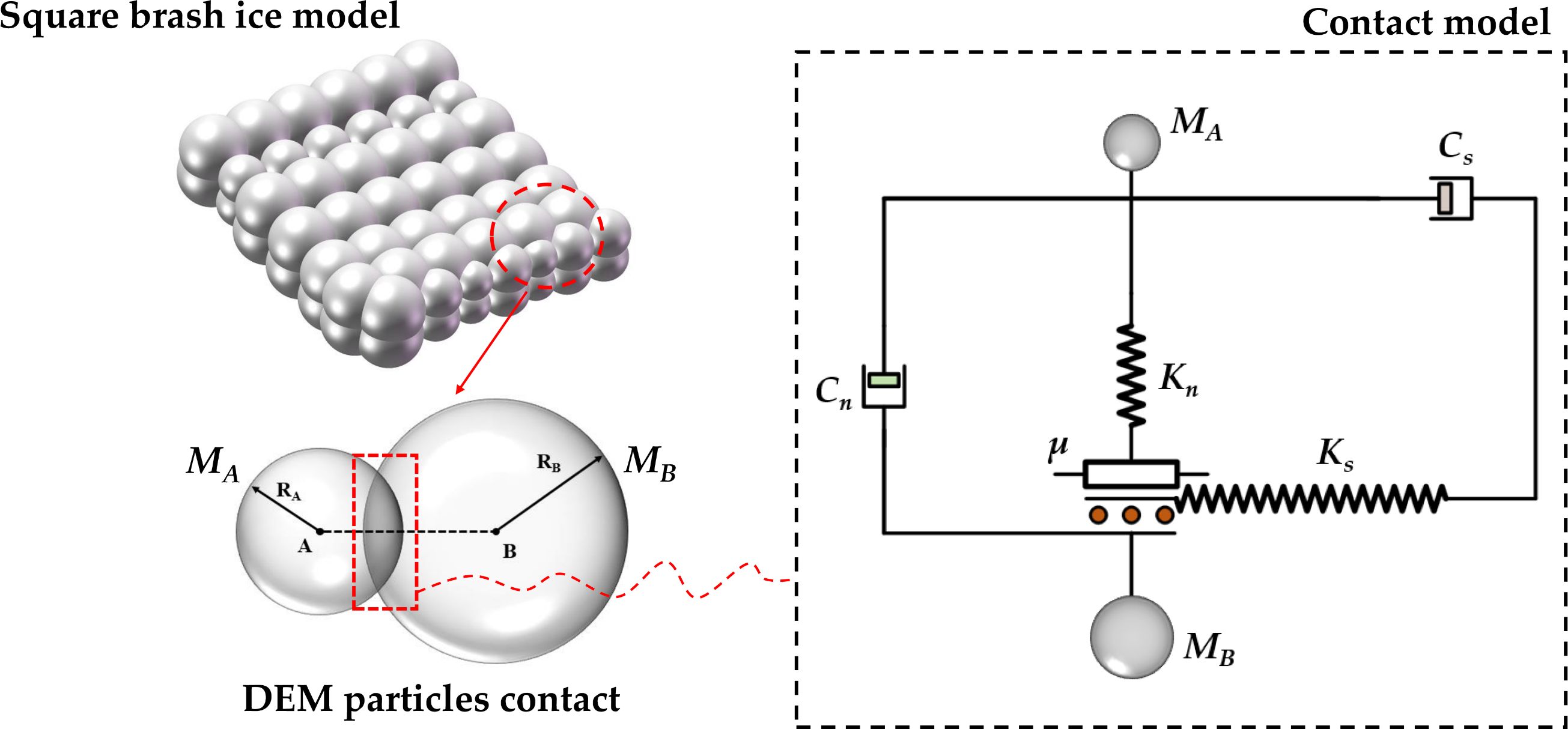
Figure 1. The contact model between DEM particles of brash ice.

$\begin{array}{ll}{\sigma }_{max}=\frac{-F_n}{A}+\frac{\left|M_S\right|}{I}{R}_c& (3)\end{array}$

$\begin{array}{ll}{\tau }_{max}=\frac{\left|F_S\right|}{A}+\frac{\left|M_n\right|}{J}{R}_c& (4)\end{array}$

Where A is the cross-sectional area of the cohesive disc model; R_c is the radius of the cohesive model; J is the polar moment of inertia of the cohesive model, J=0.5πR_c²; I is the moment of inertia of the cohesive model, I=0.25πR_c²; F_n and F_s represent the normal contact force and the tangential contact force between particles, respectively; M_n and M_s represent the normal and tangential moments between particles, respectively.

According to the tension-shear zone fracture criterion, when σ_max > σ_t, cohesive failure occurs between particles due to tensile fracture; when τ_max > τ_s, cohesive failure occurs between particles due to shear fracture. The tensile failure strength σ_t and shear failure strength τ_s are shown in Equations 5 and 6, respectively:

$\begin{array}{ll}{\sigma }^t={\sigma }_b^n& (5)\end{array}$

$\begin{array}{ll}{\tau }^S={\sigma }_b^S+{\mu }_b{\sigma }_{max}& (6)\end{array}$

Where σ_bⁿ and σ_b^s represent the normal bond strength and shear bond strength, respectively; μ_b denotes the internal friction coefficient, μ_b=0.23(σ_c-σ_f)-0.5. σ_c and σ_f represent the compressive and flexural strength of sea ice, which can be determined as follows:

$\begin{array}{ll}{\sigma }_c=3.5\times (1.77-1.81e^{-\frac{L/D}{4.78}}){\sigma }_b& (7)\end{array}$

$\begin{array}{ll}{\sigma }_f=(1.77-1.81e^{-\frac{L/D}{4.78}}){\sigma }_b& (8)\end{array}$

In Equations 7 and 8, L and D represent the thickness and number of layers of the constructed sea ice, respectively.

When the interaction between sea ice occurs, the relationship between force and displacement needs to be defined through a contact model. The contact forces between sea ice discrete elements include the normal contact force F_n and the tangential contact force F_s. According to the Hertz-Mindlin contact theory (Zhang et al., 2022), F_n can be expressed as:

$\begin{array}{ll}{F}_n=F_e+F_V& (9)\end{array}$

In Equation 9, F_e is the elastic force between particle units, F_e=K_n·x_n; F_v is the damping force between particle units, F_v=-C_n·v_n. x_n and v_n represent the overlap volume and normal relative velocity between elements. K_n is the equivalent stiffness between two contacting particle units; C_n represents the normal damping coefficient between the two contacting units, defined in Equation 10.

$\begin{array}{ll}{C}_n={\xi }_n\sqrt{2M{K}_n}& (10)\end{array}$

Where M is the equivalent mass of two-particle units. The damping ratio ξ_n can be obtained by Equation 11:

$\begin{array}{ll}{\xi }_n=\frac{-ln{e}_i}{\sqrt{{\pi }^2+{ln}^2{e}_i}}& (11)\end{array}$

Here e_i is the coefficient of resilience.

The tangential contact force F_s between elements can be determined based on Coulomb’s friction law, as shown in Equation 12.

$\begin{array}{ll}{F}_s=min(|K_s{x}_s-C_s{v}_s|,|\mu F_n|)& (12)\end{array}$

Where x_s and v_s represent the tangential displacement increments and tangential relative velocity between the two contacting units, respectively; K_s is the tangential stiffness, K_s=α·K_n; C_s is the tangential damping coefficient, C_s=β·C_n.

Finally, the contact time T_bc from collision to separation between two units is shown in Equation 13:

$\begin{array}{ll}{T}_{bc}=\frac{\pi }{\sqrt{\frac{2K_n}{M}(1-{\xi }_n^2)}}& (13)\end{array}$

2.3 Particle-fluid interaction

In the fluid domain, DEM particles representing brash ice are mainly subjected to buoyancy, drag resistance, lift force, and additional mass forces. Buoyancy can be obtained by calculating the volume of particles underwater using the Catto algorithm (Yang, 2022). The drag resistance is calculated according to Morrison's formula (Equation 14):

$\begin{array}{ll}{F}_{drag}=-0.5C_d{\text{ρ}}_f{A}_{proj}{U}_{rel}\left|U_{rel}\right|& (14)\end{array}$

Where C_d is the drag coefficient and ρ_f is the fluid density. U_rel and A_proj are the relative velocity of the particle to the fluid and the projected area of the particle immersed along the direction of relative velocity, respectively.

The lift force exerted by the fluid on the particle can be estimated as Equation 15.

$\begin{array}{ll}{F}_{lift}=1.515D^2{(\text{ρ}\mu )}^{0.5}\left|\frac{\partial v}{\partial y}\right|U_{real}& (15)\end{array}$

Where D is the particle diameter and ρ is the particle density. μ and v represent the dynamic viscosity and fluid velocity.

The expression of additional mass forces on the particle (Equation 16):

$\begin{array}{ll}{F}_a=C_{vm}{\text{ρ}}_w{V}_p(\frac{d{U}_{real}}{dt}-\frac{d{v}_p}{dt})& (16)\end{array}$

Where C_vm is the additional mass factor, V_p is the particle volume and v_p is the particle velocity.

3 Numerical brash ice tank and ice model test

3.1 Numerical brash ice tank

The numerical brash ice tank is constructed using Star CCM + software. Eulerian multiphase flow and the DEM are employed to simulate fluid motion and mixed brash ice movement, respectively. The computational domain size (length × width × height) is set as 800m × 380m × 300m, as shown in Figure 2. Two level ice zones are established at the draft height of the ship, with the remaining central area designated as the numerical brash ice channel. An ice injector is installed at the end of the numerical channel to generate a mixed brash ice model. Following the recommendations of the International Towing Tank Conference (ITTC) on ice tank tests (Recommended Procedures and Guidelines: Section 7.5–02-04 for Ice Testing, 2014), the width of the numerical ice channel is twice the width of the ship. When calculating ice loads using DEM, it is sufficient to model the hull structure of the ship, considering the ship as a rigid body. It is assumed that when the ship collides with brash ice, the ice will not break into smaller pieces.

Figure 2

Figure 2. The numerical brash ice tank.

3.2 Brash ice model tests

To investigate ship-ice interaction and subsequently verify the effectiveness of the numerical brash ice tank, the brash ice model test at Hamburg Ship Model Basin (HSVA) is introduced (IO 509/12; Brash Ice Tests for a Panmax Bulker with Ice Class 1B, 2013). The ice model test utilized an Ice Class tanker as the research subject, with the full-scale dimensions (length overall × molded breadth × molded depth × draft) of 250m × 44m × 21.2m × 15m. The scale ratio between the ship model and the actual ship is 1:30.66. Figure 3 displays the bow and stern of the ice-class test ship model.

Figure 3

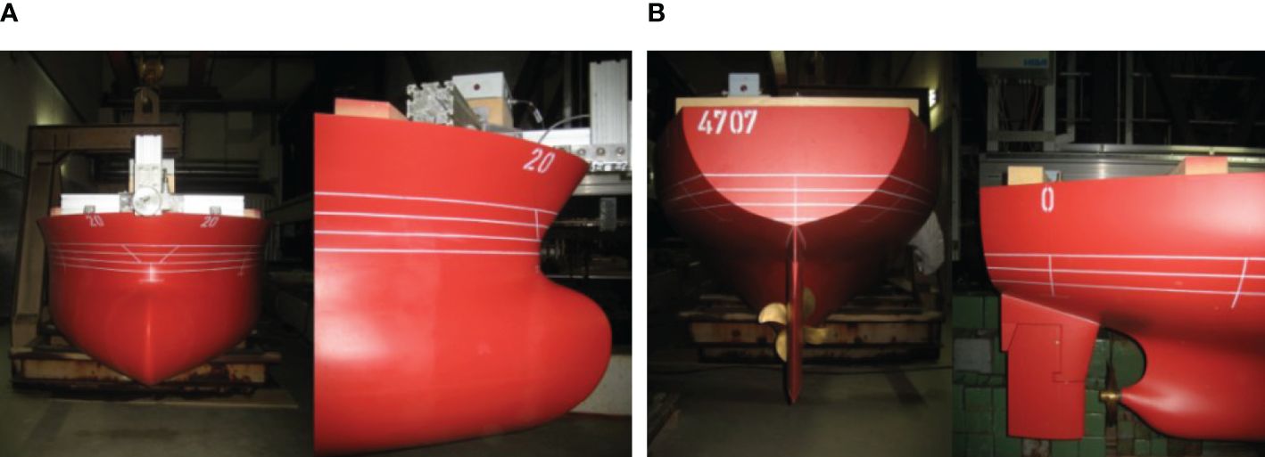
Figure 3. The Ice Class tanker model: (A) Bow; (B) Stern.

The most complex and critical step in the ice model test is the generation of the brash ice channel. According to HSVA’s brash ice model test preparation procedure, it is necessary to first prepare a parental level ice sheet with the required thickness in the open water channel. Once the thickness of level ice meets the requirements, the environmental temperature is gradually increased. When the ambient temperature stabilizes at around -2°C, the ice cutter is used to make a straight-line cut on the level ice sheet, creating an area equal to twice the ship’s width. This area serves as the pre-treatment zone for the brash ice channel. Subsequently, the ice bars in the pre-treatment zone are shattered into relatively smaller fragments using a special ice chisel, forming a brash ice channel. Supplementary Figure S1 illustrates the process of preparing brash ice and the finished brash ice channel.

Ice concentration refers to the coverage area of sea ice within a specific region, which is one of the critical factors influencing the results of ice load. In ice tank tests, photography or video equipment is typically used to capture sea ice distribution in the ice tank from above. Subsequently, image analysis techniques are used to determine the coverage area of the ice. By iteratively capturing and analyzing images, the ice concentration is ultimately adjusted to meet the experimental requirements.

In the brash ice tank test, the brash ice remained stationary, and the ship-ice collision is carried out through towed propulsion, with the ship speed set at 3 knots. Test conditions are divided based on ice thickness and draft. Ice load measurement sensors are installed on the bow deck of the ship, and the ship model is towed through the entire brash ice channel under each test condition. Supplementary Figure S2 depicts the ship model during the experiment.

4 Comparison between the ice model test and numerical simulation

In this paper, the numerical simulation of ship-ice collision is carried out using a 120m Ice Class ship as an example. The brash ice simulating the navigational channel is kept stationary, while the cargo ship travels at a certain rated power, thereby simulating the collision process between brash ice and the ship. Supplementary Table S1 presents the main dimensions of the ice-class ship and the ice parameters used in the numerical simulation.

4.1 Sea ice DE model

The complexity of the brash ice DE model is not only related to the contact model between particles but also to the particle shape. Compared to cylindrical and polyhedral particles, the contact determination algorithm for spherical particles is relatively simple (Zhu and Ji, 2022). Due to the numerous working conditions involved in the numerical calculation of ice loads and fatigue analysis later in the paper, from the perspective of computational cost and efficiency, spherical particles are chosen as the basic unit of the DE model to simulate brash ice. Unlike previous studies focusing on a single shape of brash ice (Li et al., 2013), to more reasonably compare numerical simulation results with experimental results, this paper refers to the ice shape in the HSVA’s ice model test, and uses the composite particle filling method of STAR CCM + software to generate multi-shaped brash ice. Supplementary Figure S3 presents the DE model of brash ice established by referring to the shape of brash ice in the HSVA’s ice tank.

4.2 Comparison of ship-ice collision phenomena between brash ice model test and numerical simulations

To validate the rationality of the numerical ice tank, the ice particle behavior in numerical simulations during the ship-ice collision at 90% sea ice concentration is compared with experimental results at the HSVA, as shown in Figure 4. In numerical simulations, different sea ice concentrations can be achieved using the inverse method, as outlined in the following steps: First, based on the total surface area of the numerical ice tank, calculate the ice-covered area corresponding to different ice concentrations. Then, determine the total number of DEM particles required for the entire simulation period according to the ice-covered area. Finally, based on the calculated total number of particles, infer in reverse the number of particles that need to be injected per unit time (each step) during the simulation.

Figure 4

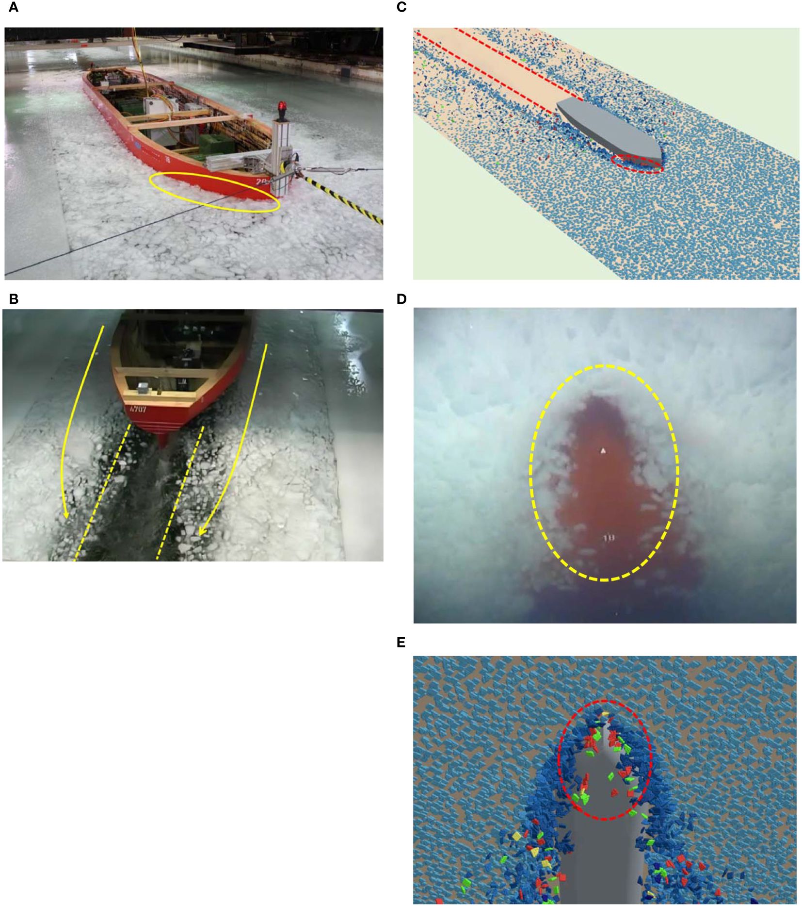
Figure 4. Numerical and experimental results of ship-ice collisions at 90% ice concentration. (A) Collision, Accumulation, and Extrusion of brash ice at the bow. (B) Brash ice channel behind the hull in the ice model test. (C) Ship-ice collision state in the numerical ice tank. (D) Brash ice on the bottom of the ship in the ice model test. (E) Brash ice on the bottom of the ship in the numerical ice tank.

From Figures 4A–C, it can be observed that when the ship comes into contact with brash ice, continuous collisions, accumulation, and extrusion occur between them. These actions constitute the main reasons for the generation of ice resistance. In addition, when the ship sails forward, brash ice at the bow is continuously pushed aside to both sides of the hull, causing friction and compression on the surfaces of both sides. A clear channel without brash ice, approximately equal to the ship’s width, is formed in the wake behind the ship. Observing Figures 4D, E, it becomes obvious that during the collision between the ship and brash ice, some pieces of ice are pressed into the bottom of the ship. The numerical simulation results of ship-ice collision are in basic agreement with the observations from the ice tank test, indicating that the injected numerical brash ice field used in this paper can effectively simulate the interaction during ship-ice collisions.

4.3 Calculation of ice load

For the issue related to ship-ice collision, the bow of the ship serves as the primary loading area. To minimize computational costs for subsequent fatigue assessments, the high-pressure area on the bow of the target vessel is chosen as the output location for ice loads. The overall time history curve of ice loads is obtained by synthesizing the time history curves in the x, y, and z directions. Supplementary Figure S4 illustrates the ship-ice collision process for the target vessel, with a speed of 3 knots, ice thickness of 0.7 meters, and a brash ice concentration of 90%. Based on Dr. Zhao’s research (Zhao, 2021), to maintain the accuracy of fatigue damage calculations, the time for time-domain analysis is typically set to a minimum of 5 minutes. Therefore, we have also set the simulation time for ship-ice collision to 300 seconds. The time history of the ice load on the target vessel is depicted in Figure 5. It can be observed that the time history of ice loads exhibits significant fluctuations during the interaction between the ship and the brash ice. When the ship’s bow first contacts the brash ice, an instantaneous loading process occurs, causing the ice load to suddenly increase. As the ship continues to advance, the brash ice is gradually pushed aside to both sides of the hull, resulting in a sharp decrease in ice load. After a certain period, the brash ice accumulates at the bow, causing the ice load to reach a higher value again. Once the accumulation reaches a certain level, the brash ice overturns, and the accumulated ice gradually clears to the sides of the ship, causing the ice load to decrease significantly.

Figure 5

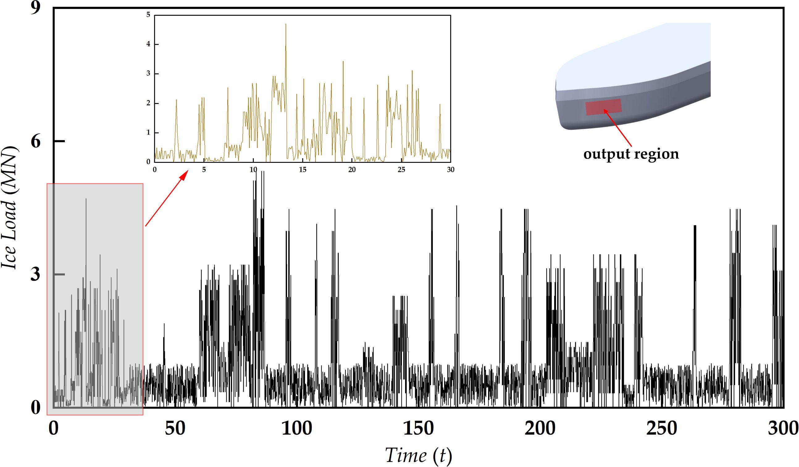
Figure 5. The time history of ice loads at a speed of 3 kn.

4.4 Verification of ice load

Because of discrepancies between parameters and structure for the numerical model and experimental model caused by issues related to later fatigue studies, it is not possible to directly compare numerical values of ice loads. To validate the reliability of the time histories of ice loads calculated based on the CFD-DEM coupling method, the mean and amplitude of the ice load are verified separately.

Firstly, taking the condition of 90% sea ice density as an example, the mean of the ice load is validated with reference to the DUBROVIN empirical formula for brash ice area ship-ice collision. According to the DUBROVIN formula, the ice load L_ice at different speeds can be expressed as:

$\begin{array}{ll}{L}_{ice}=p_1{C}_A+p_2\phi F{r}^n& (17)\end{array}$

In Equation 17, p₁ and p₂ are empirical coefficients related to the channel width, with values of 0.12 and 3, respectively. n and F_r respectively represent the power coefficient and Froude number. C_A and φ are calculated coefficients related to the main dimensions of the ship and the ice body, which can be obtained by Equations 18 and 19.

$\begin{array}{ll}{C}_A=\frac{1}{4}{B}^2\sqrt{r{h}_i}{\rho }_i(1+2\frac{L}{B}{\mu }_{s-i}{\alpha }_H)& (18)\end{array}$

$\begin{array}{ll}\phi =r{h}_i{\rho }_{i}B[{\mu }_{s-i}+tan{\alpha }_0({\alpha }_H+\frac{L}{B}tan{\alpha }_0)]& (19)\end{array}$

Here h_i represents the thickness of the brash ice. α_H is the wedge coefficient of the bow of the ship. α₀ is half the angle of incidence of the waterline.

Figure 6 illustrates the comparison between the mean values of ice load histories calculated by the CFD-DEM method at different speeds and the results calculated by the DUBROVIN formula. Generally, the trends of both methods are consistent. At lower speeds, the CFD-DEM method tends to yield smaller results compared to the DUBROVIN formula, but at higher speeds, the discrepancy diminishes. This discrepancy arises from the assumption in numerical calculations that the DE model of brash ice cannot be further broken, limiting the generation of additional ice fragments. This difference is more pronounced at lower speeds. However, at higher speeds, the instantaneous contact force during ship-ice collision is relatively large, which to some extent mitigates the impact of this assumption. From the error analysis perspective, in the low-speed range (3–7 kn), the discrepancy between numerical results and empirical results is significant, with an average error of 42.2%. In the high-speed range (8-12 kn), this error decreases, with an average error of only 9.4%. This pattern of variation is consistent with the findings of previous studies (Yang et al., 2020; Wang et al., 2023).

Figure 6

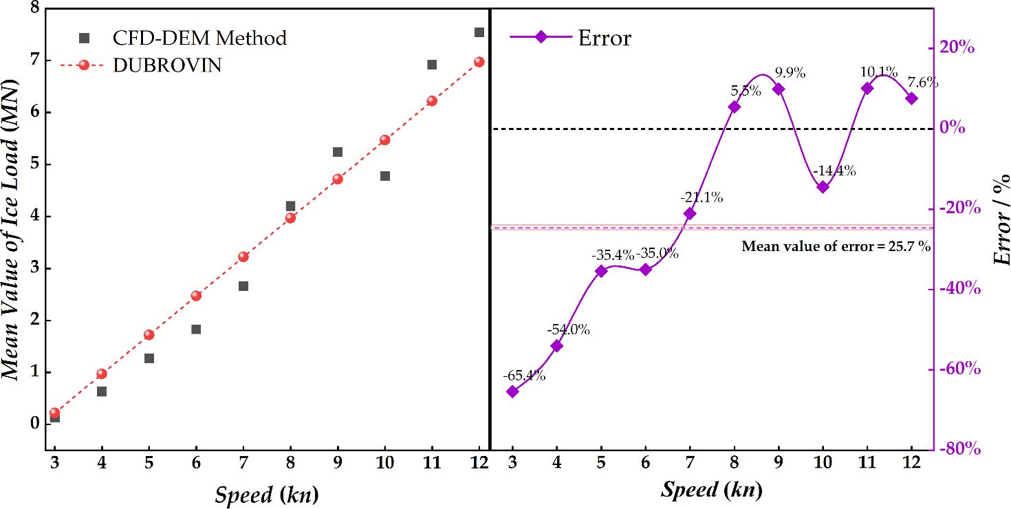
Figure 6. Comparison of results of the CFD-DEM method with the DUBROVIN Formula.

Based on the measured ice load data of the KV Svalbard ship (Leira et al., 2009) and subsequent studies (He et al., 2023), it is indicated that the distribution of ice load amplitudes most likely follows a lognormal distribution and a Weibull distribution. The calculated ice load amplitudes are statistically analyzed, and their probability density function (PDF) is depicted in Figure 7. It can be observed that the PDF of ice load amplitudes generally follows a two-parameter Weibull distribution (k = 3.6360, r = 98.2960) and a log-normal distribution (λ_ln = 1.954, σ_ln = 0.3).

Figure 7

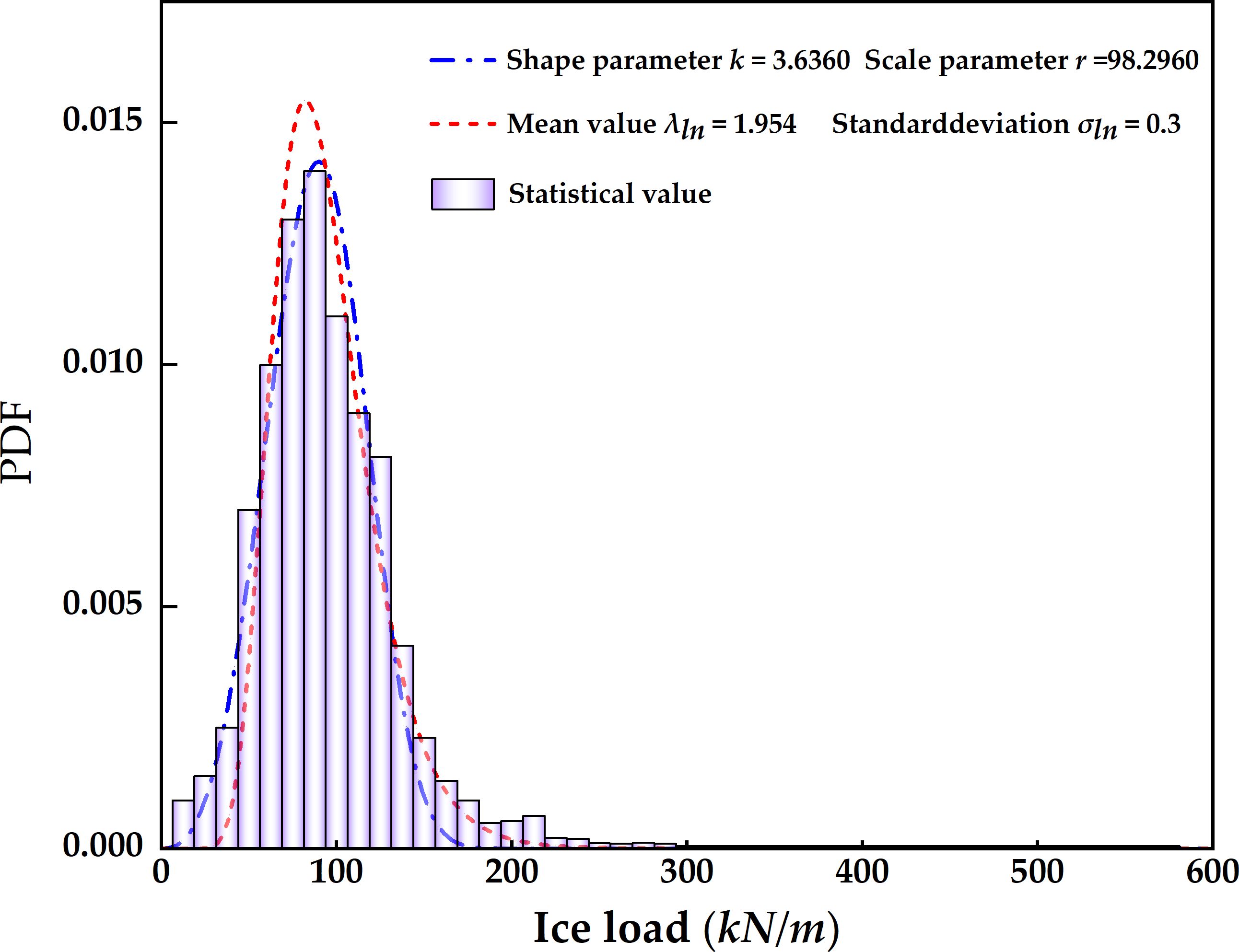
Figure 7. PDF of ice load amplitude.

As mentioned, we can conclude that the ice load time history computed by the CFD-DEM method exhibits a certain level of reliability and can be utilized for subsequent fatigue damage analysis.

5 Calculation of hot spot stress response for ice-induced fatigue

5.1 Working conditions

In fatigue analysis, reasonable division of working conditions is a critical factor influencing the results of fatigue assessment (Putra et al., 2023). The transportation route for the target vessel is the East Siberian Route, covering a total distance of 1014.24 nautical miles. The vessel undertakes this journey 10 times per year, and its designed lifespan is 25 years, resulting in a total mileage of 253,560 nautical miles during its operational life. The fatigue damage of polar ship structures is significantly influenced by ice loads, where ice thickness, sea ice concentration, and speed are the key factors determining the magnitude of these loads. Research indicates that ice-induced fatigue damage is primarily caused by sea ice with a thickness exceeding 0.7m. Combining the probability density distribution curve of ice thickness in literature (Chang, 2022) with the conditions of the target vessel’s navigation area, an ice thickness of 0.7m is selected. Sailing speed and sea ice concentration are also critical factors influencing the structural fatigue damage analysis of ships in brash ice fields. In this study, 12 fatigue sub-conditions are established, each with a probability of occurrence of 1/12, using sailing speed and sea ice concentration as variables, as detailed in Table 1. Assigning equal probability to each working condition is necessary for subsequent sections that compare the influence of different sailing speeds and sea ice concentrations on fatigue responses. It ensures that sea ice concentrations and speeds have the same total duration over the entire voyage life.

Table 1

Table 1. Ice-induced fatigue assessment conditions.

5.2 Calculation of hot spot stress response

According to the research findings of previous studies (Han et al., 2023), significant ice-induced fatigue damage is often found in the side shell near the bow waterline during ship-ice collisions. Additionally, when the ship encounters ice loads, it generates upward compression forces and vertical bending moments. Therefore, fatigue failure is also prone to occur at locations such as the hull deck and hatch corners. This paper, referring to existing literature (Jeon and Kim, 2022) and the China Classification Society (CCS) rules, has selected four specific regions of the cargo ship as hot spots for fatigue assessment, as outlined in Supplementary Table S2.

The hot spot stress is calculated by fine mesh finite element (FE) analysis, with the surface extrapolation method chosen for interpolation. In FE modelling, shell elements are used to simulate plate, and beam elements are used to simulate framing. The size of each FE mesh corresponds to the size of the panel. The whole FE model primarily consists of quadrilateral elements, with triangular elements used for transitions at complex structural connections. To more accurately predict the fatigue damage of the hull structure, the material characteristics are assumed to be isotropic hardening. Mesh refinement follows the CCS specification principle. The time history of ice loads is applied to the FE model for dynamic response analysis, yielding the stress time history at the hot spot position. Figure 8 displays both the FE model of the target ship and the fine mesh FE model at the hot spot locations.

Figure 8

Figure 8. FE model of the target ship and fatigue hot spots.

Figure 9 illustrates the stress time histories for hot spot 4 under a consistent sea ice concentration (50%) but varying speeds, Figure 10 displays the fluctuation in the mean stress of hot spot 4 with the speed across different sea ice concentrations. We can see that within the same time frame (0-300 seconds), as the ship speed increases, more stress peaks are likely to occur. This is because the faster the ship speed, the higher the collision frequency between the brash ice and the bow, the longer the continuous collision time, and the more obvious the accumulation phenomenon between the brash ice. Although the mean stress from 0-300s increases with the ship’s speed, the trend of stress increase gradually slows down, in some cases, decreases with further speed increments. This is due to the hull’s wave-making effect becoming prominent at higher speeds, exerting a repulsion influence on the surrounding brash ice. Consequently, the brash ice moves away from the hull surface, diminishing the probability of contact and collision between the brash ice and the hull.

Figure 9

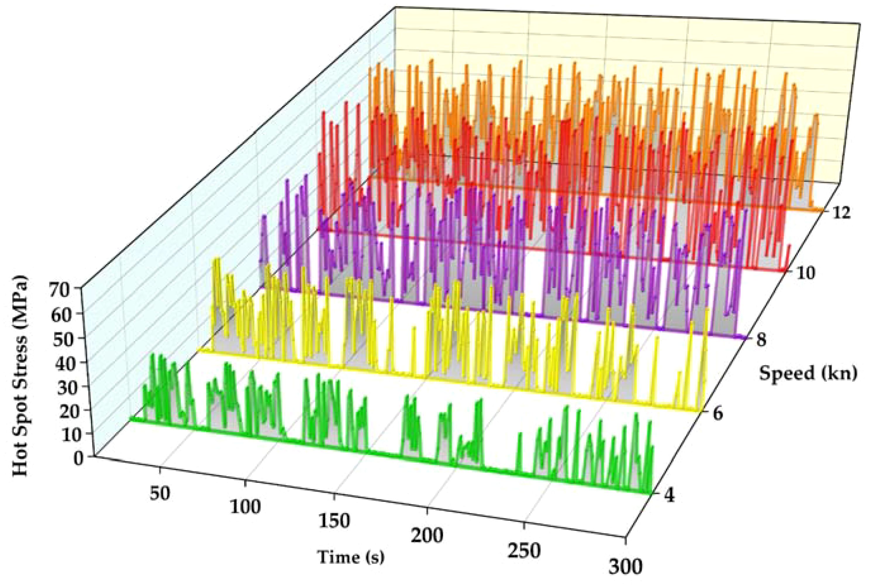
Figure 9. The hotspot stress time histories under different speeds.

Figure 10

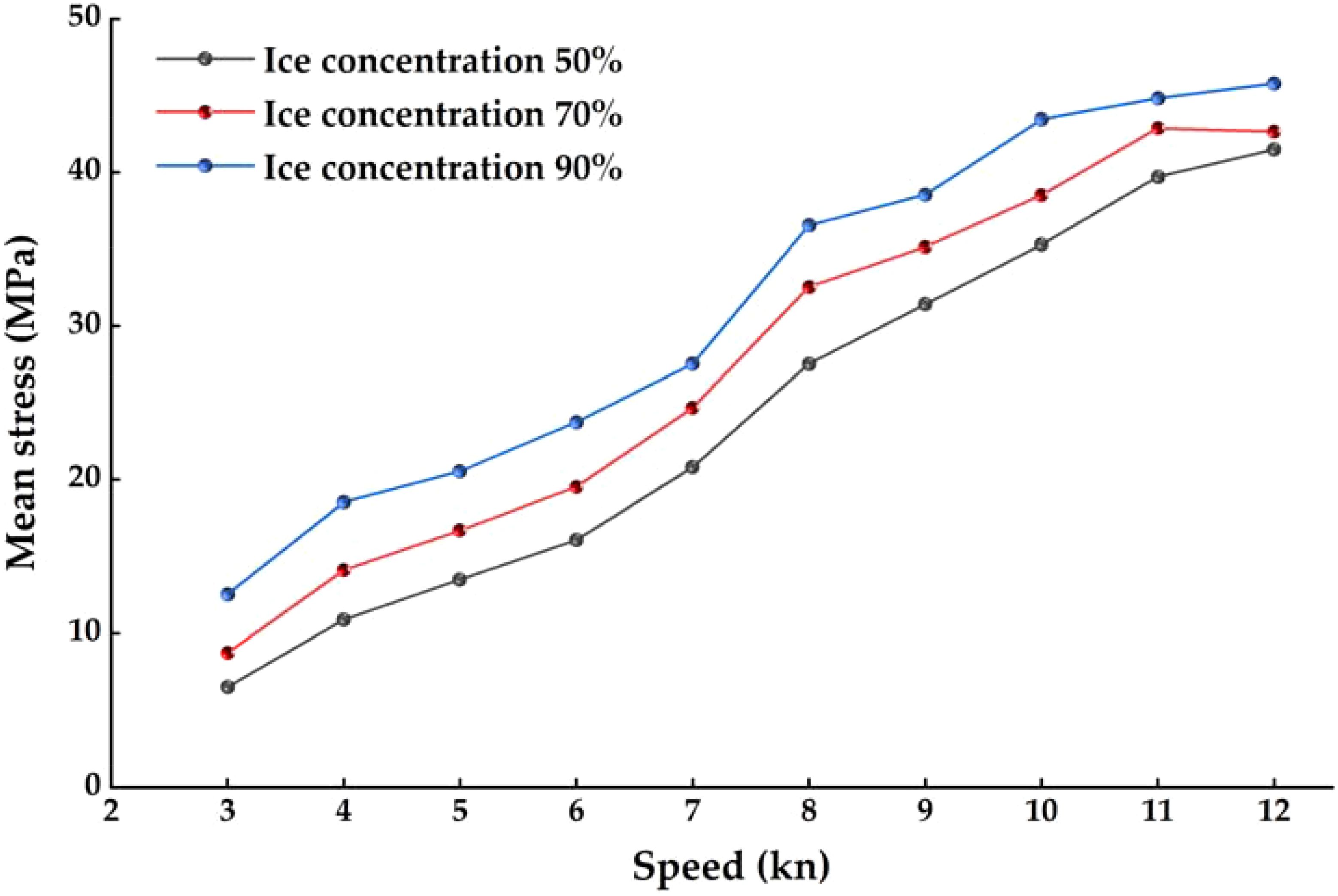
Figure 10. The variation of the mean stress with the speed.

6 Results and discussion

6.1 Simulation framework of the coupled CFD-DEM-FEM

Supplementary Figure S5 depicts the fatigue assessment framework for polar ships using the CFD-DEM-FEM coupling method. The process begins with the calculation of the load interaction between the ship and the brash ice by Star CCM+ software. Next, using MSC. Patran, the FE model of the ship is established and the mesh is refined at the evaluated hot spots. The ice load time history is applied to the FE model to obtain the stress time history of the evaluated hot spots. The stress time history is statistically analyzed to obtain the stress levels of the hot spots using the rain-flow counting method. Finally, the fatigue damage of the hot spots is determined using the S-N curve method, based on the linear cumulative damage criterion.

6.2 Fatigue damage calculation method of ice-going ships

Taking any hot spot to be evaluated as an example, firstly, stress levels of the hot spot within the rain flow counting period t₁ under fatigue subcondition 1 are counted. n_ij denotes the number of stress cycles corresponding to the i-level stress amplitude and the j-level stress mean. The fatigue damage D_t1-_ij of the hot spot within the rain flow counting period t₁ can be expressed as:

$\begin{array}{ll}{D}_{t1,ij}=\frac{n_{ij}}{N_{ij}}& (20)\end{array}$

In Equation 20, N_ij represents the stress cycle count corresponding to that stress level in the S-N curve.

Based on the Palmgren-Miner linear cumulative damage theory, the fatigue damage D_t1 generated by all stress levels under the fatigue sub-condition 1 within the rain flow counting period t₁ can be calculated by Equation 21.

$\begin{array}{ll}{D}_{t1}={\displaystyle \sum _{i=1}^m{\displaystyle \sum _{j=1}^n{D}_{t1-ij}}}={\displaystyle \sum _{i=1}^m{\displaystyle \sum _{j=1}^n\frac{n_{ij}}{N_{ij}}}}& (21)\end{array}$

However, it must be pointed out that the sailing time of the ship cannot be limited solely to the rain-flow counting period t₁. If the total sailing distance of the ship under the fatigue subcondition 1 is denoted as S₁, and the sailing distance of ships within the rain flow counting period t₁ is denoted as L₁, then the fatigue damage D₁ of the fatigue subcondition 1 can be expressed using Equation 22.

$\begin{array}{ll}{D}_1={\displaystyle \sum _{i=1}^m{\displaystyle \sum _{j=1}^n\frac{S_1}{L_1}{D}_{t1-ij}}}=\frac{S_1}{L_1}{\displaystyle \sum _{i=1}^m{\displaystyle \sum _{j=1}^n\frac{n_{ij}}{N_{ij}}}}& (22)\end{array}$

The fatigue damage D of the hot spots under all fatigue sub-conditions (assuming K sub-conditions) can be obtained by Equation 23:

$\begin{array}{ll}\begin{array}{c}D=D_1+D_2+\dots +D_K\hfill \\ =\frac{S_1}{L_1}{\displaystyle \sum _{i=1}^m{\displaystyle \sum _{j=1}^n{D}_{t1-ij}}}+\frac{S_2}{L_2}{\displaystyle \sum _{i=1}^m{\displaystyle \sum _{j=1}^n{D}_{t2-ij}}}+\dots \frac{S_K}{L_K}{\displaystyle \sum _{i=1}^m{\displaystyle \sum _{j=1}^n{D}_{tK-ij}}}\hfill \end{array}& (23)\end{array}$

6.3 Ice-induced fatigue damage assessment of hot spots

As mentioned earlier, to calculate the fatigue damage of hot spots on ice-going ships, the initial step involves obtaining the stress level of the stress time history. This study employs the improved rain-flow counting method (Gao et al., 2023) to statistically analyze the stress time histories calculated in Chapter 4 under various working conditions, ultimately obtaining the stress level of the hot spot. It is important to note that the stress ratio R of stress cycles obtained through rain-flow counting for stress time histories is not equal to -1. This means that directly applying the Palmgren-Miner cumulative damage criterion for fatigue damage calculation is impractical. Therefore, this paper utilizes the Goodman correction method to perform average stress corrections for each stress cycle. The expression of Goodman correction (Equation 24):

$\begin{array}{ll}\frac{S_a}{S_c}+\frac{S_m}{S_u}=1& (24)\end{array}$

Where S_a and S_m represent the stress amplitude and the mean stress in a given stress cycle, respectively. S_u is the ultimate strength of the material. S_c is the stress amplitude corresponding to the stress ratio R=-1 after Goodman correction.

The statistical results are presented in Supplementary Figure S6 (using condition 5 as an example).

When the time domain method based on the S-N curve is used to calculate the fatigue damage, the selection of a suitable S-N curve is crucial. Considering the unique low-temperature conditions in ice-prone areas, relying on a standard temperature S-N curve for calculating fatigue damage of hot spots can result in substantial errors. In this paper, the low-temperature S-N curve obtained by the experiment in Reference (Wang YT. et al., 2021) is used to calculate the fatigue damage of hot spots. Table 2 lists the ice-induced fatigue damage of hot spots under various working conditions.

Table 2

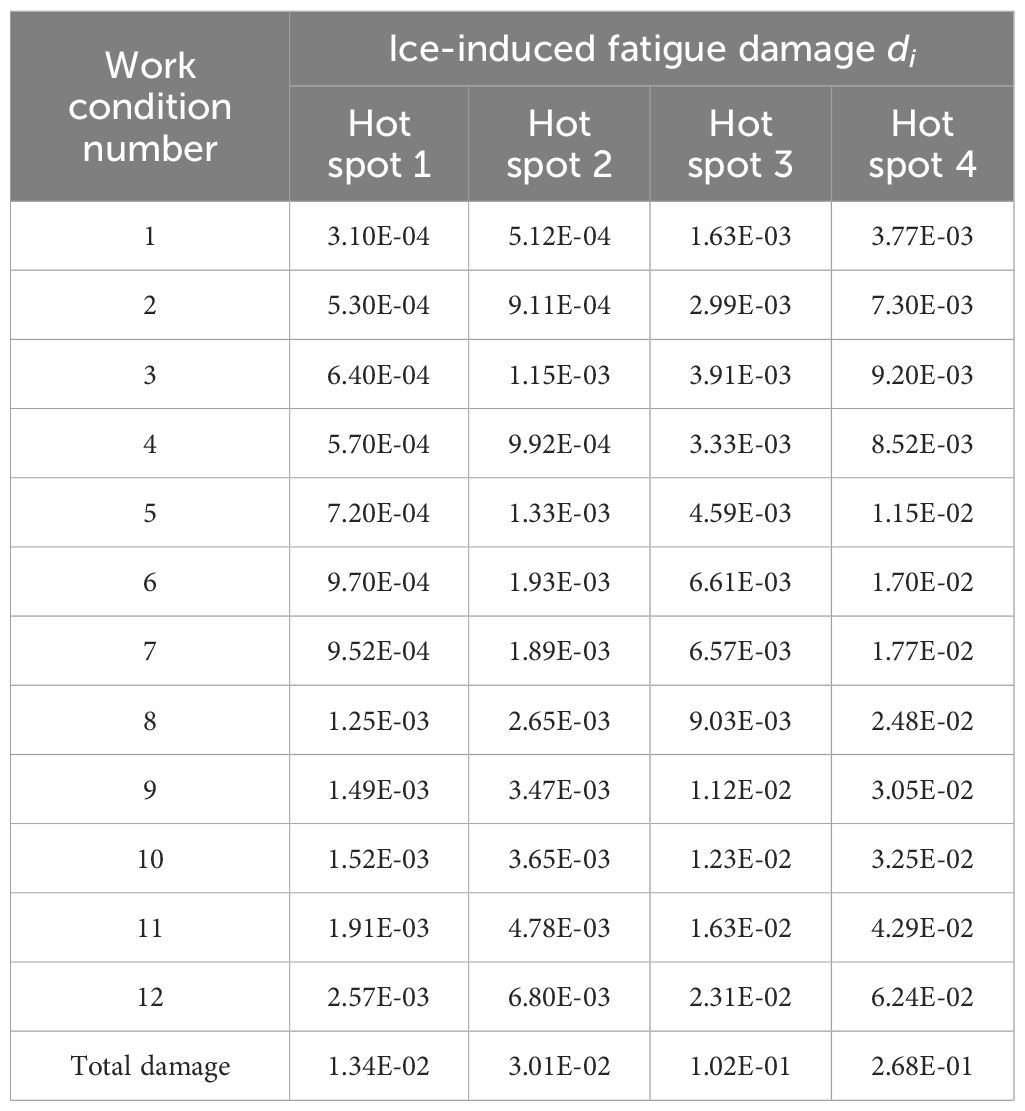
Table 2. Ice-induced fatigue damage of hot spots from different conditions.

From Table 2, it is evident that the fatigue damage of hot spot 1 is the consistently smallest under all working conditions. This is attributed to the location of hot spot 1 in the hatch corner, farthest from the bow-brash ice collision area. The fatigue damage of hot spot 1 serves as the benchmark, and the damage error rate is defined as e_i = (d_i-d₁)/d₁ × 100%. Figure 11 illustrates the error rate of fatigue damage for each hot spot compared to the fatigue damage of hot spot 1. Hot spot 4, situated in the direct collision area between the bow side and sea ice, exhibits the largest fatigue damage, averaging 1896% higher than that of hot spot 1. Hotspots 2 and 3 show an average increase in fatigue damage of 124% and 656%, respectively, compared to Hotspot 1. Although hot spot 2 and 3 are close to the bow-ice collision area, hot spot 3 is near the waterline, while hot spot 2 is farther from the waterline. From the ice tank test and numerical simulation, it is observed that when brash ice collides with the hull, the ice accumulates and slides near the waterline. Consequently, significant alternating stresses occur in this region. This explains the higher fatigue damage in hot spot 3.

Figure 11

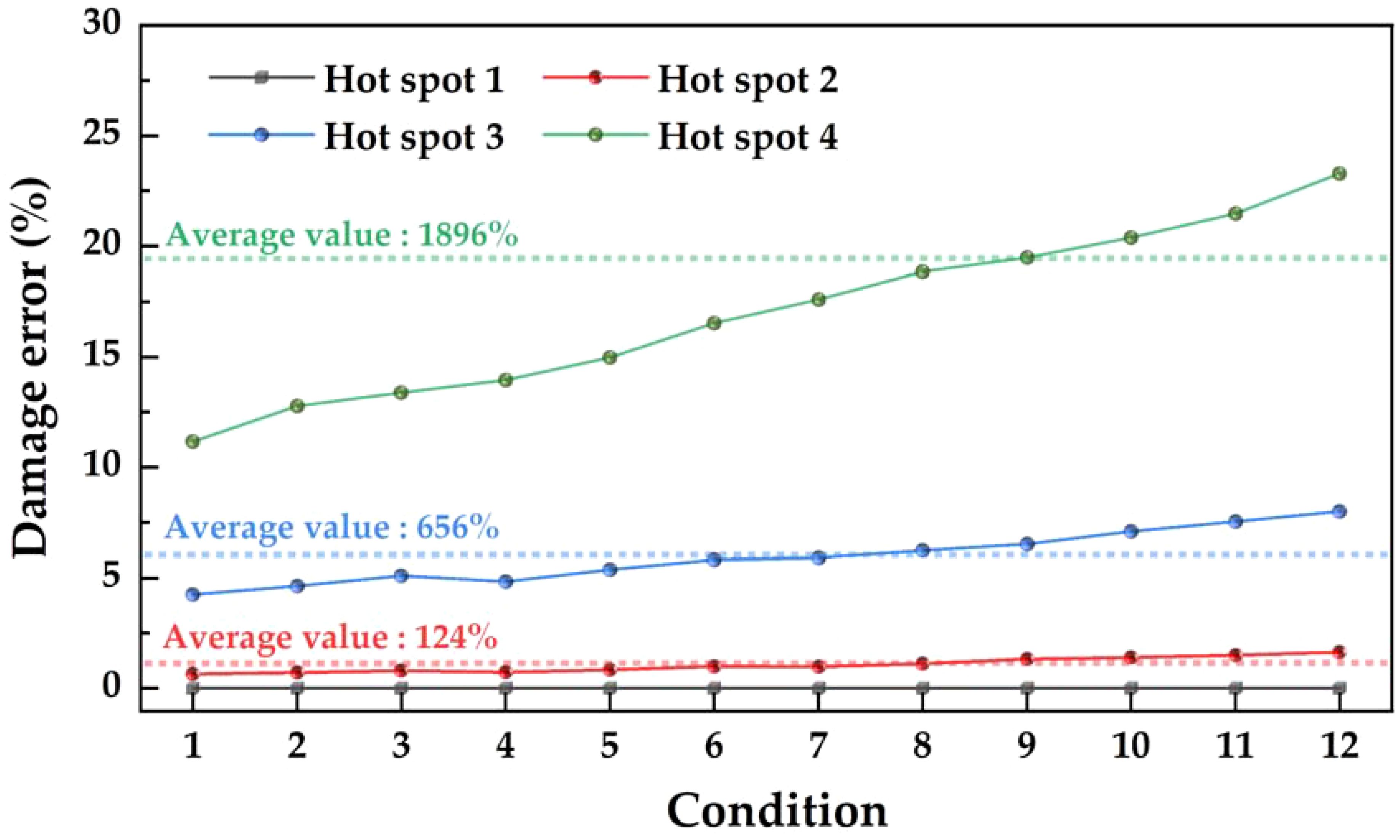
Figure 11. The damage error rate for each hot spot compared to hot spot 1.

Finally, according to the Lloyd’s Register specification, the fatigue damage for polar navigation ships should be less than 0.5. It is evident that the fatigue damage at the four typical locations of the ice-class cargo ship all meets the design requirements.

6.4 Verification of fatigue assessment results

To validate the rationality of the proposed ice-induced fatigue assessment method in this paper, the LR FAD-ICE was used to calculate the fatigue damage for the four hotspots discussed in the article. Figure 12 illustrates the comparison between the proposed method in this paper and the LR method. The fatigue damage calculated by the LR method is about 1.85 times higher than that of the DEM-FEM method, and the ratio of the hot spot position with the larger fatigue damage is larger. This difference arises because the LR method is simplified. Firstly, it calculates the hot spot stress induced by ice loads using beam theory. Secondly, in the LR method, the distribution of ice load amplitudes and the number of ship-ice collisions are obtained through empirical formulas, neglecting the influence of sea ice concentration and the relative velocity between the ship and ice. These factors contribute to the conservative nature of LR assessment results. It is crucial to emphasize that the comparison with the LR method serves as validation for the rationality of the proposed method rather than a strict accuracy test.

Figure 12

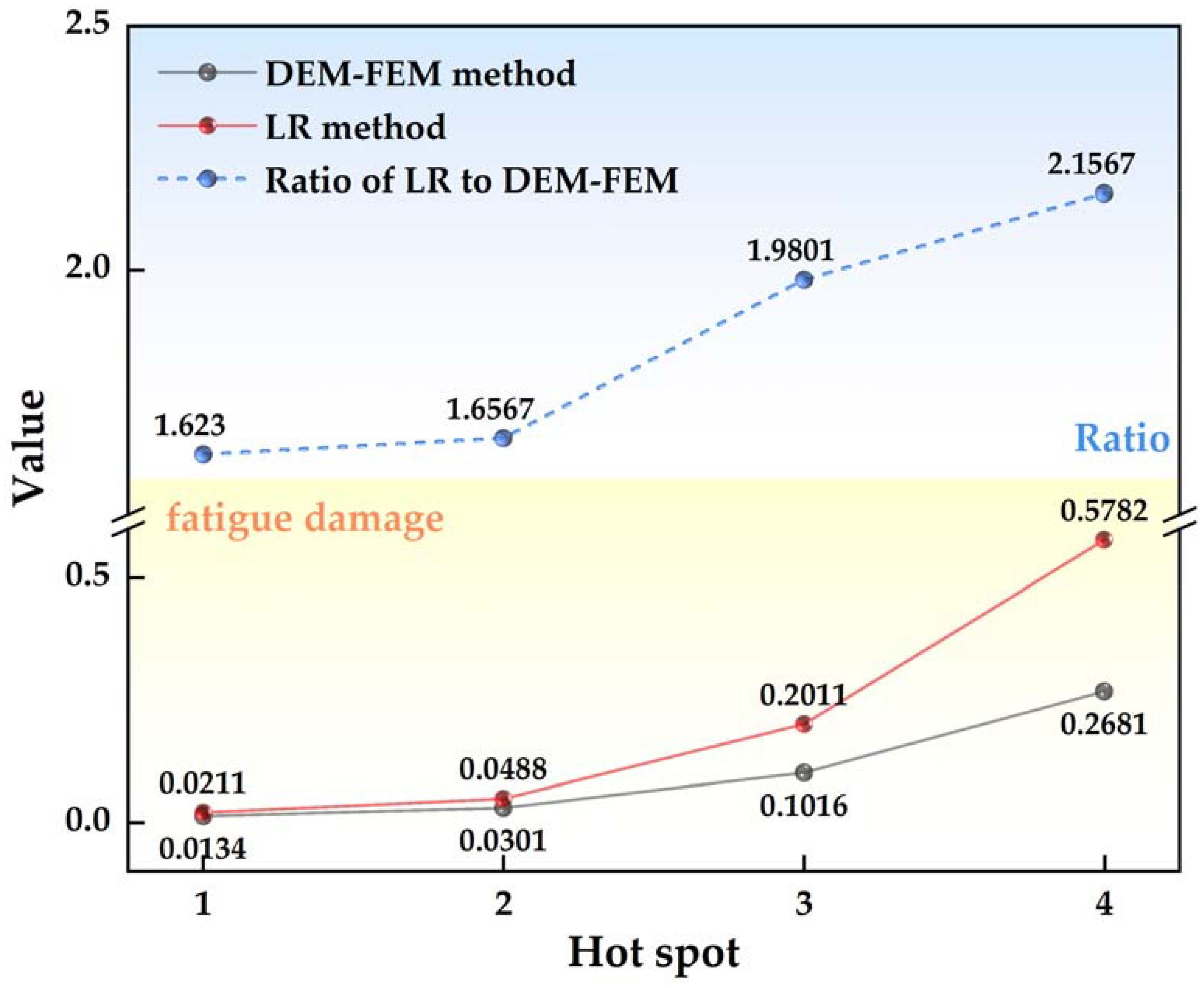
Figure 12. Comparison of fatigue assessment results between the two methods.

7 Conclusions

This paper proposes an ice-induced fatigue damage assessment method for ships navigating in brash ice areas. A brash ice model and a numerical brash ice tank are constructed using the CFD-DEM coupled approach. The validity of the numerical brash ice tank is confirmed by comparing the results with the ice model test conducted by HSVA. Subsequently, focusing on an ice-class cargo ship as the research object, the ice load time histories during ship-ice collisions are calculated. These ice load time histories serve as input for calculating the hot spot stress time histories under different conditions using the FEM. The hot spot stress levels are determined by the rain-flow counting method, and the ice-induced fatigue damage is computed using the S-N curve method based on linear cumulative damage theory. The following conclusions can be drawn from this research:

(1) In the numerical simulation, the accumulation, overturning, and extrusion of brash ice during the ship-ice collision process are observable, consistent with the phenomena observed in the HSVA’s ice tank test. This consistency demonstrates the reliability of the numerical ice tank established using the CFD-DEM approach in this study.

(2) Both the ship speed and sea ice concentration are critical factors influencing ice-induced fatigue stress. As the speed increases, hot spot stress exhibits more peaks within the same time frame, accompanied by an overall stress increase. However, as ship speed continues to rise, the enhanced wave-making effect around the hull moderates the rate of hot spot stress increase. In some instances, a phenomenon of stress reduction may occur at certain hot spots. Sea ice concentration plays a direct role in increasing ship-ice collision frequency, and there is a positive correlation between hot spot stress and sea ice concentration.

(3) Because the bow side directly collides with the brash ice, the hot spots in this area experience the most significant fatigue damage. Moreover, when the bow collides with the brash ice, accumulation and sliding occur near the hull waterline, resulting in relatively high fatigue damage for the hot spot in this vicinity. These areas deserve special attention in structural design.

(4) Comparing the proposed method with the LR method, it becomes evident that the calculation results of the LR method are approximately 1.85 times those of the method proposed in this paper. This is because the LR method makes assumptions and simplifications on ice load prediction and fatigue stress calculation from a safety perspective. While the LR method enhances the speed of ice-induced fatigue assessment, its tendency toward conservatism is noteworthy. It is crucial to emphasize that the comparison with the LR method serves as validation for the rationality of the proposed method rather than a strict accuracy test.

In summary, this study can provide some valuable reference for the fatigue assessment of ships navigating through brash ice channels. However, it is important to note that the research in this paper has certain limitations:

(1) The cohesive and failure models of DEM particles involve numerous microscopic parameters. Further determination of the selection criteria for these parameters and understanding their impact on numerical simulation results is needed.

(2) In the subsequent stages, integrating fatigue assessment with reliability analysis can yield a more practical and engineering-oriented safety evaluation scheme for polar ships.

Data availability statement

The original contributions presented in the study are included in the article/Supplementary Material. Further inquiries can be directed to the corresponding authors.

Author contributions

CZ: Writing – review & editing, Writing – original draft, Methodology, Conceptualization. LC: Writing – original draft, Methodology, Conceptualization. JZ: Writing – review & editing, Methodology, Conceptualization.

Funding

The author(s) declare financial support was received for the research, authorship, and/or publication of this article. This research was funded by the Natural Science Research Program for Universities of Jiangsu Province, China (Grant No. 23KJD580004) and Nantong the Science and Technology Planning Project (Grant No. MS2023088, JZC20183).

Acknowledgments

The authors are particularly grateful to the Mechanics Course Group of Nantong Institute of Technology, the School of Ship and Ocean Engineering, Dalian Maritime University for providing support.

Conflict of interest

The authors declare that the research was conducted in the absence of any commercial or financial relationships that could be construed as a potential conflict of interest.

Publisher’s note

All claims expressed in this article are solely those of the authors and do not necessarily represent those of their affiliated organizations, or those of the publisher, the editors and the reviewers. Any product that may be evaluated in this article, or claim that may be made by its manufacturer, is not guaranteed or endorsed by the publisher.

Supplementary material

The Supplementary Material for this article can be found online at: https://www.frontiersin.org/articles/10.3389/fmars.2024.1416935/full#supplementary-material

Supplementary Table 2 | Hot spot location for ice-induced fatigue assessment.

References

(2011). ShipRight FDA ICE procedures-fatigue induced by ice loading (London, UK: Lloyd's Register).

Google Scholar

(2013). IO 509/12; Brash Ice Tests for a Panmax Bulker with Ice Class 1B (Hamburg, Germany: HSVA).

Google Scholar

(2014). Recommended Procedures and Guidelines: Section 7.5–02-04 for Ice Testing (Copenhagen, Denmark: ITTC).

Google Scholar

Bridges R., Risk K., Zhang S. M. (2006). “Preliminary results of investigation on the fatigue of ship hull structures when navigating in ice,” in the SNAME 7th International Conference and Exhibition on Performance of Ships and Structures in Ice, Banff, Alberta, Canada. doi: 10.5957/ICETECH-2006-142

Crossref Full Text | Google Scholar

Chai W., Leira J. B., Naess A. (2018). Short-term extreme ice loads prediction and fatigue damage evaluation for an icebreaker. Ships Offshore Struct. 13, 127–137. doi: 10.1080/17445302.2018.1427316

Crossref Full Text | Google Scholar

Chang S. (2022). Study on fatigue damage assessment method of ship structure in broken ice fields. Dalian University of Technology, Dalian, China.

Google Scholar

Gang X. H., Tian Y. K., Ji S. P., Guo W., Kou Y. (2021). Experimental analysis on flexural strength of columnar saline model ice. J. Ship Mechan. 16, 143–149. doi: 10.3969/j.issn.1007-7294.2021.03.009

Crossref Full Text | Google Scholar

Gao X. F., Liu X. Y., Xue X. T., Chen N. Z. (2023). Fracture mechanics-based mooring system fatigue analysis for a spar-based floating offshore wind turbine. Ocean Eng. 223, 108618. doi: 10.1016/j.oceaneng.2021.108618

Crossref Full Text | Google Scholar

Guy E., Lasserre F. (2016). Commercial shipping in the Arctic: new perspectives, challenges and regulations. Polar Rec. 52, 294–304. doi: 10.1017/S0032247415001011

Crossref Full Text | Google Scholar

Han Y., Zhu X. Y., Song M. (2023). Fatigue damage calculation of ship hulls caused by ice loads in broken ice fields. Ships Offshore Struct. 19, 1–13. doi: 10.1080/17445302.2022.2164420

Crossref Full Text | Google Scholar

He L., Chai W., Yu X. P., Chen W., Feng S. (2023). Review on random nature of ice loads for Arctic ships. J. Ship Mechan. 27, 1109–1117. doi: 10.3969/j.issn.1007-7294.2023.07.014

Crossref Full Text | Google Scholar

Jeon S., Kim Y. (2022). Fatigue damage estimation of icebreaker ARAON colliding with level ice. Ocean Eng. 257, 111707. doi: 10.1016/j.oceaneng.2022.111707

Crossref Full Text | Google Scholar

Ji S. Y., Wang S. Q. (2023). Rheological behaviors of spherical granular materials based on DEM simulations. Acta Mech. Sin. 39, 722902. doi: 10.1007/s10409-022-22902-x

Crossref Full Text | Google Scholar

Kim J. (2020). Development of the analysis procedure for the ice-induced fatigue damage of a ship in broken ice fields. J. Offshore Mechan. Arctic Eng. 142, 061601. doi: 10.1115/1.4046874

Crossref Full Text | Google Scholar

Kim J., Kim Y. (2019). Numerical simulation on the ice-induced fatigue damage of ship structural members in broken ice fields. Mar. Struct. 66, 83–105. doi: 10.1016/j.marstruc.2019.03.002

Crossref Full Text | Google Scholar

Leira B., Børsheim L., Espeland Ø., Amdahl J. (2009). Ice-load estimation for a ship hull based on continuous response monitoring. Proc. Instit. Mech. Eng. Part M: J. Eng. Maritime Environ. 223, 529–540. doi: 10.1243/14750902JEME141

Crossref Full Text | Google Scholar

Li H., Qian Y., Feng Y. A. (2019). “Numerical method for ice resistance calculation of polar ships navigating in floating ice region,” in International Conference on Offshore Mechanics and Arctic Engineering, USA. doi: 10.1115/OMAE2019-96131

Crossref Full Text | Google Scholar

Li Z. L., Liu Y., Sun S. S., Lu Y. L., Ji S. Y. (2013). Analysis of ship maneuvering performances and ice loads on ship hull with discrete element model in broken-ice fields. Chin. J. Theor. Appl. Mechan. 45, 868–877. doi: 10.6052/0459-1879-13-02

Crossref Full Text | Google Scholar

Liu L., Ji S. Y. (2021). Dilated-polyhedron-based DEM analysis of the ice resistance on ship hulls in escort operations in level ice. Mar. Struct. 80, 103092. doi: 10.1016/j.marstruc.2021.103092

Crossref Full Text | Google Scholar

Liu L., Ji S. Y. (2022). Comparison of sphere-based and dilated-polyhedron-based discrete element methods for the analysis of ship–ice interactions in level ice. Ocean Eng. 224, 110364. doi: 10.1016/j.oceaneng.2021.110364

Crossref Full Text | Google Scholar

Long X., Liu L., Liu S., Ji S. (2021). Discrete element analysis of high-pressure zones of sea ice on vertical structures. J. Mar. Sci. Eng. 9, 348. doi: 10.3390/jmse9030348

Crossref Full Text | Google Scholar

Putra R. U., Basri H., Prakoso A. T., Chandra H., Ammarullah M. I., Akbar I., et al. (2023). Level of activity changes increases the fatigue life of the porous magnesium scaffold, as observed in dynamic immersion tests, over time. Sustainability 15, 823. doi: 10.3390/su15010823

Crossref Full Text | Google Scholar

Suyuthi A., Leira B. J., Riska K. (2013). Fatigue damage of ship hulls due to local ice-induced stresses. Appl. Ocean Res. 42, 87–104. doi: 10.1016/j.apor.2013.05.003

Crossref Full Text | Google Scholar

Tauviqirrahman M., Jamari J., Susilowati S., Pujiastuti C., Setiyana B., Pasaribu A. H., et al. (2022). Performance comparison of newtonian and non-newtonian fluid on a heterogeneous slip/no-slip journal bearing system based on CFD-FSI method. Fluids 7, 225. doi: 10.3390/fluids7070225

Crossref Full Text | Google Scholar

Wang J. W., Chen X. D., He S., Duan Q., Ji S. Y. (2021). An effective method for identifying ice loads on polar ship structures under the influence of failure measuring points. Eng. Mechan. 38, 226–238. doi: 10.6052/j.issn.1000-4750.2020.07.0507

Crossref Full Text | Google Scholar

Wang X., Hu B., Liu L., Ji S. Y. (2023). Discrete element analysis of ice resistances and six-degrees-of-freedom motion response of ships in ice-covered regions. Eng. Mechan. 40, 243–256. doi: 10.6052/j.issn.1000-4750.2021.10.0777

Crossref Full Text | Google Scholar

Wang Y. T., Liu J. J., Hu J. J., Guedes Soares G. C. (2021). Fatigue strength of EH36 steel welded joints and base material at low-temperature. Int. J. Fatigue. 142, 105896. doi: 10.1016/j.ijfatigue.2020.105896

Crossref Full Text | Google Scholar

Yang B. Y. (2022). Research on Prediction Method and Influence Law of Ice Resistance of ship in broken ice conditions. Dalian University of Technology, Dalian, China.

Google Scholar

Yang B. Y., Zhang G. Y., Huang Z. G., Sun Z., Zong Z. (2020). Numerical simulation of the ice resistance in pack ice conditions. Int. J. Comput. Methods 17, 1844005. doi: 10.1142/S021987621844005X

Crossref Full Text | Google Scholar

Zhang J. N., Zhang Y., Shang Y. C., Jin Q., Zhang L. (2022). CFD-DEM based full-scale ship-ice interaction research under FSICR ice condition in restricted brash ice channel. Cold Reg. Sci. Technol. 194, 103454. doi: 10.1016/j.coldregions.2021.103454

Crossref Full Text | Google Scholar

Zhao J. W. (2021). Research on fatigue performance and ice-induced fatigue analysis method of icebreaker structure at low temperatures. Harbin Engineering University, Harbin, China.

Google Scholar

Zhu H., Ji S. Y. (2022). Discrete element simulations of ice load and mooring force on moored structure in level ice. Comput. Model. Eng. Sci. 132, 5–21. doi: 10.32604/cmes.2022.019991

Crossref Full Text | Google Scholar

Zong Z., Yang B. Y., Sun Z., Zhang G. Y. (2020). Experimental study of ship resistance in artificial ice floes. Cold Reg. Sci. Technol. 176, 103102. doi: 10.1016/j.coldregions.2020.103102

Crossref Full Text | Google Scholar