Interannual variability of air-sea CO2 exchange in the Northern Yellow Sea and its underlying mechanisms

A three-dimensional (3-D) physical-biogeochemical-carbon cycle coupled model is used to investigate the interannual variability of the air-sea carbon dioxide (CO₂) flux (FCO₂) in the Northern Yellow Sea (NYS) from 2009 to 2018. The verification of the model indicate that the simulation results for multiple variables exhibit consistency and fit well with the observed data. The study show that although the multi-year average FCO₂ in the NYS is close to the source-sink balance, there are obvious interannual differences between different years. In particular, a relatively strong source of atmospheric CO₂ (1.0 mmol m^–2 d^–1) is exhibited in 2014, while a relatively strong sink of atmospheric CO₂ (–0.7 mmol m^–2 d^–1) emerges in 2016. Mechanism analysis indicates that the abnormally high temperature is the main controlling factor for the relatively high CO₂ efflux rate in the NYS in 2014, while the abnormally low dissolved inorganic carbon (DIC) concentration is the main factor contributing to the relatively high CO₂ influx rate in 2016. Further analysis reveals that the primary reason for the low DIC concentration since the onset of winter in 2016 is the high net decrease rate of DIC in the NYS in 2015, influenced by net community production in the summer and advection processes during the autumn. The abnormally high primary production during the summer of 2015 results in the excessive reduction of DIC concentration through biological processes. In addition, due to the strong northeasterly wind event in November 2015, low-concentration-DIC water from the Yellow Sea (YS) extends into the Bohai Sea (BS). This further leads to higher DIC flux from the NYS into the BS in the upper mixed layer and increases the inflow of low-concentration-DIC water from the Southern Yellow Sea (SYS) into the NYS. These ultimately result in the abnormal reduction of DIC concentration in the upper mixed layer of the NYS during the autumn of 2015. This study enriches our understanding of interannual variability of FCO₂ in the NYS, which will not only help to further reveal the variations of FCO₂ under human activities and climate change, but also provide useful information for guiding the comprehensive assessment of the carbon budget.

1 Introduction

The ocean can absorb approximately 25% of the anthropogenic carbon dioxide (CO₂) emissions (Friedlingstein et al., 2023), playing a crucial role in addressing global warming and achieving carbon neutrality. Although continental shelf seas only account for 10% of the global ocean area, they contribute over 30% of primary production and store 40% of the ocean’s carbon. Continental shelf seas are the regions with the most intense ocean-land-atmosphere interactions (Bauer et al., 2013; Laruelle et al., 2013; Gruber, 2014, 2015, 2018), and they are evidently influenced by human activities. Therefore, quantifying the air-sea CO₂ flux (FCO₂) in continental shelf seas and studying its underlying mechanisms remain key issues in current research. They are crucial for understanding the role of the global carbon cycle in climate change (Bauer et al., 2013; Wang and Zhai, 2021; Dai et al., 2022).

The biogeochemical cycles result in significant spatiotemporal variations in coastal FCO₂. In high-latitude continental shelf seas such as the West Antarctic Peninsula, seasonal and interannual variations are driven by both vertical mixing and primary production. The FCO₂ in this region overall acts as a sink for atmospheric CO₂. During spring and summer, primary production reduces dissolved inorganic carbon (DIC) concentration, making it a net sink for atmospheric CO₂. In contrast, during autumn and winter, physical mixing and net heterotrophy increase DIC concentration in the surface water column, causing it to become a net source of atmospheric CO₂ (Legge et al., 2015, 2017). In the northern Gulf of Mexico and the western Florida shelf, the temporal and spatial variations of the FCO₂ are also primarily influenced by primary production, as well as river discharge, temperature, and coastal water circulation. In this region, it acts as a net sink for atmospheric CO₂ during winter and a source during summer (Hu et al., 2018; Robbins et al., 2018; Kealoha et al., 2020). The North Sea acts as a net CO₂ sink annually. In previous studies, the North Sea is often subdivided into two biogeochemical regimes, a deeper and stratified northern part and a shallower, permanently mixed southern part. The northern region acts as a strong sink for atmospheric CO₂, exporting carbon through the continental shelf pump (Tsunogai et al., 1999) to the deeper Atlantic Ocean (Thomas et al., 2004; Wakelin et al., 2012). In the southern region, the impacts of organic production and decomposition on air-sea CO₂ exchange largely offset each other, resulting in a carbon source-sink balance at an annual scale (Thomas et al., 2004; Schiettecatte et al., 2007; Prowe et al., 2009; Burt et al., 2016). It is evident that the underlying mechanisms of FCO₂ in different continental shelf seas are diverse, thus it needs to be studied according to specific regions. Recent research also emphasizes that understanding the mechanisms of coastal FCO₂ variations is the foremost component in predicting future trends in carbon cycling systems (Keenan et al., 2012; Lauvset et al., 2017).

The Northern Yellow Sea (NYS) is a semi-enclosed and high-productivity continental shelf shallow sea in the northwest Pacific. The NYS serves as a channel for material and energy exchange between the Bohai Sea (BS), adjacent coastal areas, and the open ocean. The NYS is characterized by the East Asian monsoon. Its most prominent hydrological features include the northward-flowing Yellow Sea Warm Current (YSWC) in winter, the NYS Cold Water Mass (NYSCWM), and the significant upwelling along the shelf front (Bao et al., 2009). The thermohaline properties of the NYSCWM are relatively stable. It begins to develop in spring, forms completely in summer, subsides in autumn, and disappears in winter (Ren and Zhan, 2005; Yu et al., 2006).

Numerous research cruises have previously been conducted to investigate the FCO₂ in the NYS. Based on four survey voyages conducted between 2006 and 2007, Xue et al. (2012) concluded that the NYS served as a net source of atmospheric CO₂ throughout the year. On the contrary, based on four surveys conducted by the State Oceanic Administration of China (SOA) in 2009, the Bulletin of Marine Environmental Status of China in 2009 (State Oceanic Administration, 2010) reported that the NYS exhibited a near-balanced annual carbon source-sink state. However, based on four surveys conducted during 2011 – 2012, State Oceanic Administration (2013) showed that the NYS acted as a net annually weak sink for atmospheric CO₂. In light of the 21 fixed-location sampling surveys conducted between 2011 and 2013, the northwestern corner of the NYS (38°40′ N, 122°10′ E) was considered a weak sink of atmospheric CO₂ on an annual scale (Xu et al., 2016). According to 10 mapping cruises conducted between 2011 and 2018, Wang and Zhai (2021) also suggested that the NYS represented one of the weakest marine CO₂ absorbers among various continental shelf CO₂ sinks. There are interannual differences in the understanding of the FCO₂ in the NYS, and whether there is obvious interannual variability in the FCO₂ in the NYS remains to be further studied.

The source-sink pattern of the FCO₂ in the NYS is controlled by multiple factors. Thus, on a seasonal scale, a variety of source-sink patterns still existed. These source-sink transitions occurred not only between different seasons but also within the same season in different survey years (State Oceanic Administration, 2010, 2013; Xue et al., 2012; Xu et al., 2016; Wang and Zhai, 2021). Previous studies indicated that during winter, the FCO₂ in the NYS primarily functioned as a sink for atmospheric CO₂ (State Oceanic Administration, 2013; Xu et al., 2016; Wang and Zhai, 2021), but occasionally behaved as a carbon source (Zhang et al., 2008; Xue et al., 2012; Xu et al., 2016). The source-sink pattern in winter was mainly controlled by the antagonistic effects of low temperature and vertical mixing (Xue et al., 2012; Xu et al., 2016; Wang and Zhai, 2021). In spring, the NYS mainly acted as a carbon sink (State Oceanic Administration, 2010, 2013; Xu et al., 2016; Wang and Zhai, 2021), although a few survey results indicated that it could also be a carbon source (Song et al., 2007; State Oceanic Administration, 2010; Xue et al., 2012). Springtime FCO₂ was mainly influenced by biological processes, nutrient inputs from riverine and atmospheric dry/wet deposition (Zhang, 1994; Shi et al., 2012; Tan and Wang, 2014), high DIC water and sediment input from riverine, and warming processes (Xue et al., 2012; Xu et al., 2016; Wang and Zhai, 2021). In summer, the NYS mainly served as a carbon source (State Oceanic Administration, 2010; Xue and Zhang, 2011; Xue et al., 2012; Xu et al., 2016; Wang and Zhai, 2021), with a minority of surveys indicating it as a carbon sink (State Oceanic Administration, 2013; Xu et al., 2016; Wang and Zhai, 2021). The source-sink pattern in summer was primarily influenced by high temperature, reduced biological processes, and water column stratification (State Oceanic Administration, 2010; Xue and Zhang, 2011, 2013; Xue et al., 2012; Xu et al., 2016; Wang and Zhai, 2021). In autumn, the NYS mainly served as a carbon source (Zhang et al., 2009; State Oceanic Administration, 2010, 2013; Xue et al., 2012; Wang and Zhai, 2021), with only Xu et al. (2016) suggesting it behaved as a carbon sink. The autumn FCO₂ was influenced by increasing vertical mixing and biological processes (Zhang et al., 2009; State Oceanic Administration, 2010, 2013; Xue et al., 2012; Xu et al., 2016; Wang and Zhai, 2021). Consequently, observation data from the cruises indicate that the NYS primarily acts as an atmospheric CO₂ sink during winter and spring, while it serves as a source of atmospheric CO₂ in summer and autumn. This matches Yu et al. (2023) findings on the NYS’s multi-year seasonal carbon dynamics using semi-mechanistic and machine learning methods.

In summary, surface water temperature, biological processes, terrestrial inputs, and hydrodynamic conditions are key factors controlling the source-sink variations of FCO₂ in the NYS (Zhang et al., 2008, 2009; Xu et al., 2016; Wang and Zhai, 2021). Due to these complex physical and biogeochemical processes, the temporal and spatial variations of FCO₂ in the NYS are obvious. As a consequence, different research cruises often lead to conflicting understanding of the source-sink patterns of FCO₂ in the NYS during the same season (Zhang et al., 2008, 2009; State Oceanic Administration, 2010, 2013; Xue and Zhang, 2011; Xue et al., 2012; Xu et al., 2016; Wang and Zhai, 2021; Ko et al., 2022). The contrasting understanding of the source-sink carbon patterns can be attributed to various factors. On the one hand, it’s worth noting that all previously published research on the FCO₂ in the NYS have different sampling times and layouts of stations. This implies that using limited seasonal “snapshot” data to extrapolate the seasonal source-sink status of the NYS may introduce some uncertainties. This highlights the limitation of observation data, but it can be addressed by using well-validated three-dimensional (3-D) regional ocean models. On the other hand, the contradictory understanding of the source-sink patterns of FCO₂ may also stem from the existence of interannual variability in FCO₂ in the NYS. Currently, research on FCO₂ in the NYS mainly focuses on seasonal variations, lacking insights into interannual variability. Therefore, it is particularly important to further enhance our understanding of the interannual variability of FCO₂ in the NYS. Hence, the hindcast simulation from 2009 – 2018 of a 3-D physical-biogeochemical-carbon cycle coupled model will be used to analyze the interannual variability of FCO₂ in NYS. Moreover, The model results will further investigate the influencing factors and underlying mechanisms of anomalous years.

2 Data and methods

2.1 Introduction of the coupled physical-biogeochemical-carbon cycle modeling

We use a 3-D physical-biogeochemical-carbon cycle coupled model in this study. The physical model is based on the Regional Ocean Modeling System (ROMS), which has been widely applied in various research studies (Shchepetkin and McWilliams, 2005; Xiu and Chai, 2010). The simulation domain includes the BS, Yellow Sea (YS), and northern East China Sea (ECS) (Figure 1A), with a horizontal resolution of 2.2 – 4 km and a vertical sigma coordinate with 30 layers and enhanced resolution near the surface and bottom. The initial temperature and salinity are obtained from the World Ocean Atlas 2013 (WOA13) (https://www.nodc.noaa.gov/OC5/woa13/), and the initial velocity and sea level are set to zero. The boundary conditions for temperature, salinity, velocity, and sea level are obtained from the Hybrid Coordinate Ocean Model (HYCOM) (https://www.hycom.org/). Atmospheric forcing (wind stress, shortwave radiation, net heat flux, and freshwater flux) is obtained from the European Centre for Medium-Range Weather Forecasts (ECMWF) (https://www.ecmwf.int/).

Figure 1

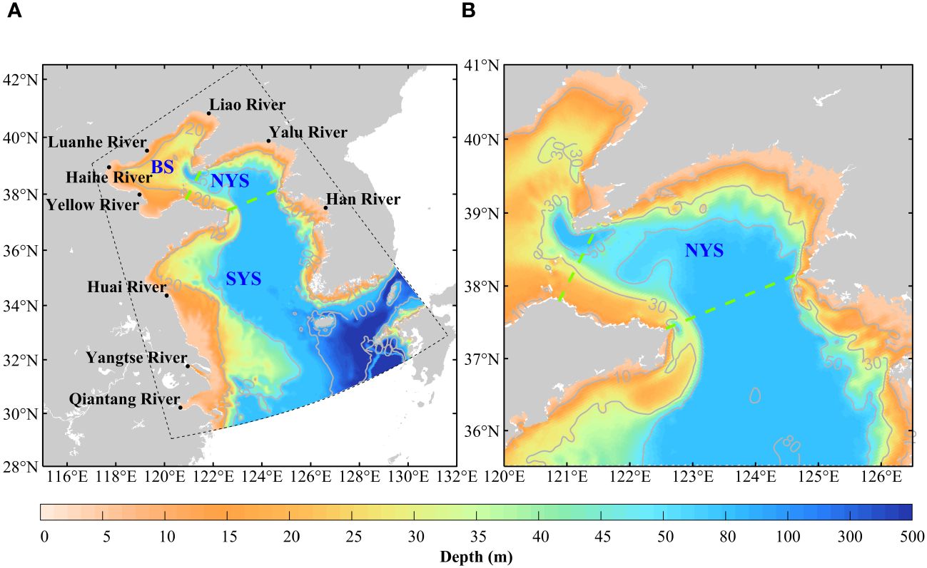
Figure 1 Bathymetric schematics of the model area (A) research area map of the Northern Yellow Sea (NYS) (B). The green dashed lines indicate the boundaries between the NYS and the Bohai Sea (BS), and between the NYS and the Southern Yellow Sea (SYS). The black lack dots in (A) represent the nine rivers included in the model.

The biogeochemical scheme is based on the Carbon, Silicate, and Nitrogen Ecosystem (CoSiNE) model (Chai et al., 2002; Xiu and Chai, 2011), which includes major ecological and carbon chemistry processes. The main ecological forecast variables include four nutrients (silicate, nitrate, phosphate, and ammonium), DIC, total alkalinity (TALK), two phytoplankton groups (diatoms and dinoflagellates), two zooplankton, two detritus types (nitrogen-containing detritus and silicate-containing detritus), and dissolved oxygen (DO). For model configuration, the initial for nitrate, phosphate, and silicate are obtained from the climatological data of WOA13 for January, while DIC and TALK are sourced from the Copernicus Marine Environment Monitoring Service (CMEMS) database (http://marine.copernicus.eu). The values of nitrate, phosphate, silicate, DIC, and TALK at the open boundaries are obtained from the CMEMS database, and atmospheric partial pressure of CO₂ (pCO_2a) data is obtained from the Global Monitoring Laboratory of the National Oceanic and Atmospheric Administration (NOAA).

2.2 Calculation of derived parameters of the carbonate system

In the carbon cycle calculations, DIC and TALK are considered state variables, while the partial pressure of CO₂ in the sea surface (pCO₂) and the FCO₂ are treated as diagnostic variables. The control equation for DIC in the carbon cycle is as follows:

$\begin{array}{ll}\begin{array}{c}\frac{\mathbf{\partial }[DIC]}{\mathbf{\partial }t}=\mathit{\text{adv}}\left(\frac{\mathbf{\partial }[DIC]}{\mathbf{\partial }t}\right)+\mathit{\text{diff}}\left(\frac{\mathbf{\partial }[DIC]}{\mathbf{\partial }t}\right)+\mathit{\text{bio}}\left(\frac{\mathbf{\partial }[DIC]}{\mathbf{\partial }t}\right)\\ +\mathit{\text{atm}}(\frac{\mathbf{\partial }[DIC]}{\mathbf{\partial }t})\end{array}& (1)\end{array}$

where adv and diff are terms due to advection and diffusion, respectively. The bio is a term due to biological processes, and atm represents air-sea CO₂ exchange. The unit of these terms is mmol C m^-3 d^-1. The advection term (adv) primarily describes the transport of substances due to water movement, while the diffusion term (diff) encompasses the diffusion and mixing processes driven by concentration gradients of substances. The advection term is the sum of vertical advection (vadv) and horizontal advection (hadv). The diffusion term can be categorized into vertical mixing (zdf) and lateral mixing (ldf). Since the water selected for the budget analysis in the subsequent text is within the upper mixed layer, the lateral mixing is several orders of magnitude smaller than the vertical mixing, thus lateral mixing can be neglected. The biological processes (bio) refer to net community primary production. In the water column, the biological processes related to DIC include net phytoplankton photosynthesis, zooplankton respiration, and organic matter mineralization. The effect of calcium carbonate formation and dissolution is not included in the biological processes of the current model. There is limited information on the abundance and distribution of planktonic calcifying organisms. Future modeling efforts will consider additional groups of organisms. Therefore, the DIC budget is mainly controlled by four factors: advection (adv), net community production (bio), vertical diffusion (zdf), and air-sea CO₂ exchange (atm).

Before exploring the interannual variability of FCO₂ in the NYS, it is necessary to understand the FCO₂ calculation method in the model, the formula for calculating FCO₂ is as follows:

$\begin{array}{ll}FC{O}_{\mathbf{2}}=\mathit{k}\times \mathit{\alpha }\times (pC{O}_{\mathbf{2}}-pC{O}_{\mathbf{2}a})& (2)\end{array}$

where k represents the CO₂ gas transfer rate at the air-sea interface, it is mainly affected by wind speed (Takahashi et al., 2002; Wanninkhof, 1992; 2014). The α is the solubility of CO₂ gas in seawater, which is mainly affected by temperature (Weiss and Price, 1980). And pCO₂ and pCO_2a represent the partial pressure of CO₂ in surface seawater and the atmosphere, respectively. The sign of their difference determines the direction of CO₂ transfer and also represents the positive or negative of FCO₂. A positive FCO₂ value represents net CO₂ efflux, whereas a negative flux value indicates net CO2 influx. The positive or negative value of FCO₂ is primarily determined by the pCO₂. This is because the spatiotemporal variability of partial pressure of CO₂ in the atmosphere is relatively small compared to that in the surface seawater (Tsunogai et al., 1997).

According to the CO2SYS program proposed by Lewis and Wallace (1998), the pCO₂ can be calculated using temperature, salinity, DIC, and TALK. Among these parameters, salinity and TALK are relatively conservative. In the subsequent exploration of the impact of controlling temperature on pCO₂. In the calculations, the salinity, DIC, and TALK values are based on the regional averages for the NYS from 2009 to 2018. The specific values are as follows: salinity is 32 Practical Salinity Units (PSU), DIC is 2111 µmol kg^–1, and TALK is 2304 µmol kg^–1.

In addition to the methods mentioned above, the factors affecting the variation in pCO₂ can be divided into thermal and non-thermal effects (Takahashi et al., 1993, 2002). Among them, the thermal effect refers to the thermodynamic regulation of temperature on the pCO₂. As the temperature rises, the pCO₂ increases slightly. Takahashi et al. (1993, 2002) proposed that the sensitivity of pCO₂ to temperature follows the relationship:

$\begin{array}{ll}\frac{\mathbf{\partial }\mathbf{\text{ ln }}(pC{O}_{\mathbf{2}})}{\mathbf{\partial }T}=\mathbf{0.0423}{\mathit{\text{ °C}}}^{-\mathbf{1}}& (3)\end{array}$

We deform Equation 3 to obtain Equation 4 as below. This implies the amount of pCO₂ change caused by temperature is:

$\begin{array}{ll}\Delta pC{O}_{\mathbf{2},T}=({\mathit{\text{e}}}^{\mathbf{0.0423}\mathit{\Delta }\mathit{\text{T}}}-\mathbf{1})pC{O}_{\mathbf{2}}& (4)\end{array}$

2.3 Model validation

The model used in this study runs from 2006 to 2018, After the model is stable, data for the ten years from 2009 to 2018, are selected to analyze the interannual variations of FCO₂ in the NYS. The tidal, flow field, temperature-salinity, chlorophyll-a, pH, and nutrient simulations of the ROMS-CoSiNE model have been thoroughly evaluated in previous studies (Luo et al., 2019; Zhang et al., 2020; Li et al., 2021; Guo et al., 2022; Zhang et al., 2022). These evaluations indicate that the ROMS-CoSiNE model effectively reproduces the spatiotemporal distribution characteristics of physical and ecological environmental factors in the Bohai and Yellow Seas. Moreover, this coupled model has been extensively utilized in studies of the physical ecological systems in the Bohai and Yellow Seas (Zhang et al., 2020; Li et al., 2021; Guo et al., 2022; Zhang et al., 2022).

In this paper, the model validation area includes the NYS and its adjacent seas, since the DIC advection flux is influenced by the DIC concentration in the northern and southern parts of the NYS. The data used for model validation in this paper are detailed in Table 1. We first use the data to evaluate the spatial distribution and seasonal variations of simulated DIC and pCO₂ (Figures 2, 3). Additionally, we use these data to analyze the variations of DIC and pCO₂ in the NYS over the past few years (Figures 4A, B).

Table 1

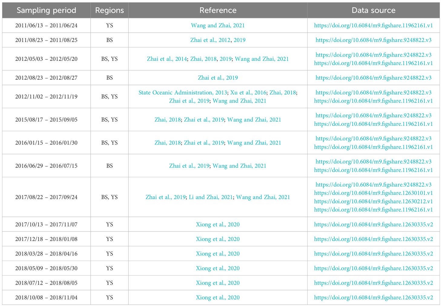
Table 1 Observation data of dissolved inorganic carbon (DIC) and partial pressure of CO₂ in the sea surface (pCO₂) of the Bohai Sea (BS) and the Yellow Sea (YS) from 2011 to 2018.

Figure 2

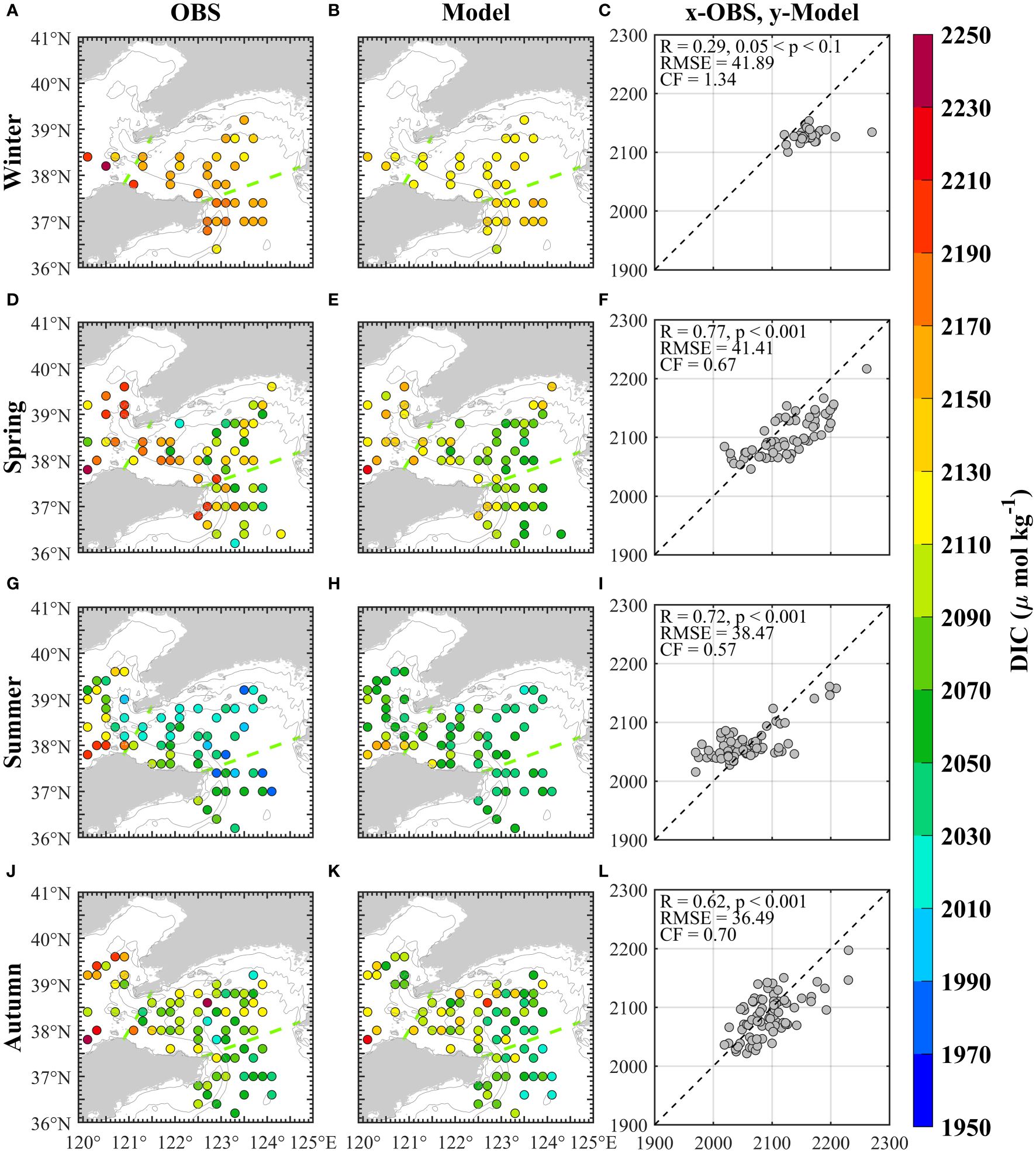
Figure 2 The comparison between observation and simulation of the sea surface dissolved inorganic carbon (DIC) concentration in the Northern Yellow Sea (NYS) and its adjacent seas; (A–C) winter, (D–F) spring, (G–I) summer, (J–L) autumn. The first column is the observed data. The second column is the simulated data corresponding to the observed spatiotemporal points. The third column is the scatter plot of the observed and simulated data, with the x-axis for observations and the y-axis for simulations. The green dashed lines in the first and second columns of the figures represent the NYS boundary. R represents the Pearson correlation coefficient; p represents the confidence in statistical significance tests; RMSE represents the Root Mean Square Error; CF represents the Cost Function.

Figure 3

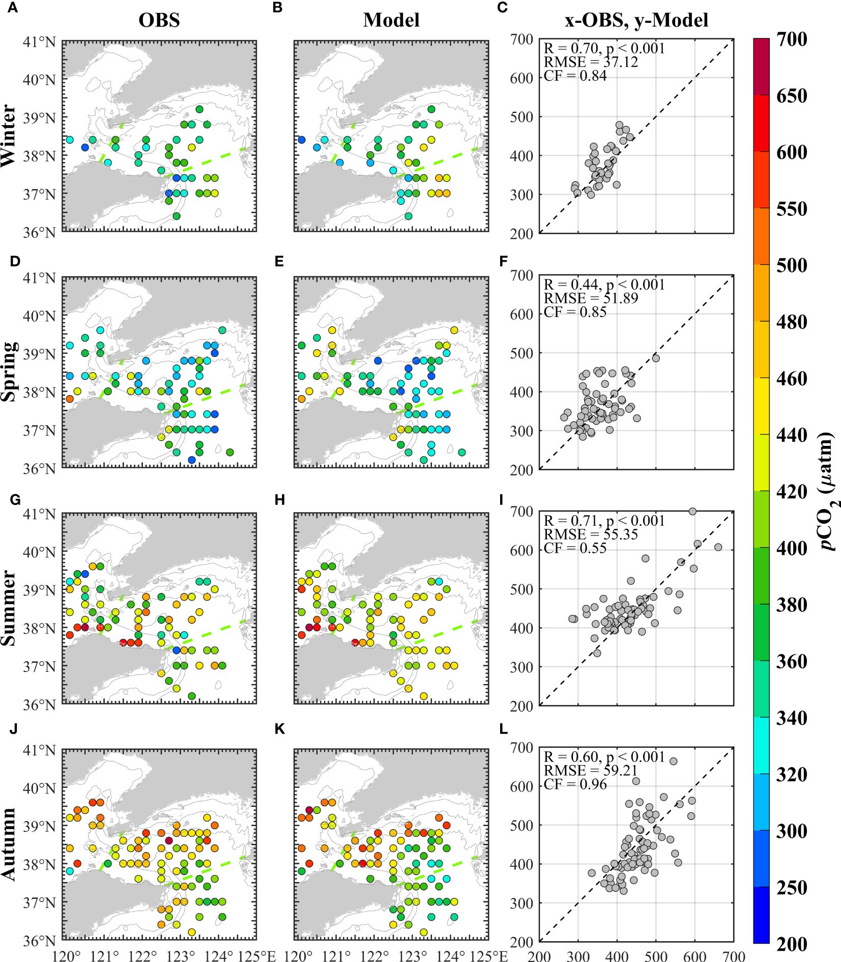
Figure 3 The comparison between observation and simulation of the sea surface partial pressure of CO₂ (pCO₂) in the Northern Yellow Sea (NYS) and its adjacent seas; (A–C) winter, (D–F) spring, (G–I) summer, (J–L) autumn. The first column is the observed data. The second column is the simulated data corresponding to the observed spatiotemporal points. The third column is the scatter plot of the observed and simulated data, with the x-axis for observations and the y-axis for simulations. The green dashed lines in the first and second columns of the figures represent the NYS boundary.

Figure 4

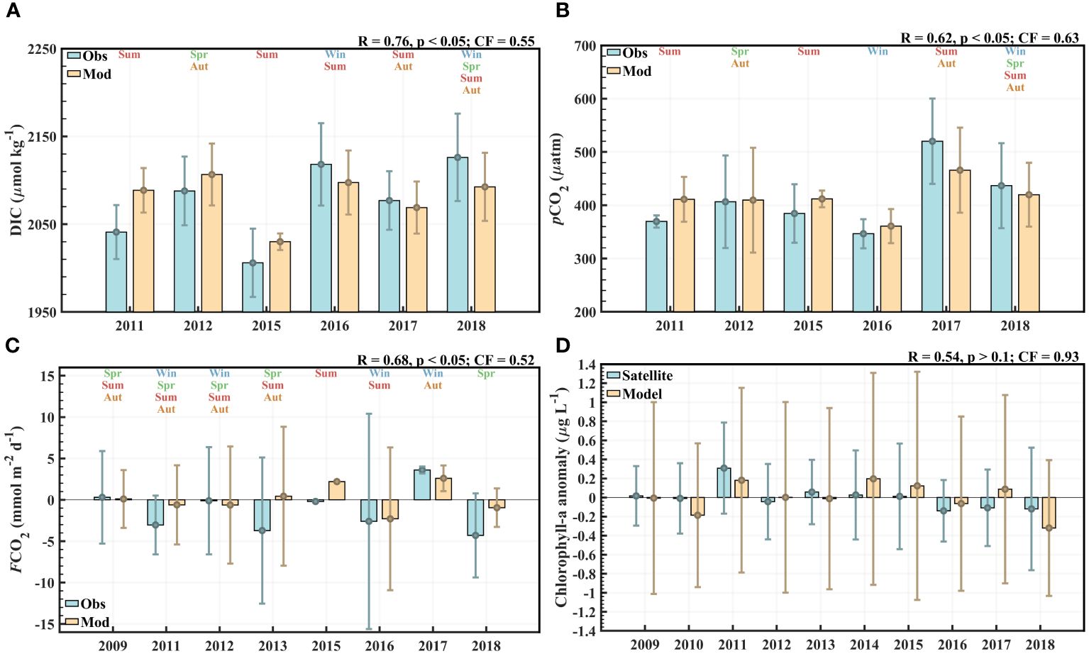
Figure 4 The annual mean and standard deviation of observed and model values in the in the Northern Yellow Sea (NYS), (A) dissolved inorganic carbon (DIC), (B) partial pressure of CO₂ in the sea surface (pCO₂), (C) air-sea CO₂ flux (FCO₂), (D) chlorophyll-a anomalies. The colored texts in (A–C) represent the seasonal information of the data contained in each year.

In order to further evaluate the reliability of the model, we analyze the multi-year variations of FCO₂ in the NYS based on the historical data (State Oceanic Administration, 2010; Xu et al., 2016; Wang and Zhai, 2021) collected from 2009 to 2018 (Figure 4C). Additionally, we evaluate the model’s chlorophyll-a by using satellite remote sensing data from the Ocean Colour Climate Change Initiative (OC-CCI, http://www.esa-oceancolour-cci.org) project covering 2009 – 2018 (Figure 4D). Through assessing simulated DIC, pCO₂, FCO₂, and chlorophyll-a, we optimize model parameters to enhance the simulation accuracy of the ROMS-CoSiNE model for the carbon cycle in the NYS. These provide reliable data support for a better understanding of the dynamic changes in the marine carbon cycle.

2.3.1 Data and processing methods

The data used for the model’s DIC concentration and pCO₂ validation in this study consists of observation data from 15 cruises in the Bohai and Yellow Seas from 2011 to 2018 (Table 1). The sampling period, distribution region, literature and data sources for the cruise data are shown in detail in Table 1. Table 1 includes 2 winter cruises, 3 spring cruises, 6 summer cruises, and 4 autumn cruises, with 8 cruises in the BS, 12 cruises in the NYS, and 12 cruises in the South Yellow Sea (SYS).

During the processing of sampling station data from 15 cruise surveys for DIC concentration and pCO₂, the observed and model data are processed as follows: first, the model results corresponding to the sampling dates of the observation data are selected for comparison. Then, the model results are interpolated to match the spatial coordinates of latitude, longitude, and water depth corresponding to the sampling locations of the observation data. This ensures temporal and spatial consistency between the observed and model data. After obtaining point-to-point matched data between the model and observations, the observation data belonging to the same season are merged into one table, divided into four parts: winter, spring, summer, and autumn. The model data are processed in the same way. Next, both the observed and model data are separately gridded onto a 0.2-degree grid. The gridding principle is that each data sample can only belong to one grid. If a grid contains more than three samples, the three times standard deviation principle is applied to identify and eliminate outliers. Finally, the value of each grid is the average value of the valid sample data within that grid. This data processing workflow provides reliable data foundations for model validation and comparative analysis.

During the validation of the model FCO₂ in the NYS, the data processing procedure is as follows. From 2009 to 2018, there were only 35 observed FCO₂ data in the NYS: 4 from State Oceanic Administration (2010), 10 from Wang and Zhai (2021), and 21 from Xu et al. (2016). Among them, the FCO₂ data from State Oceanic Administration (2010) and Wang and Zhai (2021) represent the monthly average data of the NYS in a specific year. Therefore, the model’s average FCO₂ results in the NYS for the corresponding years and months are used for comparison. The data from Xu et al. (2016) are collected at the A4HDYD station (38°40′ N, 122°10′ E) in the NYS, so the model grid data closest to this station are selected for comparison.

In Luo et al. (2019), the spatial distribution and seasonal variation of chlorophyll-a in the model have already been validated. To further validate the interannual variation of chlorophyll-a from 2009 to 2018, this study uses satellite remote sensing chlorophyll-a data from the Ocean Colour Climate Change Initiative (OC-CCI, https://www.oceancolour.org/). Firstly, the satellite data is interpolated to the model grid. As the missing satellite data in different years is inconsistent, it is necessary to mark the missing data regions in the satellite data from 2009 to 2018, similar treatment is performed on the simulated values to ensure that the coverage area of the model data and the satellite data are completely the same for comparison. Finally, the annual average values of chlorophyll-a for both satellite and model data are obtained. The standard deviation for each year is calculated using the results of all 12 months within that year. The anomaly of satellite chlorophyll-a is calculated as the chlorophyll-a value of a specific year minus the multi-year average chlorophyll-a value of the satellite. Similarly, the anomaly value of simulated chlorophyll-a is calculated as the model’s chlorophyll-a value of a specific year minus the model’s multi-year average chlorophyll-a value. Finally, the interannual variability of chlorophyll-a anomalies is compared. Comparing anomalies can better reflect interannual differences. This comparative approach can better evaluate the model’s ability to simulate interannual variations in chlorophyll-a.

The cost function (CF) is used as an objective indicator to evaluate model performance in model validation. CF is the sum of the absolute values of the differences between observations and models, divided by the product of the number and the standard deviation of observations. The formula is as follows:

$\begin{array}{ll}\mathit{C}\mathit{F}=\frac{{\sum }_{i=1}^N\mid Mo{d}_i-Ob{s}_i\mid }{N{\sigma }_{Obs}}& (5)\end{array}$

Mod_i represents the model results, Obs_i represents the observed results, N is the number of observations, and σ_obs represents the standard deviation of the observed data (Equation 5). CF quantifies the goodness of fit between the observed and model results, with the following standard ranges: 0 – 1 (excellent/very good), 1 – 2 (good), 2 – 3 (reasonable), > 3 (poor/not good) (Radach and Moll, 2006).

2.3.2 Validation of dissolved inorganic carbon

Overall, the ROMS-CoSiNE model shows good consistency with the simulated and observed results of DIC concentration (Figure 2) in the NYS and its adjacent seas. From Figure 2, it can be observed that the Pearson correlation coefficients between the model and observations are mainly in the in the range of 0.62 – 0.77 (p< 0.001), indicating a strong correlation. Meanwhile, the root mean square errors (RMSE) for all four seasons range from 36 to 42 µmol kg^–1. The CF values for spring, summer, and autumn are within the range of 0.57 to 0.70. These results suggest that the model has relatively small deviations between the model results and the observed values. Considering the results of the above model evaluation indicators, it further validates the relatively good performance of the ROMS-CoSiNE model in simulating DIC concentration in the NYS and its adjacent seas. The model can capture the seasonal and spatial variations of the observed data relatively accurately. In terms of spatial distribution, DIC concentration displays a pattern of higher levels in the north and lower levels in the south, with the BS having a higher DIC concentration compared to the NYS and the northern part of the SYS. In the NYS and its adjacent seas, DIC concentration exhibits a nearshore-high and offshore-low distribution pattern. The results of Wang and Zhai (2021) also indicated that DIC concentration gradually increased from south to north, indicating a consistent spatial distribution of DIC concentration between the model and observations. Overall, the distribution of DIC in the NYS and its adjacent seas ranges from 2000 to 2200 µmol kg^–1. In the NYS, the ranges of the simulation DIC concentrations for each season closely match those observed. Seasonally, DIC concentration is relatively higher in winter and spring, and lower in summer and autumn, with the lowest DIC concentration occurring in summer, which is consistent with the seasonal variation of DIC described in Wang and Zhai (2021). During dry seasons (winter and spring) DIC concentration tend to be higher, while during wet seasons (summer and autumn) have lower DIC concentration. The correlation coefficient for DIC in winter is relatively low, and the CF is slightly greater than 1. This may be due to the limited number of observation samples for winter DIC validation, which affects the reliability of the validation results.

To further evaluate the simulation performance in different years, Figure 4A compares the annual mean values and standard deviations of the observed and simulated DIC concentration in the NYS. Notably, the spatiotemporal information of the observed and simulated data is well matched by statistical analysis. The seasonal information of the data contained in each year is also shown in Figure 4A. The data for 2011 and 2015 only includes summer, 2012 includes spring and autumn, 2016 comprises winter and summer, 2017 encompasses summer and autumn, and 2018 covers all four seasons. The R and CF values marked in the upper right corner of Figure 4A are calculated using all the corresponding station data in the NYS from observations and model simulations across these years. The Pearson correlation coefficient is 0.76 (p< 0.001) and the CF value is 0.55 (Figure 4A). This indicates that the model performs well in simulating DIC concentration. Figure 4A further demonstrates that the observed and simulated annual mean DIC concentrations in the NYS are similar, and the interannual variation trends are consistent. Notably, the DIC concentration in the summer of 2015 is lower than in the summer of 2011. However, due to differences in seasonal coverage of observation data across different years, direct comparison of annual mean values can not accurately reflect the real interannual variations. Nevertheless, this comparison is still very important. By comprehensively considering multi-year data, the model can still reveal the general trend of interannual variations in DIC concentration, even with incomplete seasonal information. This phenomenon not only aids in our deeper understanding of the interannual variations in the carbon cycle of the NYS, but also further demonstrates the robust simulation capability of the ROMS-CoSiNE model for DIC concentration.

2.3.3 Validation of the sea surface partial pressure of CO₂

The verification results of surface pCO₂ are shown in Figure 3. From Figure 3, it can be observed that all correlation coefficients between the model and observations are between 0.44 and 0.71 (p< 0.001). Moreover, the RMSE for all four seasons ranges from 37 to 59 µatm. The CF values for all four seasons are all less than 1. These results indicate a high level of fit between the model and the seasonal variations of pCO₂. In terms of spatial distribution, the simulated results of pCO₂ show a high similarity to the observed data, showing a pattern of higher values near the coast and lower values in offshore areas. Overall, the simulated and observed pCO₂ values in the NYS and its adjacent seas are generally distributed in the range of 300 to 500 µatm. In the NYS, the ranges of the simulation pCO₂ are relatively consistent with the observations across all seasons. Specifically, pCO₂ is relatively higher in summer and autumn, while it is relatively lower in winter and spring, following the pattern of summer > autumn > spring > winter in terms of pCO₂ variations. A further assessment of the model’s performance in simulating the pCO₂ of the NYS for different years is conducted (Figure 4B). The spatiotemporal information for both the model and observation data is well matched for statistical analysis. Due to difficulties in obtaining observation data, the data for 2011 and 2015 only includes summer, 2016 only includes winter, 2012 comprises spring and autumn, 2017 includes summer and autumn, and 2018 covers all four seasons. The R and CF values marked in the upper right corner of Figure 4B are also calculated using all the corresponding station data in the NYS from observations and model simulations across these years. The Pearson correlation coefficient is 0.62 (p< 0.001) and the CF value is 0.63 (Figure 4B). This indicates that the model performs well in simulating pCO₂. By comprehensively considering multi-year data, even with incomplete seasonal information, the observed and simulated annual mean pCO₂ in the NYS are similar, and the model can capture the interannual variability observed. Despite certain limitations, this comparison enhances the reliability of the model in simulating pCO₂.

2.3.4 Validation of air-sea CO₂ flux and chlorophyll-a

The seasonal information of the data contained in each year is already shown in Figure 4C. The R and CF values marked in the upper right corner of Figure 4C are calculated from the 35 observed values and the 35 corresponding simulated values of FCO₂ over these years. From Figure 4C, it can be observed that the correlation coefficient is 0.68 (p< 0.001) and the CF value is 0.63 (Figure 4C). And if we only use the 14 average regional data from the NYS provided by State Oceanic Administration (2010) and Wang and Zhai (2021), the correlation coefficient will be 0.92 (p< 0.001) and the CF value will be 0.43. From Figure 4C, it can be seen that the annual mean FCO₂ values from observation and model are relatively close, and the range of annual FCO₂ standard deviations is also similar. The source-sink patterns of the NYS in the model are generally consistent with the observations. However, in 2013, the observed value in the NYS indicates a sink, while the model value indicates a source. The FCO₂ data for 2013 come from Xu et al. (2016) and include six values for March, May, July, September, November, and December. Only the source-sink patterns in July and November of 2013 are opposite between the observations and the model. In summer (July), the FCO₂ result from Xu et al. (2016) is –0.5 mmol m^–2 d^–1, while the model result is 0.8 mmol m^–2 d^–1. In autumn (November), the FCO₂ result from Xu et al. (2016) is –8.1 mmol m^–2 d^–1, while the model result is 12.5 mmol m^–2 d^–1. However, most of the previous studies indicate that the NYS behaves as a source during summer and autumn (Zhang et al., 2009; State Oceanic Administration, 2010; Xue et al., 2012; Wang and Zhai, 2021; Yu et al., 2023). These comparison results indicate that the model performs well in simulating FCO₂.

In addition, we also assess the interannual variations of chlorophyll-a anomalies using the OC-CCI satellite remote sensing data and model data (Figure 4D). The annual variations of chlorophyll-a anomalies in OC-CCI data and model data are generally consistent, with a CF value of 0.93 between them (Figure 4D). Since this value is less than 1, it indicates that the error between the model’s simulated values and the OC-CCI data is relatively small. Therefore, it can be concluded that the model is able to adequately fit the annual variation characteristics of chlorophyll-a anomalies.

In conclusion, the model exhibits high consistency and fits with observation data in terms of seasonal variations and spatial distribution of DIC and pCO₂. Furthermore, the model also can capture the interannual variation characteristics of DIC, pCO₂, FCO₂, and chlorophyll-a anomalies. These indicate that the model can be effectively applied to further analyze the interannual variability of FCO₂ in the NYS, as well as mechanism analysis.

3 Results

3.1 Interannual variations of air-sea CO₂ flux in the Northern Yellow Sea

The results of FCO₂ in the NYS from 2009 to 2018 are shown in Figure 5. The multi-year average results for each season show a clear carbon source/sink transformation with seasonal variations. The FCO₂ values for winter, spring, summer, and autumn are –2.4 mmol m^–2 d^–1, –3.4 mmol m^–2 d^–1, 2.5mmol m^–2 d^–1, and 3.7 mmol m^–2 d^–1, respectively (Figure 5A). These results fall within the range of FCO₂ variations reported in previous studies. It is worth noting that the NYS acts as a carbon sink during winter and spring, which is consistent with previous research (State Oceanic Administration, 2013; Xu et al., 2016; Wang and Zhai, 2021; Yu et al., 2023). On the other hand, it acts as a carbon source during summer and autumn, which aligns with previous studies (State Oceanic Administration, 2010; Xue and Zhang, 2011; Xue et al., 2012; Wang and Zhai, 2021; Yu et al., 2023). Overall, the carbon source-sink patterns in the four seasons of the NYS are consistent with previous research.

Figure 5

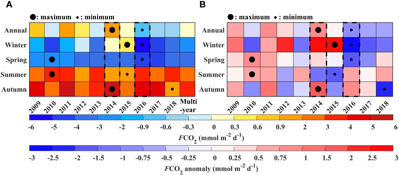
Figure 5 Interannual variations of air-sea CO₂ flux (FCO₂) in the Northern Yellow Sea (NYS) from 2009 to 2018; (A) each color block’s value represents the grid area-weighted average of FCO₂ for the NYS region, (B) each color block’s value represents the grid area-weighted average of FCO₂ anomalies for the NYS region. FCO₂ anomalies are the difference between the FCO₂ in a given season or year and its multi-year average. The first row in (A, B) represents annual averages, and the second, third, fourth, and fifth rows represent results for winter, spring, summer, and autumn, respectively. For winter, the results are based on the average of December of the previous year and January and February of the current year. Each column represents a year, and the last column represents the multi-year average results from 2009 to 2018. Large black solid dots represent the multi-year maximum values, while small black solid dots represent the multi-year minimum values.

Overall, the multi-year average results indicate that the FCO₂ in the NYS is 0.1 mmol m^–2 d^–1 (Figure 5A), suggesting a close-to-balanced carbon source-sink equilibrium and a very weak carbon source. During the simulated period from 2009 to 2018, the FCO₂ in the NYS exhibits obvious interannual variations and multiple transitions in source and sink patterns. Specifically, in 2014, the NYS exhibited a relatively strong source of atmospheric CO₂, with an annual average carbon source intensity of 1.0 mmol m^–2 d^–1 (Figure 5A), which is 0.9 mmol m^–2 d^–1 (Figure 5B) higher than the multi-year average FCO₂. In contrast, 2016 is characterized by a relatively strong sink of atmospheric CO₂, with a carbon sink intensity of –0.7 mmol m^–2 d^–1 (Figure 5A), which is 0.8 mmol m^–2 d^–1 (Figure 5B) lower than the multi-year average FCO₂.

Further analysis of the interannual variations in each season reveals that, except for weak source signals in the winter of 2014 and 2015, the NYS acts as a sink for the rest of the years. The winter of 2016 stands out as an anomalously strong sink (–5.6 mmol m^–2 d^–1), which is 3.2 mmol m^–2 d^–1 weaker than the multi-year winter average (Figure 5A). In contrast, the interannual variations in spring indicate that the NYS has consistently acted as a sink for atmospheric CO₂ throughout the decade, with the spring of 2016 being an abnormally strong sink at –4.9 mmol m^–2 d^–1 (Figure 5A). And this value is 1.5 mmol m^–2 d^–1 lower than the multi-year spring average (Figure 5B). In addition, the interannual variations in summer indicate that the NYS acts as a source of atmospheric CO₂ over the past decade. However, the carbon source intensity in the summer of 2015 is obviously weaker than the multi-year summer average, with a reduction of 1.5 mmol m^–2 d^–1 (Figures 5A, B). Moreover, the interannual variations in autumn also show the NYS as a source of atmospheric CO₂, with the autumn of 2014 being an abnormally strong source at 5.4 mmol m^–2 d^–1 (Figure 5A).

The interannual variations reveal complex changes in FCO₂ in the NYS, especially in anomalous years of carbon source-sink transitions. Further research is needed to help understand the controlling factors and driving mechanisms.

3.2 Interannual variations of the sea surface partial pressure of CO₂ in the Northern Yellow Sea

The results of pCO₂ in the NYS from 2009 to 2018 are shown in Figure 6. The seasonal variations of the pCO₂ in the NYS are very obvious. The pCO₂ values for winter, spring, summer, and autumn are 386 µatm, 381 µatm, 446 µatm, and 441 µatm, respectively (Figure 6A). With other conditions remaining unchanged, lower pCO₂ usually results in a lower FCO₂ values, while higher pCO₂ generally leads to a higher FCO₂ values. This is also consistent with the conclusion in Figure 5A that the FCO₂ in the NYS acts as a sink in winter and spring, and as a source in summer and autumn.

Figure 6

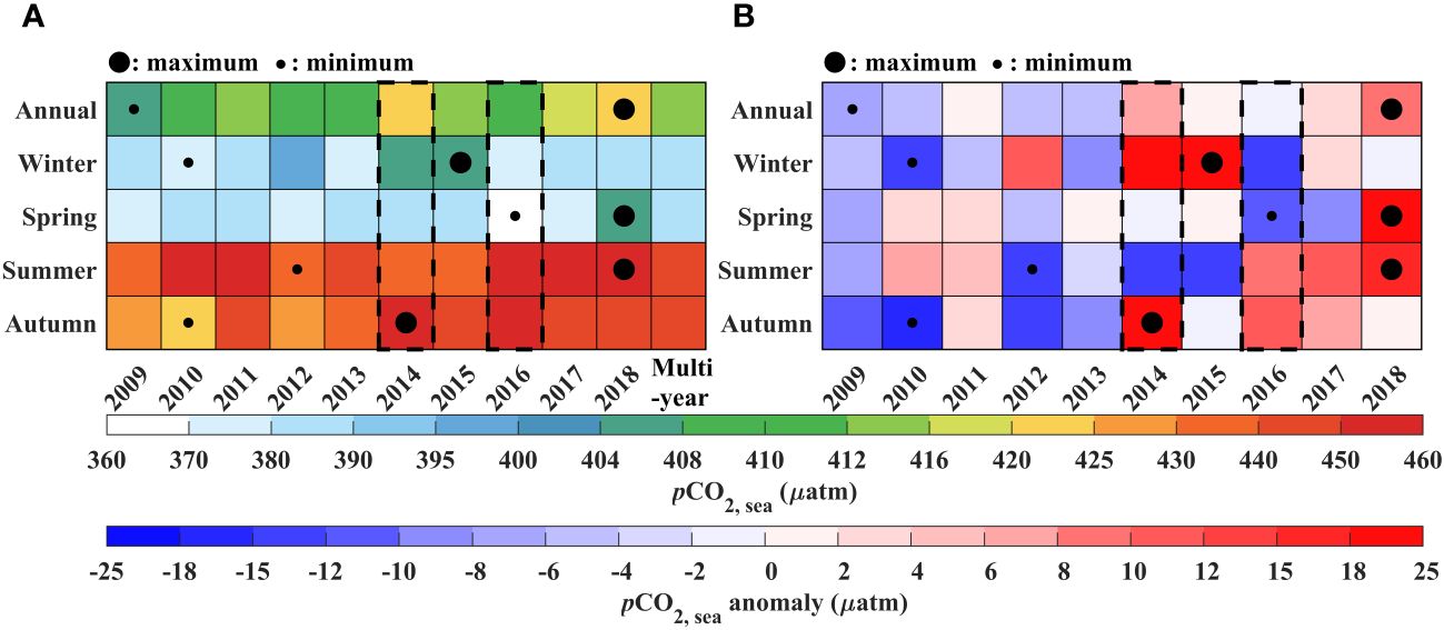
Figure 6 Interannual variations of sea surface partial pressure of CO₂ (pCO₂) in the Northern Yellow Sea (NYS) from 2009 to 2018; (A) each color block’s value represents the grid area-weighted average of FCO₂ for the NYS region, (B) each color block’s value represents the grid area-weighted average of FCO₂ anomalies for the NYS region. The pCO₂ anomalies are the difference between the pCO₂ in a given season or year and its multi-year average. The first row in (A, B) represents annual averages, and the second, third, fourth, and fifth rows represent results for winter, spring, summer, and autumn, respectively. For winter, the results are based on the average of December of the previous year and January and February of the current year. Each column represents a year, and the last column represents the multi-year average results from 2009 to 2018. Large black solid dots represent the multi-year maximum values, while small black solid dots represent the multi-year minimum values.

On the multi-year average results, the pCO₂ in the NYS exhibits an interannual variation. Specifically, from 2009 to 2018, the highest pCO₂ is 423 µatm, and in 2014, the pCO₂ of the NYS is the second highest at 421 µatm (Figure 6A). Moreover, as shown in Figure 5, 2014 is also a year with relatively high FCO₂ (Figure 5). Additionally, the pCO₂ in 2016 is lower than the multi-year average results (Figure 6A), and the FCO₂ in 2016 is also relatively lower than the multi-year average (Figure 5). Further analysis of the interannual variations in each season reveals that, in the autumn of 2014, the pCO₂ reaches the highest value among multi-year autumns, 25 µatm higher than the multi-year autumn average (Figure 6B). Furthermore, the FCO₂ in the autumn of 2014 is also the highest among all autumn seasons (Figure 5). Moreover, in the winter and spring of 2016, pCO₂ was abnormally low (Figure 6), and the NYS also act as an abnormally strong carbon sink during the same period (Figure 5). In the summer of 2015, pCO₂ is 12 µatm lower than the multi-year summer average (Figure 6B). This is also consistent with the obviously reduction of carbon source intensity in the summer of 2015 (Figure 5).

4 Discussion

4.1 Analysis of the influencing factors of the carbon source-sink interannual variation

The FCO₂ is a parameter reflecting the CO₂ exchange between the ocean and the atmosphere. It is calculated as the product of the gas transmission rate, the solubility of CO₂ in seawater, and the partial pressure difference of CO₂ between the ocean and the atmosphere (Equation 2). Since the first two parameters are strictly positive, they only affect the intensity of FCO₂ and do not cause the change of in the source-sink pattern (Gray et al., 2018; Gruber et al., 2019). However, from 2014 to 2016, there was a shift in the source-sink pattern of FCO₂, indicating that the third parameter, the CO₂ partial pressure gradient at the ocean-atmosphere interface, is the key factor driving the change of the source-sink pattern during this period. Compared with the temporal and spatial variability of pCO₂, the spatiotemporal variability of pCO_2a is relatively small (Tsunogai et al., 1997). Therefore, the main factor causing the source-sink transition of FCO₂ from 2014 to 2016 is the pCO₂. The variation of pCO₂ can be attributed to the effects of thermal and non-thermal factors. The thermal effect refers to the thermodynamic adjustment of pCO₂ by sea temperature, where pCO₂ increases slightly with the increase of temperature. The non-thermal effect is mainly influenced by parameters of the carbonate system, such as DIC and TALK, with TALK being relatively conservative and exhibiting small temporal and spatial variations, hence pCO₂ is primarily influenced by DIC. Jiang et al. (2013) also indicate that the net changes in pCO₂ depend on the balance between SST and DIC variations, which may offset each other. Additionally, Omar et al. (2019) found that DIC is the main driving factor for the interannual variability of pCO₂ in the North Sea, while temperature has a secondary effect.

Figure 7 analyzes the interannual variations of the two main factors influencing FCO₂: temperature anomalies and DIC anomalies. The interannual variability in temperature anomalies shows that the year with the highest temperature is 2014 (Figure 7A). The average temperature in 2014 is 0.5° higher than the multi-year average (13.1°C). Particularly in spring and summer, the temperature in 2014 reaches the highest value in 2009 – 2018, exceeding the multi-year average by 0.8°C and 0.3°C, respectively. Additionally, the temperature in winter and autumn are obviously higher than the multi-year average temperature of each season, rising by 0.8° and 0.3°C, respectively. Since 2014 is a year of abnormally high temperatures in the NYS, and it is also the year of relatively high FCO₂ (Figure 5), it is preliminarily speculated that the relatively high FCO₂ in 2014 is caused by the abnormally high temperatures. The following sections will quantitatively analyze the impact of temperature increase using the empirical formulas proposed by Takahashi et al. (1993, 2002) and the CO2SYS program proposed by Lewis and Wallace (1998). Furthermore, 2016 is the year with the highest winter temperatures among all winters, with temperatures exceeding the long-term average by 0.8°C. Similarly, 2015 has the highest autumn temperatures among all autumns, with a temperature increase of 0.5° compared to the multi-year average for autumn.

Figure 7

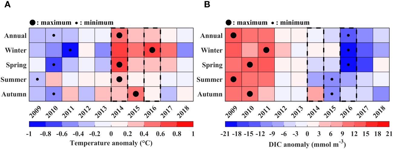
Figure 7 Anomalies of influencing factors of air-sea CO₂ flux (FCO₂) in the Northern Yellow Sea (NYS) from 2009 to 2018, (A) temperature, (B) dissolved inorganic carbon (DIC). Large black solid dots represent the multi-year maximum values, while small black solid dots represent the multi-year minimum values.

The interannual variation of DIC (Figure 7B) indicates that 2016 is a year of minimum DIC. The average DIC in 2016 is 13 mmol m^–3 lower than the multi-year average. Specifically, the DIC values in the winter and spring of 2016 are the lowest compared to the multi-year averages, with decreases of 21 mmol m^–3 and 18 mmol m^–3, respectively. Additionally, the temperature in 2016 was 0.3° higher than the multi-year average (13.1°C) (Figure 7A). The decrease in DIC leads to lower FCO₂, while the higher temperature results in higher FCO₂. The changes in these two factors have opposite effects on FCO₂, and the relatively low FCO₂ in 2016 (Figure 5) suggests that the decrease in DIC is greater than the impact of the increase in temperature. Therefore, the anomalously low DIC in 2016 is the main controlling factor for the relatively low FCO₂ in that year. The following sections will further explain the controlling mechanisms behind the anomalously low DIC in 2016 through DIC budget analysis, among other methods. Furthermore, Figure 7B also shows that the DIC values in the summer and autumn of 2015 are the lowest from 2009 to 2018, with decreases of 9 mmol m^–3 and 11 mmol m^–3, respectively. This phenomenon is consistent with the findings of Wang and Zhai (2021), whose results indicated that the DIC concentration range in the NYS in August 2015 was 1992 ± 47 μmol kg^–1, obviously lower than the results for June 2011 (2041 ± 31 μmol kg^–1) and July 2016 (2059 ± 49 μmol kg^–1).

4.2 Mechanism analysis of the relatively strong source of air-sea CO₂ flux in the Northern Yellow Sea in 2014

Analysis from Section 2.2 indicates that the main factor causing the source-sink transition of FCO₂ from 2014 to 2016 is the pCO₂. Additionally, the abnormally high temperature in 2014 may be the main controlling factor for the relatively strong carbon source in that year. Therefore, a quantitative analysis is conducted on the impact of increasing temperature on pCO₂ (Table 2). Then compare the obtained changes in pCO₂ with the actual changes in pCO₂ to validate the effect of temperature.

Table 2

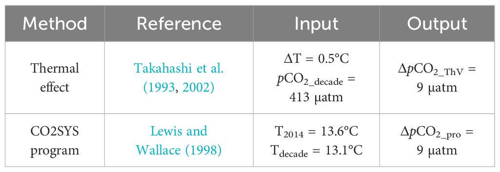
Table 2 Two methods to explore the quantitative impact of temperature changes on partial pressure of CO₂ in the sea surface (pCO₂).

The average pCO₂ from 2009 to 2018 (pCO_{2_decade}) is 413 µatm. And the average pCO₂ in 2014 (pCO_{2_2014}) is 421 µatm, so the actual ΔpCO₂ change (ΔpCO_{2_AV}) is 8 µatm. Meanwhile, the average temperature in 2014 is 0.5° higher than the decade’s average. This provides the values for the two parameters on the right side of Equation 4, specifically: ΔT = 0.5°C, pCO_{2_decade} = 413 µatm. Inserting these values into the Equation 4 mentioned above, the theoretical ΔpCO₂ value (ΔpCO_{2_ThV}) due to the warming effect is calculated to be 9 µatm (Table 2). And this value is very close to ΔpCO_{2_pro} = 9 µatm calculated through the CO2SYS program. Furthermore, the changes in pCO₂ derived through both methods, ΔpCO_{2_ThV} and ΔpCO_{2_pro}, both closely match the ΔpCO_{2_AV}. This indicates that the relatively strong source in 2014 was dominated by the effect of rising temperatures. Specifically, the average temperature in 2014 was 0.5° higher than the multi-year mean (Figure 7A), leading to an increase of 0.9 mmol m^–2 d^–1 in FCO₂ compared to the multi-year average (Figure 7B).

4.3 Mechanism analysis of the relatively strong sink of air-sea CO₂ flux in the Northern Yellow Sea in 2016

The analysis in section 4.1 reveals that the relatively low FCO₂ in 2016 is mainly influenced by non-thermal effects. The anomalously low DIC is the primary factor for the relatively low FCO₂ in 2016. Previous studies have shown the significant role of DIC in regulating the interannual variability of FCO₂ (Le Quéré et al., 2000; Lovenduski et al., 2007; Doney et al., 2009; Omar et al., 2019; Menviel et al., 2023). Wang and Zhai (2021) suggested that the seasonal variations of sea surface pCO₂ are influenced by the surface DIC concentration. And because the changes in DIC concentration are influenced by both biological processes (net community production) and physical processes (advection, vertical mixing, air-sea CO₂ exchange). Therefore, in order to further investigate the main reasons for the abnormal change in DIC concentration, we analyze the interannual variations of the DIC budget components in the NYS upper mixed layer based on Equation 1, as shown in Figure 8.

Figure 8

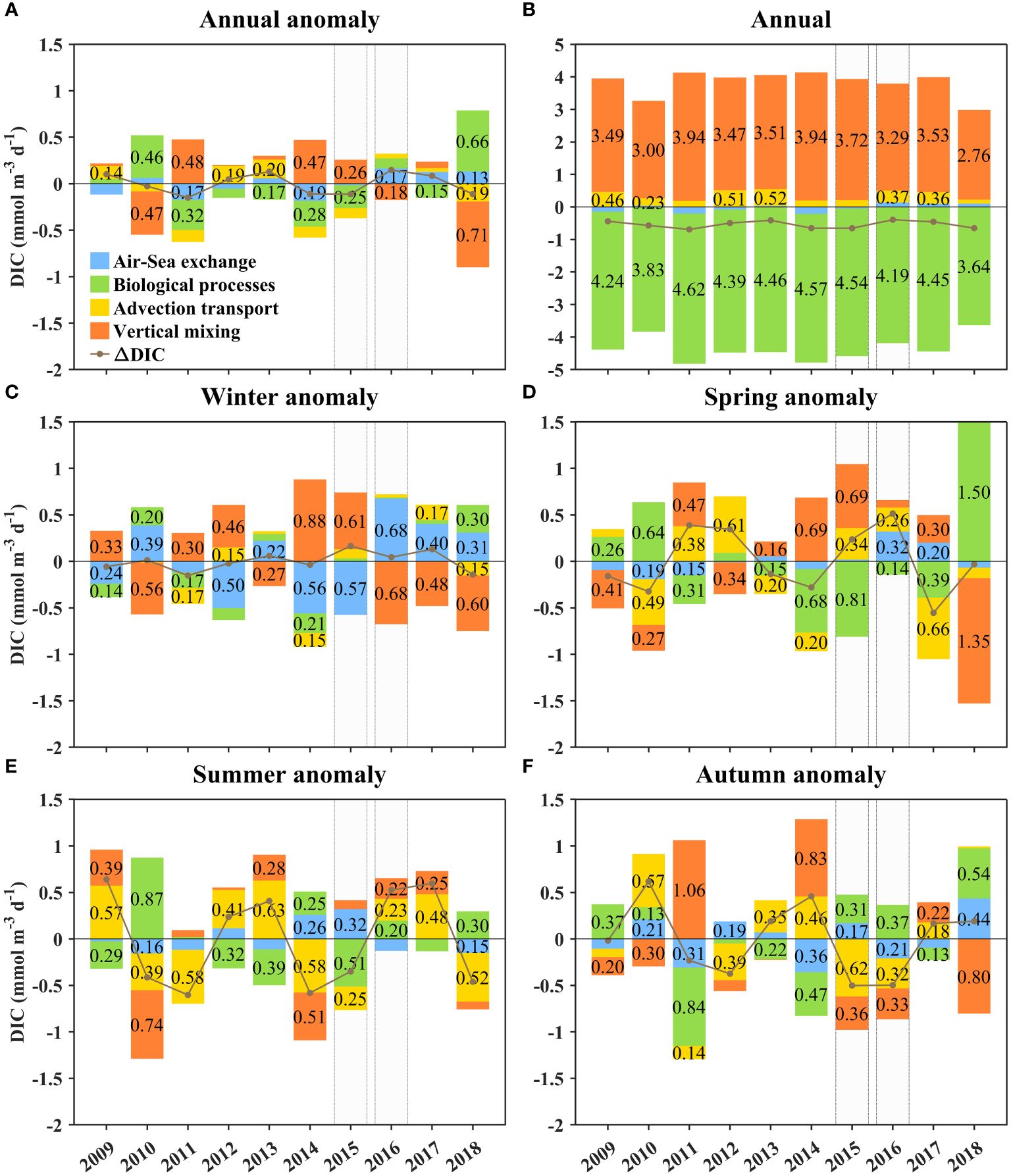
Figure 8 The interannual variations of dissolved inorganic carbon (DIC) budget components in the upper mixed layer of the Northern Yellow Sea (NYS) from 2009 to 2018 (A) the annual average anomalies, (B) the annual average, (D, E) the anomalies in winter, spring, summer, and autumn, respectively. The blue, green, yellow, and orange blocks in the figure represent the sea-air exchange, net biological processes, advection transport, and vertical mixing, respectively. In (A, C–F) positive values indicate positive anomalies, and negative values indicate negative anomalies. The gray-black dots represent the anomalies in the net rate of DIC change, its positive and negative values show deviations from their respective multi-year average rates of net change. While in (B) positive values represent positive contributions, and negative values represent negative contributions. The gray-black dots represent the annual net rate of DIC change.

The upper mixed layer is the top of the seasonal thermocline, where the water properties are relatively homogeneous. The exchange of energy, momentum, and matter between the ocean and the atmosphere primarily occurs within the upper mixed layer (Sun et al., 2007). Thus, selecting the ocean upper mixed layer to investigate the mechanisms of FCO₂ variability is of great significance. Figure 9 shows the minimum value, average value, and standard deviation of the shallowest mixed layer depth from 2009 to 2018. It can be seen from Figure 9A that the minimum value of the shallowest mixed layer depth in the center of NYS over multiple years is approximately 10 m, and the multi-year average of the shallowest mixed layer depth is slightly greater than this value (Figure 9B). The multi-year standard deviation is less than 4 m (Figure 9C). To avoid the influence of stratification depth and other, and to ensure consistency in the selected water column for the budget analysis, we chose the water within the minimum value of shallowest upper mixed layer depth in Figure 9A as the upper mixed layer.

Figure 9

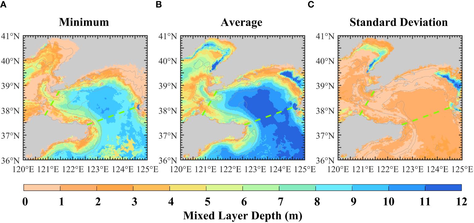
Figure 9 Spatial distribution of shallowest mixed layer depths in the Northern Yellow Sea (NYS), (A) the minimum value of the shallowest mixed layer depth from 2009 to 2018, (B) the average value of the shallowest mixed layer depth from 2009 to 2018, (C) The standard deviation of the shallowest mixed layer depth from 2009 to 2018. The two green dashed lines represent the NYS boundary.

Additionally, Figure 8 shows the interannual variations of each component of the DIC budget in the upper mixed layer of the NYS from 2009 to 2018. To further illustrate, Figure 8B represents the interannual variations of the annual DIC budget, while the remaining five subplots show the interannual variations of the DIC budget anomalies (Figures 8A, C–E). The anomalies for each component are calculated by subtracting the average value of that component respectively. The purpose of this approach is to highlight which component’s abnormal change is the main factor for driving the interannual changes. The annual results show that the biological processes generally exhibit a negative contribution to DIC concentration, while vertical mixing commonly exhibits a positive contribution to DIC concentration (Figure 8B). It should be noted that the effect of calcium carbonate formation and dissolution is not included in the biological processes of the current model, because of limited information on the abundance and distribution of planktonic calcifying organisms. Future modeling efforts will consider additional groups of organisms.

Below, we will conduct a further analysis of the anomaly results (Figures 8A, C–E). Figure 7B shows that the DIC concentration in 2016 was the lowest in the multi-year period. However, based on the annual average anomaly results, it can be observed that the net rate of DIC change within the upper mixed layer of the NYS in 2016 exhibited a positive anomaly compared to the multi-year average, indicating a net increase in DIC replenishment compared to the multi-year average (Figure 8A). This suggests that the abnormally low DIC concentration in 2016 is not caused by interannual variations but rather stems from an initially low DIC concentration in the winter of 2016. Figure 7B also illustrates the lower winter DIC levels in 2016. Furthermore, Figure 7B reveal that before the winter of 2016, the DIC concentration in the summer and autumn of 2015 is already unusually low compared to the multi-year average. According to the seasonal cycle adopted in this study (winter-spring-summer-autumn), it can be concluded that the low initial DIC concentration in winter 2016 is influenced by the DIC variation in 2015. The DIC concentration in the initial winter of 2015 is higher than the multi-year winter average (Figure 7B). While the net rate of DIC change within the upper mixed layer of the NYS in 2015 exhibits a negative anomaly compared to the multi-year average (Figure 8A), indicating an overall net decrease in DIC concentration in 2015. Therefore, the abnormally low initial DIC concentration in 2016 results from the processes occurring in 2015. In summary, an analysis of the interannual variations in DIC budget anomalies reveals the abnormally low DIC concentration in 2016 is not influenced by processes within that year, but instead is due to its abnormally low initial concentration. This initial state in turn is affected by the net community production in the summer and the advective processes in the autumn of 2015. Further analysis follows.

4.4 The mechanisms of abnormally low initial DIC concentration in 2016

According to the analysis results from the previous section, the abnormally low initial DIC concentration in the NYS in 2016 can be attributed to the decrease in DIC during 2015. Combining Figures 8C–E, it can be observed that the net rate of DIC concentration change during the winter and spring of 2015 is positively anomalous compared to the multi-year average, while during the summer and autumn, it is negatively anomalous. This indicates that the anomalous decrease in DIC is primarily controlled by processes during the summer and autumn of 2015. It is worth noting that the net rate of change in DIC during the summer net community production in 2015 shows the most pronounced relative change compared to the multi-year summer average, with a difference of –0.5 mmol m^–3 d^–1 (Figure 8E). Furthermore, compared to other components, the net rate of change in DIC during the autumn advection processes in 2015 shows the most distinct change relative to the multi-year autumn average, with a difference of –0.6 mmol m^–3 d^–1 (Figure 8F). To further investigate the influence of these two processes, the primary production, water fluxes, and DIC fluxes in and out of the NYS in 2015 are analyzed (Table 3; Figure 10).

Table 3

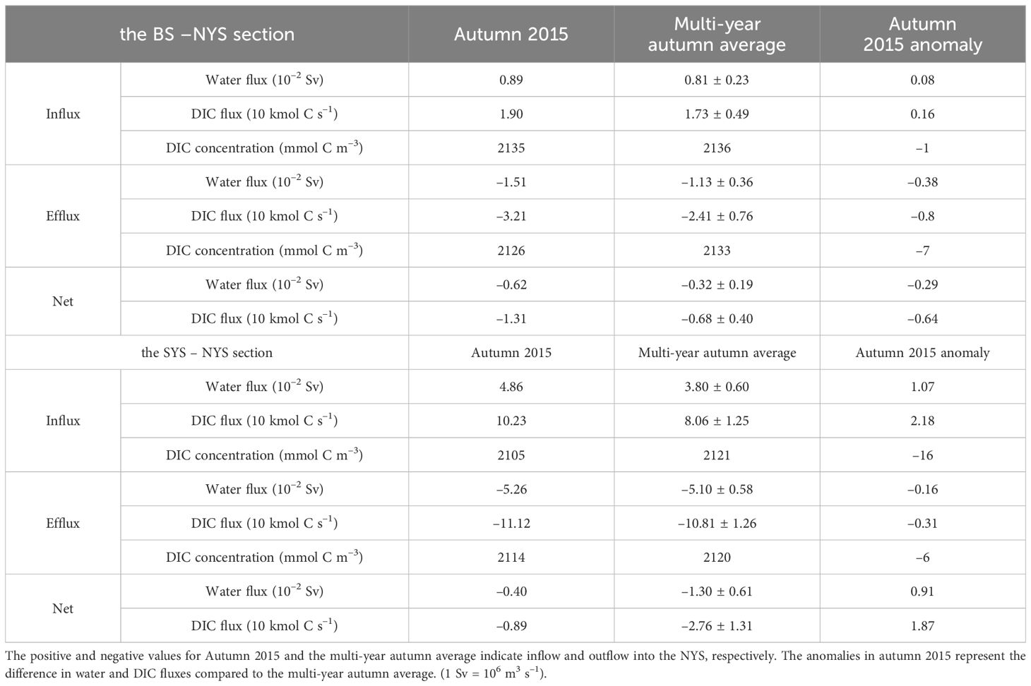
Table 3 Water flux and dissolved inorganic carbon (DIC) flux in the upper mixed layer on the Bohai Sea (BS) – Northern Yellow Sea (NYS) section and the Southern Yellow Sea (SYS) – NYS section.

Figure 10

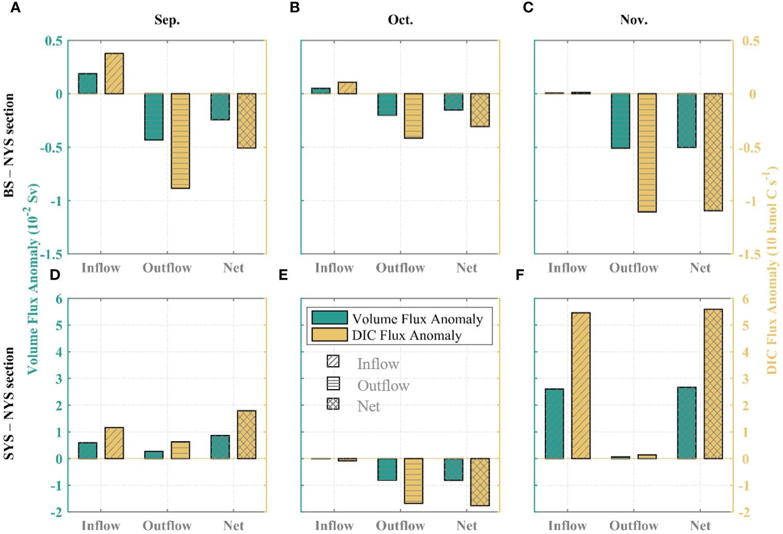
Figure 10 Anomalies of water flux (10^–2 Sv; 1 Sv = 10⁶ m³ s^–1) and dissolved inorganic carbon (DIC) flux (10 kmol C s^–1) in each month of autumn 2015, including inflow, outflow, and net flux anomalies. (A–C) The Bohai Sea (BS) – Northern Yellow Sea (NYS) section, (D–F) the Southern Yellow Sea (SYS) – NYS section. (A, D) September anomalies, (B, E) October anomalies, (C, F) November anomalies.

First, to examine the impact of the summer net community production in 2015, the interannual variations of primary production anomalies in the NYS from 2009 to 2018 (Figure 11) are analyzed using model results. From Figure 11, it can be seen that the average primary production anomaly in 2015 is high, and the primary production during the summer of 2015 is the highest among summers in multi-year. Specifically, during the summer of 2015, the primary production is 0.7 mmol m^–3 d^–1 higher than the multi-year average for summers. This will lead to a higher consumption of DIC due to biological processes, consistent with the understanding of the lower DIC concentration during the summer of 2015 (Figure 7). Furthermore, Wang and Zhai (2021) also indicated that in August 2015, the NYS exhibited abnormally high DO saturation and low CO₂ fugacity compared to other survey years. Therefore, the higher level of phytoplankton primary production during the summer of 2015 results in increased DIC consumption, contributing to the lower DIC concentration in the NYS during that season.

Figure 11

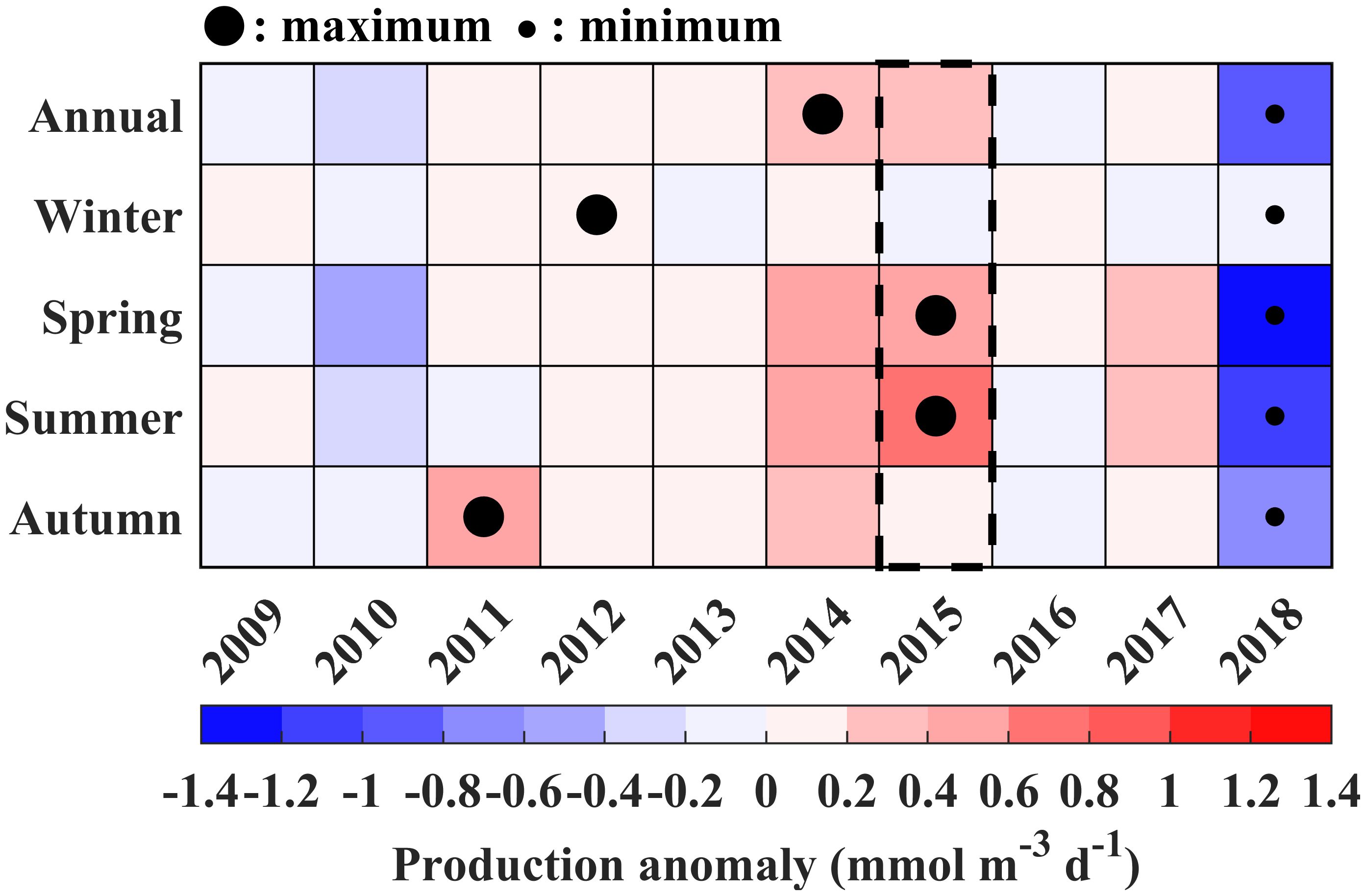
Figure 11 Interannual variations of the primary production anomalies in the Northern Yellow Sea (NYS) from 2009 to 2018. Large black solid dots represent the multi-year maximum values, while small black solid dots represent the multi-year minimum values.

To further explore the impact of advection processes, the BS – NYS section and the SYS – NYS section (as shown in Figure 1) are selected for the analysis of water fluxes and DIC fluxes (Table 3; Figure 10). To maintain consistency with the previous budget analysis, the flux calculation is confined to the upper mixed layer. The water flux is calculated by multiplying the grid velocity by the grid cross-sectional area, and then summing up the entire section, while the DIC flux is calculated using the same method, but it requires multiplying the DIC concentration of each grid section. The results show that in the BS – NYS section, the water and DIC fluxes during the autumn of 2015 exhibit a net outflow anomaly compared to the multi-year autumn average, with increases of 33.63% and 33.20% in the outflow water and DIC fluxes, respectively (Table 3). In contrast, in the SYS-NYS section, the autumn of 2015 exhibits a net inflow anomaly compared to the multi-year autumn average. Although the DIC flux inflow increases by 27.05% compared to the multi-year average, it is mainly due to the inflow of more low-concentration-DIC water. The water volume increases by 28.15% relative to the multi-year average, while the DIC concentration decreases by 16 mmol C m^–3 compared to the average (Table 3). Furthermore, as indicated by Figure 2 and survey results (Wang and Zhai, 2021), the autumn DIC concentration in the BS and the NYS generally exhibited a north-high and south-low spatial distribution pattern. The enhanced water transport from the SYS to the NYS introduces more low-concentration-DIC water. These results indicate that the abnormally high DIC reduction in the autumn advection process of 2015 is mainly due to the increased influx of low-concentration-DIC water from the SYS into the NYS and the increased outflow from the NYS into the BS.

To further investigate the cause for the anomalous fluxes, an analysis of the average flow field for the autumn of 2015 is conducted, revealing no obvious anomalies in the flow field. When specifically analyzing the inflow, outflow, and net flux anomalies of water and DIC fluxes in each month of autumn 2015 (Figure 10), it is found that November is the key month responsible for the pronounced reduction in the advection processes and the high DIC anomalies. In both the BS – NYS section and the SYS – NYS section, the net flux anomalies of water and DIC in November are markedly higher than in September and October. In the BS – NYS section, the net flux anomalies of water and DIC in November are –0.5 × 10^–2 Sv and –1.09 × 10 kmol C s^–1, respectively. In the SYS – NYS section, the net flux anomalies of water and DIC in November were 2.67 × 10^–2 Sv and 5.59 × 10 kmol C s^–1, respectively. This indicates that the advection in November 2015 plays a key role in reducing the DIC concentration in the NYS during the autumn.

Wan et al. (2015) showed that strong wind events can evidently affect the circulation and water exchange capacity in the BS (Wan et al., 2015). Figures 12A, B indicate that in the BS – NYS section, wind stress abnormally intensifies, and the wind direction shifts towards the northeast. Due to the Coriolis force and Ekman transport, the flow field anomaly at the section shifts westward, leading to an increase in water flowing from the NYS to the BS. In the SYS – NYS section, there is an eastward shift in wind stress anomalies, causing the flow field anomalies to shift northward. The flow from the SYS to the NYS obviously increased, leading to an increased influx of low-concentration-DIC water from the SYS into the NYS. Li et al. (2015) also pointed out that strong wind events increased the water exchange between the Bohai and Yellow Seas, leading to a deeper intrusion of YS water into the BS.

Figure 12

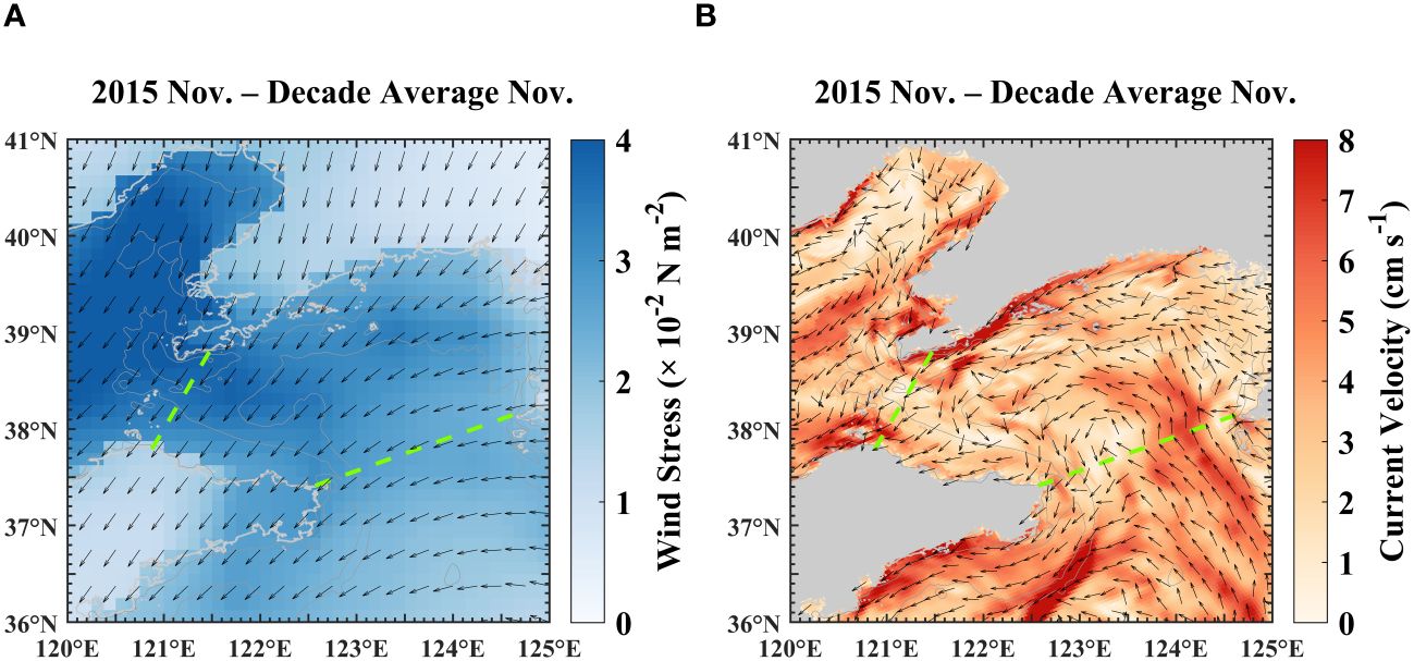
Figure 12 (A) Wind stress anomalies in November 2015, (B) Current field anomalies in November 2015. The green dashed lines represent the Bohai Sea (BS) – Northern Yellow Sea (NYS) section and the Southern Yellow Sea (SYS) – NYS section in this study.

In conclusion, net community production in the summer of 2015 and advection processes in the autumn combine to result in abnormally low initial values of DIC concentration in 2016. The anomalous decrease in DIC during the summer of 2015 is mainly attributed to the abnormally high level of phytoplankton primary production. The impact of the advection processes in the autumn of 2015 is primarily reflected in the strong northeasterly wind event and the anomaly of the flow field in November 2015, which causes a deeper intrusion of YS water into the BS and an enhanced flow from the SYS into the NYS. The DIC concentration exhibits a spatial distribution that gradually increases from south to north. These ultimately lead to higher DIC flux from the NYS into the BS in the upper mixed layer and increase the inflow of low-concentration-DIC water from the SYS into the NYS. All of these finally lead to the abnormally low initial DIC concentration in 2016.

5 Conclusions

The continental shelf seas play a pivotal role in the air-sea CO₂ exchange. However, due to the complex spatio-temporal variations and sparse field observations, there is a lack of understanding of the interannual variability of FCO₂. In this study, the hindcast simulation of the 3-D physical-biogeochemical-carbon cycle coupled model is used to analyze the underlying mechanism behind the abnormal carbon source/sink pattern in the NYS. The simulation results reveal the significant interannual variability in the NYS’s FCO₂. Specifically, the NYS acts as an abnormalCO₂ source in 2014 and transitions into an anomalous sink in 2016. The relatively strong CO₂ source in 2014 is attributed to abnormally high temperatures, while the relatively strong CO₂ sink in 2016 is due to the abnormally low DIC concentration. Further investigation reveals that the cause of the low DIC concentration in the NYS in 2016 is the initial low DIC concentration. The low initial DIC concentration results from the combined effects of high primary production in the summer of 2015 and advection processes in the autumn of 2016. Net community production increase DIC consumption due to abnormally high primary production in the summer of 2015. Advection processes reduce more DIC due to the strong northeasterly wind event and anomalous current patterns. These further increase higher DIC flux from the NYS into the BS in the upper mixed layer and increase the inflow of low-concentration-DIC water from the SYS into the NYS. This study deepens the understanding of the interannual variability of the FCO₂ in the NYS. It also reveals that physical and biological processes are crucial not only for seasonal variability but also for interannual variability in sea-air CO₂ source and sink dynamics. This is of great significance for better assessing the carbon sink capacity of the continental shelf seas under future climate change.

Data availability statement

Publicly available datasets were analyzed in this study. This data can be found here:

https://figshare.com/articles/dataset/Mapping_dataset_of_dissolved_oxygen_and_carbonate_system_comparing_seasonal_subsurface_deoxygenation_and_acidification_in_the_Yellow_Sea_and_northern_East_China_Sea_in_2017-2018/12630335

https://figshare.com/articles/dataset/Mapping_dataset_of_dissolved_oxygen_and_carbonate_system_showing_autumnal_subsurface_acidification_in_the_central_North_Yellow_Sea_in_2017/12630212

https://figshare.com/articles/dataset/Dissolved_oxygen_and_carbonate_system_in_a_southern_nearshore_marine_aquaculture_area_in_the_North_Yellow_Sea_in_May_June_July_August_and_September_2017/12630101

https://figshare.com/articles/dataset/Sea_surface_carbonate_mapping_data_of_10_cruises_in_the_Yellow_Sea_during_2011_to_2018/11962161

https://figshare.com/articles/dataset/Dataset_of_dissolved_oxygen_and_carbonate_parameters_supporting_the_study_entitiled_as_Emergence_of_summertime_hypoxia_and_concurrent_carbonate_mineral_suppression_in_the_central_Bohai_Sea_China_/9248822.

Author contributions

JL: Writing – original draft, Writing – review & editing. HN: Writing – review & editing. JS: Writing – review & editing. HW: Writing – review & editing. GG: Writing – review & editing. HZ: Writing – review & editing.

Funding

The author(s) declare financial support was received for the research, authorship, and/or publication of this article. This study was supported by the National Natural Science Foundation of China (Grant No. 42141020) and the National Key Research and Development Program of China (2023YFC3107702). Most of the sampling surveys were supported by the National Natural Science Foundation of China (NSFC) via Open Ship‐time Sharing Projects in the Bohai and Yellow Seas.

Acknowledgments

We would like to thank the organizations that provided the data used in this work, including the World Ocean Atlas 2013 (WOA13), the Hybrid Coordinate Ocean Model (HYCOM), the European Centre for Medium-Range Weather Forecasts (ECMWF), the Copernicus Marine Environment Monitoring Service (CMEMS), the Global Monitoring Laboratory of the National Oceanic and Atmospheric Administration (NOAA). We are grateful to the ROMS-CoSiNE development team for providing the state-of-the-art model. Finally, we thank the editor and reviewers for their constructive suggestions on our work.

Conflict of interest

The authors declare that the research was conducted in the absence of any commercial or financial relationships that could be construed as a potential conflict of interest.

Publisher’s note

All claims expressed in this article are solely those of the authors and do not necessarily represent those of their affiliated organizations, or those of the publisher, the editors and the reviewers. Any product that may be evaluated in this article, or claim that may be made by its manufacturer, is not guaranteed or endorsed by the publisher.

References

Bao X., Li N., Yao Z., Wu D. (2009). Seasonal variation characteristics of temperature and salinity of the north yellow sea. Periodical Ocean Univ. China 39, 553–562. doi: 10.16441/j.cnki.hdxb.2009.04.002

CrossRef Full Text | Google Scholar

Bauer J. E., Cai W.-J., Raymond P. A., Bianchi T. S., Hopkinson C. S., Regnier P. A. G. (2013). The changing carbon cycle of the coastal ocean. Nature 504, 61–70. doi: 10.1038/nature12857

PubMed Abstract | CrossRef Full Text | Google Scholar

Burt W. J., Thomas H., Hagens M., Pätsch J., Clargo N. M., Salt L. A., et al. (2016). Carbon sources in the North Sea evaluated by means of radium and stable carbon isotope tracers. Limnology Oceanography 61, 666–683. doi: 10.1002/lno.10243

CrossRef Full Text | Google Scholar

Chai F., Dugdale R. C., Peng T.-H., Wilkerson F. P., Barber R. T. (2002). One-dimensional ecosystem model of the equatorial Pacific upwelling system. Part I: model development and silicon and nitrogen cycle. Deep Sea Res. Part II: Topical Stud. Oceanography 49, 2713–2745. doi: 10.1016/S0967-0645(02)00055-3

CrossRef Full Text | Google Scholar

Dai M., Su J., Zhao Y., Hofmann E. E., Cao Z., Cai W.-J., et al. (2022). Carbon fluxes in the coastal ocean: synthesis, boundary processes, and future trends. Annu. Rev. Of Earth And Planetary Sci. 50, 593–626. doi: 10.1146/annurev-earth-032320-090746

CrossRef Full Text | Google Scholar

Doney S. C., Lima I., Feely R. A., Glover D. M., Lindsay K., Mahowald N., et al. (2009). Mechanisms governing interannual variability in upper-ocean inorganic carbon system and air-sea CO₂ fluxes: Physical climate and atmospheric dust. Deep Sea Res. Part II: Topical Stud. Oceanography 56, 640–655. doi: 10.1016/j.dsr2.2008.12.006

CrossRef Full Text | Google Scholar

Friedlingstein P., O’Sullivan M., Jones M. W., Andrew R. M., Bakker D. C. E., Hauck J., et al. (2023). Global carbon budget 2023. Earth System Sci. Data 15, 5301–5369. doi: 10.5194/essd-15-5301-2023

CrossRef Full Text | Google Scholar

Gray A. R., Johnson K. S., Bushinsky S. M., Riser S. C., Russell J. L., Talley L. D., et al. (2018). Autonomous biogeochemical floats detect significant carbon dioxide outgassing in the high-latitude southern ocean. Geophysical Res. Lett. 45, 9049–9057. doi: 10.1029/2018GL078013

CrossRef Full Text | Google Scholar

Gruber N. (2015). Carbon at the coastal interface. Nature 517, 148–149. doi: 10.1038/nature14082

PubMed Abstract | CrossRef Full Text | Google Scholar

Gruber N., Clement D., Carter B. R., Feely R. A., Van Heuven S., Hoppema M., et al. (2019). The oceanic sink for anthropogenic CO₂ from 1994 to 2007. Science 363, 1193–1199. doi: 10.1126/science.aau5153

PubMed Abstract | CrossRef Full Text | Google Scholar

Guo S., Zhang H., Wei H., Zhao L. (2022). Summer high temperature phenomenon and its mechanism in the Bohai Sea from 2013 to 2019 [in Chinese with English abstract]. Oceanologia Et Limnologia Sin. 53, 269–277. doi: 10.11693/hyhz20210900208

CrossRef Full Text | Google Scholar

Hu X., Nuttall M. F., Wang H., Yao H., Staryk C. J., McCutcheon M. R., et al. (2018). Seasonal variability of carbonate chemistry and decadal changes in waters of a marine sanctuary in the Northwestern Gulf of Mexico. Mar. Chem. 205, 16–28. doi: 10.1016/j.marchem.2018.07.006

CrossRef Full Text | Google Scholar

Jiang Z., Hydes D. J., Tyrrell T., Hartman S. E., Hartman M. C., Dumousseaud C., et al. (2013). Key controls on the seasonal and interannual variations of the carbonate system and air-sea CO ₂ flux in the Northeast Atlantic (Bay of Biscay). J. Geophysical Research: Oceans 118, 785–800. doi: 10.1002/jgrc.20087

CrossRef Full Text | Google Scholar

Kealoha A. K., Shamberger K. E. F., DiMarco S. F., Thyng K. M., Hetland R. D., Manzello D. P., et al. (2020). Surface water CO₂ variability in the gulf of Mexico, (1996–2017). Sci. Rep. 10, 12279. doi: 10.1038/s41598-020-68924-0

PubMed Abstract | CrossRef Full Text | Google Scholar

Keenan T. F., Davidson E., Moffat A. M., Munger W., Richardson A. D. (2012). Using model-data fusion to interpret past trends, and quantify uncertainties in future projections, of terrestrial ecosystem carbon cycling. Global Change Biol. 18, 2555–2569. doi: 10.1111/j.1365-2486.2012.02684.x

CrossRef Full Text | Google Scholar

Ko Y. H., Seok M.-W., Jeong J.-Y., Noh J.-H., Jeong J., Mo A., et al. (2022). Monthly and seasonal variations in the surface carbonate system and air-sea CO₂ flux of the Yellow Sea. Mar. pollut. Bull. 181, 113822. doi: 10.1016/j.marpolbul.2022.113822

PubMed Abstract | CrossRef Full Text | Google Scholar

Laruelle G. G., Cai W.-J., Hu X., Gruber N., Mackenzie F. T., Regnier P. (2018). Continental shelves as a variable but increasing global sink for atmospheric carbon dioxide. Nat. Commun. 9, 454. doi: 10.1038/s41467-017-02738-z

PubMed Abstract | CrossRef Full Text | Google Scholar

Laruelle G. G., Dürr H. H., Lauerwald R., Hartmann J., Slomp C. P., Goossens N., et al. (2013). Global multi-scale segmentation of continental and coastal waters from the watersheds to the continental margins. Hydrology Earth System Sci. 17, 2029–2051. doi: 10.5194/hess-17-2029-2013

CrossRef Full Text | Google Scholar

Laruelle G. G., Lauerwald R., Pfeil B., Regnier P. (2014). Regionalized global budget of the CO₂ exchange at the air-water interface in continental shelf seas. Global Biogeochemical Cycles 28, 1199–1214. doi: 10.1002/2014GB004832

CrossRef Full Text | Google Scholar

Lauvset S. K., Tjiputra J., Muri H. (2017). Climate engineering and the ocean: effects on biogeochemistry and primary production. Biogeosciences 14, 5675–5691. doi: 10.5194/bg-14-5675-2017

CrossRef Full Text | Google Scholar

Legge O. J., Bakker D. C. E., Johnson M. T., Meredith M. P., Venables H. J., Brown P. J., et al. (2015). The seasonal cycle of ocean-atmosphere CO₂ flux in Ryder Bay, west Antarctic Peninsula. Geophysical Res. Lett. 42, 2934–2942. doi: 10.1002/2015GL063796

CrossRef Full Text | Google Scholar

Legge O. J., Bakker D. C. E., Meredith M. P., Venables H. J., Brown P. J., Jones E. M., et al. (2017). The seasonal cycle of carbonate system processes in Ryder Bay, West Antarctic Peninsula. Deep Sea Res. Part II: Topical Stud. Oceanography 139, 167–180. doi: 10.1016/j.dsr2.2016.11.006

CrossRef Full Text | Google Scholar

Le Quéré C., Orr J. C., Monfray P., Aumont O., Madec G. (2000). Interannual variability of the oceanic sink of CO₂ from 1979 through 1997. Global Biogeochemical Cycles 14, 1247–1265. doi: 10.1029/1999GB900049

CrossRef Full Text | Google Scholar

Lewis E., Wallace D. (1998). Program developed for CO₂ system calculations. in ORNL/CDIAC-105, Carbon Dioxide Information Analysis Center (Oak Ridge National Laboratory). Available at: https://www.ncei.noaa.gov/access/ocean-carbon-acidification-data-system/oceans/CO2SYS/co2rprt.html.

Google Scholar

Li J., Song J., Mo L., Wang Y., Li D., Wang G. (2015). Characteristics of Sea water exchange between Bohai Sea and Yellow Sea under the effect of high wind in winter. Mar. Sci. Bull. 34, 647–656. doi: 10.11840/j.issn.1001–6392.2015.06.007

CrossRef Full Text | Google Scholar

Li Z., Wei H., Zhang H., Zhao H., Zheng N., Song G. (2021). The interannual difference in summer bottom oxygen deficiency in Bohai Sea. Oceanologia Et Limnologia Sin. 52, 601–613. doi: 10.11693/hyhz20200800227

CrossRef Full Text | Google Scholar

Li C., Zhai W. (2021). Mechanism-based deduction of subsurface aragonite saturation state in a semi-enclosed and seasonally stratified coastal sea. Mar. Chem. 232, 103958. doi: 10.1016/j.marchem.2021.103958

CrossRef Full Text | Google Scholar

Lovenduski N. S., Gruber N., Doney S. C., Lima I. D. (2007). Enhanced CO₂ outgassing in the Southern Ocean from a positive phase of the Southern Annular Mode. Global Biogeochemical Cycles 21, GB2026. doi: 10.1029/2006GB002900

CrossRef Full Text | Google Scholar

Luo C., Nie H., Zhang H. (2019). Spatial variability of parameter sensitivity in the ecosystem simulation of the Bohai Sea and Yellow Sea [in Chinese with English abstract]. Haiyang Xuebao 41, 85–96. doi: 10.3969/j.issn.0253–4193.2019.08.008

CrossRef Full Text | Google Scholar

Menviel L. C., Spence P., Kiss A. E., Chamberlain M. A., Hayashida H., England M. H., et al. (2023). Enhanced Southern Ocean CO₂ outgassing as a result of stronger and poleward shifted southern hemispheric westerlies. Biogeosciences 20, 4413–4431. doi: 10.5194/bg-20-4413-2023

CrossRef Full Text | Google Scholar

Omar A. M., Thomas H., Olsen A., Becker M., Skjelvan I., Reverdin G. (2019). Trends of ocean acidification and pCO₂ in the northern north sea 2003–2015. JGR Biogeosciences 124, 3088–3103. doi: 10.1029/2018JG004992

CrossRef Full Text | Google Scholar

Prowe A. E. F., Thomas H., Pätsch J., Kühn W., Bozec Y., Schiettecatte L.-S., et al. (2009). Mechanisms controlling the air-sea CO₂ flux in the North Sea. Continental Shelf Res. 29, 1801–1808. doi: 10.1016/j.csr.2009.06.003

CrossRef Full Text | Google Scholar

Radach G., Moll A. (2006). “Review of three-dimensional ecological modelling related to the North Sea shelf system. Part II: Model validation and data needs,” in Oceanography and marine biology: An annual review, vol. 44 . Eds. Gibson R. N., Atkinson R. J. A., Gordon J. D. M. (Boca Raton, FL: CRC Press, Taylor and Francis Group), 1–60. doi: 10.1201/9781420006391

CrossRef Full Text | Google Scholar

Ren H., Zhan J. (2005). A numerical study on the seasonal variability of the Yellow Sea cold water mass and the related dynamics. J. Hydrodynamics 20, 887–896. doi: 10.16076/j.cnki.cjhd.2005.s1.012

CrossRef Full Text | Google Scholar

Robbins L. L., Daly K. L., Barbero L., Wanninkhof R., He R., Zong H., et al. (2018). Spatial and temporal variability of pCO₂, carbon fluxes, and saturation state on the West Florida shelf. J. Geophysical Research: Oceans 123, 6174–6188. doi: 10.1029/2018JC014195

CrossRef Full Text | Google Scholar

Schiettecatte L.-S., Thomas H., Bozec Y., Borges A. V. (2007). High temporal coverage of carbon dioxide measurements in the Southern Bight of the North Sea. Mar. Chem. 106, 161–173. doi: 10.1016/j.marchem.2007.01.001

CrossRef Full Text | Google Scholar

Shchepetkin A. F., McWilliams J. C. (2005). The regional oceanic modeling system (ROMS): a split-explicit, free-surface, topography-following-coordinate oceanic model. Ocean Model. 9, 347–404. doi: 10.1016/j.ocemod.2004.08.002

CrossRef Full Text | Google Scholar

Shi J.-H., Gao H.-W., Zhang J., Tan S.-C., Ren J.-L., Liu C.-G., et al. (2012). Examination of causative link between a spring bloom and dry/wet deposition of Asian dust in the Yellow Sea, China. J. Geophysical Research: Atmospheres 117, D17304. doi: 10.1029/2012JD017983

CrossRef Full Text | Google Scholar

Song M., Zhang L., Jiang C. (2007). The distribution of partial pressure of CO₂ and its maintaining mechanism: vertical mixing versus biological activity in the yellow sea in early spring. Periodical Ocean Univ. China 37, 67–72. doi: 10.16441/j.cnki.hdxb.2007.s1.010

CrossRef Full Text | Google Scholar

State Oceanic Administration, C. (2010). Bulletin of marine environmental status of China in 2009. Available at: https://nmdis.org.cn/hygb/zghyhjzlgb/2009nzghyhjzkgb/.

Google Scholar

State Oceanic Administration, C. (2013). Bulletin of marine environmental status of China in 2012. Available at: https://nmdis.org.cn/hygb/zghyhjzlgb/2012nzghyhjzkgb/.

Google Scholar

Sun C., Liu Q., Jia Y. (2007). Annual and interannual variations of the mixed layer in the South China sea. Periodical Ocean Univ. China 37, 197–203. doi: 10.16441/j.cnki.hdxb.2007.02.004

CrossRef Full Text | Google Scholar

Takahashi T., Olafsson J., Goddard J. G., Chipman D. W., Sutherland S. C. (1993). Seasonal variation of CO₂ and nutrients in the high-latitude surface oceans: A comparative study. Global Biogeochemical Cycles 7, 843–878. doi: 10.1029/93GB02263

CrossRef Full Text | Google Scholar

Takahashi T., Sutherland S. C., Sweeney C., Poisson A., Metzl N., Tilbrook B., et al. (2002). Global sea-air CO₂ flux based on climatological surface ocean pCO₂, and seasonal biological and temperature effects. Deep Sea Res. Part II: Topical Stud. Oceanography 49, 1601–1622. doi: 10.1016/S0967-0645(02)00003-6

CrossRef Full Text | Google Scholar

Tan S.-C., Wang H. (2014). The transport and deposition of dust and its impact on phytoplankton growth in the Yellow Sea. Atmospheric Environ. 99, 491–499. doi: 10.1016/j.atmosenv.2014.10.016

CrossRef Full Text | Google Scholar

Thomas H., Bozec Y., Elkalay K., De Baar H. J. W. (2004). Enhanced open ocean storage of CO₂ from shelf sea pumping. Science 304, 1005–1008. doi: 10.1126/science.1095491

PubMed Abstract | CrossRef Full Text | Google Scholar

Tsunogai S., Watanabe S., Nakamura J., Ono T., Sato T. (1997). A preliminary study of carbon system in the East China Sea. J. Oceanography 53, 9–17. doi: 10.1007/BF02700744

CrossRef Full Text | Google Scholar

Tsunogai S., Watanabe S., Sato T. (1999). Is there a “continental shelf pump” for the absorption of atmospheric CO₂? Tellus B: Chem. Phys. Meteorology 51, 701–712. doi: 10.3402/tellusb.v51i3.16468

CrossRef Full Text | Google Scholar

Wakelin S. L., Holt J. T., Blackford J. C., Allen J. I., Butenschön M., Artioli Y. (2012). Modeling the carbon fluxes of the northwest European continental shelf: Validation and budgets. J. Geophysical Research: Oceans 117, C05020. doi: 10.1029/2011JC007402

CrossRef Full Text | Google Scholar

Wan X., Ma Q., Ma W. (2015). The effect of high frequency strong winds on winter circulation and water exchange in the bohai sea by ROMS. Periodical Ocean Univ. China 45, 1–8. doi: 10.16441/j.cnki.hdxb.20140146

CrossRef Full Text | Google Scholar

Wang S., Zhai W. (2021). Regional differences in seasonal variation of air-sea CO₂ exchange in the Yellow Sea. Continental Shelf Res. 218, 104393. doi: 10.1016/j.csr.2021.104393

CrossRef Full Text | Google Scholar

Wanninkhof R. (1992). Relationship between wind speed and gas exchange over the ocean. J. Geophysical Research: Oceans 97, 7373–7382. doi: 10.1029/92JC00188

CrossRef Full Text | Google Scholar

Wanninkhof R. (2014). Relationship between wind speed and gas exchange over the ocean revisited. Limnology Oceanography: Methods 12, 351–362. doi: 10.4319/lom.2014.12.351

CrossRef Full Text | Google Scholar

Weiss R. F., Price B. A. (1980). Nitrous oxide solubility in water and seawater. Mar. Chem. 8, 347–359. doi: 10.1016/0304-4203(80)90024-9

CrossRef Full Text | Google Scholar

Xiong T., Wei Q., Zhai W., Li C., Wang S., Zhang Y., et al. (2020). Comparing subsurface seasonal deoxygenation and acidification in the yellow sea and Northern East China sea along the North-to-South latitude gradient. Front. Mar. Sci. 7. doi: 10.3389/fmars.2020.00686

CrossRef Full Text | Google Scholar

Xiu P., Chai F. (2010). Modeling the effects of size on patch dynamics of an inert tracer. Ocean Sci. 6, 413–421. doi: 10.5194/os-6-413-2010

CrossRef Full Text | Google Scholar

Xiu P., Chai F. (2011). Modeled biogeochemical responses to mesoscale eddies in the South China Sea. J. Geophysical Res. 116, C10006. doi: 10.1029/2010JC006800

CrossRef Full Text | Google Scholar

Xu X., Zang K., Zhao H., Zheng N., Huo C., Wang J. (2016). Monthly CO₂ at A4HDYD station in a productive shallow marginal sea (Yellow Sea) with a seasonal thermocline: Controlling processes. J. Mar. Syst. 159, 89–99. doi: 10.1016/j.jmarsys.2016.03.009

CrossRef Full Text | Google Scholar

Xue L., Xue M., Zhang L., Sun T., Guo Z., Wang J. (2012). Surface partial pressure of CO₂ and air-sea exchange in the northern Yellow Sea. J. Mar. Syst. 105–108, 194–206. doi: 10.1016/j.jmarsys.2012.08.006

CrossRef Full Text | Google Scholar

Xue L., Zhang L. (2011). Surface pCO₂ and air-sea CO₂ flux in the northern yellow sea during summer. Periodical Ocean Univ. China 41, 22–29. doi: 10.16441/j.cnki.hdxb.2011.12.004

CrossRef Full Text | Google Scholar

Yu S., Song Z., Bai Y., Guo X., He X., Zhai W., et al. (2023). Satellite-estimated air-sea CO₂ fluxes in the Bohai Sea, Yellow Sea, and East China Sea: Patterns and variations during 2003–2019. Sci. Total Environ. 904, 166804. doi: 10.1016/j.scitotenv.2023.166804

PubMed Abstract | CrossRef Full Text | Google Scholar

Yu F., Zhang Z., Diao X., Guo J., Tang Y.. (2006). Analysis of evolution of the Huanghai Sea cold water mass and its relationship with adjacent water masses. Acta Oceanol. Sin. 28 (5), 26–34. doi: 10.1016/S1001-8042(06)60021-3

CrossRef Full Text | Google Scholar

Zhai W. (2018). Exploring seasonal acidification in the Yellow Sea. Sci. China Earth Sci. 61, 647–658. doi: 10.1007/s11430-017-9151-4

CrossRef Full Text | Google Scholar

Zhai W., Zhao H., Su J., Liu P., Li Y., Zheng N. (2019). Emergence of summertime hypoxia and concurrent carbonate mineral suppression in the Central Bohai Sea, China. JGR Biogeosciences 124, 2768–2785. doi: 10.1029/2019JG005120

CrossRef Full Text | Google Scholar

Zhai W., Zhao H., Zheng N., Xu Y. (2012). Coastal acidification in summer bottom oxygen-depleted waters in northwestern–northern Bohai Sea from June to August in 2011. Chin Sci Bull. 57 (9), 1062–1068. doi: 10.1007/s11434-011-4949-2

CrossRef Full Text | Google Scholar

Zhai W.-D., Zheng N., Huo C., Xu Y., Zhao H.-D., Li Y.-W., et al. (2014). Subsurface pH and carbonate saturation state of aragonite on the Chinese side of the North Yellow Sea: seasonal variations and controls. Biogeosciences 11, 1103–1123. doi: 10.5194/bg-11-1103-2014

CrossRef Full Text | Google Scholar

Zhang J. (1994). Atmospheric wet deposition of nutrient elements: correlation with harmful biological blooms in northwest pacific coastal zones. Ambio 23, 464–468.

Google Scholar

Zhang L., G C., Xue L. (2009). Sea during spring distribution and controlling factors of surface seawater partial pressure of CO₂ in the northern yellow sea during autumn. Periodical Ocean Univ. China 39, 587–591. doi: 10.16441/j.cnki.hdxb.2009.04.006

CrossRef Full Text | Google Scholar

Zhang L., Wang J., Zhang Y., Xue L. (2008). Sea during spring distribution and controlling factors of surface seawater partial pressure of CO₂ in the northern yellow sea during winter. Periodical Ocean Univ. China 38, 955–960. doi: 10.16441/j.cnki.hdxb.2008.06.017

CrossRef Full Text | Google Scholar

Zhang G., Wei H., Xiao J., Zhang H., Li Z. (2020). Variation of tidal front position in LiaoDong Bay during summer 2017. Oceanologia Et Limnologia Sin. 51, 1–12. doi: 10.11693/hyhz20190600110

CrossRef Full Text | Google Scholar

Zhang H., Wei H., Zhao L., Zhao H., Guo S., Zheng N. (2022). Seasonal evolution and controlling factors of bottom oxygen depletion in the Bohai Sea. Mar. Pollut. Bull. 174, 113199. doi: 10.1016/j.marpolbul.2021.113199

PubMed Abstract | CrossRef Full Text | Google Scholar