A mesoscale eddy reconstruction method based on generative adversarial networks

Mesoscale eddies are phenomena that widely exist in the ocean and have a significant impact on the ocean’s temperature and salt structure, as well as on acoustic propagation effects. Currently, utilizing the limited data on mesoscale eddy environments for refined acoustic field reconstruction in offshore conditions at mid-to-far-ocean distances is an urgent problem that needs to be addressed. In this paper, we propose a mesoscale eddy reconstruction method (EddyGAN) based on the generative adversarial network (GAN) model which is inspired by the concept of global localization. We adopt a hybrid algorithm for eddy identification using JCOPE2M high-resolution reanalysis data and Archiving, Validation, and Interpretation of Satellite Oceanographic (AVISO) satellite altimeter data to extract mesoscale eddy sound speed profile (SSP) sample data, and then apply the EddyGAN model to train this dataset and perform mesoscale eddy acoustic field reconstruction. We also propose an evaluation method for mesoscale eddy acoustic field reconstruction that uses RMSE, SSIM, and convergence zone (CZ) accuracy based on World Ocean Atlas (WOA) climate state data completion as indicators. The reconstruction result of this model achieves an RMSE of 1.7 m/s, an SSIM of 0.77, and an average CZ accuracy of over 70%. This method better characterizes the mesoscale eddy sound field than the native GAN and other reconstruction methods, improves the accuracy of mesoscale eddy acoustic field reconstruction, and provides superior performance, offering significant reference value for mesoscale eddy reconstruction technology and subsequent ocean acoustic research.

1 Introduction

Mesoscale eddies are oceanic phenomena with spatial scales ranging from tens to hundreds of kilometers and lifetimes spanning from tens to hundreds of days (Chelton et al., 2011). They are widely distributed across the global oceans. Depending on the rotation direction, eddies can be categorized into cyclonic eddies (CEs) and anticyclonic eddies (AEs). In the Northern Hemisphere, CEs rotate counterclockwise and AEs rotate clockwise, while in the Southern Hemisphere, the opposite is true. Mesoscale eddies significantly influence local water masses, leading to pronounced differences in temperature and salinity characteristics inside and outside the eddies (Qiu and Chen, 2005). They also play a crucial role in ocean circulation, material exchange, energy transfer, and marine environmental variability (Dong et al., 2014). The Kuroshio, a strong western boundary current originating from the equatorial Pacific Ocean, is located in the region between 30°N to 40°N and 140°E to 170°E, an area often referred to as the Kuroshio Extension (KE) (Scharffenberg and Stammer, 2010) demonstrated that this region has a high density of mesoscale eddies and possesses one of the highest levels of Eddy Kinetic Energy (EKE) in the Pacific Ocean, which is also the primary research area of this paper. Itoh et al. (Itoh and Yasuda, 2010) provided a detailed account of the basic characteristics of eddies in the KE region, noting that there are more AEs with longer lifetimes to the north of the KE, and more CEs with stronger intensities to the south and near the flow axis. Overall, under the conclusion of the global observations, many composite analyses have shown that CEs usually have cold eddy centers and AEs associated with warm eddy centers (Chaigneau et al., 2011; Zhang et al., 2013, 2014). Furthermore, based on years of satellite altimeter data, the EKE of mesoscale eddies in this region exhibits strong seasonal variation, with stronger activity in summer and weaker activity in winter.

Mesoscale eddies’ characteristics induce variations in temperature and salinity within and around the eddies, significantly influencing acoustic propagation. Numerous scholars have utilized acoustic propagation models to study the effects of mesoscale eddies on acoustic transmission. Jian et al. (Jian et al., 2009) employed an analytical eddy model and two-dimensional parabolic equations to analyze acoustic transmission within the South China Sea’s anticyclonic warm-core eddies. Their theoretical calculations revealed notable acoustic field variations corresponding to shifts in the SOFAR axis’s position due to the presence of either an AE or a cyclonic eddy. Liu et al. (Liu et al., 2021) examined sound energy distributions in eddies with varying intensities through modeling and empirical data, deducing that the CZ’s position is more distant or nearer to the sound source when sound travels through cyclonic or AEs, respectively, compared to its propagation in the background current. Further, experimental studies conducted at sea have corroborated these theoretical findings. Sun et al. (Sun et al., 2023) integrated temperature and salinity measurements with concurrent acoustic field experiments within a mesoscale CE in the Northwest Pacific Ocean. They observed that cold-core eddies displace the irradiation zone toward the eddy’s perimeter, with the displacement diminishing as the sound source depth increases. Akulichev et al. (Akulichev et al., 2012) noted that the irradiation zone’s proximity to the sound source in cyclonic and AEs is closer than in the background current, highlighting mesoscale eddies’ substantial influence on horizontal sound propagation from a towed source at 100 meters depth.

Advancements in computer technology have propelled machine learning to the forefront of mesoscale eddy identification with notable successes. DuoZ et al. (Duo et al., 2019) devised a deep learning model integrating a target detection network, which, by enhancing small-sample data, yielded impressive identification outcomes. Ashkezari et al. (Ashkezari et al., 2016) explored mesoscale eddies in Peruvian waters using daily maps of geostrophic velocity anomalies along with latitudinal and longitudinal phase angle components. Lguensat et al. (Lguensat et al., 2018). leveraged deep neural networks to establish an eddy identification model founded on ‘EddyNet’, boasting a U-shaped architecture that surpassed conventional algorithms in categorical cross-entropy tests. Xu et al. (Xu et al., 2019 developed an AI algorithm for detecting oceanic eddies, employing PSPNet and vector geometry (VG)-based algorithms to refine the detection of small-scale eddies. Satellite measurements, now more prevalent than ever, provide researchers with extensive data, including sea surface height anomalies and temperatures, enabling studies on mesoscale eddy surface characteristics and their 3D reconstruction. Zhang et al. (Zhang et al., 2013) introduced a unified 3D mesoscale eddy structure by applying normalization techniques to satellite altimeter and Argo float data. Isern‐Fontanet et al. (Isern-Fontanet et al., 2008) utilized sea surface temperature anomalies to reconstruct the North Atlantic’s ocean circulation during winter, achieving accurate data of the velocity and vorticity fields above 500 meters.

However, the above mesoscale eddy reconstruction methods are all based on multiple sources and a large amount of in situ measured data, and how to utilize a small amount of critical in-situ data for reconstruction is another very meaningful challenge. Relevant studies have been carried out by scholars. Yu et al. (Yu et al., 2021) proposed an ECN model based on a convolutional neural network to reconstruct the temperature of mesoscale eddies in the Northwest Pacific Ocean and achieved more than 87% accuracy in comparison with Argo data; Liu et al. (Liu et al., 2022) used the ResNN network and utilized satellite altimetry data to carry out the inversion of mesoscale eddies’ underwater temperature, and similarly achieved better results; The 3D-EddyNet proposed by Liu et al. (Liu et al., 2024) performs the reconstruction of the mesoscale eddy temperature and salt fields in the KE and OC (Oyashio Current) regions based on the use of satellite remote sensing and Argo data, and achieves encouraging results in the ARMOR3D dataset. Despite notable advances, there remains a research gap in the machine learning domain concerning mesoscale eddy acoustic reconstruction. On one hand, the machine learning process requires a substantial number of raw samples to enhance its training accuracy and robustness. However, the scant availability of mesoscale eddy cruise survey data from open sources cannot sufficiently support the development of robust machine-learning models. Furthermore, the practical application value of performing high-accuracy reconstruction with limited measured data still needs to be addressed, along with the impact of parameters and hyperparameters on the model. On the other hand, mesoscale eddies significantly affect acoustic propagation in the ocean, and current research is mostly focused on the structural reconstruction of mesoscale eddy temperature-salt flow fields, with less expansion to acoustic applications. In this paper, we initially apply a mesoscale eddy identification algorithm to determine the location of eddies. We then extract a sample dataset of the SSP based on prior research. Subsequently, we optimize the GAN to adapt to the conditions, thereby enhancing the reconstruction effect. We analyze evaluation indices to refine the model and ultimately propose a highly accurate mesoscale eddy model. Lastly, we introduce a method to evaluate mesoscale eddy reconstruction, which tests the effectiveness of the EddyGAN model presented in this paper.

2 Data and method

In this paper, we first employ the mesoscale eddy identification algorithm based on flow field geometry proposed by Nencioli et al. (Nencioli et al., 2010) and the closed profile method suggested by SadarJone et al. (Sadarjoen and Post, 2000) to perform hybrid identification. We then combine the high-resolution reanalysis data of the KE region, JCOPE2M, with the resulting eddy positional information to extract the sample dataset for the mesoscale eddy SSPs. Building on the basic model of the GAN, we propose the EddyGAN model, which is adapted to the application scenario of mesoscale eddy reconstruction. This is achieved by adding a mask layer to simulate the measured Argo SSP, altering the two-dimensional deep-sea slow-varying Gaussian eddy model for a priori generation, and modifying the global-local discrimination mechanism. Finally, we propose a mesoscale eddy reconstruction evaluation method that utilizes SSIM, RMSE, and CZ reconstruction accuracy as assessment indices. The overall flowchart of this paper is shown in Figure 1.

Figure 1

Figure 1 The entire technical process of this paper.

2.1 Data

2.1.1 Satellite altimeter data (AVISO)

The Sea Level Anomaly (SLA) and geostrophic data utilized in this paper are gridded products from the CNES organization (Archiving, Validation, and Interpretation of Satellite Oceanographic Data, AVISO). These data are merged from multiple satellite altimetry sources and interpolated to a 1/4° x 1/4° grid based on the Mercator projection, with a temporal resolution of 7 days, and further interpolated to a daily resolution. Since this data has been quality controlled at the time of release, this paper uses local averages to fill in the small amount of missing gridded data during data preprocessing.

2.1.2 JCOPE2M reanalysis data and WOA climate state data

The JCOPE2M (Japan Coastal Ocean Predictability Experiment 2 Modified) data is high-resolution reanalysis data released by the Japan Coastal Ocean Agency (JCOA). It focuses on the Northwest Pacific Ocean, with a temporal resolution of one day, a grid resolution of 1/12°, and a division into 46 layers at full depth. The JCOPE2M data incorporate the assimilated sea surface temperature field, sea surface height anomaly data, and part of the Argo data. This dataset has been applied by numerous scholars to mesoscale eddy studies concerning temperature, salinity, and flow field and is known for its high accuracy (Miyazawa, 2003). Uchimoto et al. (Uchimoto et al., 2007) simulated the AE phenomenon in the Okhotsk Sea by using the sub-model of the JCOPE model (Ocean General Circulation Model, OGCM), and while exploring the causes of its formation, they obtained the same or similar location, evolution and vertical structure as in the study of Wakatsuchi and Martin et al (Wakatsuchi and Martin, 1991). Endoh et al (Endoh and Hibiya, 2001). used JCOPE data to study the transition from a non-major meander path to a major meander path for the Kuroshio that occurred in 2004, and obtained results that agreed well with the modeling results of Hibiya. The specific data used in this paper encompass the sea surface height and thermohaline reanalysis data in the region of 30°N-40°N, 130°E-170°E during the period from January 1, 2007, to December 31, 2020.

The World Ocean Atlas (WOA) is a compilation of climate-averaged, gridded fields of ocean variables based on actual measurements from various sources. It provides interdecadal averages of global temperature, salinity, oxygen, and nutrients on monthly, seasonal, and annual cycles at 102 standard depth levels, ranging from the surface to 5500m. The data are available at 0.25° horizontal resolution for temperature and salinity and at 1°for all variables. These fields are extensively utilized for ocean model initialization, validation, climate research, and operational forecasting (Itoh and Yasuda, 2010).

2.1.3 Argo data

The Argo program (Array for Real-time Geostrophic Oceanography) has established the first global array for observing underwater oceanic information. It has been operational in localized areas since 1999 and achieved global coverage by 2004, with the number of buoys reaching 3,000 by 2007. This network serves as an effective tool for studying the marine underwater environment, and its working procedure is to achieve the purpose of floating or diving to collect data by inflating and deflating the buoys regularly or artificially controlled, during which the Argo buoys can collect data such as temperature and salt currents distributed in the path according to certain intervals, which are exactly the data used in this paper. Then, we utilize data from 16,351 buoys provided by the China Argo Real-Time Data Center (RTDC) in the region of 30°N-40°N, 130°E-170°E during the period from January 1, 2007, to December 31, 2020. Among these buoys, 7,754 have met quality control standards and have been captured within AEs, while 5,531 have been captured within CEs, Schematic diagram of Argo mass screening as Figure 2. The following quality control criteria are adopted in this paper:

(1) The shallowest and deepest measuring point data are located at depths of 10m and more than 1000m, respectively;

(2) The number of measurement points within 1000m should not be less than 50, and the maximum interval between measurement points should not exceed 20m;

(3) The distance from the sea area must be no less than 100km.

Figure 2

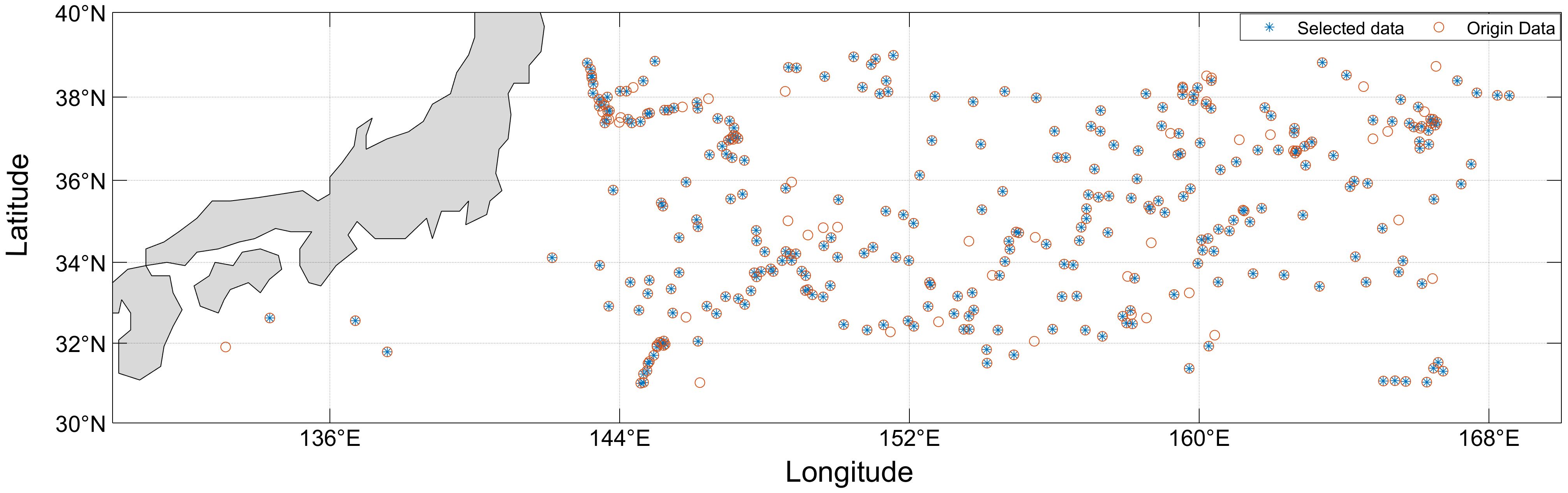
Figure 2 Distribution of Argo buoys after mass screening in the KE area (30°N-40°N, 130°E-170°E) in 2010.

2.1.4 Terrain data

This paper utilizes the ETOPO (ETOPO Global Relief Model) seafloor topography data provided by NCEI (National Centers for Environmental Information). This data set references a multitude of relevant models and regional measurements, incorporating global land topography and ocean bathymetry. Initially at a resolution of 1 arc-minute, it is interpolated to match the 1/12° grid resolution of the JCOPE2M data for the CZ test described in this paper (Amante and Eakins, 2009).

2.2 Methods

2.2.1 Mesoscale eddy identification methods

Given the extensive study area, we first divided it into the KE main body area (Area I) and the OC extension body area (Area II). Then, we applied the flow field geometry method and the closed curve method to identify sea surface temperature and salinity patterns, respectively.

The flow field geometry method is based on the geometric profile of the mesoscale eddies, which intuitively defines the mesoscale eddies as a region that meets certain constraints. If the velocity vector field in this region is a rotating flow, and the center of the mesoscale eddies are the extreme point of velocity, and the direction of the velocity vector around the point presents a symmetric structure, That is, the region is characterized by a clockwise or counterclockwise rotation of the velocity vector around a center, and such a structure is defined as an eddy structure.

The SLA closed curve method is directly based on detecting the closed curve of the sea surface height around a single local extreme value, with major advantages: they only use the SLA data, which significantly reduces the probability of non-closed eddies in the flow field geometry method. But the closed curve method also has its limitations: it needs to set the threshold of sea surface height difference to define the eddy boundary, which results in the subjective threshold will greatly affect the recognition result. In order to take into account the recognition effect of eddies and the sensitivity to the subjective threshold, we adopt a hybrid algorithm of the two.

The two identification methods above are used to identify the sea surface flow field and SLA data, respectively, to find the eddy pair with the largest intersection of the boundaries of the two methods at the same time (since the two methods have different parameter settings between different characteristic eddies, this paper defines a custom threshold: the intersecting area is greater than 50% of the respective area of each method, and the distance between the eddy centers is not more than 1/12°), and if the conditions are met then, the identification results of both methods are considered valid and the eddy is treated as an actual existing eddy with the eddy center identified by the flow field geometry method as the actual center. Figure 3 plots the identification of mesoscale eddies using the hybrid algorithm in the 30°N-40°N, 130°E-170°E region over the time span from January 1, 2007, to December 31, 2020. because of the large number of eddies, we represent the eddies as a single eddy center.

Figure 3

Figure 3 Schematic diagram of eddy identification (eddy centers) assembly in the region 30°N-40°N, 130°E-170°E from January 1, 2007, to December 31, 2020. (The orange point is the center position of the AE identification result for the time period, while the blue point is the CE).

Finally, in order to verify the reliability of the hybrid recognition algorithm, we use the algorithm and the two original algorithms to identify the results on a random day each year between 2007 and 2020, taking the hit rate of manually identifying the vortex center position falling within the vortex edge obtained by the three algorithms as an indicator, and repeating the 10-group averaging to obtain the overall recognition results. The correct matching rate of the hybrid algorithm is 91.5%, the closed contour method is 89.1%, and the flow field geometry method is 90.2%, proving that the hybrid algorithm is slightly better than the two original algorithms.

Additionally, we project the resulting eddy-identified location information onto the JCOPE2M grid point at the minimum distance from that grid point, thus enabling the connection between the two datasets.

2.2.2 Hydroacoustic calculation methods

In this paper, we first convert the JCOPE2M reanalysis temperature and salt data into sound speed data by utilizing the sound speed empirical formula. After statistical analysis, the temperature-salinity depth characteristics of the KE region are all consistent with the set threshold of the Chen-Millero sound speed empirical formula, so this paper adopts this formula to transform the temperature-salinity field data in the JCOPE2M data into the sound speed field data (Equation 1).

$$v=C_W(t,p)+A(t,p)S+B(t,p)S^{\raisebox{1ex}{$3$}\!\left/ \!\raisebox{-1ex}{$2$}\right.}+D(t,p)S^2$$

$$C_W(t,p)={\displaystyle \sum _{i=0}^5{C}_{0i}{t}^i}+{\displaystyle \sum _{j=0}^4{C}_{1j}{t}^{j}p}$$

$$A(t,p)={\displaystyle \sum _{i=0}^5{A}_{0i}{t}^i}+{\displaystyle \sum _{j=0}^4{A}_{1j}{t}^{j}p}+{\displaystyle \sum _{j=0}^3{A}_{2j}{t}^j{p}^2}+{\displaystyle \sum _{j=0}^2{A}_{3j}{t}^j{p}^3}$$

$$B(t,p)=B_{00}+B_{01}t+(B_{10}+B_{11}t)p$$

$\begin{array}{ll}D(t,p)=D_{00}+B_{01}p& (1)\end{array}$

where t is the temperature in °C, S is the salinity in ppt, $p$ is the pressure in bar. $A_{i,j},B_{i,j},C_{i,j},D_{i,j}$ is the setup parameter, please refer to the paper (Chen and Millero, 1977) for detailed values (Table 1). $Bellhop$ is a model based on a Gaussian beam-tracking algorithm to compute the sound field in a uniform or non-uniform environment (Porter and Bucker, 1987). The model associates each acoustic ray with a Gaussian intensity as the central acoustic ray of the Gaussian beam, and the propagation process of the simulated acoustic ray is more consistent with the results of the full-wave model and has been widely used in the field of acoustic computation (Gul et al., 2017). The evolution of the sound beam in this model is determined by the beam width $p(s)$ and the beam curvature $q(s)$, with $p$ and $q$ being controlled by the following differential equations (Equations 2–7):

$\begin{array}{ll}\begin{array}{l}\frac{dq}{ds}=c(s)p(s)\\ \frac{dp}{ds}=\frac{c_m}{c^2(s)}q(s)\end{array}& (2)\end{array}$

Table 1

Table 1 Scope of application of the Chen-Millero sound speed empirical formula.

where $c_m$ is the speed of sound and $c(r,s)$ is the second derivative with respect to the path direction, as shown in the following equation:

$\begin{array}{ll}{c}_m=c_{rr}{\left(\frac{dr}{dn}\right)}^2+2c_{rz}\left(\frac{dr}{dn}\right)\left(\frac{dz}{dn}\right)+c_{zz}{\left(\frac{dz}{dn}\right)}^2& (3)\end{array}$

$\begin{array}{ll}{c}_m=c_{rr}{(N_{(r)})}^2+2c_{rz}(N_{(r)})(N_{(z)})+c_{zz}{(N_{(z)})}^2& (4)\end{array}$

where $(N_{(r)})(N_{(z)})$ is the unit normal in both directions and can satisfy:

$\begin{array}{ll}(N_{(r)})(N_{(z)})=\left(\frac{dz}{ds},-\frac{dr}{ds}\right)=c(s)[\zeta (s),-\rho (s)]& (5)\end{array}$

In summary, the beam can be defined as:

$\begin{array}{ll}u(s,n)=A\sqrt{\frac{c(s)}{rq(s)}}{e}^{(-iw\left\{\tau (s)+0.5[p(s)/q(s)]n^2\right\})}& (6)\end{array}$

where $A$ is a constant determined by the properties of the sound source; $n$ is the vertical distance from the acoustic ray to the sound source; $\omega$ is the angular frequency of the sound source. Finally, we apply weighting to the sound beam:

$\begin{array}{ll}A(s)=\delta \alpha \left(\frac{1}{c_0}\right)\sqrt{\frac{q(s)\omega \cos \alpha }{2\pi }}{e}^{(\frac{i\pi }{4})}& (7)\end{array}$

where $\delta \alpha$ is the angle between the beams. In this paper, the main parameters of the sedimentary layers in the study area when using the $Bellhop$ ray theory model are listed in Table 2, and we choose $Abyssal Clay$ as an example to be studied in this paper.

Table 2

Table 2 Acoustic parameters of the three main types of sedimentary layers in the study area.

The CZ is a concentrated area of strong acoustic energy that occurs when a sound source is in the surface and subsurface layers of the ocean and, due to the refraction and propagation of sound waves over a wide range of areas, converges again near the sea surface several tens of kilometers away. Typical changes in the marine environment can cause changes in the structure of the sound velocity and thus have an impact on sound propagation in the CZ. Based on synthetic eddy data and $Bellhop$ model, the Marine environment with warm eddy, cold eddy and no eddy is analyzed respectively. The acoustic propagation was simulated, and the acoustic propagation loss field of 0m-1,000m was obtained, as shown in the figure, which was obvious on the offshore surface. The CZ is the area where the sound propagation loss is small (Figure 4).

Figure 4

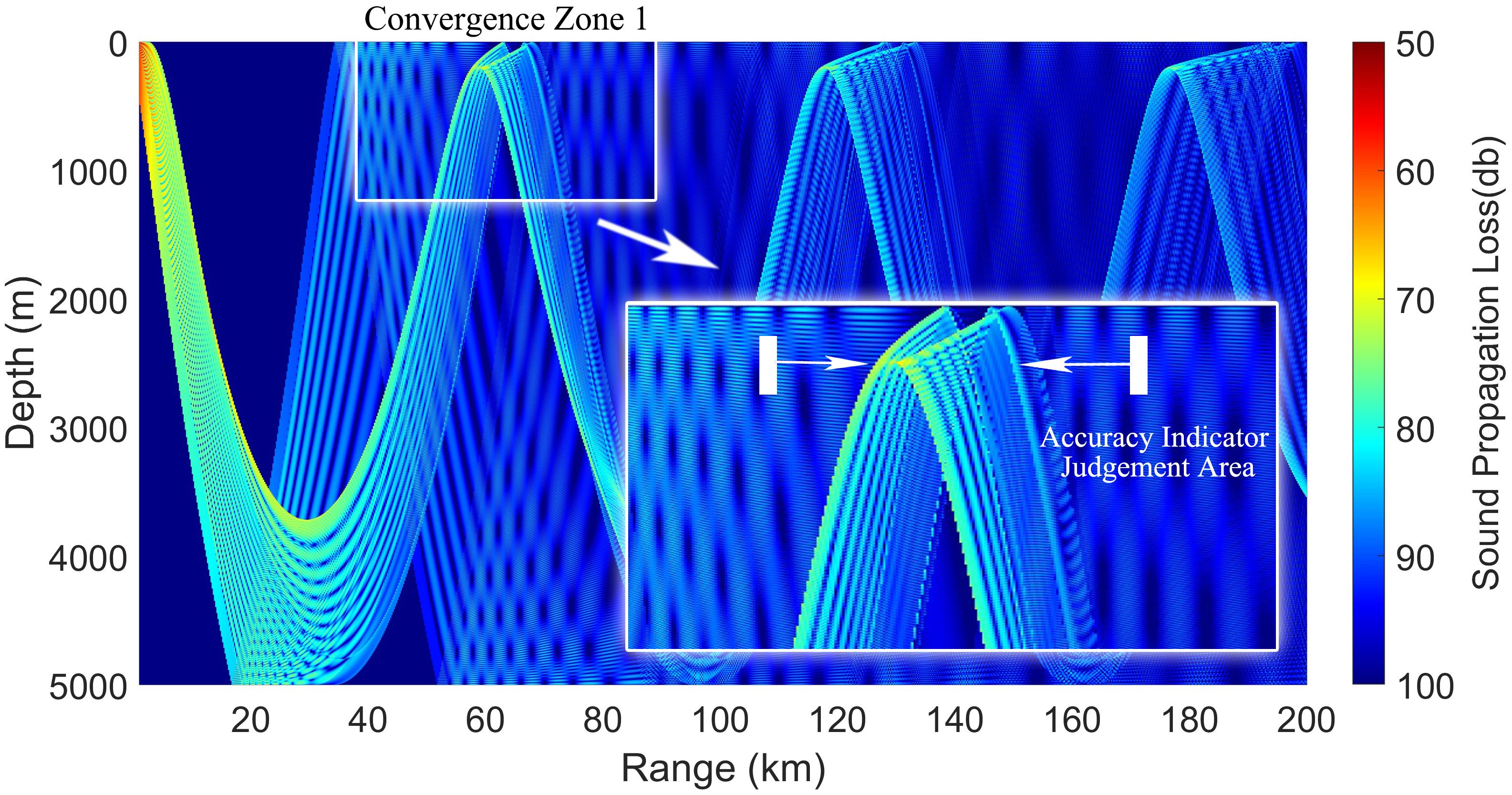
Figure 4 Schematic representation of acoustic propagation loss and CZ assessment metrics for the Bellhop model applied to the Munk example sound speed profile.

2.2.3 Sample set of mesoscale eddy sound speed profile

Using the eddy center and profile information obtained from the mesoscale eddy mixing identification algorithm, we differentiate between cold and warm eddies. To generate the SSP dataset, we employ a method that creates multi-angle vertical sections through the eddy center. Specifically, in order to avoid confusing other eddy structures during the extraction of individual profiles, it has been concluded through extensive experiments that lines are drawn along both sides at a distance of 1.2 times the eddy radius in the longitudinal and latitudinal directions, respectively, and the profiles are extracted vertically downwards, as shown schematically in the black rectangular box in Figure 5. Along this line, we create vertical SSPs from 0 to 1000m (Sandalyuk et al., 2020). Repeating the process at 30° intervals (or less) which is depending on how many SSP samples the researchers want to extract from a single eddy. A closed contour screening method is used to exclude poor data. From this method, we have obtained a total of 51,552 SSPs for warm eddies and 37,801 for CEs. Additionally, we use the two-dimensional deep-ocean Gaussian eddy model to produce a dataset comprising 20% of these profiles.

Figure 5

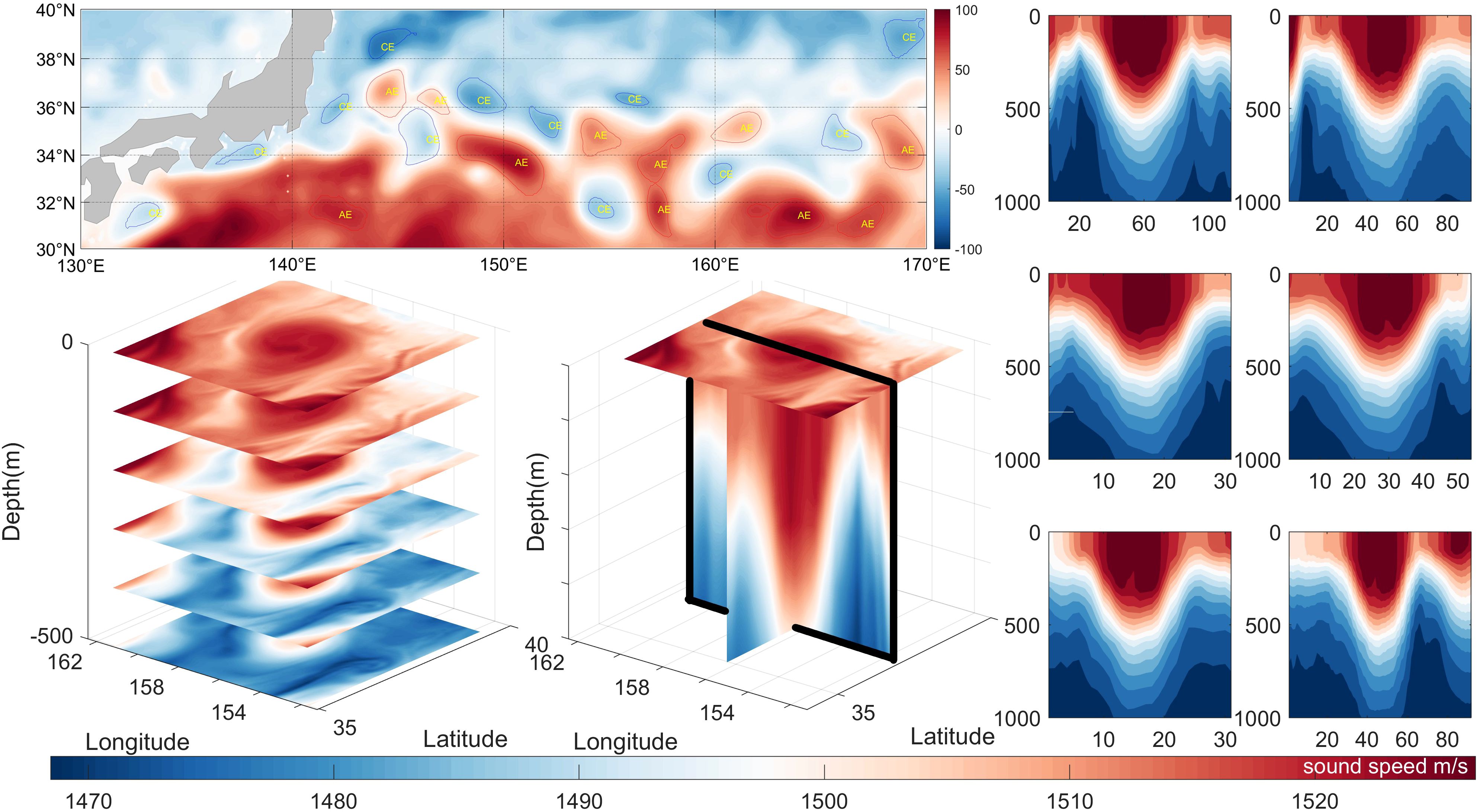
Figure 5 Schematic illustration of the extraction method and effect of mesoscale eddy sound speed profile dataset (The top left shows the results of the mesoscale eddy identification, and the right image shows the SSP extraction results for the example).

3 Modeling and evaluation criteria

3.1 Two-dimensional slow-variable deep-sea Gaussian eddy modeling

The mesoscale eddy ideal model is constructed based on the feature information extracted from sea surface observations, and the sound speed expression of the model is (Equations 8–10):

$\begin{array}{ll}c(r,z)=c_0(z)+\delta c(r,z)& (8)\end{array}$

$\begin{array}{ll}{c}_0(z)=C_1\left\{1+0.00741[e^{-\eta }-(1-\eta )]\right\}& (9)\end{array}$

$\begin{array}{ll}\delta c(r,z)=DC\times e^{-(\frac{r-Re}{D{R}^2\frac{z-Ze}{D{Z}^2}})}& (10)\end{array}$

Where $r$ is the horizontal distance to the eddy center, and $z$ is the vertical distance to the eddy center. For the Munk profile model (Munk, 1950), $\eta =2(z-z_1)/1300$​, is the sound speed at the sound channel axis and ​ is the depth at the sound channel axis. $DC$ is the eddy strength, which takes a negative value for CEs and a positive value for AEs. $DR$ is the horizontal radius of the eddy, $DZ$ is the vertical radius of the eddy, $Re$ is the horizontal position of the eddy center, and $Ze$ is the vertical position of the eddy center. The eddy strength is calculated from the sea surface height anomaly, and the horizontal radius of the eddy is determined as 1.2 times the maximum radius of a single eddy in the eddy identification results in section 2.2.1, and the vertical radius of the eddy and the vertical position of the eddy center are calculated from the eddy-centered Argo data captured by a single eddy. The Gaussian eddy model is schematically shown in Figure 6.

Figure 6

Figure 6 Schematic of a two-dimensional slow-varying Gaussian eddy model. In the case of the AE, for example, the parameters are set to $AE:DC=50cm,DR=20km,DZ=300m ;CE:DC=-30cm,DR=20km,DZ=300m$.

3.2 Advanced generative adversarial network model (EddyGAN)

The fundamental concept of the native GAN (Goodfellow et al., 2014) is to engage two neural networks in a continuous minimax game, where the networks learn the distribution of actual samples over time. The training is typically deemed complete when both networks reach a Nash Equilibrium.

In Figure 7, the generator network (denoted as $G$) receives a random variable (denoted as $z$) from the hidden space (denoted as $p_z$) as input, and the output is a generated sample. The goal of training the generator is to enhance the similarity between the generated sample and the real sample to the point where the discriminator (denoted as $D$) network cannot differentiate between them. This aims to make the distribution of the generated sample (denoted as $p_g$) as close as possible to the distribution of the real sample (denoted as $p_{data}$). The discriminator’s input is either real samples (denoted as $x$) or generated samples (denoted as $x\text{'}$), with the output being the discrimination result. The discriminator’s training objective is to accurately distinguish real samples from generated samples. This result is used to calculate the loss function and update the network weights through backpropagation. During adversarial training, the discriminator’s ability to identify real versus fake samples improves, while the generator strives to produce samples that are increasingly indistinguishable from actual samples, thereby deceiving the discriminator. Ultimately, the model generates higher-quality new data. The training objective of the native GAN network can be summarized as follows: to minimize the distance between $x$ and $x^{\prime }$ and to maximize the accuracy rate of the discriminator’s sample classification, where the value for real samples tends to be 1 and for fake samples tends to be 0. From this, we derive the native GAN network objective function (Equation 11).

Figure 7

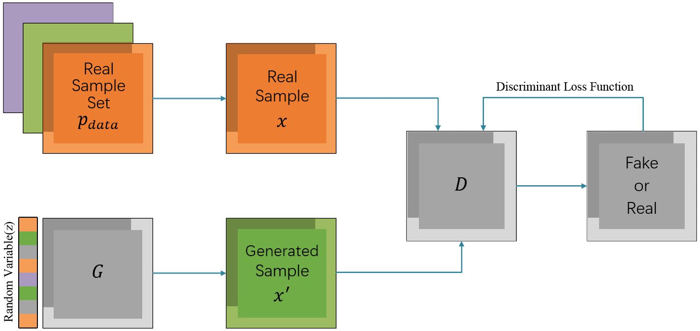
Figure 7 Schematic of the basic model of a native GAN network.

$\begin{array}{ll}\frac{min}{G}\frac{max}{D}{E}_{x~p_{data(x)}}[logD(x)]+E_{z~p_{z(x)}}[log(1-D(G(z)))]& (11)\end{array}$

Building on the native GAN, this paper introduces a generative adversarial network model adapted for mesoscale eddy reconstruction applications named EddyGAN. This model is inspired by the concept of global and local context codecs from Iizuka et al (Iizuka et al., 2017), featuring a generator and two context discriminators.

3.2.1 Generator

In order to improve the generation efficiency of the generator and make the adversarial network converge quickly, we utilize the Two-dimensional slow-variable deep-sea Gaussian eddy modeling in 3.1 as a priori knowledge to replace the Gaussian noise in the generator, and this achieves a better-expected result in the experiments. The EddyGAN generator relies on a fully convolutional network aimed at completing missing data. To enhance the training effectiveness, we utilize several convolutional layers with different strides alongside dilation convolutional layers of matching strides (Yu et al., 2017). After each convolutional layer, a Rectified Linear Unit (ReLU) is added, and the output layer is followed by a Sigmoid activation function to normalize the output. The architecture of the generator network is depicted in Figure 8.

Figure 8

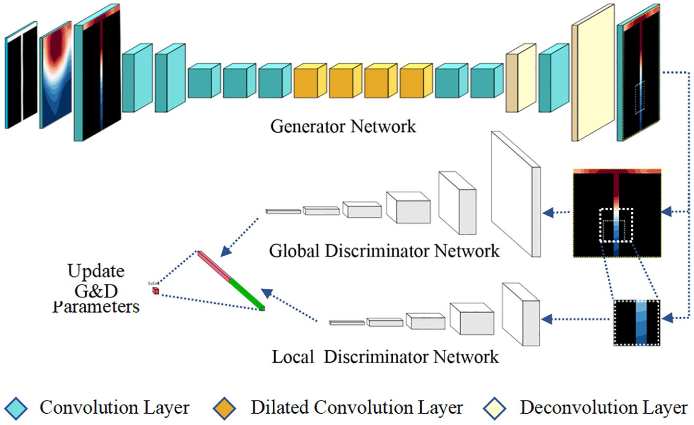
Figure 8 Schematic model of EddyGAN network.

In order to construct the reconstruction environment under data-poor, we simulate the reconstruction conditions with only the sea surface sound velocity field and Argo sound velocity contour by using a large-area mask to mask the data that are not in these two regions (i.e., assigning 0), and setting the width of the sea surface data and the Argo data to 1. The generator will not generate the data of the unmasked region when it is working, and will instead generate the data of the masked region, so as to achieve the goal of not varying the known portion of the data and to be able to generate the new data. We initially reduced the computational load by lowering the data resolution before training. Afterward, an inverse convolutional network is used after the output layer to restore the image to its original resolution.

Equation 12 details the convolution operation of the dilated convolutional layer for each pixel. The introduction of the dilated convolutional layer serves to expand the receptive field without increasing the parameter count, which experimentally has been shown to enhance the network’s perception of the eddy’s overall features, whether local or global. Here, $k_w$ and $k_h$ represent the width and height of the convolution kernel, $\eta$ is the dilation parameter, $x_{u,v}\in {ℝ}^C$ and $y_{u,v}\in {ℝ}^C$ are the input and output pixels of the layer, respectively, $\sigma$ is a nonlinear transfer function, $W_{s,t}$ is the convolution kernel matrix, $b\in {ℝ}^{C }$ is the bias vector for the convolutional layer, and when $\eta =1$, Equation 12 reverts to the standard convolution operation.

$\begin{array}{ll}\begin{array}{c}{y}_{u,v}=\sigma \left(b+{\displaystyle \sum _{i=-k_h^{\text{'}}}^{k_h^{\text{'}}}{\displaystyle \sum _{j=-k_w^{\text{'}}}^{k_w^{\text{'}}}{W}_{k_h^{\text{'}}+i , k_w^{\text{'}}+j}{X}_{u+\eta i ,v+\eta j}}}\right) , k_h^{\text{'}}\\ =\frac{k_h-1}{2} , k_w^{\text{'}}=\frac{k_w-1}{2}\end{array}& (12)\end{array}$

The network is trained with input-output pairs to minimize the loss function between them.

3.2.2 Discriminator

We train one global context discriminator and one local context discriminator to discern whether the output is real. The purpose of constructing a global context discriminator is to reconstruct the characteristics of the eddy as a whole, emphasizing to guide the model to pay more attention to the relationship between sea surface data and Argo data, while the local context discriminator pays more attention to local details. Especially for the training of eddy core position, due to the different characteristics of different vortices, we set the local context discriminator window within the range of 400-700 meters, that is, the window is not fixed. The global context discriminator consists of 5 consecutive convolutional layers, each with a stride of 2. It processes the input data of size 256×256 into a single 1024-dimensional vector using a fully connected layer followed by a sigmoid output layer. The local context discriminator, comprising 6 consecutive convolutional layers also with a stride of 2, focuses on a 128×128 patch at the center of the completed region. It outputs a 1024-dimensional vector that reflects the local context effects within that region. The outputs of the global and local discriminators are concatenated to form a single 2048-dimensional vector, which is then transformed into a continuous and normalized probability distribution of being real via a fully connected layer and a sigmoid transfer function.

3.2.3 Training

To address the issues of training stability and acoustic field reconstruction accuracy in GAN networks, we employ a combined loss consisting of Mean Squared Error (MSE) and GAN loss (Goodfellow et al., 2014), a method proven effective in experiments by Pathak et al (Pathak et al., 2016). Thus, following the max-min principle of GAN networks, we define the objective function (Equation 13): where $M_d$ and $M_c$ are stochastic masks used to simulate eddy acoustic field preconditioning, and $\alpha$ represents weighted hyperparameters.

$\begin{array}{ll}\begin{array}{l}\frac{min}{G}\frac{max}{D}\mathbb{E} [ L(x,M_c)+logD(x,M_d)+\alpha \text{log}(1-D(G(x,M_d),M_c) ]\\ L(x,M_c)={\Vert M_G\odot (G(x,M_c)-x)\Vert }^2\end{array}& (13)\end{array}$

The training process is divided into three phases: initially, the generator network is trained iteratively A times using MSE loss alone. After this phase, training of the generator is halted, and the discriminator network is trained independently $B$ times. Finally, the generator and the context discriminator networks are trained synchronously $C$ times. To prevent instability during training, we balance the gradient of MSE loss for the generator network with the gradient for the discriminator network (Equation 14) while applying standard gradient descent.

$\begin{array}{ll}\begin{array}{l}\mathbb{E} [\text{ ∇ }L(x,M_c)+\alpha \nabla log(1-D(C(x,M_c)),M_c)]\\ \mathbb{E} [\nabla logD(x,M_d)]\end{array}& (14)\end{array}$

In network optimization, we utilize the Adam optimization algorithm (Kingma and Adam, 2015). The hyperparameters of the Adam optimizer are intuitive and often require minimal or no fine-tuning. This optimizer is generally considered to perform well by default, as verified by numerous experiments conducted by scholars (Zhang, 2018). Regarding the setting of the hyperparameters of Adam optimizer, in general, the learning rate is set between 0.0001~0.1, too high will make the model training effect poor, too low will make the model training converge slowly, so through many adjustments, we determine the learning rate is 0.0002, corresponding to the appropriate increase in epoch to 400000. ${\beta }_1$ and ${\beta }_2$ are important hyperparameters in Adam optimizer, usually taking values of 0.9 and 0.999. If the dataset is noisy, try to reduce ${\beta }_1$ and ${\beta }_2$, even though the average coefficients converge faster but are more susceptible to noise. If the dataset is less noisy, ${\beta }_1$ and ${\beta }_2$ can be increased to update the parameters more consistently. In this paper, ${\beta }_1$ = 0.9 and ${\beta }_2$ = 0.999 are set.

3.3 Training assessment indicators

In this paper, two metrics, Root Mean Square Error (RMSE) and Structural Similarity Index (SSIM) (Wang et al., 2004), are used for evaluating mesoscale eddy reconstruction, with the forecast accuracy of the CZ serving as an auxiliary metric. For the effect of mesoscale eddy reconstruction, not only the overall error size should be considered, but also its structural characteristics should be taken into account, so we consider it in two aspects: numerical error index and structural similarity index. There are many numerical error indicators, after weighing, we choose the RMSE indicator in $L2$ paradigm, which is often used in 2D matrix error analysis. Compared with $L1$ paradigm indicator, $L2$ paradigm indicator is sensitive to the larger outliers in the error, which is better for the response to the anomalous noise that is likely to appear in the reconstruction results, and is more helpful for comparing the reconstruction effect. For the structural similarity index, we choose the SSIM index, which has the widest application range and the highest validity.

3.3.1 Root mean square error

RMSE is a common metric for assessing the discrepancy between model predictions and actual observations; generally, a lower value indicates a better outcome. The relevance of RMSE to data size and dimensionality necessitates uniform adjustment of two-dimensional SSP data in this paper to ensure the validity of inferences about the dimensionality of the SSP data. The two-dimensional (Equation 15) between predicted and target data are calculated as follows:

$\begin{array}{ll}\begin{array}{c}RMSE=\sqrt{\frac{1}{H\times W}{\displaystyle \sum _{i=1}^H{\displaystyle \sum _{j=1}^W{(X(i,j)-Y(i,j))}^2}}} i\\ =1,2,3\dots H ;j=1,2,3\dots W\end{array}& (15)\end{array}$

Equation 15 represents the two-dimensional RMSE calculation formula, where $H$ and $W$ denote the length and width of the data, respectively, and $X$ and $Y$ represent the predicted and original data. It is important to note that to mitigate the impact of large errors on the overall evaluation, this paper employs the 3-sigma rule to exclude outliers from the RMSE calculation (Equation 16), where $\sigma$ is the standard deviation, and $\mu$ is the mean value.

$\begin{array}{ll}P(\left|x-\mu \right|>3\sigma )\le 0.03& (16)\end{array}$

3.3.2 Structural similarity index

The SSIM is a measure of data’s structural similarity (Hore and Ziou, 2010). Given two data sets $x$ and $y$, their structural similarity is defined by Equations 17 and 18:

$\begin{array}{ll}SSIM(x,y)=\frac{(2{\mu }_x{\mu }_y+c_1)(2{\sigma }_{xy}+c_2)}{({\mu }_x^2+{\mu }_y^2+c_1)({\sigma }_x^2+{\sigma }_y^2+c_2)}& (17)\end{array}$

$\begin{array}{ll}{c}_1={(k_{1}L)}^2 , c_2={(k_{2}L)}^2 & (18)\end{array}$

Where ${\mu }_x$ is the mean value of $x$, ${\mu }_y$ is the mean value of $y$, ${\sigma }_x^2$ is the variance of $x$, ${\sigma }_x^2$ is the variance of $y$, and ${\sigma }_{xy}$ is the covariance of $x$ and $y$. $L$ is the dynamic range of the pixel value, which is set to 100, and $k_1 ,k_2$ are the constants, which $k_1,k_2$ are set to 0.01 and 0.03 in this paper.

3.3.3 Accuracy of CZ renconstruction

In this paper, we use acoustic convergence zone reconstruction accuracy for assisted evaluation. The definition of acoustic convergence zone is reflected in 2.2.2 of the paper, we will be the acoustic propagation loss minima on both sides of the range of 3km for the convergence zone hit zone, if the reconstructed acoustic convergence zone minima fall within the hit zone of the real acoustic convergence zone, it will be judged as a successful reconstruction in this way, and vice versa, it will be a failure. In this paper, we mainly focus on the first three acoustic convergence zones as the main research object.

4 Mesoscale eddy sound field reconstruction effect

4.1 Evaluation of the effect of numerical errors

In this paper, we first apply the EddyGAN model to reconstruct the acoustic field of a mesoscale eddy using JCOPE2M reanalysis data from the Kuroshio Extension (30°N-40°N, 130°E-170°E). The input conditions for the model include the sea surface sound velocity field of the complete eddy structure and one to five SSPs: the sea surface sound speed field is calculated from the sea surface temperature and salinity by the empirical formula for the sound speed, and the SSPs are obtained from measurements made by the Argo or other vertically suspended temperature and salinity depth measurement instruments (e.g. CTD, XBT, etc.) and calculated using the empirical formula for the sound velocity.

We artificially constrained the input conditions for the different cases:

(1) For the case of a single SSP with a sea surface sound velocity field input, we set the position of this SSP to be no more than 10% of the horizontal radius of the eddy body;

(2) For the case of two SSPs with sea surface sound velocity field inputs, we set the two SSPs to be located on either side of the eddy center;

(3) For the case of greater than three SSPs with sea surface sound velocity field inputs, we restricted them to only those whose positions do not overlap with respect to the eddy center.

As shown in Figure 9 and Figure 10, regarding eddy characteristics under single-profile conditions, the SSIM metric for AEs averages 0.70, ranging from 0.6 to 0.9, and the RMSE averages 1.4 m/s, with a distribution between 1.3 m/s and 1.5 m/s. In contrast, for CEs, the average SSIM metric is 0.61, with a range of 0.50 to 0.70, and the RMSE averages 2.0 m/s. These results indicate that EddyGAN’s reconstruction similarity or error index for AEs is significantly better than that for CEs. This may be attributed to two factors: the larger sample size of AEs compared to CEs, which allows for more extensive learning within the same epoch, and the better connectivity of warm eddies with the mixing layer at the sea surface. Meanwhile, CEs display a larger sound speed gradient near the sea surface, which is not captured during the swell convolution process in the model, resulting in the loss of some information and poorer reconstruction outcomes.

Figure 9

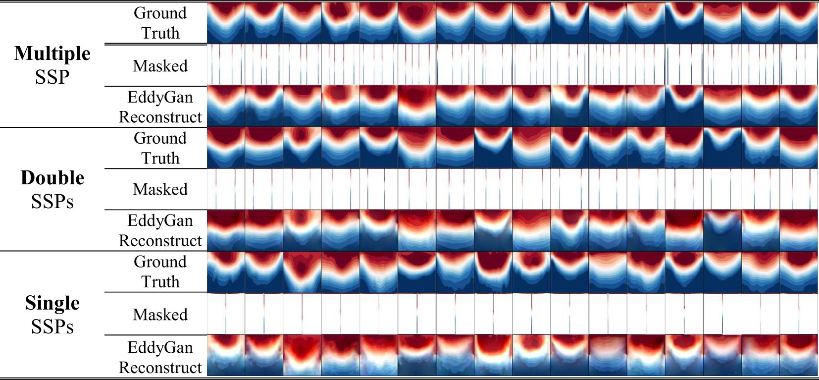
Figure 9 Schematic diagram of the effect of EddyGAN acoustic field reconstruction (as an example under One to Multiple SSPs of different quantities).

Figure 10

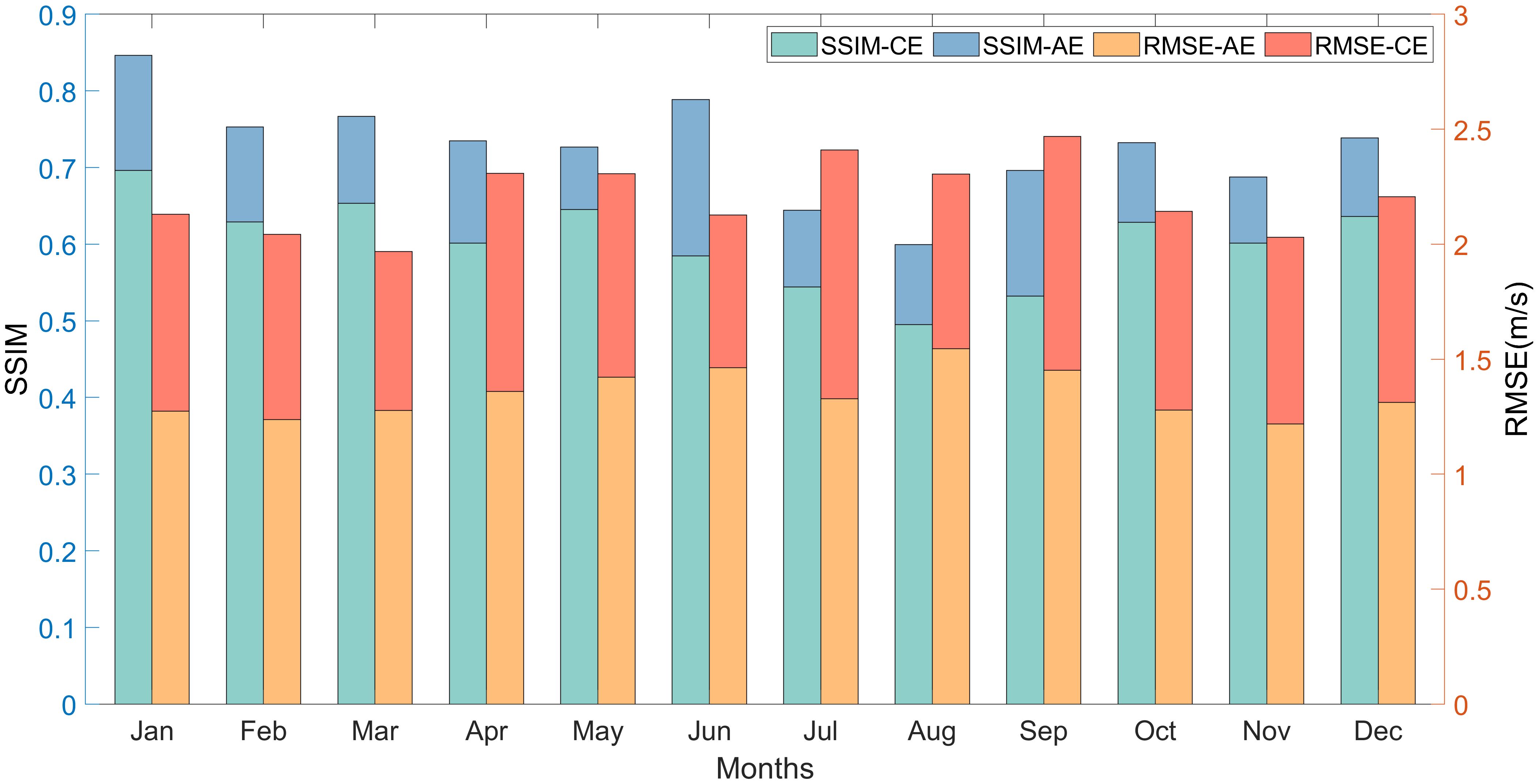
Figure 10 Schematic diagram of the effect of EddyGAN acoustic field reconstruction (as an example under a single SSP).

From the reconstruction results of each month, the SSIM index for June to September is notably lower than for other months, and the RMSE is slightly higher than the average. This suggests that the reconstruction quality during these months is inferior in terms of structural similarity and average error. Possible reasons for these findings include: firstly, June to September is the period of the highest direct solar intensity in the Northern Hemisphere, leading to a strong stirring of the sea surface mixed layer and less distinct features of sea surface temperature, salinity, and sound speed fields, therefore diminishing the model’s learning effectiveness; secondly, the average intensity and lifespan of eddies peak during these months (Hu et al., 2018), which often leads to the reduction in the number of valid samples in the sample set, and the reason for this is that because of the higher strengths and lifetimes of the vortices in these months, the methodology that we used to extract the samples does not constrain the process of repeated extractions of the same eddy, which results in the long-lived and strong eddies in the sample set being extracted in that time period. This leads to a relative reduction in the effective sample data since eddies with long lifetimes and high intensities are repeatedly extracted during the extraction of the sample set and have similar characteristics.

To investigate the impact of different numbers of SSPs on the reconstruction effect, we randomly selected 1000 SSPs and applied the EddyGAN model to reconstruct them. The results were assessed using the average SSIM and RMSE indices within the group. Considering practical application, the number of SSPs in the control experimental group for this paper is set at a maximum of 5. The maximum value of 5 SSPS is set because this paper mainly uses Argo buoy data for reconstruction in combining theory with practice. Combined with the pre-processing of Argo data in 2.1.3, we found that most (almost all) of the eddy-captured Argos that meet the reconstruction conditions (see Section 5.2) are less than 5. Therefore, considering the actual application scenario of the model in this paper, we only conducted experiments on SSPS within 5. As shown in Figure 11, the median SSIM and RMSE for AEs are maintained at approximately 0.72-0.85 and 1.0-1.5 m/s, respectively, while those for CEs range from 0.65-0.75 and 1.0-2.0 m/s. Overall, the SSIM and RMSE indices for AEs are significantly better than those for CEs, consistent with prior experimental outcomes. The reasons for this have been delineated in previous sections and will not be reiterated here. From the perspective of each control group, the median SSIM index shows a positive correlation with the number of SSPs for both warm eddies and CEs, whereas the median RMSE index exhibits a negative correlation. The first and third quartiles demonstrate similar trends to the median, suggesting that as the number of SSPs increases, the reconstruction effect of EddyGAN also improves, particularly from 1 to 3 SSPs. The improvement then decelerates and becomes more variable at 5 SSPs. This indicates that the reconstruction effect tends to stabilize when using 5 SSPs.

Figure 11

Figure 11 Boxplots of SSIM, RMSE metrics for EddyGAN acoustic field reconstruction with different numbers of SSP.

We also compare the SSIM and RMSE metrics of several commonly used reconstruction methods with the reanalyzed data, considering the distinction between AEs and CEs. The test data were grouped based on mesoscale eddy characteristics (AE, CE), and to avoid uncontrollable errors due to variance in the number of SSPs across different months during random sampling, the test samples for each group are equally drawn from different months and varying numbers of SSPs. The results are then averaged within each group and are presented in Table 3. To demonstrate the improvement of the reconstruction effect of the EddyGAN model by using deep-sea slowly changing Gaussian vortex prior, we conducted an additional set of controlled experiments, and the experimental results were also marked * in Table 3.

Table 3

Table 3 Indicators for evaluating the effectiveness of multiple mesoscale eddy acoustic field reconstruction methods.

From the table data, it is evident that the reconstruction effect of EddyGAN under different input conditions is significantly superior to that of several other traditional reconstruction methods. Both RMSE and SSIM indices achieve higher levels of improvement compared to the other methods. The SSIM indices, in particular, are also markedly higher, indicating that the data error with the EddyGAN method is considerably lower, and it more accurately describes the structural characteristics of the eddy acoustic field.

4.2 Convergence zone-based calibration assessment

Since the numerical error evaluation index in section 4.1 can mostly reflect the reconstructed data’s effect at an overall level, for specific acoustic effects such as the CZ that we are concerned with, it is necessary to use a theoretical model to perform secondary calculations based on the reconstructed acoustic field. Therefore, the purpose of this subsection is to provide an additional assessment of the EddyGAN reconstruction effect using the acoustic CZ reconstruction results (Xu et al., 2024).

The properties of the CZ play an important role in underwater applications. For example, in underwater communication and sonar detection, the properties of the CZ can be utilized to enhance the strength and clarity of signals and improve the efficiency and accuracy of communication and detection. In addition, the study of CZ also helps us to better understand and utilize the propagation law of underwater acoustics, which provides more reliable technical support for underwater operations, environmental monitoring, resource exploration and other fields. Therefore, based on the underwater application scenario of CZ, this paper proposes to use the CZ reconstruction effect to assist the evaluation of EddyGAN model. This subsection employs the $Bellhop$ ray theory model to reconstruct the CZ for the test sets in the four cardinal and intercardinal directions: East-West (E-W), North-South (N-S), Northeast-Southwest (NE-SW), and Northwest-Southeast (NW-SE). The experiments are designed to minimize the influence of seasonality and the number of different SSPs on the reconstruction results from subsection 4.1 and to emphasize the representativeness of the model’s forecasting ability. To achieve this, we created five control groups, each with 1000 samples extracted from different months and with varying numbers of SSPs. The calculation results were averaged within each group for presentation in Table 4.

Table 4

Table 4 Reconfiguration assessment metrics for the first three CZs in different directions.

In the table, the Accuracy index is the percentage of the number of reconstructed distance errors within 3km (Figure 5) of the CZ in the overall number of reconstructed profiles. The model parameters are set as shown in Table 2, with the seafloor topography updated to ETOPO data and the rest of the parameters set as default.

From the comparison results in Table 4, it is evident that the reconstruction accuracy of the CZ of the EddyGAN model under the specified conditions can generally be maintained above 70% in all four directions. Across different directions, the effect of CZ reconstruction remains consistently at the same level given identical conditions. Regarding the trend of change, there is a slight decrease in model reconstruction accuracy as the distance of the CZ increases. Concerning the nature of the eddy, the accuracy of the reconstruction for AEs is significantly greater than that for CEs. This may be attributed to a lower number of identifications in cyclonic eddy extractions and a smaller sample set size compared to that of AEs, resulting in a less effective learning outcome for the EddyGAN model. Consequently, the reconstruction of the sound speed field for AEs is notably superior to that of CEs. This disparity is also due to the CZ calculation being based on the reconstructed sound speed field, as reflected in the results presented in the aforementioned table.

5 Validation and generalization of the model

5.1 Validation in different study areas

Study Area II is characterized as the Oyashio Extender area where mesoscale eddies significantly influence the oceanographic characteristics of both regions, as indicated in references (Qiu, 2001; Sun et al., 2022). Area II exhibits different dynamics compared to the KE area (Area I). To investigate the generalization capability of the EddyGAN model across different marine environments, this subsection describes the reconstruction of the eddy acoustic field in Area II using the EddyGAN model. The model’s performance is evaluated using RMSE, SSIM, and CZ accuracy metrics. The sample randomization mechanism applied is the same as in Subsection 4.2, and the results are displayed in Table 5.

Table 5

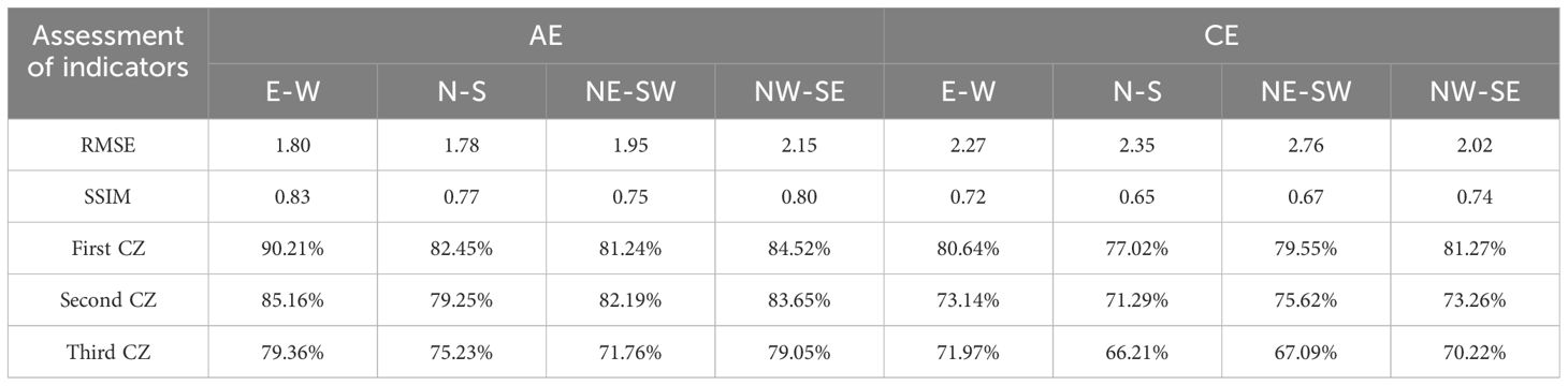
Table 5 Metrics for evaluating the effect of applying Eddy GAN model reconstruction in study area II.

The reconstruction index RMSE for Area II is maintained within the range of 1.80-2.76 m/s, and SSIM is within 0.65-0.83. The reconstruction accuracy for the first CZ lies between 77.02%-90.21%, for the second CZ between 71.29%-89.52%, and for the third CZ between 66.21%-79.36%. When compared to the overall reconstruction effect in Area I, as discussed in Chapter 4, it is apparent that Area II exhibits a slightly inferior performance in many aspects. This discrepancy can be attributed to the dataset construction, which utilized data from Area I, and the differences in geographic location, watershed characteristics, and eddy formation mechanisms between the two areas. Hence, the model tends to be more attuned to Area I rather than Area II. In terms of the CZ reconstruction, similar to the findings in 4.2, the accuracy diminishes as the distance of the CZ increases, indicating that more remote CZs pose greater challenges for model reconstruction.

5.2 Validation of the effect of eddy sound field reconstruction based on measured data

To further validate the generalizability of the EddyGAN model, we employ mesoscale eddy profiles constructed by fusing multiple Argo data from the WOA18 dataset for model validation.

Initially, we use the eddy identification information to match with the latitude and longitude of Argo data post-quality control screening. We extract data pairs with at least five Argos within 1.2 times the eddy radius. These pairs are relatively uniformly distributed across the eddy center and its peripheries, with pointwise first-order fitted straight lines passing through the eddy center’s extreme region. This matching data encompasses both Areas I and II. Subsequently, we applied the Akima interpolation method (Akima, 1970) to transform the discrete Argo profile data into continuous profiles. This interpolation method is also used to complement the WOA18 dataset’s temperature and salinity structures up to a depth of 1000 meters, necessary for subsequent CZ calculations. Finally, we calculate the sound speed data using the formula provided in Section 2.2.2. Using the aforementioned approach, we obtain the target set of measured eddy SSP, which are then reconstructed using the EddyGAN model, employing the same sampling mechanism as described in Subsection 4.2.

For the evaluation of effects, SSIM, RMSE, and CZ accuracy metrics are again utilized for assessment and comparison with the metrics from Regions I and II. The indicators for the first two regions are average values accounting for the number, direction, and month of SSP after sample re-randomization. The evaluation results are depicted in Figure 12.

Figure 12

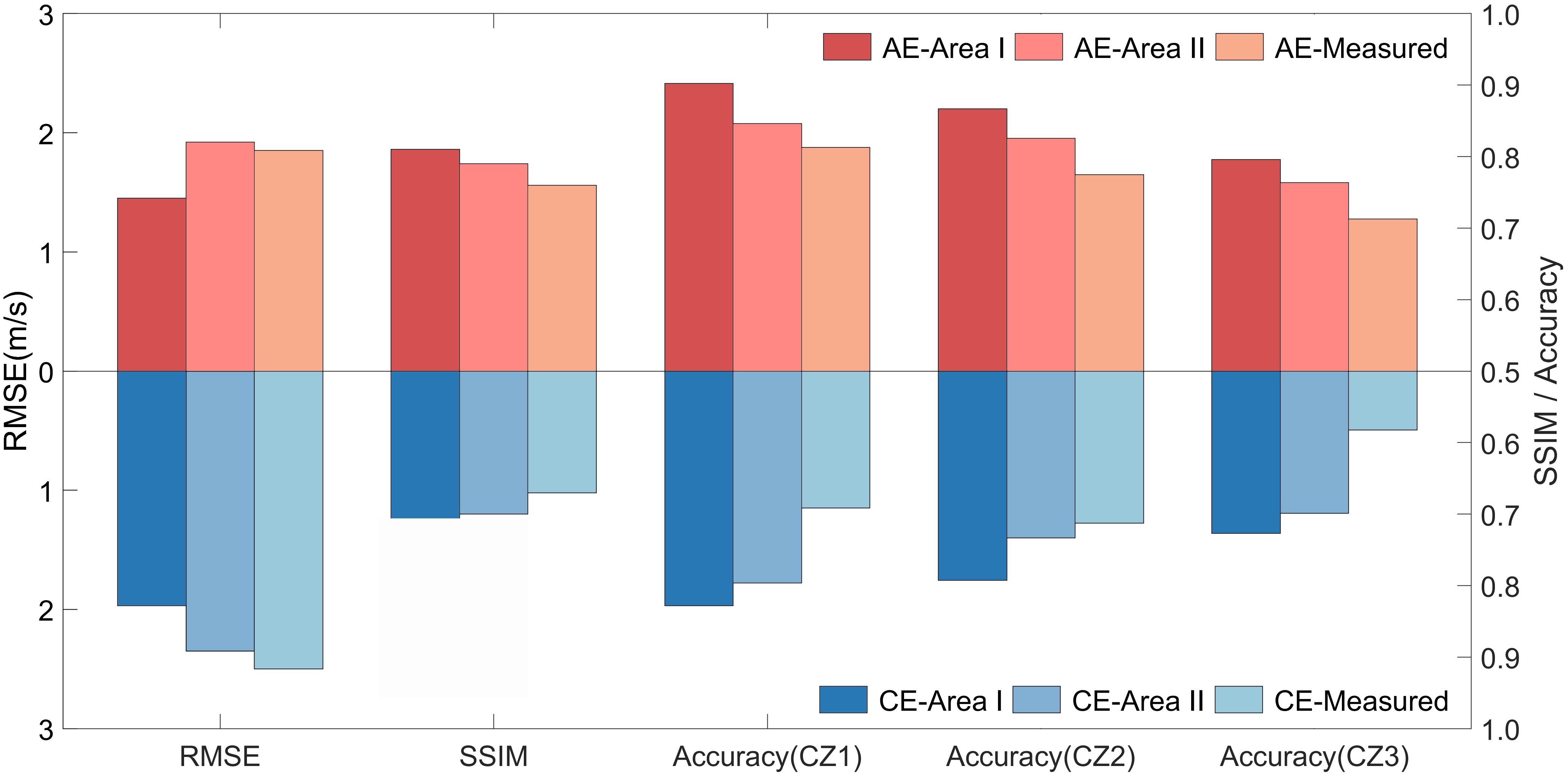
Figure 12 Schematic comparison of the indicators after applying EddyGAN reconstruction to the measured data of Area I and II.

In the case of warm eddies, the model exhibits greater effectiveness in reconstructing the sampling area (Area I), with an average SSIM of approximately 0.80, an average RMSE of around 1.50 m/s, and reconstruction accuracies exceeding 80% in the three CZs. In contrast, the reconstruction for Area II is marginally inferior; nevertheless, it still achieves an average SSIM of about 0.7, an RMSE of 2.0 m/s, and reconstruction accuracies surpassing 70% in the CZs. The average SSIM for Measured data stands at approximately 0.65. Regarding cold eddies (CEs), all indicators underperform relative to warm eddies (AEs), and this trend is consistent in the actual data reconstruction. As with AEs, the reconstruction effect in Area II is slightly less favorable compared to Area I, but with an average SSIM of around 0.7, an RMSE of about 2.0 m/s, and each CZ’s reconstruction accuracy exceeding 70%. The average SSIM for Measured data is approximately 0.65; with CEs, all indices are lower than those of AEs, which is also evident in the reconstruction of the Measured data (Figure 13).

Figure 13

Figure 13 Schematic comparison of the generalizability of the model for different input sound speed profile conditions, including Area 1, Area 2 and Measured Data (in the case of AEs).

From this analysis, we can deduce that the reconstruction effects in Areas I and II are in basic agreement with the experimental results presented in the previous paper. It is observed that the reconstruction quality of measured data is slightly inferior to that of reanalyzed data, and the reconstruction effect across different CZ distances exhibits a consistent trend with the reanalyzed data. Several factors may account for this: firstly, the sample size of the measured data is significantly smaller than that of the reanalysis data, which fails to capture the randomness ideally present; secondly, the model demonstrates better applicability to data that originates from the same source as the sample set, leading to somewhat weaker support for the measured data. Even though the reanalyzed data assimilate a considerable quantity of measurements from diverse sources, the volume of data is relatively limited for the expansive oceanic area. This limitation contributes to the measured data’s slightly less accurate reconstruction effect compared to the reanalyzed data. Despite the reanalyzed data incorporating extensive multi-source real measurements, the amount remains insufficient for the vast oceanic expanse, resulting in the model not fully capturing the characteristics of actual data. Thirdly, the measured data derived from the combination of WOA18 and Argo data, as introduced in this section, is not truly raw measured data. In comparison to shipborne survey measurements, there is a notable disparity in point density and instrumental precision. Consequently, this difference may also contribute to the challenge of accounting for the bias observed in the reconstruction effect.

Additionally, we have also carried out reconstructions of other high mesoscale eddy regions in the world’s oceans in our experiments, but the results were not good enough to be presented in the paper in the form of data visualizations. The reason is not difficult to explain, it is due to the dataset used in this paper is the Northwest Pacific region, so the model reconstruction effect for this region is much better than other regions, while the support for other regions needs to build additional sample datasets for training, which will be one of the directions of our future work.

6 Conclusion and outlook

In this paper, we utilized high-resolution reanalysis data and the mesoscale eddy identification technique based on flow field geometry to correlate eddy field information with corresponding mesoscale eddy temperature and salinity profiles. We adopted the empirical sound speed formula to create a sample dataset of mesoscale eddy SSPs. Subsequently, we proposed and trained a generative adversarial network model for mesoscale eddy reconstruction. The model was evaluated using SSIM, RMSE, and CZ reconstruction accuracy as indicators to assess its reconstruction performance. The results indicate that the model provides a better reconstruction effect. Compared with the native GAN network and traditional reconstruction methods, under the same sample set and parameter settings, the proposed Eddy GAN model displayed improvement. The average SSIM indices for AE and CE exceeded 0.75 and 0.65, respectively; the RMSE indices were 1.45 m/s for AE and 1.97 m/s for CE; and the reconstruction accuracy for CZ was above 70%, which is slightly higher than that of the native GAN network and significantly exceeds other methods.

During the experimental process, we observed four phenomena: first, the reconstruction effect for AE was significantly better than for CE; second, the reconstruction effect showed little variation across different directions; third, the reconstruction effect was poorer around the summer months in the northern hemisphere compared to other times of the year; and fourth, the reconstruction accuracy decreased with increasing distance of the CZ.

To verify the model’s generalizability and practical value, we used mesoscale eddy SSPs constructed by fusing multiple Argo datasets from WOA18 for model validation. We employed the same validation method to evaluate the model’s performance. The results demonstrate that the EddyGAN model performs well with real data, and the SSIM and RMSE metrics indicate performance comparable to the reanalyzed data. In terms of CZ accuracy, the reconstruction accuracy for the first two CZs was above 70%, while the third was slightly lower at 58%. Analyzing its causes, the poorer reconstruction results of the third CZ may be caused by the accumulation of its acoustic propagation error, which can be clearly seen in the decreasing reconstruction accuracy trend of the first, second, and third CZs in Figure 12. In addition, since the Measured data in this paper are synthesized from multiple Argo data that are approximately in a straight line, there is some synthesis error in itself, and the reconstruction accuracy of the CZ is closely related to the reconstruction effect of the profiles, so uncontrollable errors may occur; finally, since there are only about 200 sets of Measured data that meet the screening conditions in 5.2, the small amount of data may not be able to reflect the reconstruction effect more realistically. For the above reasons that may lead to the decrease of reconstruction effect, we give several possible solutions, which will also continue to be tried in our next research: first, updating the model to make it more applicable to the direction of mesoscale eddy reconstruction; second, expanding the sample dataset, which will lead to an increase in the content of the learning, and the model will be more generalizable and robust; third, fusing some of the measured data into the sample dataset instead of only using the reanalysis data to enhance its reconstruction support for the real data; fourth, the diversity of evaluation indexes; CZ reconstruction accuracy is admittedly a better application index to reflect the reconstruction effect, but other application evaluation indexes are more meaningful for the areas where CZs are less applied.

Finally, to address the challenge of reconstructing the mesoscale eddy sound field with limited data, we present the EddyGAN model as a solution. This model requires a minimum amount of data, specifically the sea surface sound speed field and a single sound speed profile at the eddy center. The model has undergone experimental evaluations to support its generalizability and validity, showing a degree of representativeness. However, there remains a gap in its response to the finer and more realistic mesoscale eddy sound field structures: limited by the collection range of the sample dataset, our proposed model is only applicable to the KE region and its adjacent regions with similar mesoscale eddy characteristics, while it is not as descriptive for other regions. In future work, we will build more models for sea areas with different mesoscale eddy characteristics to make our model more generalized and adapt it to the mesoscale eddy reconstruction conditions in more sea areas. If this research could incorporate a substantial number of mesoscale eddy survey data, the model’s credibility would significantly improve. We hope that this work will encourage the broader sharing of marine survey data and foster continued advancements in mesoscale eddy reconstruction research.

Data availability statement

The original contributions presented in the study are included in the article/supplementary material. Further inquiries can be directed to the corresponding author.

Author contributions

XM: Conceptualization, Investigation, Methodology, Software, Supervision, Writing – original draft, Writing – review & editing. LZ: Funding acquisition, Resources, Visualization, Writing – review & editing. WX: Formal analysis, Project administration, Validation, Writing – review & editing. ML: Data curation, Methodology, Supervision, Writing – review & editing. XZ: Data curation, Writing – review & editing.

Funding

The author(s) declare that no financial support was received for the research, authorship, and/or publication of this article.

Acknowledgments

Thanks to JAMEST for JCOPE2M data support (https://www.Jamstec.go.jp/jcope/htdocs/distribution/index.html). Thanks to NCEI for the bathymetric data ETOPO (https://www.ncei.noaa.gov/products/etopo-global-relief-model). Thanks to the AVISO for the mesoscale eddy dataset (https://www.aviso.altimetry.fr/en/data/products/value-added-products/global-mesoscale-eddy-trajectory-product.html). Thanks to the International ArgoProgram for providing the buoy dataset (https://argo.ucsd.edu/). Thanks to WOA18 for the climate state dataset support (https://www.ncei.noaa.gov/data/oceans/woa/WOA18/DATA/). Other scholars and organizations that helped in the research process are also acknowledged.

Conflict of interest

The authors declare that the research was conducted in the absence of any commercial or financial relationships that could be construed as a potential conflict of interest.

Publisher’s note

All claims expressed in this article are solely those of the authors and do not necessarily represent those of their affiliated organizations, or those of the publisher, the editors and the reviewers. Any product that may be evaluated in this article, or claim that may be made by its manufacturer, is not guaranteed or endorsed by the publisher.

References

Akima H. (1970). A new method of interpolation and smooth curve fitting based on local procedures. J. ACM (JACM) 17, 589–602. doi: 10.1145/321607.321609

CrossRef Full Text | Google Scholar

Akulichev V., Bugaeva L. K., Morgunov Y. N., Solovjev A. A. (2012). Influence of mesoscale eddies and frontal zones on sound propagation at the Northwest Pacific Ocean. J. Acoustical Soc. America 131, 3354–3354. doi: 10.1121/1.4708575

CrossRef Full Text | Google Scholar

Amante C., Eakins B. W. (2009). ETOPO1 arc-minute global relief model: procedures, data sources and analysis.

Google Scholar

Ashkezari M. D., Hill C. N., Follett C. N., Forget G., Follows M. J. (2016). Oceanic eddy detection and lifetime forecast using machine learning methods. Geophysical Res. Lett. 43, 12,234–12,241. doi: 10.1002/2016GL071269

CrossRef Full Text | Google Scholar

Chaigneau A., Le Texier M., Eldin G., Grados C., Pizarro O. (2011). Vertical structure of mesoscale eddies in the eastern South Pacific Ocean: A composite analysis from altimetry and Argo profiling floats. J. Geophys. Res.: Oceans 116. doi: 10.1029/2011JC007134

CrossRef Full Text | Google Scholar

Chelton D., Schlax M. G., Samelson R. M. (2011). Global observations of nonlinear mesoscale eddies. Prog. Oceanography 91, 167–216. doi: 10.1016/j.pocean.2011.01.002

CrossRef Full Text | Google Scholar

Chen C. T., Millero F. J. (1977). Speed of sound in seawater at high pressures. J. Acoustical Soc. America 62, 1129–1135. doi: 10.1121/1.381646

CrossRef Full Text | Google Scholar

Dong C., McWilliams J. C., Liu Y., Chen D. (2014). Global heat and salt transports by eddy movement. Nat. Commun. 5. doi: 10.1038/ncomms4294

CrossRef Full Text | Google Scholar

Duo Z., Wang W., Wang H. (2019). Oceanic mesoscale eddy detection method based on deep learning. Remote Sens. 11, 1921. doi: 10.3390/rs11161921

CrossRef Full Text | Google Scholar

Endoh T., Hibiya T. (2001). Numerical simulation of the transient response of the Kuroshio leading to the large meander formation south of Japan. J. Geophysical Research: Oceans 106, 26833–26850. doi: 10.1029/2000JC000776

CrossRef Full Text | Google Scholar

Goodfellow I., Pouget-Abadie J., Mirza M., Xu B., Warde-Farley D., Ozair S., et al. (2014). Generative adversarial nets. Adv. Neural Inf. Process. Syst. 27.

Google Scholar

Gul S., Zaidi S. S. H., Khan R., Wala A. B. (2017). “Underwater acoustic channel modeling using BELLHOP ray tracing method” in 2017 14th International Bhurban Conference on Applied Sciences and Technology (IBCAST). IEEE. doi: 10.1109/IBCAST.2017.7868122

CrossRef Full Text | Google Scholar

Hore A., Ziou D. (2010). “Image quality metrics: PSNR vs. SSIM” in 2010 20th international conference on pattern recognition. IEEE. doi: 10.1109/ICPR.2010.579

CrossRef Full Text | Google Scholar

Hu D., Chen X., Mao K. -F., Teng J., Li Y., Peng X. -D., et al. (2018). Statistical analysis of mesoscale eddy characteristics in the region adjacent to the Kuroshio Extension. OCEANOLOGIA ET LIMNOLOGIA Sin. 49, 15. doi: 10.11693/hyhz20170900232

CrossRef Full Text | Google Scholar

Iizuka S., Simo-Serra E., Ishikawa H. (2017). Globally and locally consistent image completion. ACM Trans. Graphics (ToG) 36, 1–14. doi: 10.1145/3072959.3073659

CrossRef Full Text | Google Scholar

Isern-Fontanet J., Lapeyre G., Klein P., Chapron B., Hecht M. W. (2008). Three-dimensional reconstruction of oceanic mesoscale currents from surface information. J. Geophysical Research: Oceans 113. doi: 10.1029/2007JC004692

CrossRef Full Text | Google Scholar

Itoh S., Yasuda I. (2010). Water mass structure of warm and cold anticyclonic eddies in the western boundary region of the subarctic North Pacific. J. Phys. Oceanography 40, 2624–2642. doi: 10.1175/2010JPO4475.1

CrossRef Full Text | Google Scholar

Jian Y. J., Zhang J., Liu Q. S., Wang Y. F. (2009). Effect of mesoscaie eddies on underwater sound propagation. Appl. Acoustics. 70 (3), 432–440. doi: 10.1016/j.apacoust.2008.05.007

CrossRef Full Text | Google Scholar

Kingma D., Adam J. B. (2015). “A method for stochastic optimization,” in International conference on learning representations (ICLR) (Vol. 5), 6.

Google Scholar

Lguensat R., Sun M., Fablet R., Tandeo P., Mason E., Chen G., et al. (2018). “EddyNet: A deep neural network for pixel-wise classification of oceanic eddies” in IGARSS 2018-2018 IEEE International Geoscience and Remote Sensing Symposium. IEEE. doi: 10.1109/IGARSS.2018.8518411

CrossRef Full Text | Google Scholar

Liu J., Piao S., Gong L., Zhang M., Guo Y., Zhang S., et al. (2021). The effect of mesoscale eddy on the characteristic of sound propagation. J. Mar. Sci. Eng. 9 (8), 787. doi: 10.3390/jmse9080787

CrossRef Full Text | Google Scholar

Liu Y., Wang H., Jiang F., Zhou Y., Li X. (2024). Reconstructing three-dimensional thermohaline structures for mesoscale eddies using satellite observations and deep learning. IEEE Trans. Geosci. Remote Sens. doi: 10.1109/TGRS.2024.3373605

CrossRef Full Text | Google Scholar

Liu Y., Wang H., Li X. (2022). “A deep learning-based mesoscale eddy subsurface temperature inversion model” in IGARSS 2022-2022 IEEE International Geoscience and Remote Sensing Symposium. IEEE. doi: 10.1109/IGARSS46834.2022.9883558

CrossRef Full Text | Google Scholar

Miyazawa Y. (2003). “The JCOPE ocean forecast system,” in First ARGO Science Workshop. Tokyo, Japan.

Google Scholar

Munk W. H. (1950). On the wind-driven ocean circulation. J. Atmospheric Sci. 7, 80–93. doi: 10.1175/1520-0469(1950)007<0080:OTWDOC>2.0.CO;2

CrossRef Full Text | Google Scholar

Nencioli F., Dong C., Dickey T., Washburn L., McWilliams J. C. (2010). A vector geometry–based eddy detection algorithm and its application to a high-resolution numerical model product and high-frequency radar surface velocities in the Southern California Bight. J. atmospheric oceanic Technol. 27, 564–579. doi: 10.1175/2009JTECHO725.1

CrossRef Full Text | Google Scholar

Pathak D., Krahenbuhl P., Donahue J., Darrell T., Efros A. A. (2016). “Context encoders: Feature learning by inpainting,” in Proceedings of the IEEE conference on computer vision and pattern recognition. 2356–2544. doi: 10.1109/CVPR.2016.278

CrossRef Full Text | Google Scholar

Porter M. B., Bucker H. P. (1987). Gaussian beam tracing for computing ocean acoustic fields. J. Acoustical Soc. America 82, 1349–1359. doi: 10.1121/1.395269

CrossRef Full Text | Google Scholar

Qiu B. (2001). Kuroshio and oyashio currents. Ocean currents: derivative encyclopedia ocean Sci. 2, 61–72. doi: 10.1006/rwos.2001.0350

CrossRef Full Text | Google Scholar

Qiu B., Chen S. (2005). Eddy-induced heat transport in the subtropical north pacific from argo, TMI, and altimetry measurements. Gayana 68, 499–501. doi: 10.1175/JPO2696.1

CrossRef Full Text | Google Scholar

Sadarjoen I. A., Post F. H. (2000). Detection, quantification, and tracking of vortices using streamline geometry. Comput. Graphics 24, 333–341. doi: 10.1016/S0097-8493(00)00029-7

CrossRef Full Text | Google Scholar

Sandalyuk N. V., Bosse A., Belonenko T. V. (2020). The 3-D structure of mesoscale eddies in the Lofoten Basin of the Norwegian Sea: A composite analysis from altimetry and in situ data. J. Geophy. Res.: Oceans 125 (10), e2020JC016331. doi: 10.1029/2020JC016331

CrossRef Full Text | Google Scholar

Scharffenberg M. G., Stammer D. (2010). Seasonal variations of the large-scale geostrophic flow field and eddy kinetic energy inferred from the TOPEX/Poseidon and Jason-1 tandem mission data. J. Geophysical Res. 115 (C2). doi: 10.1029/2008JC005242

CrossRef Full Text | Google Scholar

Sun W., An M., Liu J., Liu J., Yang J., Tan W., et al. (2022). Comparative analysis of four types of mesoscale eddies in the Kuroshio-Oyashio extension region. Front. Mar. Sci. 9, 984244. doi: 10.3389/fmars.2022.984244

CrossRef Full Text | Google Scholar

Sun X., Zhang S., Nian X. (2023). Studying the influence of cold-core mesoscale ocean eddies on sound propagation based on the parabolic equation method. AIP Adv 13 (11). doi: 10.1063/5.0173163

CrossRef Full Text | Google Scholar

Uchimoto K., Mitsudera H., Ebuchi N., Miyazawa Y. (2007). Anticyclonic eddy caused by the Soya Warm Current in an Okhotsk OGCM. J. oceanography 63, 379–391. doi: 10.1007/s10872-007-0036-3

CrossRef Full Text | Google Scholar

Wakatsuchi M., Martin S. (1991). Water circulation in the Kuril Basin of the Okhotsk Sea and its relation to eddy formation. J. Oceanographical Soc. Japan 47, 152–168. doi: 10.1007/BF02301064

CrossRef Full Text | Google Scholar

Wang Z., Bovik A. C., Sheikh H. R., Simoncelli E. P. (2004). Image quality assessment: from error visibility to structural similarity. IEEE Trans. image Process. 13, 600–612. doi: 10.1109/TIP.2003.819861

PubMed Abstract | CrossRef Full Text | Google Scholar

Xu G., Cheng C., Yang W., Ge W., Kong L., Hang R., et al. (2019). Oceanic eddy identification using an AI scheme. Remote Sens. 11, 1349. doi: 10.3390/rs11111349

CrossRef Full Text | Google Scholar

Xu W., Zhang L., Wang H. (2024). Machine learning–based feature prediction of convergence zones in ocean front environments. Front. Mar. Sci. 11. doi: 10.3389/fmars.2024.1337234

CrossRef Full Text | Google Scholar

Yu F., Wang Z., Liu S., Chen G. (2021). Inversion of the three-dimensional temperature structure of mesoscale eddies in the Northwest Pacific based on deep learning. Acta Oceanologica Sin. 40, 176–186. doi: 10.1007/s13131-021-1841-z

CrossRef Full Text | Google Scholar

Yu F., Koltun V., Funkhouser T. (2017). “Dilated residual networks,” in Proceedings of the IEEE conference on computer vision and pattern recognition (CVPR). 472–480. doi: 10.1109/CVPR.2017.75

CrossRef Full Text | Google Scholar

Zhang Z. (2018). “Improved adam optimizer for deep neural networks,” in 2018 IEEE/ACM 26th international symposium on quality of service (IWQoS). (IEEE), 1-2. doi: 10.1109/IWQoS.2018.8624183

CrossRef Full Text | Google Scholar

Zhang Z., Zhang Y., Wang W., Huang R. X. (2013). Universal structure of mesoscale eddies in the ocean. Geophysical Res. Lett. 40, 3677–3681. doi: 10.1002/grl.50736

CrossRef Full Text | Google Scholar

Zhang Z., Wang W., Qiu B. (2014). Oceanic mass transport by mesoscale eddies. Science 345, 322–324. doi: 10.1126/science.1252418

PubMed Abstract | CrossRef Full Text | Google Scholar