Velocity extraction of nonlinear internal waves by reverberation detecting in shallow water waveguide

In the realm of shallow water acoustics, reverberation poses a critical challenge to active sonar systems, yet it also serves as a valuable conduit for environmental information. This study presents the findings from a 48-hour experimental investigation of reverberation and clutter in the northern Yellow China Sea, conducted in July 2014. Utilizing temperature and depth sensor arrays, we captured multiple instances of nonlinear internal waves (NIWs). Notably, the reverberation data collected by a vertical array of hydrophones revealed peculiar intensity fluctuations, which were exclusively detected by hydrophones located below the thermocline as NIWs traversed the measurement vessel. To elucidate this phenomenon, we introduce a novel coupled-mode reverberation–clutter theory. Through numerical computations, we determined both the coherent and incoherent components of the reverberation intensities, effectively accounting for the observed target-like intensity variations. The model developed herein was further employed to successfully estimate the velocity of NIWs. These anomalous reverberation characteristics could potentially pave the way for innovative methods of NIW parameter detection in shallow water environments.

1 Introduction

Reverberation presents a persistent challenge for active sonar operations in shallow water, primarily due to the generation of target-like clutter within the reverberation signal, which can trigger false alarms and significantly impair sonar system performance (Gruden et al., 2021). The origins of such clutter are varied, including discrete and buried objects on the seabed (Prior, 2005; Ratilal et al., 2005; Holland et al., 2007), non-discrete seabed structures (Holland and Ellis, 2012), fish schools (Weber, 2008), and oceanographic phenomena like nonlinear internal waves (NIWs) (Henyey and Tang, 2013).

Zhou (Zhou et al., 1991) examined the impact of soliton internal waves on shallow-water sound propagation, identifying “acoustic mode coupling” as the cause of abnormal frequency responses. John and Stanley (John et al., 1994) observed broadband fluctuations in a 1000-kilometer acoustic pulse experiment in the Pacific Ocean, suggesting internal waves as a plausible explanation. John (John and Michael, 1998) later proposed a numerical method for simulating sound speed perturbations caused by random internal waves, though this model was limited in its applicability to certain regions. (Dirk et al., 1997) developed a model for sound wave propagation in random shallow-water waveguides, based on experiments off the New Jersey coast, treating sound velocity profile variations as stochastic processes. (Lynch et al., 2010) found that internal wave curvature significantly affects modal amplitudes and arrival angles, but the underlying scattering mechanisms remained elusive.

Traditional methods for measuring the velocity of internal waves include the use of acoustic Doppler current profilers (ADCP), fixed buoys, and satellite remote sensing techniques. Shipborne ADCP (Sun and Shen, 2010) detects internal wave information based on the strength of the sea water echo signal and acoustic Doppler information, requiring a combination of electronic compass and high-precision Global Positioning System (GPS) for correction to calculate the velocity of ocean currents. Marine monitoring buoys are one of the most reliable and efficient platform monitoring methods in routine marine environmental monitoring. Marine monitoring buoys (Chen et al., 2020) can, to a certain extent, be unaffected by adverse weather conditions at sea, continuously acquiring marine environmental data over a long period, and have the advantages of long-term, continuous, and all-weather automatic observation. They are an important, reliable, and stable means in marine observation. Buoys measurements (Chun et al., 2021) rely on the influence of internal waves on marine environmental parameters, coupled with real-time monitoring by sensors such as ADCP, Conductivity-Temperature-Depth profiler (CTD), Temperature-Depth profiler (TD), and current meters. Data collected are then subjected to inversion analysis to deduce the velocity of internal waves. Despite the extensive coverage required for accurate measurements, deploying a network of buoys incurs significant costs. However, they have the disadvantages of high cost and limited observation range. Measuring the velocity of internal waves using synthetic aperture radar (SAR) is also one of the commonly used methods (Chong and Zhou, 2013). Since the 1970s, various bands and polarizations of airborne SAR and spaceborne SAR have obtained a large number of internal wave images, providing extensive 2D information, which has formed a strong supplement to on-site measurements and optical observation methods, providing a rich source of data for internal wave detection and becoming an important remote sensing method for marine internal wave observation. SAR images and other hydrographic data are used to extract hydrodynamics parameters such as the depth, velocity, wavelength, and amplitude of internal waves. Furthermore, the Long Baseline Forward (LBF) method (Zhang et al., 2024) can improve the imaging performance and efficiency issues of traditional imaging algorithms; Zeng (Zeng et al., 2024) by analyzing the internal wave fields simulated using the MIT General Circulation Model (MITgcm), satellite Synthetic Aperture Radar (SAR) observations, and moored temperature-salinity-depth (TSD) chain observations, the source areas and initial propagation times of internal waves can be identified. Discussing the reasons for the generation of different types of internal waves in the region can help improve the understanding of internal wave phenomena in the South China Sea. However, the use of SAR may be affected by weather and has the disadvantage of lower data update frequency, resulting in poor real-time performance.

Henyey and Tang (2013) numerically demonstrated that NIWs can produce significant target-like clutter signals, exceeding the mean reverberation level (RL) by more than 10 dB. They noted that these NIWs deflect acoustic rays to higher grazing angles, leading to strong, slowly varying clutter signals. They also observed a general increase in RL following the arrival of clutter, although the underlying cause was not explored. The dynamic nature of shallow-water waveguides makes the impact of moving NIWs on distant reverberation a compelling area of study.

Conventional monitoring of ocean internal waves has relied on fixed-point measurements from anchored temperature chains. This study experimentally observes the abnormal oscillation of reverberation intensity caused by soliton waves (a single packet form of NIWs) in shallow seas. Theoretical analysis in section 2 supports the notion that soliton waves can induce target-like clutter in reverberation, validated by experimental data. Section 3 delves deeper into the theoretical implications, revealing that moving soliton internal waves trigger a quasi-periodic oscillation in reverberation intensity post-clutter, with the dominant frequency linked to the internal wave’s velocity. This provides a theoretical basis for determining internal wave velocity through active reverberation telemetry, enhancing underwater-acoustic detection of internal waves. However, further research is required to refine the accuracy of internal wave velocity measurements through post-clutter reverberation intensity oscillations. Sections 4 and 5 present the experimental setup and discussion on shallow-water reverberation clutter.

2 Theoretical framework for coupled-mode reverberation and clutter analysis

Researchers have advanced multiple reverberation models, such as those by (Ellis, 1995; Grigor’ev et al., 2004; Gao et al., 2010; Tang and Jackson, 2012) with a prevalent approach being the normal mode reverberation model that incorporates mode coupling in forward propagation as detailed by Yang et al (Yang, 2014). However, these models often rely on the simplistic Lambert scattering model for seafloor effects, neglecting the more complex coupled scattering phenomena. For a nuanced examination of seafloor topography’s influence on scattering, innovative methodologies like the coupled reverberation mode, as introduced by Gao et al., are essential. Additionally, Figure 1A is the block diagram of this model.

Figure 1

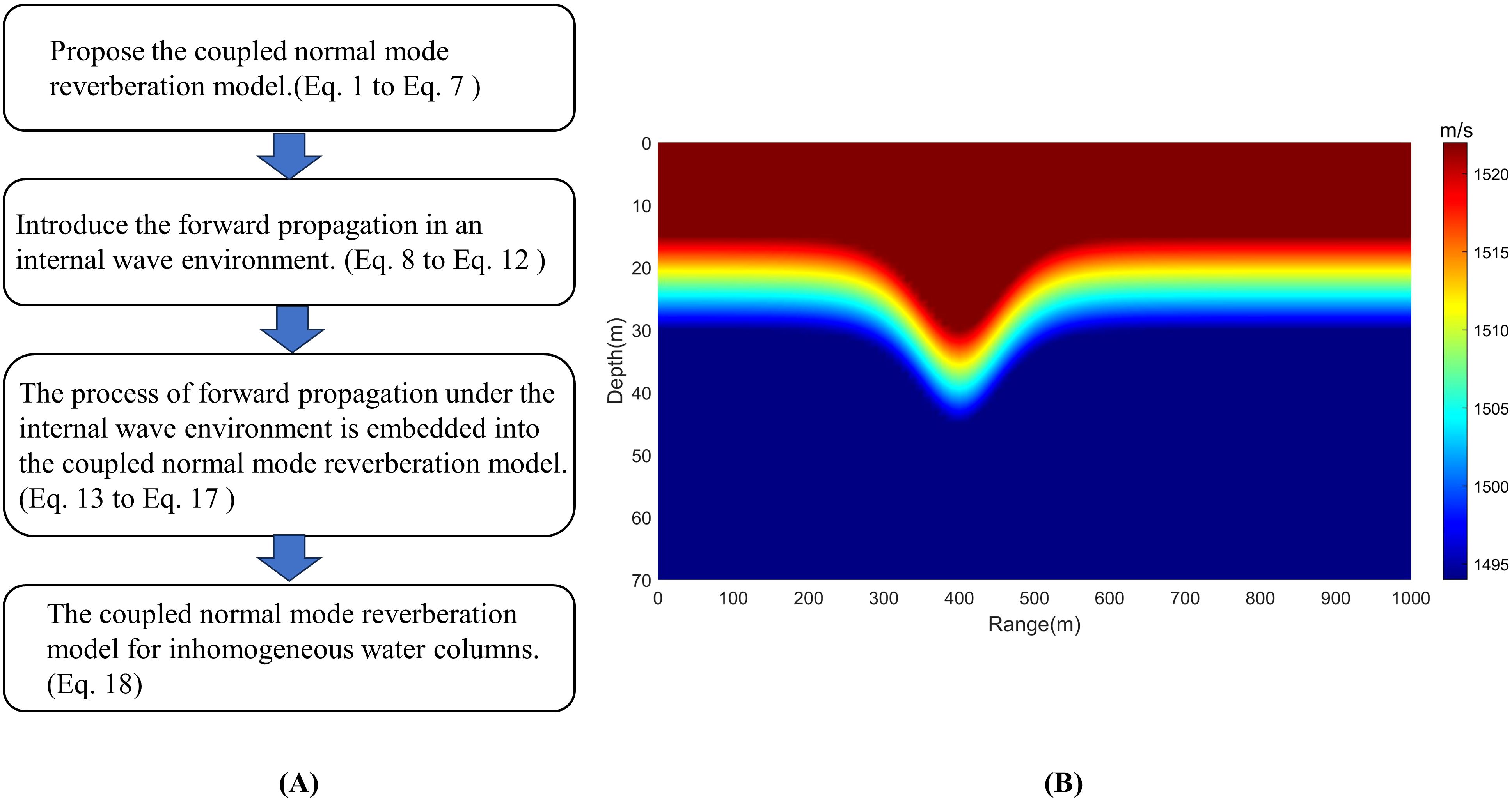
Figure 1. (A) The block diagram of this model. (B) Sound speed profile discussed in this study.

This study considers bottom reverberation in a two-layer medium with a rough bottom profile characterized by $H=H_0+\zeta (\overrightarrow{r})$, where $H_0$ is horizontal sea bottom depth and rough seabed fluctuation $\zeta$ is much smaller than $H_0$. The density and sound speed of the upper and lower layers are represented by ${\rho }_0$, $c_0$ and ${\rho }_1$, $c_1$, respectively, with b being the density ratio. $k_{rn}$ is the eigenvalue, $k_{0zn}$, and $k_{1zn}$ are the vertical wave numbers in the two media, defined as $k_{0zn}=\sqrt{k_0^2-k_{rn}^2}, k_{1zn}=\sqrt{k_1^2-k_{rn}^2}$. The pressure function $\phi (\overrightarrow{r})$, originating from a harmonic source at depth $z_s$, is defined as description in Yang (2010)’s Equation 4 and Gao et al (2010)’s Equation 1.

$\begin{array}{ll}\mathit{\phi }(\overrightarrow{\mathit{r}})=\sum _{\mathit{n}}{\psi }_n(\overrightarrow{\mathit{r}})Z_n(\mathit{z},k_{rn}).& (1)\end{array}$

where the local mode (vertical) function $Z_n$ is expressed as

$\begin{array}{ll}{Z}_n(\mathit{z},k_{rn})=\{\begin{array}{ll}{A}_{n}sin(k_{\mathbf{0}zn}z),\hfill & \mathit{z}\le \mathit{H}\hfill \\ A_{n}bsin(k_{\mathbf{1}zn}H){\mathit{e}}^{i{k}_{\mathbf{1}zn}(\mathit{z}-\mathit{H})},\hfill & \mathit{z}>\mathit{H}\hfill \end{array}& (2)\end{array}$

and

$\begin{array}{ll}{A}_n=\frac{\mathbf{2}i\pi sin(k_{\mathbf{0}zn}{z}_s)}{B_n}.& (3)\end{array}$

$\begin{array}{ll}{B}_n=\mathit{H}+\frac{({\mathit{k}}_{\mathbf{0}}^{\mathbf{2}}-k_{\mathbf{1}}^{\mathbf{2}})sin(\mathbf{2}{k}_{\mathbf{0}zn}H)}{(\mathbf{2}{k}_{\mathbf{0}zn}{k}_{1zn})}.& (4)\end{array}$

$\begin{array}{ll}\underset{\mathbf{0}}{\overset{\mathit{\infty }}{\int }}{Z}_n^{\mathbf{2}}(\mathit{z})dz=\frac{\mathbf{1}}{\mathbf{2}}{A}_n^{\mathbf{2}}\left\{B_n+\frac{(\mathit{b}-\mathbf{1})k_{\mathbf{0}zn}}{\mathbf{2}{k}_{\mathbf{1}zn}^{\mathbf{2}}}sin(\mathbf{2}{k}_{\mathbf{0}zn}H)\right\}={\Gamma }_{\mathit{n}}& (5)\end{array}$

Additionally, the element $G_{mn}$ of the coupled matrix $G$, which is applicable to a rough bottom, is defined as follows:

$\begin{array}{ll}{G}_{mn}=\int Z_n\frac{\partial Z_m}{\partial H}dz.& (6)\end{array}$

Given that bottom reverberation arises from first-order perturbations at the seabed interface, the horizontal function ${\psi }_n(\overrightarrow{r})$ is formulated as

$\begin{array}{ll}{\psi }_n(\overrightarrow{\mathit{r}})\approx \frac{\mathit{i}}{\mathbf{4}}{\displaystyle \iint {\mathit{H}}_{\mathbf{0}}^{(\mathbf{1})}}(k_{rn}\overrightarrow{\mathit{R}})\left[-\frac{\mathbf{2}{k}_{zn}^{\mathbf{2}}}{B_n}{\mathit{H}}_{\mathbf{0}}^{(\mathbf{1})}(k_{rn}\overrightarrow{\mathbf{r}\text{'}})\mathit{\zeta }+{\displaystyle \sum _{\mathit{m}}\frac{k_{rm}}{{\mathbf{\Gamma }}_n}{G}_{mn}}{\mathit{H}}_{\mathbf{1}}^{(\mathbf{1})}(k_{rm}\overrightarrow{\mathit{r}\text{'}})\left(\frac{\mathit{x}\text{'}}{\overrightarrow{\mathit{r}\text{'}}}\frac{\partial \zeta }{\partial x\text{'}}+\frac{\mathit{y}\text{'}}{\overrightarrow{\mathit{r}\text{'}}}\frac{\partial \zeta }{\partial y\text{'}}\right)\right]\mathit{d}\overrightarrow{\mathit{r}\text{'}}.& (7)\end{array}$

In the aforementioned equations, $\overrightarrow{r }$ represents the horizontal vector from the acoustic source to the receiver. The vector $\overrightarrow{r^{\prime }}$ signifies the horizontal vector from the acoustic source to the seabed scattering point. The vector $\overrightarrow{R}$ corresponds to the horizontal vector from the seabed scattering point to the receiver. Equation 7 characterizes the horizontal factor of the acoustic field’s potential function. Among them, $-\frac{2k_{zn}^2}{B_n}{H}_0^{(1)}(k_{rn}\overrightarrow{r^{\prime }})$ represents forward propagation, ${\sum }_m\frac{k_{rm}}{{\text{Γ}}_n}{G}_{mn}{H}_1^{(1)}(k_{rm}\overrightarrow{r^{\prime }})(\frac{x^{\prime }}{\overrightarrow{r^{\prime }}}\frac{\partial \zeta }{\partial x^{\prime }}+\frac{y^{\prime }}{\overrightarrow{r^{\prime }}}\frac{\partial \zeta }{\partial y^{\prime }})$ indicates modal coupling due to seabed fluctuations and $H_0^{(1)}(k_{rn}\overrightarrow{R})$ signifies backscattering. In addressing the influence of water column inhomogeneities, such as the presence of NIWs, adjustments must be applied to the vertical mode function $Z_n$. This necessitates the employment of mode coupling, as detailed by Yang (2014), to incorporate the water column’s coupling matrix. For the initial modeling of an NIW packet, we adopt the soliton solution of the Korteweg–de Vries (KdV) equation (Zheng et al., 2001), which is given by

$\begin{array}{ll}\widehat{\mathit{\eta }}=\mathbf{15}sec{h}^{\mathbf{2}}(\frac{\mathit{r}-r_x}{\mathit{\Delta }}).& (8)\end{array}$

In this context, the hyperbolic secant function is represented by sech, with $\widehat{\eta }$ signifying the amplitude of the NIW packet. The variable r corresponds to the horizontal coordinate, $r_x$ pinpoints the center position of the soliton, and Δ characterizes the width of the soliton.

In the modeling of pressure perturbations when the water column disturbs, the incident mode vector is characterized by Yang (2014)‘s Equation 2:

$\begin{array}{ll}\widehat{\mathit{A}}(\mathit{R})=\mathit{T}(R,r_{p+\mathbf{1}})\prod _{\mathit{k}=\mathbf{1}}^{\mathit{p}}\mathit{\Lambda }(r_{k+\mathbf{1}},r_k)\mathit{T}({\mathit{r}}_{\mathbf{1}},\mathbf{0})\widehat{\mathit{A}}(\mathbf{0}).& (9)\end{array}$

where $T(r_1,0)=diag\left\{e^{i{k}_r(r_1)}\right\}$ and $T(R,r_{p+1})=diag\left\{e^{i{k}_r(R-r_{p+1})}\right\}$ represent the mode propagation matrices. Here, $\widehat{A}(R)$ denotes the incident mode vector at a specific range R, while $\widehat{A}(0)$ is the source mode vector, which is associated with a standard eigenvector given by ${[{\phi }_1(z_s),{\phi }_2(z_s),\dots ,{\phi }_n(z_s)]}^H$ and is formulated as follows:

$\begin{array}{ll}\widehat{\mathit{A}}(\mathbf{0})=\frac{iexp(-i\pi /\mathbf{4}){\mathit{e}}^{-i\pi /\mathbf{4}}}{\sqrt{\mathbf{8}\mathit{\pi }}}{[{\mathit{\phi }}_{\mathbf{1}}(z_s),{\mathit{\phi }}_{\mathbf{2}}(z_s),\dots ,{\phi }_n(z_s)]}^{\mathit{H}}.& (10)\end{array}$

Within the mode coupling range from $r_k$ to $r_{k+1}$, the entry of the coupling matrix $\Lambda$ is expressed as:

$\begin{array}{ll}{\Lambda }_{nm}({\mathit{r}}_{\mathbf{2}},{\mathit{r}}_{\mathbf{1}})={\delta }_{nm}{\mathit{e}}^{i{k}_{rn}({\mathit{r}}_{\mathbf{2}}-{\mathit{r}}_{\mathbf{1}})}-i{S}_{nm}{\mathit{e}}^{\mathit{i}(k_{rn}{\mathit{r}}_{\mathbf{2}}-k_{rm}{\mathit{r}}_{\mathbf{1}})}-\frac{\mathbf{1}}{\mathbf{2}}\left({\displaystyle \sum _{\mathit{k}=\mathbf{1}}^{\mathit{M}}{S}_{nk}{S}_{km}}\right){\mathit{e}}^{\mathit{i}(k_{rn}{\mathit{r}}_{\mathbf{2}}-k_{rm}{\mathit{r}}_{\mathbf{1}})}+\cdots .& (11)\end{array}$

$\begin{array}{ll}{S}_{nm}=\frac{\mathbf{2}{k}_{rn}^{\mathbf{2}}}{\sqrt{k_{rn}{k}_{rm}}H}\int dzsin(k_{\mathbf{0}zn}z)sin(k_{\mathbf{0}zm}z)\times \underset{{\mathit{r}}_{\mathbf{1}}}{\overset{{\mathit{r}}_{\mathbf{2}}}{\int }}\frac{\delta c}{c_{\mathbf{0}}}{\mathit{e}}^{-\mathit{i}(k_{rn}-k_{rm})\mathit{r}}dr.& (12)\end{array}$

In the context of mode coupling, the element ${\Lambda }_{nm}$ within the range $r_k$ to $r_{k+1}$ is defined using the Kronecker delta ${\delta }_{nm}$, with $\delta c$ representing the speed perturbation induced by the NIW and $c_0$ being the ambient sound speed in the absence of NIWs.

The Sound Speed Profile (SSP) alteration due to NIWs is numerically computable, as demonstrated by Henyey and Tang (2013). The simulation employs an environmental model incorporating an NIW, depicted in Figure 1, to model an NIW packet as coherent structures traversing the acoustic path without deformation. Although the KdV equation-based mathematical model may not precisely describe the leading wave, the primary wave-packet is predominant in causing acoustic clutter, as highlighted by Henyey and Tang (2013), suggesting that the physical mechanisms and observed phenomena are analogous.

Subsequently, the mode coupling within the water column is integrated into the coupled mode reverberation theory. Traditionally, the coupled matrices in seabed reverberation theory are influenced solely by bottom roughness. The horizontal Hankel factor $H_0^{(1)}$ and the vertical eigenfunctions for the source $sin(k_{0zn}{z}_s)$ and receiver $sin(k_{0zn}z)$ are combined and derived into the vertical function $Z_n(z,k_{rn})$ and the horizontal function. When accounting for the inhomogeneous water column, these three terms are redefined within the incident mode vector $\widehat{\mathit{\text{A}}}(R)$, encapsulating the source’s eigenfunction and the Hankel function’s phase term, the receiver’s eigenfunction, and the spreading factor $\frac{1}{\sqrt{k_{rn}R}}$, which approximates the Hankel function’s amplitude. This framework facilitates a clear description of the coupling process within the incident mode vector $\widehat{\mathit{\text{A}}}(R)$.

Incorporating the NIW-induced incident mode coupling into the propagation of the coupled mode theory for seabed reverberation, the vertical function in Equation 2 is subsequently adjusted to reflect these considerations:

$\begin{array}{ll}{\widehat{Z}}_n(r,z,k_{rn})\approx \frac{\sqrt{\mathbf{2}}i\pi }{\sqrt{B_n}}{\widehat{A}}_n(r,z_s)sin(k_{0zn}z)e^{-i{k}_{rn}r},\mathit{z}\le \mathit{H}.& (13)\end{array}$

where ${\widehat{A}}_n(r,z_s)$ denotes the n-th component of the incident mode vector $\widehat{\mathit{\text{A}}}(R)$ as defined by Equation 9. The horizontal function ${\psi }_n(\overrightarrow{r})$ retains the form given in Equation 7. Meanwhile, the element ${\widehat{G}}_{mn}$ of the coupled matrix $\widehat{G}$, as presented in Equation 8, is transformed to become

$\begin{array}{ll}{\widehat{G}}_{mn}(\mathit{r})\approx \frac{-\mathbf{2}{\mathit{\pi }}^{\mathbf{2}}{\mathit{e}}^{-\mathit{i}(k_{rm}+k_{rn})\mathit{r}}{\widehat{A}}_m(\mathit{r}){\widehat{A}}_n(\mathit{r})}{\sqrt{B_m{B}_n}}\underset{0}{\overset{\infty }{\int }}sin(k_{0zn}z)\frac{\partial sin(k_{0zm}z)}{\partial H}dz.& (14)\end{array}$

Consequently, the pressure function $\widehat{\phi }(\overrightarrow{r})$, as indicated in Equation 1, can be reformulated as follows:

$\begin{array}{ll}\widehat{\mathit{\phi }}(\overrightarrow{\mathit{r}})=\sum _{\mathit{n}}{\psi }_n(\overrightarrow{\mathit{r}}){\widehat{Z}}_n(z,k_{rn})& (15)\end{array}$

During the numerical simulation, Equation 7 is utilized to calculate the Reverberation Level (RL). To simplify the scenario, a mono-static condition is assumed, and the partial derivative of the isotropic roughness $\zeta$ is taken as zero and transformed the area integration into line integration. This leads to the following expression:

$\begin{array}{ll}{\psi }_n\approx \frac{-\mathit{i}}{\mathbf{4}}{\displaystyle \iint \frac{\mathbf{2}{k}_{zn}^{\mathbf{2}}}{B_n}}{\mathit{H}}_{\mathbf{0}}^{(\mathbf{1})}(k_{rn}\overrightarrow{\mathit{R}}){\mathit{H}}_{\mathbf{0}}^{(\mathbf{1})}(k_{rn}\overrightarrow{\mathit{r}\text{'}})\mathit{\zeta }\mathit{d}\overrightarrow{\mathit{r}}=i\pi {\displaystyle \int \frac{k_{zn}^{\mathbf{2}}}{B_n}}{\left[{\mathit{H}}_{\mathbf{0}}^{(\mathbf{1})}(k_{rn}\overrightarrow{\mathit{r}})\right]}^{\mathbf{2}}\mathit{\zeta }(\overrightarrow{\mathit{r}})\overrightarrow{\mathit{r}}\mathit{d}\overrightarrow{\mathit{r}}.& (16)\end{array}$

Furthermore, Equation 15 is expanded to its full form as follows:

$\begin{array}{ll}\widehat{\mathit{\phi }}(\overrightarrow{\mathit{r}})=-i\pi \sum _n{\widehat{Z}}_n(z,k_{rn})\int \frac{k_{zn}^{\mathbf{2}}}{B_n}{\left[{\mathit{H}}_{\mathbf{0}}^{(\mathbf{1})}(k_{rn}\overrightarrow{\mathit{r}})\right]}^{\mathbf{2}}\mathit{\zeta }(\overrightarrow{\mathit{r}})\overrightarrow{\mathit{r}}\mathit{d}\overrightarrow{\mathit{r}}.& (17)\end{array}$

Thus, an amended expression for the RL that accounts for the presence of NIWs is derived as Equation 18.

$\begin{array}{ll}RL(\overrightarrow{\mathit{r}})=\widehat{\mathit{\phi }}(\overrightarrow{\mathit{r}},z_s,z_r){\widehat{\mathit{\phi }}}^{*}(\overrightarrow{\mathit{r}},z_s,z_r)& (18)\end{array}$

3 Simulation results

3.1 Numerical simulation of the reverberation model

The modeled sound speed profile (SSP) corresponds to a typical summer condition in the Yellow Sea of China, characterized by a pronounced thermocline between 15 to 25 m depths, as shown in Figure 1B. The seafloor is presumed to be a fluid half-space with a sound speed of 1700 m/s, a density ratio of 1.6, and an attenuation of 0.4 dB per wavelength. The waveguide depth is set at 70 m, with the sound source positioned 35 m below the thermocline.

Figure 2A depicts the coupling matrix $\text{Λ}(r_2,r_1)$, which is influenced by the environmental parameters of the internal wave packets, including the soliton wave amplitude $\widehat{\eta }$ and the horizontal extent $\text{Δ}=r_3-r_1$. As the acoustic signal traverses from $r_1$ to $r_2$, through the core of the NIW, the mode coupling effects intensify, leading to the generation of higher modes and a significant increase in clutter above the background reverberation level. At location $r_3$, some higher modes vanish, causing a swift decrease in clutter intensity after peaking. (Figures 2B–D) illustrate the mode coupling mechanism using a 3000 Hz continuous wave (CW) signal.

Figure 2

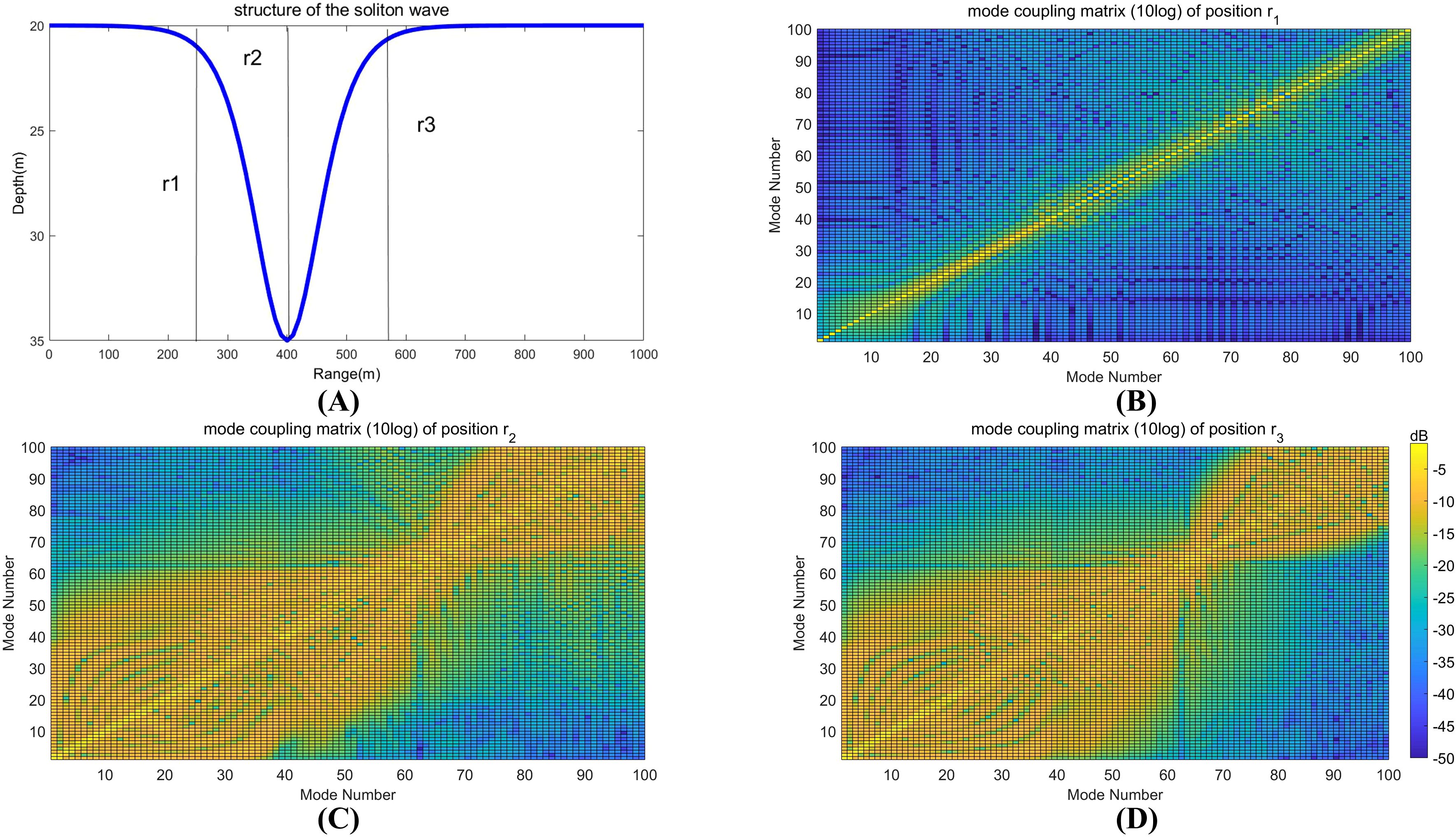
Figure 2. (A) Geometry of the NIW, (B–D) showing energy redistributed at three different positions (i.e., position r_1, r_2, and r₃) when the acoustic signal propagates through the NIW. Only the first 100 modes are presented in the simulated results.

Under identical internal wave conditions, the mode coupling among the initial 80 normal modes of a 2000 Hz CW signal is simulated across four scenarios: not passing through the internal wave (Figure 3A), just entering the internal wave (Figure 3B), preparing to move away from the internal wave (Figure 3C), and fully moving away from the internal wave (Figure 3D). The results indicate that, under various frequency signals, the coupling between normal modes is enhanced as the signal moves from $r_1$ to $r_2$. Some higher modes disappear at $r_3$, but many higher-order modes persist compared to pre-internal wave conditions.

Figure 3

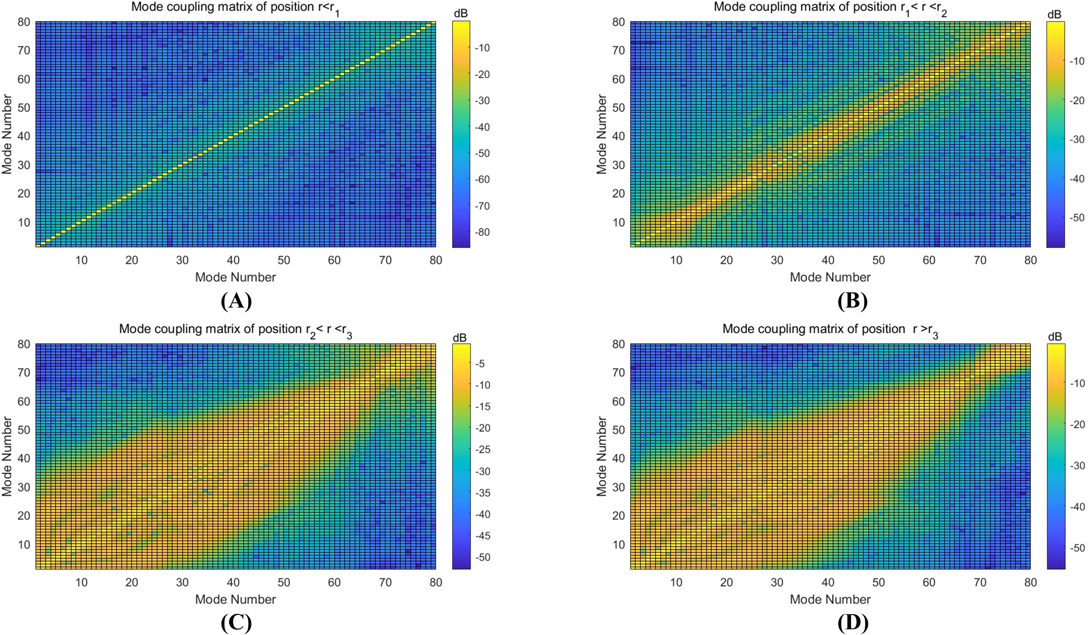
Figure 3. (A–D) showing energy redistributed at four different positions when the 2000 Hz CW signal propagates through the NIW. Only the first 80 modes are presented in the simulated results.

To further elucidate the internal wave’s impact on the coupling matrix, simulations were conducted with two internal wave packets (Figure 4A). Subsequent figures (Figures 4B–D) display the coupling matrices for a 2000 Hz CW signal traversing these internal waves, revealing that numerous higher-order modes remain excited even after completely passing through the internal wave packets.

Figure 4

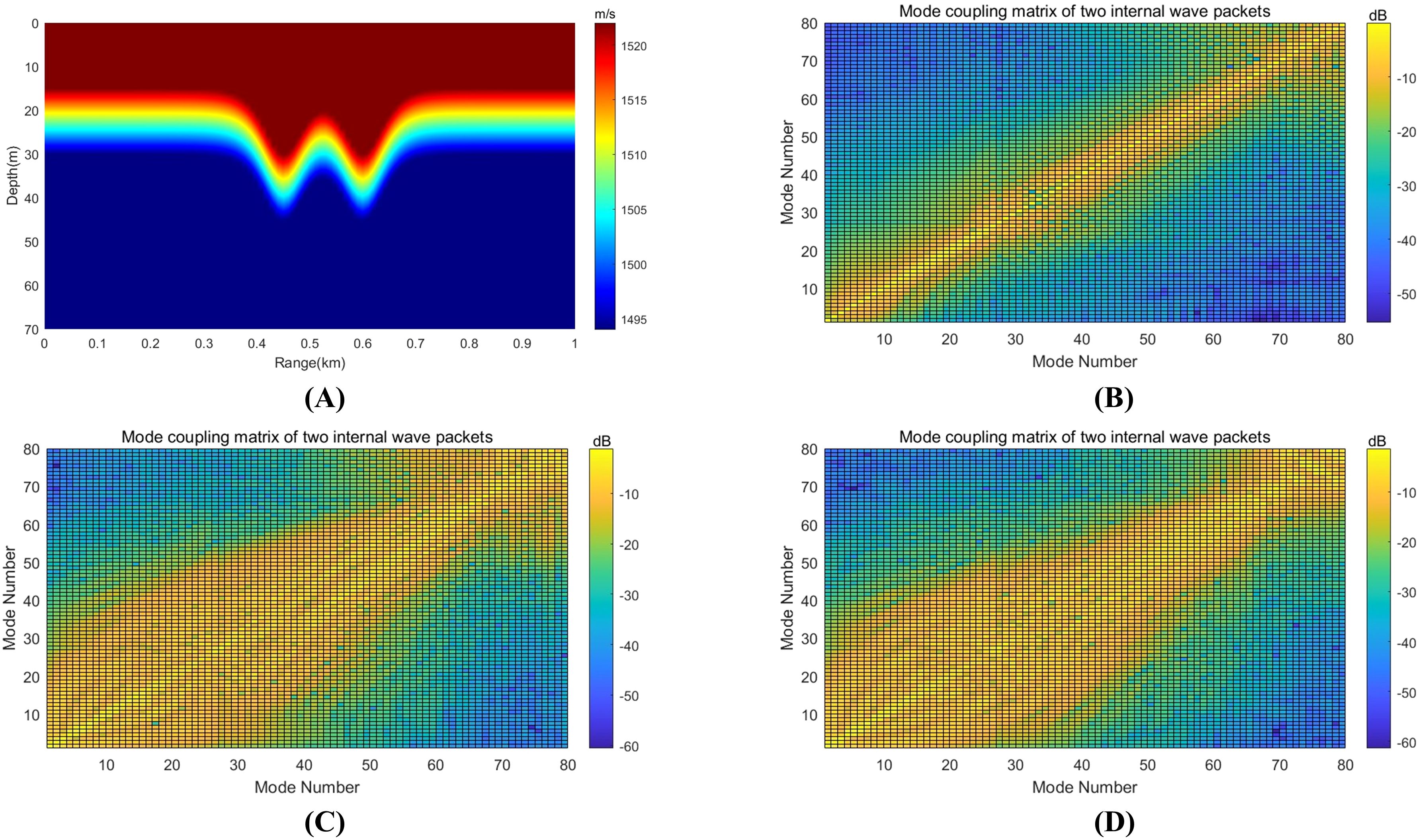
Figure 4. (A) Simulated sound speed profile of two internal wave packets, (B–D) showing energy redistributed at four different positions when the 2000 Hz CW signal propagates through the two internal wave packets. Only the first 80 modes are presented in the simulated results.

Figure 5A presents the coherent reverberation level (CRL) curves that demonstrate the emergence of target-like clutter at the 4 s mark, corresponding to the NIW’s position at 3 km. The solid line represents the time-averaged RL calculated over a 0.1 s window, while the dashed line corresponds to the incoherent reverberation level (IRL). Figure 5B displays IRL curves for various NIW positions. In comparison to the baseline RL without NIWs (indicated by the blue dashed-dotted line), using the traditional normal mode reverberation model, pronounced peaks, roughly 10 dB above the background level, appear at distinct times for each NIW position. Compared with the traditional normal mode reverberation model, the introduction of the coupling matrix allows for a more nuanced depiction of the influence of internal waves on the reverberation curve.

Figure 5

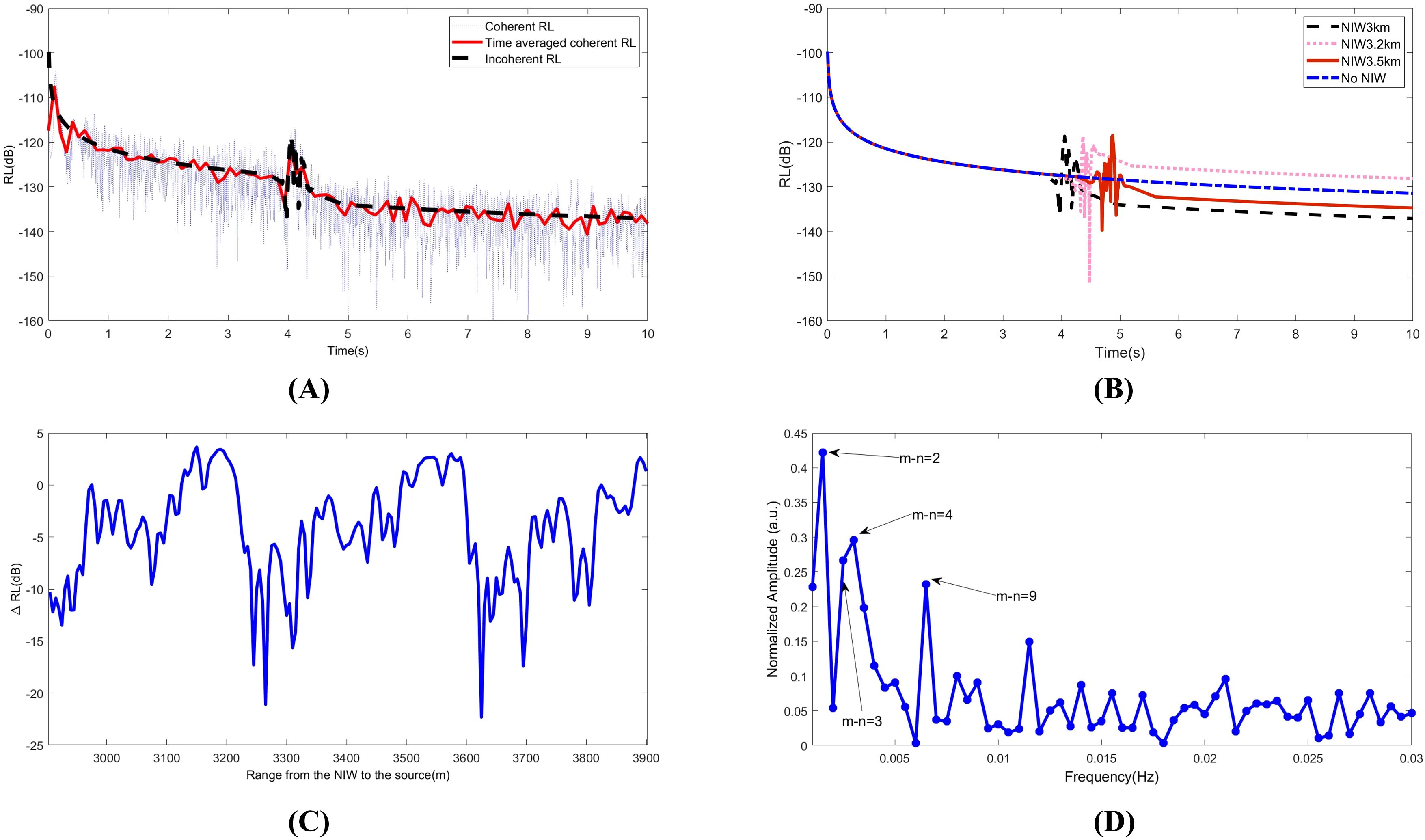
Figure 5. (A) Simulated coherent RL (dotted line) when the distance between a source and the NIW is 3 km; the solid line denotes the time-averaged coherent RL, and the dashed line represents the incoherent RL. (B) Incoherent RL curves for the source-NIW distance of 3 (dashed line), 3.2 (dotted line), and 3.5 (solid line) km, respectively; in the absence of an NIW, using traditional reverberation model, the RL is represented by the dashed-dotted line. (C) Fluctuation of RL at 6 s, when a soliton moves with the speed of 0.5 m/s, and the distance between source and NIW is changed from 3 to 4 km. (D) Normalized spectrum of the time series shown in (C); the spectral peaks indicated by arrows show the dominant mode number differences.

During the analysis of actual data, an appropriately chosen time-averaged window is commonly employed to derive the IRL curve. The consistency between the time-averaged CRL and IRL, as depicted in Figure 5A, validates this approach.

From the simulation results, it can be concluded that as the sound wave initially enters the range of internal waves, the hydrological environment changes, and energy begins to transfer to higher-order normal modes. When the sound wave continues to propagate into the center of the internal wave, the hydrological environment changes most intensely, with a strong energy transfer to higher-order normal modes. After the sound wave has completely passed through the internal wave, a large number of high-order modal normal modes appear. Along the forward propagation path, due to the inhomogeneity of the water columns, a strong coupling effect occurs, transferring a significant amount of energy to higher-order modes, increasing the grazing angle of the seabed reverberation, and enhancing the seabed scattering intensity, thus leading to the emergence of strong clutter. Based on the normal mode reverberation model, the analysis of the coupling matrix can detail the modal coupling caused by the inhomogeneity of the water columns, providing a clearer expression of the energy transfer of each normal mode within the internal wave, and demonstrating the physical mechanism by which internal waves cause the generation of clutter.

Equation 18 represents the product of two summation terms. In terms of matrix multiplication, the sum of the diagonal elements corresponds to the incoherent reverberation level (IRL), aligning with Ellis (1995)’s Equation 14. Meanwhile, the sum of the off-diagonal elements is identified as the coherent reverberation level (CRL), consistent with Ellis (1995)’s Equation 15. The traditional normal mode reverberation model is designed for horizontally stratified media. However, the modified expression in Equation 17 remains applicable to non-horizontally stratified water columns. This is due to $A_n(r)$, which encapsulates the mode coupling process and reflects the dynamic changes in modal amplitudes caused by NIWs. Such adaptability is a key strength of the revised model presented in this paper.

Additionally, the model we propose can provide a unified modeling approach for complex sound speed gradients and seabed reverberation. Furthermore, for traditional reverberation models of horizontally stratified and horizontally gently varying waveguides, the introduction of the coupling matrix allows for more convenient generalization; it simply requires focusing the coupling energy, like other methods, on the off-diagonal elements. In summary, this model expands the scope of ocean reverberation modeling.

3.2 Fluctuation of RL after clutter arrival

An intriguing phenomenon observed in Figure 5B is that the RL following the peak values significantly deviates from the extrapolated baseline prior to the internal wave’s arrival. Furthermore, this RL variation is closely tied to the movement of the NIW. Although this effect was reported by Henyey and Tang (2013), the mechanism behind it is not yet clear.

To investigate this mechanism, the NIW shown in Figure 1 was considered to be moving away from the source at a speed of 0.5 m/s. A series of two hundred 3 kHz frequency signals were transmitted at 10 s intervals over a period of 2000 s. The distance between the NIW and the source was altered from 3 to 4 km, with the target-like arrival time calculated to range between 4 to 5.33 s. The reverberation observation time was fixed at 6 s to ensure that the NIW was situated between the source and the scattering area. The IRLs were defined as the 200 IRLs at 6 seconds affected by the moving NIW, denoted as $IR{L}_s$, while $IR{L}_0$ represented the IRL at 6 s in the scenario without an NIW. Thus, the time series of $\text{Δ}IR{L}_s= IR{L}_s- IR{L}_0$ consisted of 200 data points, capturing the dynamic changes in reverberation levels.

The calculated result is shown in Figure 5C. Evidently, the fluctuation of $\text{Δ}IRL$ exhibits a quasi-periodic structure and does not follow a simple harmonic oscillation. To explain this, a Fourier analysis of the time series $\text{Δ}IR{L}_s$ was performed, and the resulting normalized spectrum is shown in Figure 5D. The dominating spectral peaks matched well with the mode wavenumber differences, that is, with $f_{mn}=v{k}_{mn}/2\pi$, where $k_{mn}=k_m-k_n$, and v is the speed of the moving NIW. This can be identified based on the propagation effect owing to the mode coupling caused by the moving NIW. The NIW packet caused mode coupling and their motion resulted in a changing acoustic interference pattern of reverberation intensity. Similar effects have been reported in the propagation problem in presence of NIWs and experimentally observed in the SWARM experiment (Duda and Preisig, 1999). To the best of the authors’ knowledge, no study has reported that a similar effect can occur in RL in the presence of moving NIW packets; This also explains the observation in Henyey and Tang (2013). Moreover, the result in Henyey and Tang (2013) is simply a special case of the general fluctuation discussed in this study.

4 Experimental verification

A shallow-water reverberation experiment was conducted in the North Yellow Sea from July 8 to 10, 2014. The water depth averaged 45 m, with a low-frequency transducer deployed at a depth of 22 m serving as the sound source. A vertical line array (VLA), comprising 16 element pressure hydrophones, was used to receive the signals. The hydrophones were spaced 3 meters apart, and both the sound source and the VLA were situated on the same vessel to establish a monostatic reverberation testing configuration. Environmental measurements indicated bottom parameters of ${\rho }_2$ = 1850 $kg/m^3$ and $c_2$ = 1770 m/s. A variety of signals, including CW and Chirp signals, were transmitted starting at noon local time on July 8th.

The purpose of the experiment was to explore the impact of internal waves on shallow-water reverberation. To effectively monitor internal waves, two temperature chains equipped with 16 temperature and depth (TD) sensors each were deployed near the research vessel, with sensors spaced 0.5 m apart. These TD sensors, measuring 150 mm in length and 40 mm in diameter, were capable of measuring temperatures ranging from -2°C to 40°C. The chains were anchored perpendicular to the isobaths, considering that the propagation of NIWs is generally aligned with the isobaths’ vertical direction and influenced by tidal forces. This arrangement ensured that soliton waves, akin to plane waves, would sequentially pass through both temperature chains.

The first temperature chain (Tc-A) was positioned 723 m from the vessel, North Survey I, which has a displacement of 1200 tons, while the second chain (Tc-B) was 1037 m away. The vessel was anchored roughly midway between the two chains. Figure 6A and Figure 6B illustrate a series of NIWs detected by Tc-A and Tc-B. Despite some packets’ shapes changing as they propagated, the initiation point of each packet allowed us to determine that the propagation time across both temperature chains was approximately 1.5 hours (5400 s), with a distance of 1760 m between Tc-A and Tc-B. Consequently, the speed of the soliton wave was calculated to be $v_r$ = 0.325 m/s, which aligns with historical data of internal wave speeds in the northern Yellow Sea, ranging from 0.3 m/s to 0.4 m/s (Hu et al., 2020).

Figure 6

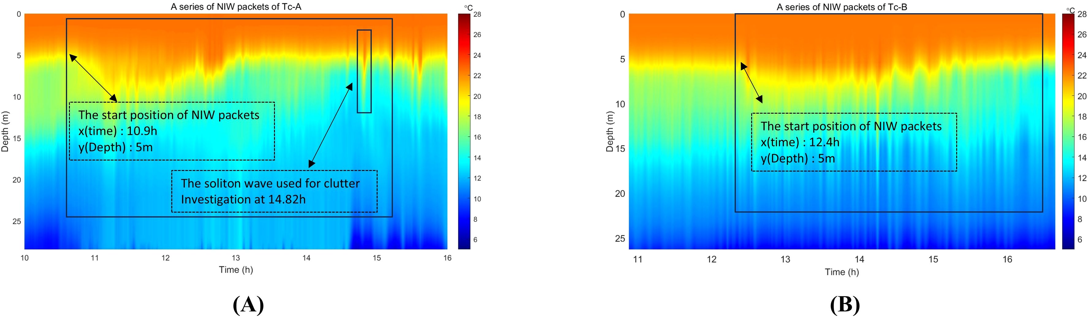
Figure 6. (A) showing the recorded temperature data of the experimental area from Tc-A. (B) showing the recorded temperature data of the experimental area from Tc-B.

A pronounced soliton wave, identified from the sequence of the NIW packets in Figure 7A, was selected for analyzing the clutter effects. This wave was recorded by Temperature Chain-A (Tc-A) at 14.82 hours after noon, as depicted in Figure 7A. Concurrently, at 14.115 hours after noon, a series of CW signals, each 0.2 s in duration, were emitted. The reverberation intensity captured by the 8th, 11th, and 12th hydrophones is displayed in Figure 7B, revealing the emergence of target-like clutter at 2.047s.

Figure 7

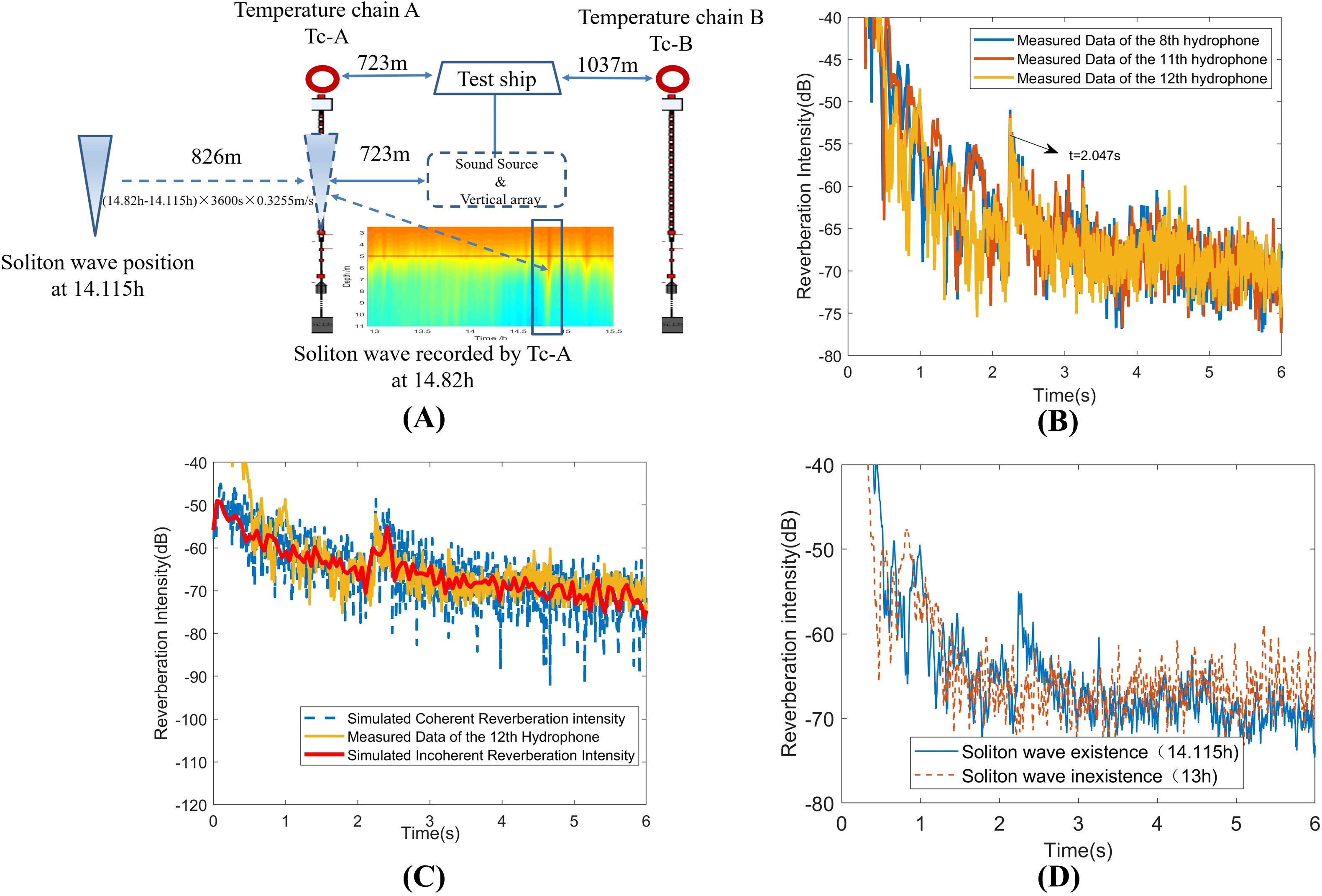
Figure 7. (A) Diagram of clutter induced by the soliton wave. (B) Collected data of reverberation and clutter induced by the soliton wave at the time 14.115 h after the start of the experiment. (C) Comparison between the numerically simulated calculations and the measured clutter data. (D) Comparison between the measured reverberation clutter data with soliton wave existence and soliton wave in nonexistence.

The internal wave illustrated in Figure 7A is capable of inducing clutter in the signals received by the test ship. With the soliton wave’s speed established at 0.325 m/s, the distance from the wave to the sound source at 14.115 hours was approximately 1549 m (723 + 826 m). According to the theoretical calculations based on Equation 18, the clutter was expected to appear at a time of $\frac{1549m\times 2}{1500m/s}=2.065s$.

As indicated in Figure 7C, the theoretical clutter appearance time of 2.065 seconds closely matches the measured time of 2.047 s. A minor discrepancy between the theoretical and measured clutter intensities is observed, attributable to the lack of a second temperature chain to verify the soliton wave’s precise structure at the 1549 m mark from the ship during the signal transmission at 14.115 hours. The theoretical model’s soliton wave structure is inferred from the Tc-A data recorded at 14.82 hours. Despite the half-hour time difference, the soliton wave’s structure is expected to have undergone slight changes, which is the primary source of the mismatch. Notably, by the time this strong soliton wave reached Tc-B after 1.5 hours, its amplitude had altered significantly, as evident from Figure 6B. Initially, the authors were uncertain about the reliability of estimating the soliton wave structure at 14.115 hours, but the comparison in Figure 7C confirms the estimation’s accuracy. Furthermore, by analyzing data from various time points, it can be deduced that internal waves can induce the generation of clutter, as illustrated in Figure 7D.

It is important to clarify that the clutter is not a result of direct reflection of underwater acoustic wave by the soliton wave. Instead, the clutter effect leads to enhanced mode coupling within the forward-propagating sound field. This implies that energy from lower modes (with lower incident grazing angles) is transferred to higher modes (with higher grazing angles). Notably, another set of solitary internal waves was detected by Tc-A at 16.5 hours, as shown in Figure 8A. At 16.27 hours, the test vessel emitted 30 sets of single-frequency signals, each consisting of ten pulses with widths of 0.2 s, 0.5 s, and 1.0 s, at a frequency of 580 Hz.

Figure 8

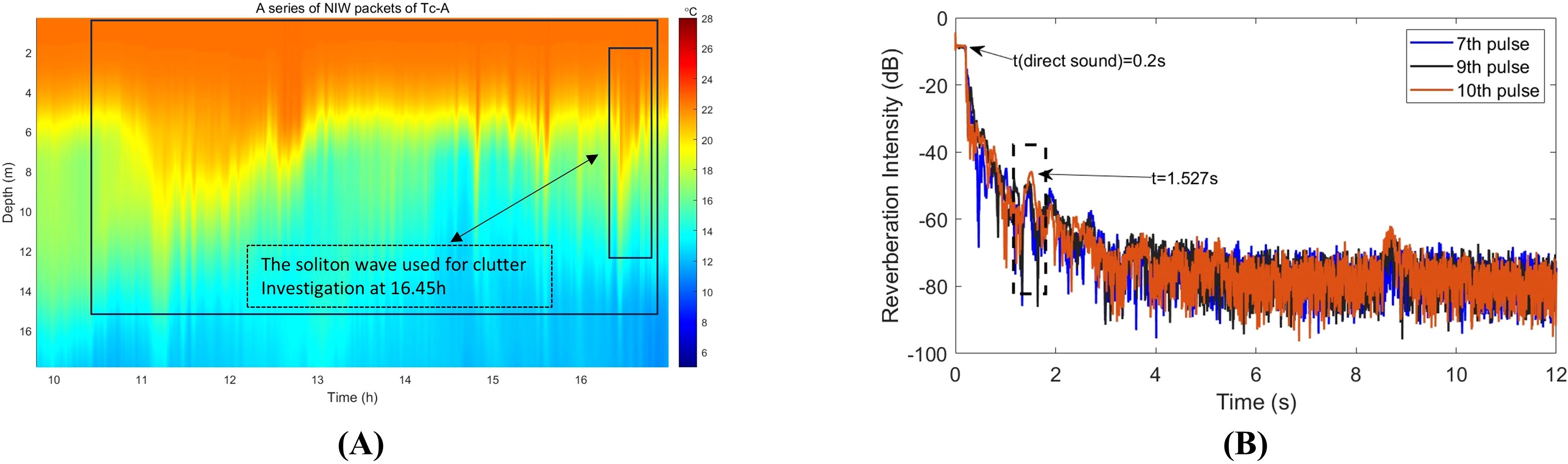
Figure 8. (A) showing another set of solitary internal waves was detected by Tc-A at 16.5 hours, and (B) showing pulses 7, 9, and 10 of a 580 Hz 0.2 s pulse reverberation signal intensity attenuation.

At the time of observation, the solitary internal wave was positioned 210.9 m from Tc-A. Based on the established speed of internal waves in the region, the anticipated arrival time of the clutter was determined to be 1.245 s. The testing vessel transmitted a 580 Hz signal, and the data from the 9th hydrophone, located at a depth of 19.5 m, were analyzed, as illustrated in Figure 8B. The clutter was detected at 1.527 s; after accounting for the direct sound travel time of 0.2 s, the clutter’s actual occurrence time was 1.327 s. This aligns well with the predicted clutter time of 1.245 s, resulting from the internal wave’s influence, with a minor discrepancy of 0.082 s. Figure 8B shows that, at this depth, clutter associated with different pulse widths (0.2 s, 0.5 s, 1.0 s) of the CW signal is observable at the expected time intervals, verifying that the clutter was indeed induced by the moving solitary internal wave.

For the analysis of reverberation data with clutter occurrences at different pulse widths, data segments corresponding to 0.2 s, 0.5 s, and 1.0 s pulse durations were examined. As depicted in Figure 9, for the (A) 0.2 s pulse width, the theoretical prediction for clutter induction by the internal wave was at 1.2074 s, with the actual measurement at 1.2045 s, yielding a negligible error of 0.0029 s. For the (B) 0.5 s pulse width, the calculated clutter time was 1.1289 s, and the measured time was 1.1254 s, with a slight error of 0.0035 s. Lastly, for the (C) 1.0 s pulse width, the expected clutter time was 0.9136 s, against an observed time of 0.9733 s, resulting in a larger discrepancy of 0.0597 s.

Figure 9

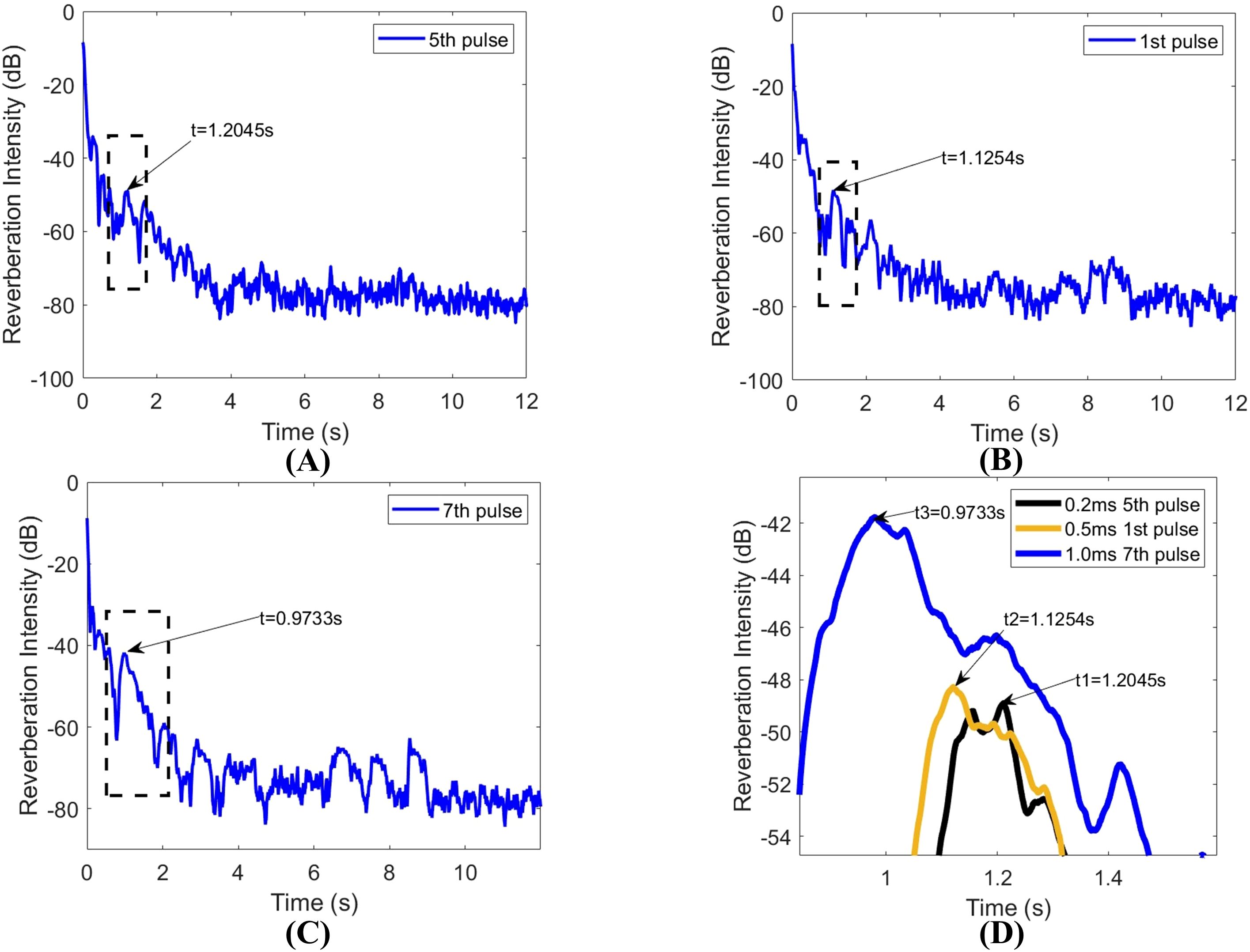
Figure 9. (A–C) showing reverberation data with the proper clutter appearance time, and (D) showing the “drift” phenomenon.

When plotting these three curves together, it becomes evident that the clutter position shifts as the internal wave moves, a movement referred to as the “drift” phenomenon, as shown in Figure 9D.

In conjunction with the theoretical framework from Section 2, the reverberation signals from 30 sets of 580 Hz single-frequency transmissions, influenced by the moving internal waves at the specified depth, were averaged at a fixed time. The difference from reverberation signals not affected by the internal waves was calculated to ascertain the change in reverberation intensity at the time of observation. Time-domain interpolation was applied to the intensity change data based on the transmission timing, creating a time-domain reverberation intensity change curve spanning 846 s. A Fourier transform was subsequently applied to convert this into the frequency domain, revealing how the reverberation intensity changes over various time spans.

The relationship between the frequency $f_{mn}$ and the horizontal wavenumber $k_{mn}$ is given by $f_{mn}=v_r{k}_{mn}/2\pi$, which can be rearranged to $k_{mn}=\frac{2\pi f_{mn}}{v_r}$, where $v_r$ denotes the velocity of the internal wave. The empirical value of $k_{mn}$ was found to be $19.3\times f_{mn}$.

The time-domain and frequency-domain representations of the reverberation signal, processed with a 0.2 s window, were generated using data from 6.0 s to 6.2 s and from 6.3 s to 6.5 s.

The reverberation signals depicted in Figures 10A and 10B were captured between 6.0 and 6.2 s. These signals are associated with the horizontal wave numbers as simulated by the Kraken model, detailed in Table 1.

Figure 10

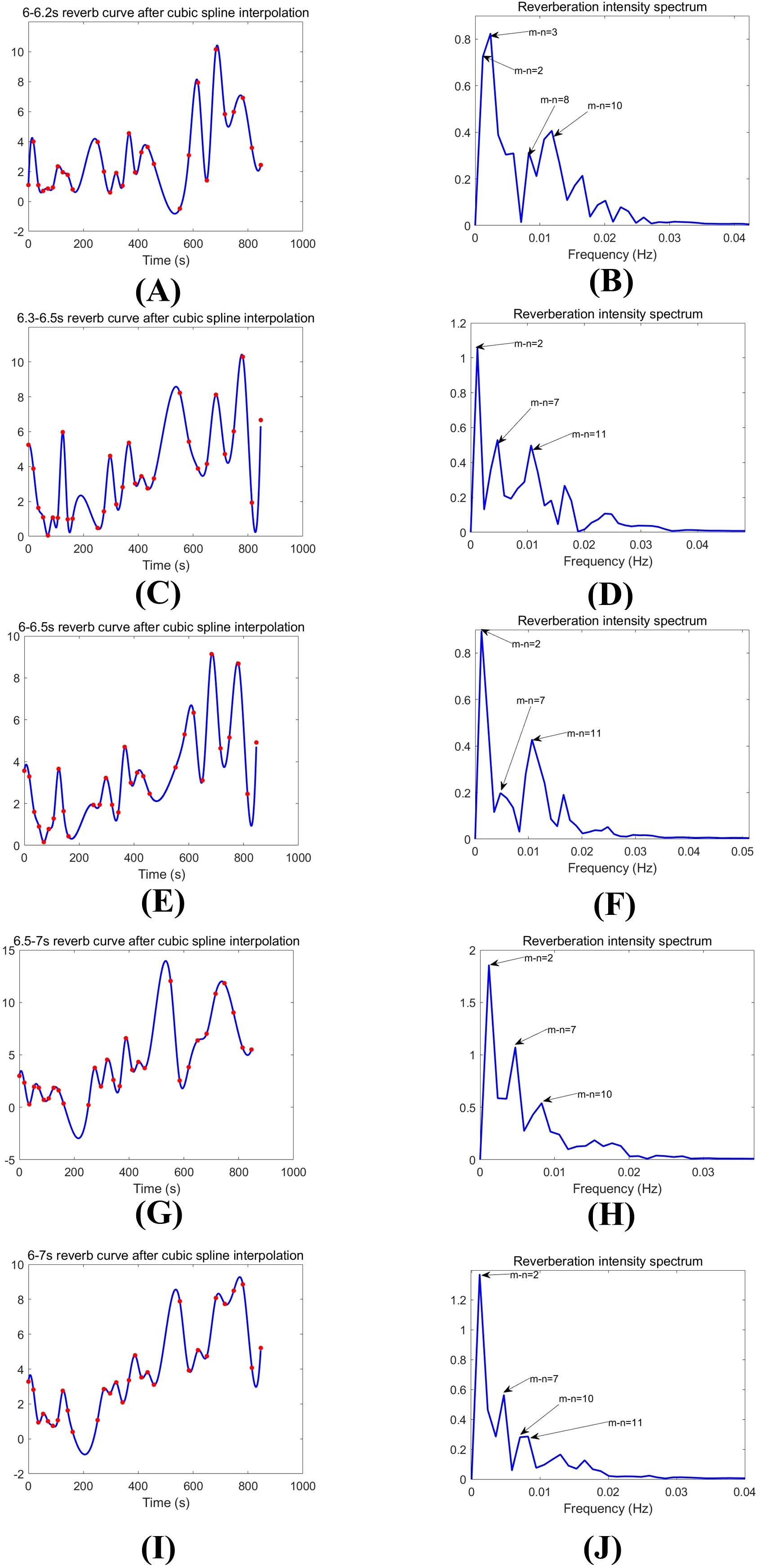
Figure 10. (A, B) showing the time-domain and frequency-domain of the average reverberation signal from 6-6.2s; (C, D) showing the time-domain and frequency-domain of the average reverberation signal from 6.3-6.5s; (E, F) showing the time-domain and frequency-domain of the average reverberation signal from 6-6.5s; (G, H) showing the time-domain and frequency-domain of the average reverberation signal from 6.5-7s; (I, J) showing the time-domain and frequency-domain of the average reverberation signal from 6-7s.

Table 1

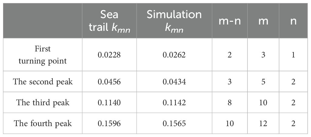
Table 1. The comparison of sea trials and simulation k_mn within the time window of 6.0 s to 6.2 s.

Figure 10C and Figure 10D display the reverberation signals recorded in the time interval from 6.3 to 6.5 s. These signals correspond to the horizontal wave numbers as simulated by the Kraken model, with the specific values and comparisons provided in Table 2.

Table 2

Table 2. The comparison of sea trials and simulation k_mn within the time window of 6.3 s to 6.5 s.

The reverberation signals presented in Figures 10E and 10F were obtained using a 0.5-second time window, with the data extracted from the time span of 6.0 to 6.5 s. These signals are aligned with the horizontal wave numbers from the Kraken simulation, as detailed in Table 3. Additionally, the reverberation signals from 6.5 to 7.0 s, processed with the same time window, are also considered as part of the analysis.

Table 3

Table 3. The comparison of sea trials and simulation k_mn within the time window of 6.0 s to 6.5 s.

Figures 10G and 10H illustrate the reverberation signals acquired between 6.5 and 7.0 s. These signals are matched with the horizontal wave numbers from the Kraken simulation results, which are detailed in Table 4.

Table 4

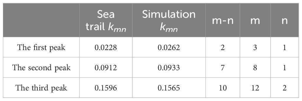
Table 4. The comparison of sea trials and simulation k_mn within the time window of 6.5 s to 7.0 s.

The reverberation signals depicted in Figures 10I and 10J were processed using a 1.0 s window and were extracted from the time interval ranging from 6.0 to 7.0 s. These signals correspond to the horizontal wave numbers obtained from the Kraken simulation, as presented in Table 5.

Table 5

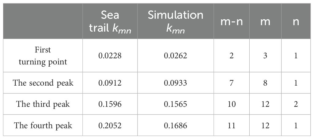
Table 5. The comparison of sea trials and simulation k_mn within the time window of 6.0 s to 7.0 s.

The analysis, in conjunction with the simulation experiment, reveals that the principal frequency component of the reverberation intensity oscillation at a constant observation time is correlated with the interference interval between a pair of normal waves.

Thus, it can be demonstrated from the correspondence between data processing and simulation results that internal wave imprint target information on the reverberation curve, and that internal wave velocity can be extracted from the reverberation oscillations in the frequency domain. Compared with traditional methods of measuring internal wave speeds, using reverberation to extract internal wave velocity eliminates the need for high-cost ADCP transect testing using high-frequency signals, as well as traditional long-term fixed-point observations by buoys and extensive SAR data inversion. This approach offers more proactive, intuitive, and convenient features, with lower implementation costs, requiring only a transmit-receive sonar. By utilizing reverberation, which is traditionally regarded as interference in active sonar, the detection of internal waves is achieved.

5 Discussion

This research conducted a shallow-water reverberation and clutter experiment in the northern Yellow China Sea in July 2014, focusing on the analysis of clutter caused by NIWs through reverberation data. The findings confirm that the soliton wave’s movement is indicative of target-like clutter, as evidenced by the wave’s temporal progression. Theoretical insights were gained by applying the coupled-mode approach (Yang, 2014) to calculate and interpret the reverberation and clutter dynamics with a moving NIW. The simulations indicated that NIWs, particularly those with substantial amplitude, generate significant and target-like reverberation clutter, corroborating the observations by Henyey and Tang (2013). The study also highlighted the quasi-periodic oscillation in reverberation intensity following the clutter, which is influenced by the soliton’s motion. The Fourier spectrum analysis of these oscillations revealed primary peaks that aligned with the mode-coupling theory’s predictions, suggesting a dependency on the NIW’s position. The main frequency of reverberation oscillation during fixed observation periods was found to be linked to the velocity of the internal wave movement. While this study offers plausible explanations, further validation is necessary using more refined experimental data.

Data availability statement

The datasets presented in this article cannot be publicly shared due to privacy restrictions. Requests to access the datasets should be directed to the corresponding author.

Author contributions

BG: Methodology, Supervision, Writing – original draft. GL: Data curation, Writing – review & editing. JP: Software, Writing – original draft.

Funding

The author(s) declare financial support was received for the research, authorship, and/or publication of this article. This work was supported by the National Natural Science Foundation of China (12374427)

Acknowledgments

The authors would like to express their great appreciation to Professor Ning Wang for his support and helpful comments. The authors also thank Professor Jinrong Wu for providing the high-quality data that was used to calibrate our calculations.

Conflict of interest

The authors declare that the research was conducted in the absence of any commercial or financial relationships that could be construed as a potential conflict of interest.

Publisher’s note

All claims expressed in this article are solely those of the authors and do not necessarily represent those of their affiliated organizations, or those of the publisher, the editors and the reviewers. Any product that may be evaluated in this article, or claim that may be made by its manufacturer, is not guaranteed or endorsed by the publisher.

Supplementary material

The Supplementary Material for this article can be found online at: https://www.frontiersin.org/articles/10.3389/fmars.2024.1410399/full#supplementary-material

References

Chen Y., Yu F., Zhang. L., Wang. F., Liu Q., Jiang B., et al. (2020). Design and development of deep-sea buoys and their applications in the tropical western Pacific. Mar. Science. 44, 215–222. doi: 10.11759/hykx20200327005

Crossref Full Text | Google Scholar

Chong J., Zhou X. (2013). Survey of study on internal waves detection in synthetic aperture radar image. J. Radars 2, 406–421. doi: 10.3724/SP.J.1300.2013.13012

Crossref Full Text | Google Scholar

Chun M., Leng S., Liang S., Wang Z., Luo X., Yang X., et al. (2021). Research and application of internal wave monitoring and warning technology in South China Sea. Petroleum Eng. Construction. 47, 70–74. doi: 10.3969/j.issn.1001-2206.2021.04.015

Crossref Full Text | Google Scholar

Dirk T., Steven F., Stephen W. (1997). Acoustic propagation through an internal wave field in a shallow water waveguide. J. Acoust. Soc Am. 101, 789–808. doi: 10.1121/1.418039

Crossref Full Text | Google Scholar

Duda T. F., Preisig J. C. (1999). A modeling study of acoustic propagation through moving shallow-water solitary wave packets. IEEE J. Oceanic Eng. 24, 16–32. doi: 10.1109/48.740153

Crossref Full Text | Google Scholar

Ellis D. D. (1995). A shallow-water normal-mode reverberation model. J. Acoust. Soc Am. 97, 2804–2814. doi: 10.1121/1.411910

Crossref Full Text | Google Scholar

Gao B., Yang S. E., Piao S. C., Huang Y. (2010). Method of coupled mode for long-range bottom reverberation. Sci. China Phys. Mech. Astron. 53, 2216–2222. doi: 10.1007/s11433-010-4162-3

Crossref Full Text | Google Scholar

Grigor’ev V. A., Kuz’kin V. M., Petnikov B. G. (2004). Low-frequency bottom reverberation in shallow-water ocean regions. Acoust. Phys. 50, 37–45. doi: 10.1134/1.1640723

Crossref Full Text | Google Scholar

Gruden P., Nosal E.-M., Oleson E. (2021). Tracking time differences of arrivals of multiple sound sources in the presence of clutter and missed detections. J. Acoust. Soc Am. 150, 3399. doi: 10.1121/10.0006780

PubMed Abstract | Crossref Full Text | Google Scholar

Henyey F. S., Tang D. (2013). Reverberation clutter induced by nonlinear internal waves in shallow water. J. Acoust. Soc Am. 134, EL289–EL293. doi: 10.1121/1.4818937

PubMed Abstract | Crossref Full Text | Google Scholar

Holland C. W., Ellis D. D. (2012). Clutter from non-discrete seabed structures. J. Acoust. Soc Am. 131, 4442–4449. doi: 10.1121/1.4714791

PubMed Abstract | Crossref Full Text | Google Scholar

Holland C. W., Preston J. R., Abraham D. A. (2007). Long-range acoustic scattering from a shallow-water mud-volcano cluster. J. Acoust. Soc Am. 122, 1946–1958. doi: 10.1121/1.2773995

PubMed Abstract | Crossref Full Text | Google Scholar

Hu T., Guo S. M., Ma L. (2020). Inversion of the internal wave velocity using the normal-mode amplitude fluctuation of an underwater sound field. J. Harb. Eng. Univer. 41, 1518–1523. doi: 10.11990/jheu.202007063

Crossref Full Text | Google Scholar

John A. C., Michael G. B. (1998). Efficient numerical simulation of stochastic internal-wave-induced sound-speed perturbation fields. J. Acoust. Soc Am. 103, 2232–2235. doi: 10.1121/1.421381

Crossref Full Text | Google Scholar

John A. C., Stanley M. F., Charles B. (1994). Internal-wave effects on 1000-km oceanic acoustic pulse propagation: Simulation and comparison with experiment. J. Acoust. Soc Am. 96, 452–468. doi: 10.1121/1.411331

Crossref Full Text | Google Scholar

Lynch J. F., Lin Y. T., Duda T. F., Newhall A. E. (2010). Acoustic ducting, reflection, refraction, and dispersion by curved nonlinear internal waves in shallow water. IEEE J. Oceanic Eng. 35, 12–27. doi: 10.1109/JOE.2009.2038512

Crossref Full Text | Google Scholar

Prior M. K. (2005). A scatterer map for the Malta Plateau. IEEE J. Oceanic Eng. 30, 676–690. doi: 10.1109/JOE.2005.862129

Crossref Full Text | Google Scholar

Ratilal P., Lai Y., Symonds D. T., Ruhlmann L. A., Preston J. R., Scheer E. K., et al. (2005). Long-range acoustic imaging of the continental shelf environment: The acoustic clutter reconnaissance experiment 2001. J. Acoust. Soc Am. 117, 1977–1998. doi: 10.1121/1.1799252

PubMed Abstract | Crossref Full Text | Google Scholar

Sun W., Shen B. (2010). Detecting ocean internal wave using ADCP. J. Trop. Oceanography. 29, 170–173. doi: 10.3969/j.issn.1009-5470.2010.04.027

Crossref Full Text | Google Scholar

Tang D., Jackson D. R. (2012). Application of small-roughness perturbation theory to reverberation in range-dependent waveguides. J. Acoust. Soc Am. 131, 4428–4441. doi: 10.1121/1.4707437

PubMed Abstract | Crossref Full Text | Google Scholar

Weber T. C. (2008). Observations of clustering inside oceanic bubble clouds and the effect on short-range acoustic propagation. J. Acoust. Soc Am. 124, 2783–2792. doi: 10.1121/1.2990707

PubMed Abstract | Crossref Full Text | Google Scholar

Yang S. E. (2010). Distant bottom reverberation in shallow water. J. Mar. Sci. Appl. 9, 22–26. doi: 10.1007/s11804-010-9034-8

Crossref Full Text | Google Scholar

Yang T. C. (2014). Acoustic mode coupling induced by nonlinear internal waves: Evaluation of the mode coupling matrices and applications. J. Acoust. Soc Am. 135, 610–625. doi: 10.1121/1.4861253

PubMed Abstract | Crossref Full Text | Google Scholar

Zeng K., Lyu R., Li H., Suo R., Du T., He M. (2024). Studying the internal wave generation mechanism in the Northern South China sea using numerical simulation, synthetic aperture radar, and in situ measurements. Remote Sens. 16, 1440. doi: 10.3390/rs16081440

Crossref Full Text | Google Scholar

Zhang X., Yang P., Wang Y., Shen W., Yang J., Ye K., et al. (2024). LBF-based CS algorithm for multireceiver SAS. IEEE Geosci. Remote Sens. Letters. 21. doi: 10.1109/LGRS.2024.3379423

Crossref Full Text | Google Scholar

Zheng Q., Yuan Y., Klemas V., Yan X. H. (2001). Theoretical expression for an ocean internal soliton synthetic aperture radar image and determination of the soliton characteristic half width. J. Geophysical Research: Oceans 106, 31415–31423. doi: 10.1029/2000JC000726

Crossref Full Text | Google Scholar

Zhou J. X., Zhang X. Z., Rogers P. H. (1991). Resonant interaction of sound wave with internal solitons in the coastal zone. J. Acoust. Soc Am. 90, 2042–2054. doi: 10.1121/1.401632

Crossref Full Text | Google Scholar