 Guanjing Wang
 Hui Du*
94% of researchers rate our articles as excellent or good
Learn more about the work of our research integrity team to safeguard the quality of each article we publish.
Find out more
ORIGINAL RESEARCH article
Front. Mar. Sci. , 03 June 2024
Sec. Physical Oceanography
Volume 11 - 2024 | https://doi.org/10.3389/fmars.2024.1401646
Internal solitary waves (ISWs) propagating in polar seas are affected by the sea ice at upper boundary of seas and thus exhibit complex evolution characteristics. Herein, spatiotemporal changes in the wave element, flow field, and energy of ISWs beneath an ice keel model were investigated to examine the evolution of ISWs. For this purpose, laboratory experiments were conducted using dye-tracing labeling, conductivity probes, Schlieren technology, and particle image velocimetry. The results show that ice keel causes an increase in the thickness of the pycnocline and even the occurrence of breaking and internal surging of ISW. Additionally, the waveform becomes narrower or wider at different positions, and wave amplitude and speed decrease, with a maximum reduction 30%–40%. Furthermore, the ice keel strengthens the shear of the ISW-induced flow field, generating vortices and mixing. The energy of ISWs undergoes internal conversion majorly at the front slope of the ice keel, while energy dissipation occurs largely at the back slope, with dissipation rates as high as 60%.
Internal waves (IWs) are a common phenomenon in the world’s oceans and marginal seas (Jackson, 2007). Internal solitary waves (ISWs) are a type of IWs with distinct nonlinear characteristics (Filatov et al., 2011); they promote the exchange of momentum, energy, and matter in the global ocean (Klymak et al., 2012; Alford et al., 2015; Tian et al., 2023; Tian et al., 2024a). When ISWs interact with the natural boundary of an ocean, the shear at the interface is strengthened, enhancing energy dissipation and causing convective and shear instabilities, which can lead to the breaking of ISWs (Vlasenko and Hutter, 2002; Orr and Mignerey, 2003; Bai et al., 2017). This poses a great threat to marine structures and underwater combat equipment (Osborne and Burch, 1980). In recent years, the activity of IWs has been frequently observed in the polar seas using synthetic aperture radars (Kozlov et al., 2014, 2017; Fer et al., 2020a). They increase the upper layer mixing, impacting the ocean ecosystem and dynamics (Rainville and Woodgate, 2009). Compared to IWs occurring at middle and low latitudes, high-latitude IWs are rather understudied, especially those occurring in polar seas (Rippeth et al., 2017; Fer et al., 2020b), creating a significant knowledge gap regarding the propagation and evolution characteristics of ISWs in the polar seas.
Sea ice is a unique factor in polar seas, which is not a concern in lower latitudes (Robertson, 2001). Sea ice consists of a flat ice cover, an upward protruding sail, and a downward extending keel (Petty et al., 2016), the keel has significant impacts on the propagation of ISWs (Skyllingstad et al., 2003). Given the large body of knowledge available on the boundary of seas effect on the evolution of ISWs, the understanding of common seabed topography at the lower boundary of seas is relatively mature. A large number of field observations, numerical simulations, and laboratory experiments have revealed the distortion, breaking, mixing, and energy characteristics of ISWs over a variety of seabed topographies (Zachariah and Robert, 2005; Helfrich and Melville, 2006; Xu et al., 2010; Bourgault et al., 2011; Lamb, 2014; Nakayama et al., 2021; Xie et al., 2021; Zhi et al., 2021; Bai et al., 2023; Du et al., 2023; He et al., 2023; Jia et al., 2024; Tian et al., 2024b). However, only a few studies have investigated the influence of the ice keel at the upper boundary of seas on the evolution of ISWs.
Early studies on the interaction of IWs and sea ice were conducted in the field. Muench et al. (1983) gathered observational data from ice zones at the edge of the Bering and Greenland Seas. Their analysis indicated that coupling action often occurs between IWs and ice bands. Levine et al. (1985) conducted observations in the Arctic Ocean to report that the energy of the IWs in the polar seas is lower as compared to the energy of IWs in the mid- to low-latitude seas, suggesting that a unique dissipation mechanism beneath the sea ice may have important implications. The observations of McPhee and Kantha (1989) in the ice zone at the edge of the Greenland Sea indicated that the momentum flux of IWs during propagation is an important factor in the drift of sea ice. In line with this, based on the analysis of the surface heat budget during the drift of the Arctic Ocean ice, Pinkel (2005) reported that the interaction between IWs and sea ice is an important reason for energy loss from the former. Fer et al. (2010) studied the ice zone near the Yermako Plateau and found that the activity of the IWs and water mixing are closely associated with natural boundaries of seas. The measurement of short IWs in shallow Arctic fjords by Marchenko et al. (2010) indicated that IWs are influenced by fluctuations in the ice cover at the sea surface. Cole et al. (2014) used observational data from an ice profiler to demonstrate that ice keels play an important role in shaping IW dynamics.
Although field observations provide an opportunity to understand the activity of IWs in polar seas, it is still very challenging to observe the interactions between ISWs and ice keels and present specific and accurate results due to technical and environmental limitations. Numerical and physical simulations allow a refined study of this subject matter. Zhang et al. (2022a) carried out numerical simulations of the evolution of ISWs beneath the ice keel to point out that the height of the ice keel is crucial for the evolution of ISWs. Furthermore, the width of the ice keels has little effect on the evolution of ISWs (Zhang et al., 2022b). A study on the interaction of ISW with an ice sheet by Carr et al. (2019) reported that an ice sheet protruding into the pycnocline may cause distortion or even breaking of ISW. Hartharn-Evans et al. (2024) investigated the interactions between ISWs and free-floating objects representing sea ice and found that float velocity was dependent on both the amplitude of the wave and the length of the float. At present, there is only a limited number of studies on the interaction between ISWs and ice keels in the laboratory, and previous researchers mainly focused on the motion state of ice, leading to a lack of clarity regarding the characteristics of wave -flow field, and energy of ISWs.
In this paper, the evolution characteristics of depression-type ISWs that occur underneath ice keel were studied in a laboratory-stratified flume using dye labeling, conductivity probes, Schlieren technology, and the particle image velocimetry (PIV) method. This paper is organized as follows: In the second section, our methods are introduced, including experimental setup, measurement technology, and experimental conditions. In the third section, Firstly the article shows the visualization of the interaction between ISW and ice keel. Then, the changes in the wave elements of ISWs under different stratified environments have been analyzed, followed by an analysis of the evolution of the velocity and vorticity fields. Subsequently, the variations in ISW energy are presented and the energy loss rates for different parameters have been further compared. Finally, our findings and their implications are summarized in the fourth section.
The experiment was carried out in a large stratified flume with a main scale of 12 m × 0.4 m × 0.6 m (length × width × height). The experimental layout is shown in Figure 1. A Cartesian coordinate system was first established, where represents the horizontal direction, represents the vertical direction, = 0 corresponds to the left boundary of the flume, and = 0 corresponds to the free horizontal plane. is the total depth of the fluid; and are the thickness and density of the upper layer, respectively, while and are the thickness and density of the lower layer, respectively. is the height of the ice keel, and is the length. The ISW generator and absorber were installed at the left and right ends of the flume, respectively, and ISWs were generated by using the gravity collapse method (Kao et al., 1985), the method is one of the actual generation mechanisms of ISW in the ocean. This was achieved by setting up an initial step-like rectangular disturbance with step-length and step-depth at the left end of the flume. The wave absorber used here was a triangular wedge device with an adjustable wedge angle size according to the position of the pycnocline and the magnitude of wave amplitude.
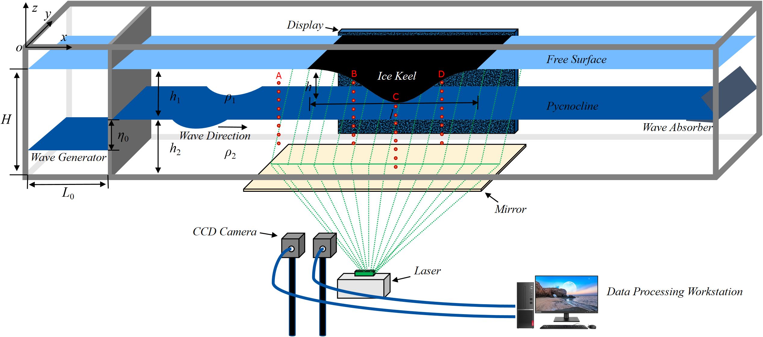
Figure 1 A schematic of the experimental setup.
Density-stratified fluids were prepared by the “two-tube” method (Fang and Du, 2005). Figure 2 shows the results of a typical stratified environment, where the total water depth was = 0.5 m; the thickness and density of the upper and lower layers were = 0.15 m, = 1003 kg/m3 and = 0.35 m, = 1019 kg/m3, respectively. The density of the contact region between two liquids is naturally continuously distributed. The vertical coordinate was the water depth, and the horizontal coordinate was the distribution of density and the Brunt-Vaisala (B-V) frequency . The B-V frequency is mathematically represented as , where is the acceleration of gravity; ρ(z) represents a vertical change in density. As shown in Figure 2, due to the mixing of two fluids in the contact area, there was a pycnocline with a thickness of ~7 cm, and the maximum B-V frequency was located near the middle of the pycnocline. The pycnocline structure thus formed was similar to the strong pycnocline structures typical of polar seas.
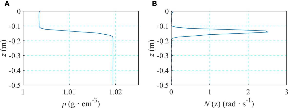
Figure 2 Distribution of density and Brunt-Vaisala (B-V) frequency in the stratified envorinment, (A): Density distribution, (B): B-V frequency distribution.
According to the known observation-based morphological characteristics of typical ice keels (Petty et al., 2016), we selected the Gaussian function to describe ice keels. Typical ice keels are known to have horizontal and vertical scales spread over hundreds and tens of meters, respectively (Strub-Klein and Sudom, 2012). The maximum slope of an ice keel is considered as its absolute slope (Debernard, 2003), which ranges from 0.17 to 0.78 for most ice keels (Wadhams and Toberg, 2012). In this experiment, with the consideration of scaled model, a Gauss ice keel made of smooth wood with length = 1.5 m, height = 0.15 m, and slope = 0.29 was selected as the experimental model. When the ice keel was placed in the flume, the upper surface coincided with the free water surface; the cartesian coordinates of the middle position along the upper edge were 5.00 m, 0 m. The width of the ice keel was equal to the inner wall of the flume, leaving no gap between the ice keel and the side wall of the flume.
To measure the evolution of ISWs, conductivity probe arrays were arranged at four positions [A ( = 4.19 m), B ( = 4.74 m), C ( = 5.00 m), and D ( = 5.25 m)] in the regions where ice keels were placed (Figure 1). Eight probes were arranged 0.02 m apart vertically at each position. The vertical position of the probe arrays could be adjusted appropriately according to the different layers during the experiment, thus ensuring that the density disturbance could be measured fully. The probes at position A were used to measure the initial ISWs, and the probes at positions B, C, and D were used to measure the evolution of ISWs under the ice keel.
The density field of the analysis regions was measured using Schlieren technology. The experimental device for this purpose consisted of a background plate, an image recorder, and data processing software. The background plate used here comprised a 2 m × 1.5 m display; a blue speckle pattern was chosen as the background image. The image recorder comprised a charge-coupled device (CCD) camera with a spatial resolution of 2592 × 2048 pixels and a capture rate of 25 frames-per-second. Processing the images by solving the Poisson equation to obtain a two-dimensional refractive index distribution. The Gladstone-Dale relation was then used to derive density field data.
The PIV method was used to measure the structure of the flow field in our regions of interest. The system comprised a laser generator, an image recorder, a data processing workstation, etc. During the experiment, the laser generator illuminated particles from a position below the transparent flume. The image recorder contained the same CCD camera as the Schlieren technology; here, two time-synchronized cameras with overlapping fields of view were used. The images were processed using the cross-correlation function calculation method of a two-dimensional fast Fourier transformation, and the initial velocity vector distribution was corrected to obtain the velocity vector.
Dimensionless parameters were introduced in the experiment:
Where is amplitude of ISW (m); is the total water depth (m); is wave speed of ISW (m/s); is the acceleration of gravity (m/s2); is the thickness of the upper layer (m), and is the thickness of the lower layer (m).
To accurately simulate the evolution of ISWs in polar seas, the stratified environment was used to denote the early observations of polar seas (Padman and Dillon, 1991; Fer et al., 2010; Kozlov et al., 2014); for this purpose, the total water depth was 0.5 m. Three types of stratified environments were set up: = 1/4, = 3/7, = 2/3. In this experiment, the step length in the wave-making region was kept constant at 0.35 m, and ISWs of different amplitudes were generated by changing the step depth. Ten experiments were conducted in each group. Table 1 shows the settings and specific parameters for these experiments.

Table 1 Experimental settings and parameters.
Figure 3 shows the visualization of the interaction between ISW and ice keel when = 3/7. The image was obtained by a high-speed camera in front of the flume. The red liquid in the middle layer depicts the pycnocline, with the upper and lower layers being the freshwater and saltwater, respectively (Figure 3). Figure 3A shows the initial state, where the vertical position of the pycnocline overlaps with the bottom of the ice keel. In Figures 3B, C, Due to the blocking action of the ice keel, the pycnocline begins to thicken near the bottom of the ice keel. At the back slope, the thickened pycnocline collapses, forming a clockwise vortex structure that alters the smooth waveform of the incident ISW (Figures 3D, E). The structure of the vortex continues to strengthen, a swell similar to the flipping characteristics related to the Kelvin Helmholtz instability (Fructus et al., 2009) appears near the back slope (Figures 3F, G). Subsequently, the structure of the vortex gradually dissipates, causing the flow to transform into turbulence and an intensified mixing of the fluid. At the same time, a portion of the fluid near the back slope is squeezed into the front slope, inducing great horizontal transport (Figures 3I, J).
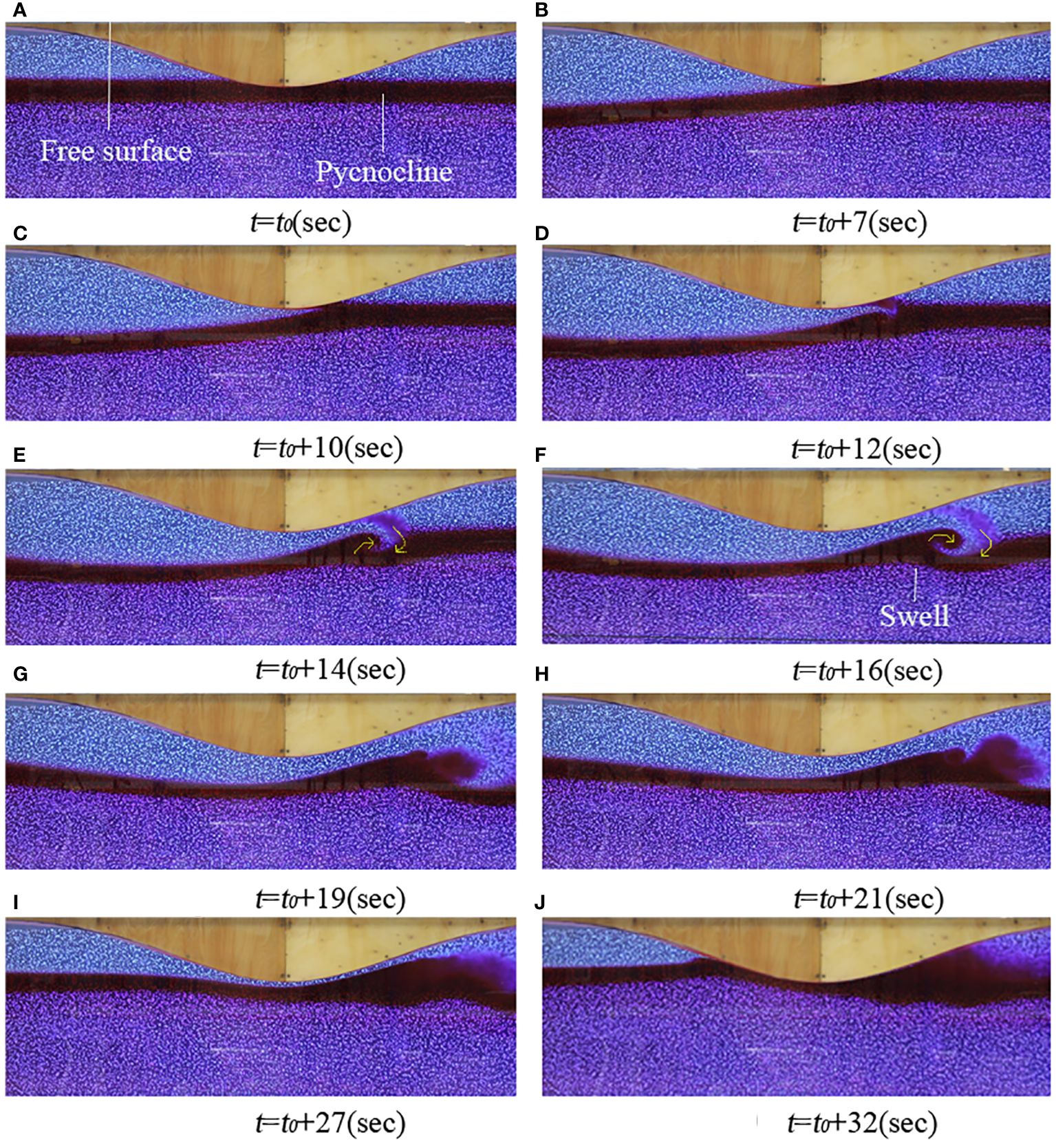
Figure 3 Visualization of the evolution of ISW beneath the ice keel, (A): Stationary state, (B–D): Reaching the back slope with the windward side of wave, (E, F): Generating vortex, (G–J): Vortex shedding and fluid mixing.
Based on the visualization results of the evolution of ISWs, the states of ISWs at the front slope, bottom, and back slope of the ice keel were analyzed. They were classified as stability, instability, and breaking by severity, as shown in Table 2. The results indicate that the states of ISWs are closely related to the amplitude of the incident wave, stratified environment, and position of ice keel.
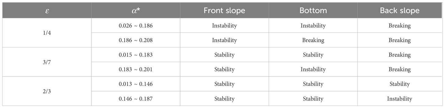
Table 2 The states of ISWs on the front slope, bottom, and back slope of the ice keel.
The variation of the waveform during the propagation of ISW was obtained using probe arrays at positions A, B, C, and D. Figure 4 shows typical waveform changes, when the stratified environment = 3/7 and the incident wave amplitude was 0.158. Figure 4A shows the initial waveform. A comparison of Figures 4A, B suggests that upon the propagation of the ISW to the front slope (position B), the waveform becomes lower and narrower due to the blocking action of the ice keel. At the same time, the wave amplitude increases. At the bottom of the ice keel (position C), the waveform of the obstructed ISW is lifted, the trough becomes very wide, and the amplitude decreases, which is consistent with the results of Carr et al. (2019). When the ISW reaches the back slope (position D), the windward side of the waveform steepens, almost perpendicular to the level, and the leeward side slows down, this is because the interaction between the ISW and the ice keel is most pronounced at the back slope. In addition, the ISW breaks free from the obstruction of the ice keel, which intensifies the mixing of the surrounding fluid, causing the trough to become extremely narrow.
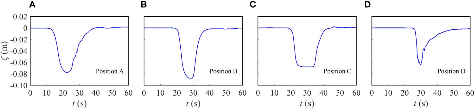
Figure 4 The variation in waveform at different positions, (A): Position A, (B): Position B, (C): Position C, (D): Position D.
Figure 5 shows the characteristics of the variation in the amplitude of the ISW beneath the ice keel. The amplitude of the ISW increases for three types of stratified environments at position B. Among them, when the stratified environment = 1/4, the increase in amplitude is the largest, reaching 11%, followed by increases in amplitude when = 3/7 and = 2/3. The main reason for the increase in wave amplitude is the nonlinear enhancement caused by the ice keel. At position C, the wave amplitude begins to decrease for the three types of stratified environments, and the intensity of the wave decreases sequentially in the order, = 1/4, = 3/7, and = 2/3, with a maximum reduction of 30% when = 1/4. The main reason for the decrease in wave amplitude is the breaking of the unstable ISW at the back slope of the ice keel. The wave amplitude remains unchanged from position C to D, with only a slight increase when = 1/4. In addition, the variation pattern is consistent for different incident wave amplitudes.
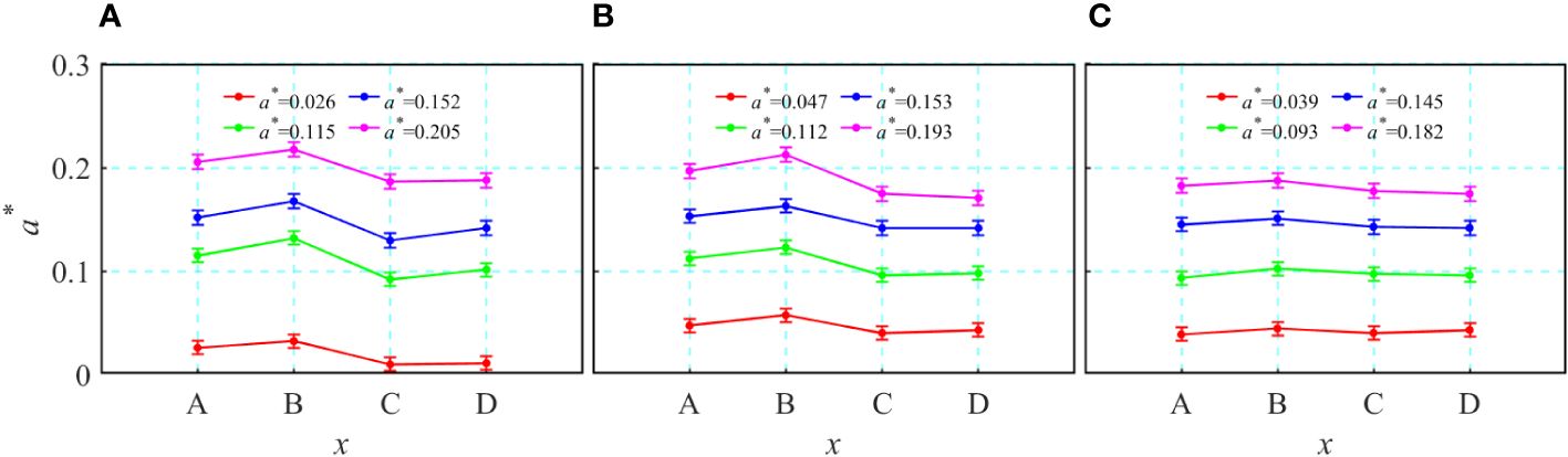
Figure 5 The variation in the wave amplitude at different positions when, (A) = 1/4, (B) = 3/7, (C) = 2/3.
In summary, the overall trend of the change in wave amplitude from position A to D in the three types of stratified environments is consistent, i.e., they all increase at first, followed by a decrease, and finally, they become stable. The reason for the change in wave amplitude is the change of nonlinear.
Figure 6 shows the characteristics of the variation in wave speed during the evolution of ISW beneath the ice keel. The ISW is obstructed by the ice keel from position A to B, and thus, its speed decreases in all three types of stratified environments. When the stratified environment =1/4, the degree of wave speed attenuation is the largest, followed by =3/7 and =2/3. At position C, when =1/4, the wave speed continues to decrease, with a maximum reduction of 38%; when =3/7, the wave speed decreases slightly; and for =2/3, the wave speed remains almost unchanged. Subsequently, the ISW reaches position D, where it breaks free from the obstruction of the ice keel. For =1/4 and =3/7, the wave speed increases significantly, but for =2/3, there are only small disturbances within a range of 5%. In addition, the incident wave amplitude has little effect on the variation of wave speed.

Figure 6 The variation in wave speed at different positions when, (A) = 1/4, (B) = 3/7, (C) = 2/3.
The above characteristics indicate that at the front slope of the ice keel, the speed of the ISW will be suppressed, while at the back slope, the speed of the ISW will be enhanced. This is due to the fact the total depth changes during the propagation of ISW.
Figure 7 shows the typical velocity and vorticity fields of ISWs for different stratified environments. According to Figure 7A, B, the blocking action of the ice keel accelerates the flow velocity in the upper fluid, casing the shear action stronger. The positive vorticity develops within a certain range near the ice keel. At the bottom of the ice keel, the Venturi effect can happen where the ice keel is high, resulting in an increase horizontal velocity of the upper fluid. At the back slope, the horizontal velocity shear continuously increases, inducing clockwise vortices. In addition, the regions of alternating with strong positive and negative vorticities are noted, indicating the occurrence of fluid mixing (Figure 7C). As the ISW propagates, the intensity and range of the clockwise vortex is enhanced, causing strong mixing of the surrounding fluid; the flow field near the ice keel becomes chaotic with a series of positive and negative phase vortices, and the mixing regions are enlarged (Figure 7D).
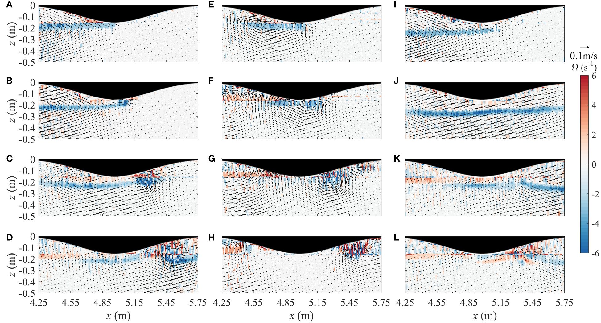
Figure 7 Velocity and vorticity fields variation of the ISW for different stratified environments, = 3/7: (A–D); = 1/4: (E–H); = 2/3: (I–L).
According to Figure 7E, due to the stronger blocking action of the ice keel, the ISW flow field forms a large vortex at the front slope, and there is only a small positive vorticity near surface of the front slope. Subsequently, the wave is truncated near the bottom of the ice keel (Figure 7F). One part of the ISW is blocked by the ice keel and is reflected, evolving into a strip of positive vorticity at the front slope. The other part continues to propagate forward along the surface of the back slope, forming a clockwise vortex that is accompanied by strong shear action (Figure 7G). Furthermore, the ISW causes a strong mixing at the back slope (Figure 7H).
Figure 7I shows that when the windward side of the wave is near the front slope, the flow field is less affected and shows a strip of negative vorticity. Subsequently, the banded negative vorticity is affected by the ice keel and causes an uplift in the valley region (Figure 7J). When the ISW passes through the back slope, the leeward side of the wave is lifted and collides with the ice keel, causing the surrounding fluid to mix, generating positive and negative vorticities (Figure 7L).
The range of the regions analyzed in this study is (m), (m). Based on experimental data on the density and flow fields of the simulated ISW, an equation to calculate the energy of two-dimensional ISW derived under non-hydrostatic approximation conditions is used (Moum et al., 2007a, b; Lamb and Nguyen, 2009). The kinetic energy density of an ISW is mathematically written as Formula 1:
Where is the constant density under the Boussinesq approximation; , represent the horizontal and vertical velocities of fluid particles, respectively. The expression for potential energy density is written as Formula 2:
Where is the vertical displacement of the isodensity line; is the flow field density when the ISW passes through; is the density of the background field without disturbance, and is the gravitational acceleration. The energy of ISW is calculated from Formulas 3–5:
Figure 8 shows the energy variation of ISW, when = 3/7, = 1/4, = 2/3. The vertical axis was , where is the energy of the ISW during propagation, and is the total energy of the incident ISW. The horizontal axis is , indicating the relative position of the ice keel. Figure 8A shows that the total, kinetic, and potential energies of the ISW remain almost unchanged during propagation if the ice keel is absent; in this situation, the kinetic energy accounted for ~52%, and potential energy accounted for ~48% of the total energy. The energy dissipation during propagation is within 4%, which is consistent with the conclusion of Chen et al. (2007).
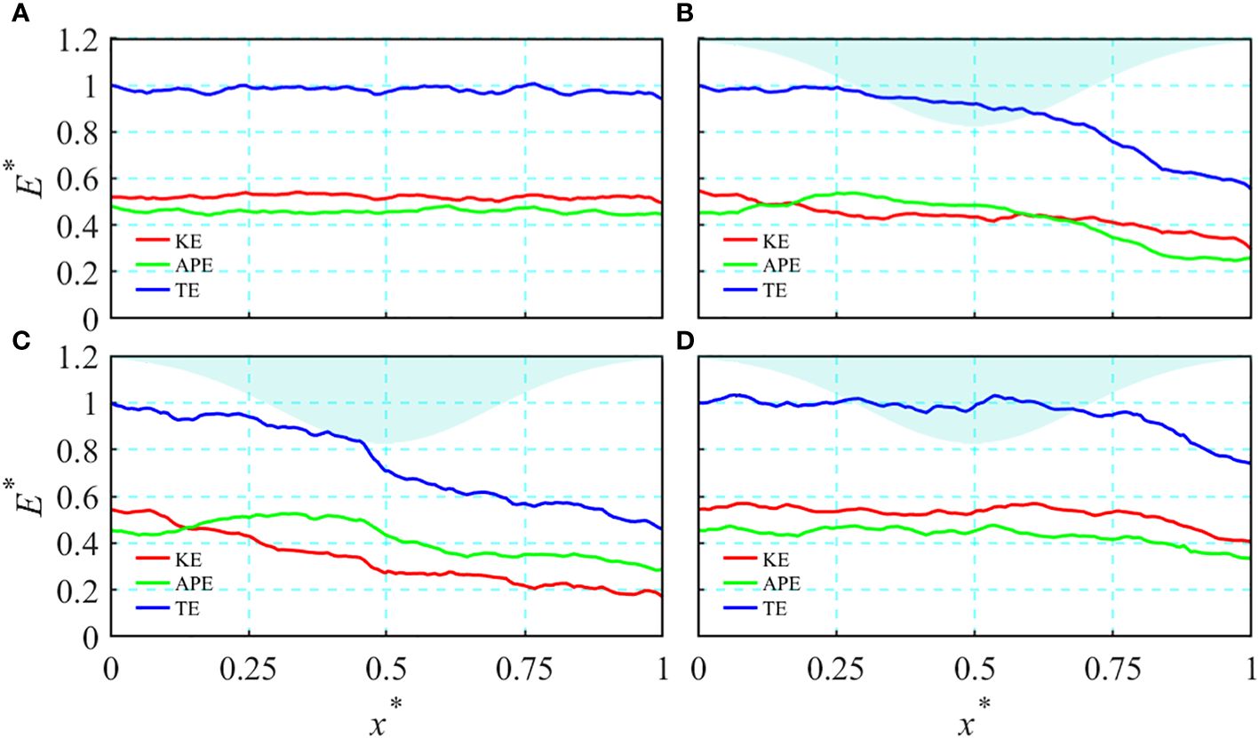
Figure 8 Energy variation of the ISW for the case, where = 3/7, = 1/4 and = 2/3, (A) = 3/7, without ice keel, (B) = 3/7, with ice keel, (C) = 1/4, with ice keel, (D) = 2/3, with ice keel.
Figures 8B–D show that the variation patterns of total, kinetic, and potential energies of the ISW are consistent for the three types of stratified environments; additionally, the maximum energy dissipation regions are located at the back slope. due to the fact that energy dissipation is mainly in the form of reflection and friction at the front slope, while it is the breaking of the ISW itself at the back slope, The differences across the stratified environments are reflected majorly in three aspects: the location at which the energy undergoes rapid dissipation, the magnitude of energy dissipation, and the occurrence of energy internal conversion. When = 1/4, energy begins to dissipate rapidly at the front slope, the total energy dissipation is ~55%, while for = 3/7 and = 2/3, the positions of rapid dissipation are sequentially located later in the flume, the total energy dissipation is ~40 and ~25% respectively. In addition, when = 1/4, = 3/7, a conversion of kinetic to potential energy is noted, while for = 2/3, no such conversion occurs. The main reason for these differences is the location and intensity of the interaction between the ISW and the ice keel in different stratified environments.
To further investigate the influence of the ice keel on the energy of ISW, the energy loss rate is calculated; it is defined as Formula 6:
Where represents the total energy of the ISW when it enters the analysis regions, and represents the total energy of the ISW when it leaves the analysis regions. In addition, by analyzing the loss of total energy from the ISW in the absence of the ice keel, it could be concluded that the energy loss rate is less than 5%. Therefore, 5% is considered to be the allowable error in calculating the energy loss rate.
Figure 9 shows the energy loss rate of the ISW for different stratified environments and incident dimensionless amplitudes . The reasons for the loss of energy from the ISW include the internal energy generated by the direct interaction between the ISW and the ice keel due to friction, and the internal energy generated by the breaking and mixing of the ISW beneath the ice keel. When = 3/7 and the ISW amplitude is small, it has greater direct contact with the ice keel, resulting in greater energy loss, as the amplitude of the ISW increases before the turning point, its direct contact with the ice keel decreases, and so does the loss of energy. However, its breaking and mixing increases after the turning point, and the energy loss increases as well. When = 1/4, the interaction between the ISW and the ice keel is intense, resulting in maximum energy loss. As the wave amplitude increases, the interaction weakens, and the energy loss decreases. When = 2/3, the interaction between the ISW and the ice keel is weak, and energy loss is minimal. As the amplitude of the ISW increases, the interaction is also enhanced, resulting in a slight increase in energy loss.
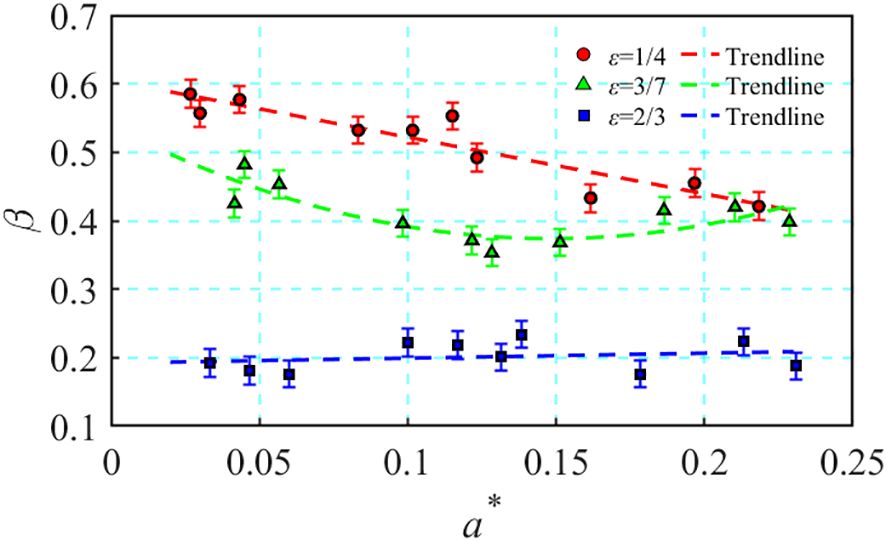
Figure 9 The rate of energy loss from the ISW.
Using a large stratified flume, laboratory experiments were conducted to study the evolution of ISWs beneath an ice keel. The evolution characteristics of ISWs were analyzed in detail to make the following conclusions:
ISW was obstructed by the ice keel, causing an increase in the thickness of the pycnocline. Subsequently, the thickened pycnocline collapsed, forming a clockwise vortex structure. This vortex structure continued to strengthen, which caused breaking and internal surging of ISW. The flow underwent strong mixing and transformed into turbulence.
Throughout the evolution of ISW, the waveform will widen or narrow with the different positions of the ISW. In addition, its wave amplitude initially increased at the front slope, then decreased at the back slope, and eventually stabilized. On the contrary, the wave speed first decreased at the front slope and increased at the back slope. Therefore, it was inferred that the stratified environment and wave amplitude influence the specific location and intensity of the evolution of ISWs.
The interaction between ISW and the ice keel enhanced the shear action and vorticity magnitude of the flow field, thereby inducing the generation of a lager vortex. The vortex formed had an unstable structure for a propagating ISW, resulting in a region of both positive and negative vorticity. This was accompanied by strong fluid mixing. The location and intensity of the formation of vortices during the evolution of the flow and vorticity fields were closely associated with the stratified environment and the amplitude of ISW.
The energy of ISW underwent internal conversion mainly at the front slope, while energy dissipation occurred largely at the back slope. The reasons for the energy dissipation of ISW included its direct physical interaction with the ice keel due to friction, and the breaking and mixing of ISW beneath the ice keel. The magnitude of energy dissipation of ISW was related to the stratified environment and its amplitude.
The raw data supporting the conclusions of this article will be made available by the authors, without undue reservation.
GW: Conceptualization, Methodology, Project administration, Software, Supervision, Writing – original draft. HD: Data curation, Formal analysis, Investigation, Resources, Validation, Writing – review & editing. JF: Data curation, Formal analysis, Validation, Writing – review & editing. SW: Data curation, Writing – review & editing. PX: Software, Visualization, Writing – review & editing. HG: Formal analysis, Writing – review & editing. JX: Data curation, Writing – review & editing. ZG: Writing – review & editing.
The author(s) declare financial support was received for the research, authorship, and/or publication of this article. This work was supported by the National Natural Science Foundation of China (Grant Nos. 11902352) and the science and technology innovation Program of Hunan Province(2023RC3005). The National Natural Science Foundation of China (Grant Nos. 42192552).
We appreciate all members for their efforts in the process of the experience in this study, and we would like to acknowledge the referees for helpful comments.
The authors declare that the research was conducted in the absence of any commercial or financial relationships that could be construed as a potential conflict of interest.
All claims expressed in this article are solely those of the authors and do not necessarily represent those of their affiliated organizations, or those of the publisher, the editors and the reviewers. Any product that may be evaluated in this article, or claim that may be made by its manufacturer, is not guaranteed or endorsed by the publisher.
Alford M. H., Peacock T., MacKinnon J. A., Nash J. D., Buijsman M. C., Centurioni L. R., et al. (2015). The formation and fate of internal waves in the South China Sea. Nature 521, 65–69. doi: 10.1038/nature14399
Bai X., Lamb K. G., Liu Z., Hu J. (2023). Intermittent generation of internal solitary-like waves on the northern shelf of the south China sea. Geophys. Res. Lett. 50, e2022GL102502. doi: 10.1029/2022GL102502
Bai X., Li X., Lamb K. G., Hu J. (2017). Internal solitary wave reflection near Dongsha Atoll, the South China Sea. J. Geophys. Res. 122, 7978–7991. doi: 10.1002/2017JC012880
Bourgault D., Janes D. C., Galbraith P. S. (2011). Observations of a large-amplitude internal wave train and its reflection off a steep slope. J. Phys. Oceanogr. 41, 586–600. doi: 10.1175/2010JPO4464.1
Carr M., Sutherland P., Haase A., Evers K., Fer I., Jensen A., et al. (2019). Laboratory experiments on internal solitary waves in ice-covered waters. Geophys. Res. Lett. 46, 12230–12238. doi: 10.1029/2019GL084710
Chen C., Hsu J., Chen H., Kuo C., Cheng M. (2007). Laboratory observations on internal solitary wave evolution on steep and inverse uniform slopes. Ocean Eng. 34, 157–170. doi: 10.1016/j.oceaneng.2005.11.019
Cole S. T., Timmermans M. L., Toole J. M., Krishfield R. A., Thwaites F. T. (2014). Ekman veering, internal waves, and turbulence observed under Arctic Sea ice. J. Phys. Oceanogr. 44, 1306–1328. doi: 10.1175/JPO-D-12-0191.1
Debernard J. (2003). Modeling the drift of ridged sea ice: A view from below. J. Geophys. Res. 108, 1–16. doi: 10.1029/2002JC001504
Du H., Wang S., Wei G., Peng P., Xuan P., Xu J. (2023). Experimental investigation of the evolution and energy transmission of a type-a internal solitary wave packet over a gentle slope. Ocean Eng. 287, 115765. doi: 10.1016/j.oceaneng.2023.115765
Fang X., Du T. (2005). Fundamentals of Oceanic Internal Waves and Internal Waves in the China Seas (Qingdao: Ocean University of China Press).
Fer I., Bosse A., Dugstad J. (2020b). Norwegian Atlantic slope current along the Lofoten Escarpment. Ocean Sci. 16, 685–701. doi: 10.5194/os-16-685-2020
Fer I., Koenig Z., Kozlov I. E., Ostrowski M., Rippeth T., Padman L., et al. (2020a). Tidally forced lee waves drive turbulent mixing along the Arctic Ocean margins. Geophys. Res. Lett. 47, e2020GL088083. doi: 10.1029/2020GL088083
Fer I., Skogseth R., Geyer F. (2010). Internal waves and mixing in the marginal ice zone near the yermak plateau. J. Phys. Oceanogr. 40, 1613–1630. doi: 10.1175/2010JPO4371.1
Filatov N. N., Zdorovennov R. E., Terzhevik A., Hutter K. (2011). Nonlinear internal waves in a large lake. Dokl. Earth Sci. 441, 1715–1718. doi: 10.1134/S1028334X11120130
Fructus D., Carr M., Grue J., Jensen A., Davies P. A. (2009). Shear induced breaking of large amplitude internal solitary waves. J. Fluid Mech. 620, 1–29. doi: 10.1017/S0022112008004898
Hartharn-Evans S. G., Carr M., Stastna M. (2024). Interactions between internal solitary waves and sea ice. J. Geophys. Res. 129, e2023JC020175. doi: 10.1029/2023JC020175
He X., Chen X., Li Q., Xu T., Meng J. (2023). Numerical simulations and an updated parameterization of the breaking internal solitary wave over the continental shelf. J. Geophys. Res. 128, 1–15. doi: 10.1029/2023JC019975
Helfrich K. R., Melville W. K. (2006). Long nonlinear internal waves. Annu. Rev. Fluid Mech. 38, 395–425. doi: 10.1146/annurev.fluid.38.050304.092129
Jackson C. (2007). Internal wave detection using the Moderate Resolution Imaging Spectroradiometer (MODIS). J. Geophys. Res. 112, C11012. doi: 10.1029/2007JC004220
Jia Y., Gong Y., Zhang Z., Yuan C., Zheng P. (2024). Three-dimensional numerical simulations of oblique internal solitary wave-wave interactions in the South China Sea. Front. Mar. Sci. 10. doi: 10.3389/fmars.2023.1292078
Kao T. W., Pan P. S., Renouard D. (1985). Internal sol tons on the Pycnocline: generation propagation, and shoaling and breaking over a slope. J. Fluid Mech. 195, 19–53. doi: 10.1017/S0022112085003081
Klymak J. M., Legg S., Alford M. H., Buijsman M., Pinkel R., Nash J. D. (2012). The direct breaking of internal waves at steep topography. Oceanogr 25, 150–159. doi: 10.5670/oceanog.2012.50
Kozlov I. E., Romanenkov D., Zimin A., Bertrand C. (2014). SAR observing large-scale nonlinear internal waves in the White Sea. Remote Sens. Environ. 147, 99–107. doi: 10.1016/j.rse.2014.02.017
Kozlov I. E., Zubkova E. V., Kudryavstev V. N. (2017). Internal solitary waves in the Laptev Sea: First results of space-borne SAR observations. IEEE Geosci. Remote S. 14, 2047–2051. doi: 10.1109/LGRS.2017.2749681
Lamb K. G. (2014). Internal wave breaking and dissipation mechanisms on the continental slope/shelf. Annu. Rev. Fluid Mech. 46, 231–254. doi: 10.1146/annurev-fluid-011212-140701
Lamb K. G., Nguyen V. T. (2009). Calculating energy flux in internal solitary waves with an application to reflectance. J. Phys. Oceanogr. 39, 559–580. doi: 10.1175/2008JPO3882.1
Levine M. D., Paulson C. A., Morison J. H. (1985). Internal waves in the Arctic Ocean: Comparison with lower-latitude observations. J. Phys. Oceanogr. 15, 800–809. doi: 10.1175/1520-0485(1985)015<0800:IWITAO>2.0.CO;2
Marchenko A. V., Morozov E. G., Muzylev S. V., Shestov A. S. (2010). Interaction of short internal waves with the ice cover in an Arctic fjord. Oceanology 50, 18–27. doi: 10.1134/S0001437010010029
McPhee M. G., Kantha L. H. (1989). Generation of internal waves by sea ice. J. Geophys. Res. 94, 3287–3302. doi: 10.1029/JC094iC03p03287
Moum J. N., Farmer D. M., Smyth W. D., Smyth W. D., Armi L. (2007a). Dissipative losses in non-linear internal waves propagating across the continental shelf. J. Phys. Oceanogr. 37, 1989–1995. doi: 10.1175/JPO3091.1
Moum J. N., Klymak J. M., Nash J. D., Perlin A., Smyth W. D. (2007b). Energy transport by nonlinear internal waves. J. Phys. Oceanogr. 37, 1968–1988. doi: 10.1175/JPO3094.1
Muench R. D., LeBlond P. H., Hachmesiter L. E. (1983). On some possible interactions between internal waves and sea ice in the marginal ice zone. J. Geophys. Res. 88, 2819–2816. doi: 10.1029/JC088iC05p02819
Nakayama K., Iwata R., Shintani T. (2021). Effect of pycnocline thickness on internal solitary wave breaking over a slope. Ocean Eng. 230, 108884. doi: 10.1016/j.oceaneng.2021.108884
Orr M. H., Mignerey P. C. (2003). Nonlinear internal waves in the South China Sea: observation of the conversion of depression internal waves to elevation internal waves. J. Geophys. Res. 108, 3064. doi: 10.1029/2001JC001163
Osborne A. R., Burch T. L. (1980). Internal solitons in the andaman sea. Science 208, 451–460. doi: 10.1126/science.208.4443.451
Padman L., Dillon T. M. (1991). Turbulent mixing near Yermak Plateau during the coordinated eastern Arctic experiment. J. Geophys. Res. 96, 4769–4782. doi: 10.1029/90JC02260
Petty A. A., Tsamados M. C., Kurtz N. T., Farrell S., Newman T., Harbeck J., et al. (2016). Characterizing Arctic Sea ice topography using high-resolution Ice Bridge data. Cryosphere. 10, 1161–1179. doi: 10.5194/tc-10-1161-2016
Pinkel R. (2005). Near-inertial wave propagation in the Western arctic. J. Phys. Oceanogr. 35, 645–665. doi: 10.1175/JPO2715.1
Rainville L., Woodgate R. A. (2009). Observations of internal wave generation in the seasonally ice-free Arctic. Geophys. Res. Lett. 36 (23). doi: 10.1029/2009GL041291
Rippeth T. P., Vlasenko V., Stashchuk N., Scannell B. D., Mattias J. A., Lincoln J. B., et al. (2017). Tidal conversion and mixing poleward of the critical latitude (an arctic case study). Geophys. Res. Lett. 44, 12349–12357. doi: 10.1002/2017GL075310
Robertson R. (2001). Internal tides and baroclinicity in the Southern Weddell sea: 1. Model description. J. Geophys. Res. 106, 27001–27016. doi: 10.1029/2000JC000475
Skyllingstad E. D., Paulson C. A., Pegau W. S., McPhee M. G., Stanton T. P. (2003). Effects of keels on ice bottom turbulence exchange. J. Geophys. Res. 108, 3372. doi: 10.1029/2002JC001488
Strub-Klein L., Sudom D. (2012). A comprehensive analysis of the morphology of first-year sea ice ridges. Cold Reg. Sci. Technol. 82, 94–109. doi: 10.1016/j.coldregions.2012.05.014
Tian Z. C., Huang J. J., Song L., Zhang M. W., Jia Y. G., Yue J. H. (2024b). The interaction between internal solitary waves and submarine canyons. J. Mar. Environ. Eng. 11, 129–139. doi: 10.32908/JMEE.v11.2024050101
Tian Z. C., Huang J. J., Xiang J. M., Zhang S. T. (2024a). Suspension and transportation of sediments in submarine canyon induced by internal solitary waves. Phys. Fluids 36, 022112. doi: 10.1063/5.0191791
Tian Z. C., Liu C., Jia Y. G., Song L., Zhang M. W. (2023). Submarine trenches and wave-wave interactions enhance the sediment resuspension induced by internal solitary waves. J. Ocean U. China. 22, 983–992. doi: 10.1007/s11802-023-5384-0
Vlasenko V., Hutter K. (2002). Numerical experiments on the breaking of solitary internal waves over a slope–shelf topography. J. Phys. Oceanogr. 32, 1779–1793. doi: 10.1175/1520-0485(2002)032<1779:NEOTBO>2.0.CO;2
Wadhams P., Toberg N. (2012). Changing characteristics of arctic pressure ridges. Polar Sci. 6, 71–77. doi: 10.1016/j.polar.2012.03.002
Xie J., Fang W., He Y., Chen Z., Liu G., Gong Y., et al. (2021). Variation of internal solitary wave propagation induced by the typical oceanic circulation patterns in the northern south China sea deep basin. Geophys. Res. Lett. 48, e2021GL093969. doi: 10.1029/2021GL093969
Xu Z., Yin B., Hou Y., Fan Z., Liu A. (2010). A Study of internal solitary waves observed on the continental shelf in the northwestern South China Sea. Acta Oceanol Sin. 29, 18–25. doi: 10.1007/s13131-010-0033-z
Zachariah R. H., Robert L. F. (2005). Internal-wave energy fluxes on the New Jersey shelf. J. Phys. Oceanogr. 35, 3–12. doi: 10.1175/JPO-2662.1
Zhang P., Li Q., Xu Z., Yin B. (2022b). Internal solitary wave generation by the tidal flows beneath ice keel in the Arctic Ocean. J. Oceanol. Limn. 40, 831–845. doi: 10.1007/s00343-021-1052-7
Zhang P., Xu Z., Li Q., You J., Yin B., Robertson R., et al. (2022a). Numerical simulations of internal solitary wave evolution beneath an ice keel. J. Geophys. Res. 127, e2020JC017068. doi: 10.1029/2020JC017068
Keywords: internal solitary waves, ice keel model, wave element, shear flow field, energy dissipation
Citation: Wang G, Du H, Fei J, Wang S, Xuan P, Guo H, Xu J and Gu Z (2024) Experimental study of internal solitary wave evolution beneath an ice keel model. Front. Mar. Sci. 11:1401646. doi: 10.3389/fmars.2024.1401646
Received: 15 March 2024; Accepted: 20 May 2024;
Published: 03 June 2024.
Edited by:
Donald B. Olson, University of Miami, United StatesReviewed by:
Yan Li, University of Bergen, NorwayCopyright © 2024 Wang, Du, Fei, Wang, Xuan, Guo, Xu and Gu. This is an open-access article distributed under the terms of the Creative Commons Attribution License (CC BY). The use, distribution or reproduction in other forums is permitted, provided the original author(s) and the copyright owner(s) are credited and that the original publication in this journal is cited, in accordance with accepted academic practice. No use, distribution or reproduction is permitted which does not comply with these terms.
*Correspondence: Hui Du, ZHVodWkxN0BudWR0LmVkdS5jbg==
Disclaimer: All claims expressed in this article are solely those of the authors and do not necessarily represent those of their affiliated organizations, or those of the publisher, the editors and the reviewers. Any product that may be evaluated in this article or claim that may be made by its manufacturer is not guaranteed or endorsed by the publisher.
Research integrity at Frontiers
Learn more about the work of our research integrity team to safeguard the quality of each article we publish.