Ocean data assimilation focusing on integral quantities characterizing observation profiles

An observation operator in data assimilation was formalized based on the signatures extracted from the integral quantities contained within observed vertical profiles in the ocean. A four-dimensional variational global ocean data assimilation system, founded on this observation operator, was developed and utilized to conduct preliminary data assimilation experiments over a ten-year assimilation window, comparing the proposed method, namely profile-by-profile matching, with the traditional method, namely point-by-point matching. The proposed method not only demonstrated a point-by-point skill comparable to the traditional method but also provided superior analysis fields in terms of profile shapes on the temperature-salinity plane. This is an indication of a well-balanced analysis field, in contrast to the traditional method, which can produce extremely poor relative errors for certain metrics. Additionally, signatures were shown to successfully represent properties of the water column, such as steric height, and serve as an effective new diagnostic tool. The top-down, or macro–micro, viewpoint in this method is fundamental to the extent that it can offer an alternative view of how we comprehend ocean observations, holding significant implications for the advancement of data assimilation.

1 Introduction

When integrating an ocean general circulation model (OGCM) under an atmospheric forcing from atmospheric reanalysis product, the state of the model ocean can deviate from observed ocean due to inevitable biases in both the model and the forcing (e.g., Lee et al., 2005; Fu et al., 2023). Therefore, the accuracy of ocean state estimations and predictions critically depends on the effective assimilation of observational data into numerical models (e.g., Marotzke and Wunsch, 1993; Stammer et al., 2002; Chang et al., 2023).

In traditional ocean data assimilation systems, observed quantities such as temperature and salinity are compared with model outputs at specific spatial points (e.g., Derber and Rosati, 1989; Malanotte-Rizzoli, 1996). The fundamental concept of this approach is the point-by-point comparison of state variables with their observed counterparts, a principle that underlies many existing data assimilation frameworks (e.g., Kalnay, 2003; Law et al., 2015).

However, when data are obtained as vertical profiles, simply focusing on temperature and salinity at each depth separately may not fully capture the information conveyed by the profile shape. The comparability of water temperature and salinity at each level can be compromised by the heaving of isopycnal surfaces (e.g., Oke and Sakov, 2008). Moreover, even if the temperature and salinity at each level are slightly similar between observations and the model, the two-dimensional curves formed by these parameters are not necessarily close, as traditional settings do not consider salinity as a function of temperature or vice versa (e.g., Haines, 2003; Dorfschäfer et al., 2020).

The fundamental distinction between the traditional method and the proposed method lies in the shift from point-to-point comparisons to comparisons between paths. For point comparisons, the objects compared could be vectors of salinity and temperature or those subjected to a linear transformation, such as through Empirical Orthogonal Functions or the balance operator (e.g., Fujii and Kamachi, 2003; Weaver et al., 2005). On the other hand, in the context of comparing paths, it is essential to acknowledge that paths are mathematically conceptualized as functions. For instance, a single profile could be envisaged as a function mapping a real parameter, which varies from 0 to 1, to a vector that includes pressure, salinity, and temperature components. Once a path is delineated as a function, any attribute of the path becomes a functional of that path. Within this analytical framework, the degree of similarity between two paths is evaluated based on the proximity of their functional values, which reflects the extent to which the paths are alike. To investigate paths from this functional perspective, focusing on the foundational elements within the functional space becomes imperative. These foundational elements are precisely what constitute the signature (Lyons et al., 2007).

The concept of path signatures, as proposed in rough path theory (Lyons, 1998; Lyons et al., 2007), has been effective in accurately processing the information present in sequential data, including profiles. The signature method, which reinterprets paths through iterated integrals, provides a novel perspective that captures the essence of information in trajectories efficiently. This method has been identified as having numerous potential applications (e.g., Fermanian, 2021), particularly in the field of earth sciences where it has been combined with machine learning techniques for predictive analysis e.g., Sugiura and Hosoda, 2020; Derot et al., 2024; Fujita et al., 2024). One significant aspect of the signature is that it serves as a functional basis within the space of functionals defined over a given set of paths. Here, the signature is called a “functional” because it maps a path, which is a function, to a number. Consequently, any functional within these sets can be accurately approximated with a linear combination of iterated integrals (Levin et al., 2013; Fermanian, 2021; Derot et al., 2024).

Our research presents a method that fundamentally reconsiders the assimilation of vertical profile data. By conceptualizing the observed vertical profiles as three-dimensional trajectories—pressure, salinity, and temperature—and comparing their signatures with those derived from numerical models, we introduce a novel approach, the signature method, which is a key concept in the theory of rough path. This method represents a significant shift from conventional point-by-point comparisons, offering a richer and more comprehensive analysis of the ocean’s water column structure.

The remainder of this paper is organized as follows. First, we present the concept of the signature and the theoretical background for its application to profiles. Next, we detail the setup of our data assimilation experiments. This is followed by a description of the results of the data assimilation experiments and their interpretation. Finally, we discuss the conclusions drawn from these results, as well as the challenges currently faced.

2 Theoretical background

Our aim is to improve the properties of vertical profiles, for example heat content, salt content, density, or sea surface height. More generally, these quantities can be attributed as a function of a profile, which can be formulated as a linear combination of iterated integrals in the signature of a path.

2.1 Signature

Signature $\mathcal{S}(X)$ for path $X:[0,1]\to {ℝ}^d$ is defined as follows (e.g., Lyons et al., 2007; Friz and Victoir, 2010). Order-n signature is composed of a series of iterated integrals,

$\begin{array}{ll}{\mathcal{S}}_{\le n}(X):=1+{\left({\mathcal{S}}_1^{(i_1)}(X)\right)}_{i_1=1,\cdots ,d}+\cdots +{\left({\mathcal{S}}_n^{(i_1\cdots i_n)}(X)\right)}_{i_1,\cdots ,i_n=1,\cdots ,d},& (1)\end{array}$

$\begin{array}{ll}{\mathcal{S}}_k^{(i_1\cdots i_k)}(X):=\underset{0}{\overset{1}{\int }}\underset{0}{\overset{u_k}{\int }}\cdots \underset{0}{\overset{u_2}{\int }}d{X}_{u_1}^{(i_1)}\cdots d{X}_{u_{k-1}}^{(i_{k-1})}d{X}_{u_k}^{(i_k)},& (2)\end{array}$

where $k=1,\cdots ,n$, and $i_1,\cdots ,i_k=1,\cdots ,d$. Note that superscripts $(i_1)$ and $(i_1\cdots i_k)$ do not denote any derivatives but simply assign a dimensional index, or multi-index. We also denote ${\mathcal{S}}_{\le n}(X)$ as $\mathcal{S}(X)$ or $ℐ$ for brevity.

A full (infinite-order) signature uniquely determines a path up to tree-like equivalence (Hambly and Lyons, 2010), and even a truncated (order-n) signature represents a path more effectively than the conventional pointwise coordinate (e.g., Fermanian, 2021; Fujita et al., 2024).

2.2 Vertical profile as signature

Imagine a path in a three-dimensional space $(P,S,T)$, labeled from $u=0$ to $u=1$ in descending order of altitude using the parameter u. The signature method represents the shape of this path using various degrees of iterated integrals. The first-order iterated integrals are the differences between the starting and ending points, defined as 3 dimensional vector $({ℐ}^P,{ℐ}^S,{ℐ}^T)={(P,S,T)}_{u=1}-{(P,S,T)}_{u=0}$. The second-order iterated integrals are defined as three pairs of areas observed from three viewpoints of this three-dimensional path (${ℐ}^{PT},{ℐ}^{TP};{ℐ}^{SP},{ℐ}^{PS};{ℐ}^{TS},{ℐ}^{ST}$; see Figure 1). In addition to the nonlinear aspects of the first-order iterated integrals (${ℐ}^{PP},{ℐ}^{TT},{ℐ}^{SS}$), a total of $9=3^2$ areas constitute the second-order iterated integrals. Although it is challenging to visualize the third-order iterated integrals, they are similarly defined by a total of $27=3^3$ volumes.

Figure 1

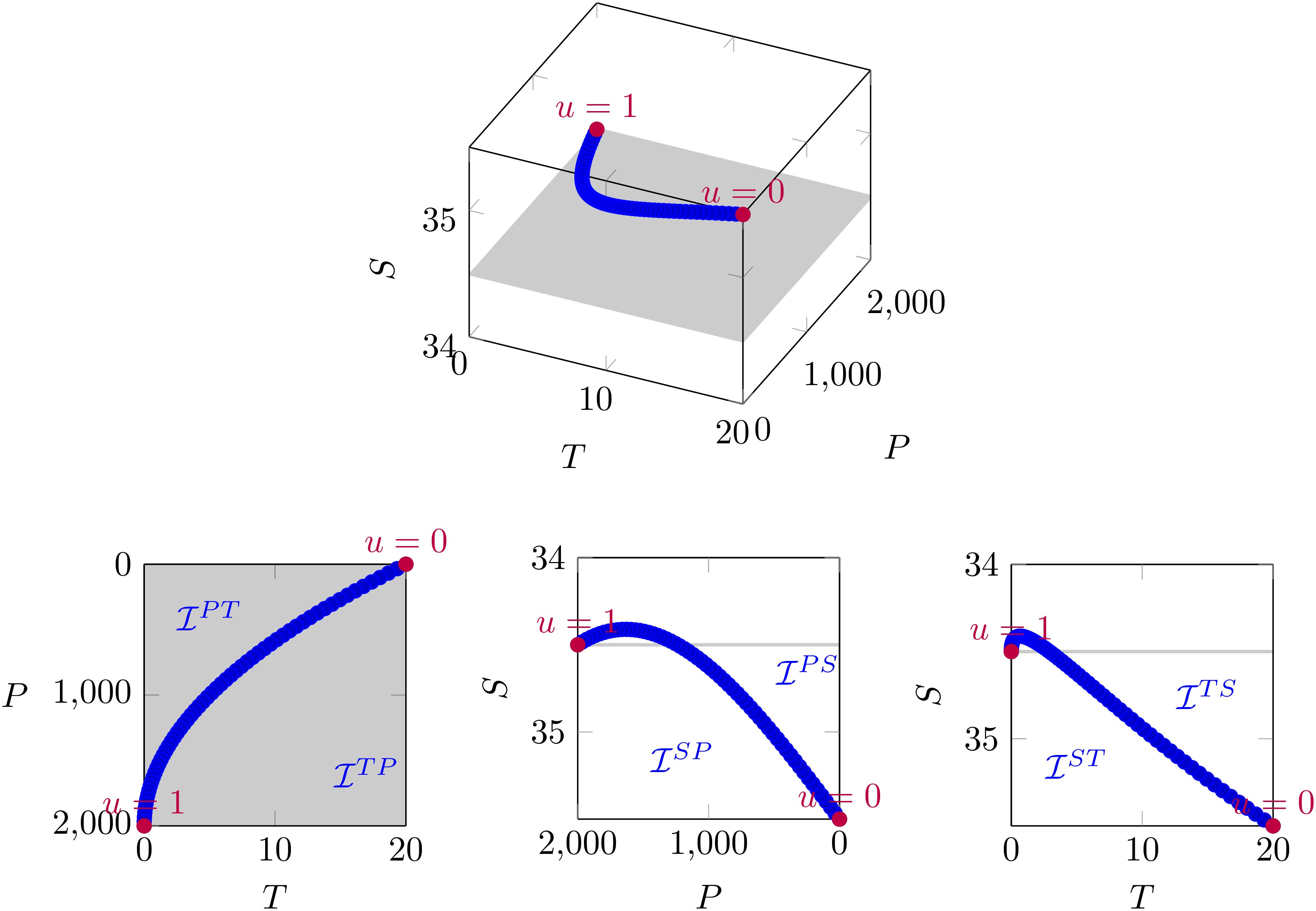
Figure 1. Grasping the shape of a profile $[0,1]\ni u\mapsto (P_u,S_u,T_u)\in {ℝ}^3$ by the second-order iterated integrals, $({ℐ}^{PT},{ℐ}^{TP},{ℐ}^{PS},{ℐ}^{SP},{ℐ}^{ST},{ℐ}^{TS})$, in signature.

In data assimilation, it is not practical to only bring specific variables closer to the observations. However, if the objective is to bring the state of the ocean closer to the state of observation, balancing the fidelity of each variable becomes important. For example, in traditional data assimilation, when assimilating observation profiles, as shown in Figure 1, a cost function is set to bring the temperature and salinity of the model at each vertical level closer to the observations. If we focus on the PS or PT planes, this policy is not likely to encounter any problems. However, considering the TS plane, the path drawn by the model profile on the plane does not necessarily approach the observation profile by assimilating only on the PS and PT planes. This is a significant drawback when the representation error of the model is significant. While incorporating spatial correlation between T and S profiles through background error covariance, as discussed by Fujii and Kamachi (2003), can help improve the adjustments on the TS plane at the level of the prior, the proposed approach emphasizes that the profile shape on the TS plane is crucial observational information, and thus is implemented as an observation operator through the signature.

As illustrated in Figure 2, the area enclosed by the temperature-salinity-profile (TS-profile) $[0,1]\ni u\mapsto (S_u,T_u)\in {ℝ}^2$ coincides with the line integral of one-form: $\omega =\frac{1}{2}((S_u-S_0)d{T}_u-(T_u-T_0)d{S}_u)$ along the profile, because of Stokes’ theorem (e.g., Spivak, 2018) (note $d\omega =d{S}_u\wedge d{T}_u$). This is sometimes called the Lévi’s stochastic area in mathematics (Lévy, 1940). This one-form vanishes if the profile is a straight line, but has some value if it is curved. By contrast, in an oceanographic context, a profile is straighter if the water is vertically well mixed, but curved if the water is stratified with multiple water masses. In other words, the area quantifies the bending of the profile in response to changes in the water mass. Thus, the area (TS-area) is a key to grasping the composition of water masses in a water column, which may be the key to understanding the T-S diagram (e.g., Mamayev, 1975; Veronis, 2021). Note that this approach shares a common philosophy with existing approaches (e.g., Cooper and Haines, 1996; Rykova, 2023) that an observation should be treated not only as values at points but also as features constrained by some conservation properties. This type of optimization can be continued for three- or higher-order iterated integrals. Mathematically, the complete set of iterated integrals from the first to higher orders is termed the signature, and it is recognized for its appropriateness and efficiency in representing the shape of a profile (e.g., Hambly and Lyons, 2010).

Figure 2

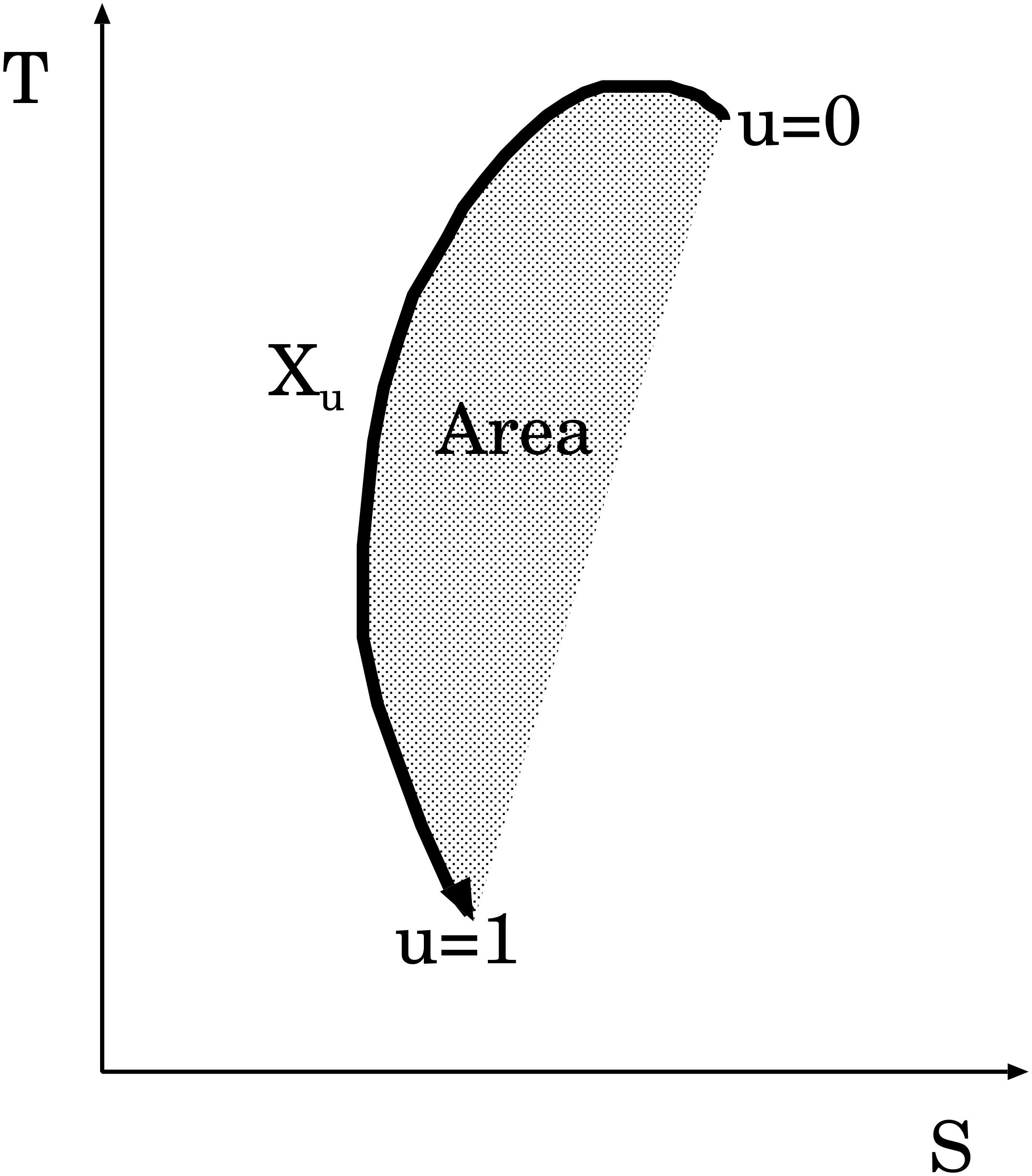
Figure 2. Example of area in temperature-salinity (T-S) diagram enclosed by profile $[0,1]\ni u\mapsto X_u=(S_u,T_u)\in {ℝ}^2$. Area is calculated as iterated integral $({ℐ}^{ST}-{ℐ}^{TS})/2:=$${\int }_{0\le u_1\le u_2\le 1}(d{S}_{u_1}d{T}_{u_2}-d{T}_{u_1}d{S}_{u_2})/2$.

2.3 Maximum mean discrepancy

Below, we will explain the comparison of the model profiles, as a probability measure, with observational profiles in our data assimilation.

Suppose that we have an inversion problem

$\begin{array}{ll}y=G(\psi )+\eta ,& (3)\end{array}$

where G is an ocean general circulation model (OGCM), ψ is the control variables (initial and boundary conditions), $G(\psi )$ is the output variables (a set of profiles), y is the observation (a set of Argo profiles), and η is the observational error.

Let ${\pi }_m$ be the restriction operator for the m-th spatiotemporal Mesh; we define the problem for mesh m as

$\begin{array}{ll}{y}_m=G_m(\psi )+{\eta }_m,& (4)\end{array}$

where $G_m:={\pi }_m\circ G$ denotes the OGCM that generates profiles in mesh m, ψ denotes the control variables (initial and boundary conditions), $G_m(\psi ):={\pi }_m\circ G(\psi )$ is the set of profiles in mesh m, y_m is the set of Argo profiles in mesh m, and η_m is the observational error for mesh m (assumed to be independent).

Now, we want to compare the model and observational (probability) measures for mesh m:

$\begin{array}{ll}\text{profile }X\in G_m(\psi )\Rightarrow X\sim P_{m,\psi },& (5)\end{array}$

$\begin{array}{ll}\text{profile}\hspace{1em}Y\in y_m\Rightarrow Y\sim Q_m.& (6)\end{array}$

These measures, $P_{m,\psi }$ and Q_m, can be approximated using the empirical measures:

$\begin{array}{ll}{\tilde{P}}_{m,\psi }=\frac{1}{\left|G_m(\psi )\right|}\sum _{X\in G_m(\psi )}{\delta }_X,& (7)\end{array}$

$\begin{array}{ll}{\tilde{Q}}_m=\frac{1}{\left|y_m\right|}\sum _{Y\in y_m}{\delta }_Y,& (8)\end{array}$

where $\left|y_m\right|$ denotes the number of observational profiles in mesh m, and ${\delta }_Y$ denotes the Dirac measure.

The distance between the two measures can be evaluated using kernel averages, which constitute maximum mean discrepancy (MMD). This approach has recently been used in estimation problems (Chérief-Abdellatif and Alquier, 2020).

When paths $X\sim P$ are embedded in the tensor space $\mathcal{T}$ of the signatures by $\mathcal{S}:X\mapsto \mathcal{S}(X)\in \mathcal{T}$, we can define the kernel mean embedding of measure P as ${\mu }_{\text{k}}(P):={\mathbb{E}}_{X\sim P}[\mathcal{S}(X)]$ (Chevyrev and Oberhauser, 2022). Subsequently, the MMD between the two measures is defined as

$\begin{array}{ll}\text{MMD}({\tilde{P}}_{m,\psi },{\tilde{Q}}_m)=\Vert {\mu }_{\text{k}}({\tilde{P}}_{m,\psi })-{\mu }_{\text{k}}({\tilde{Q}}_m){\Vert }_{\mathcal{T}},& (9)\end{array}$

where ${\Vert \Vert }_{\mathcal{T}}$ is a norm in the tensor space.

In terms of the empirical measures, Equation (9) is thus written as

$\begin{array}{ll}{\text{MMD}}^2({\tilde{P}}_{m,\psi },{\tilde{Q}}_m)={\Vert \frac{1}{\left|G_m(\psi )\right|}\sum _{X\in G_m(\psi )}\mathcal{S}(X)-\frac{1}{\left|y_m\right|}\sum _{Y\in y_m}\mathcal{S}(Y)\Vert }_{\mathcal{T}}^2.& (10)\end{array}$

This is merely a comparison of signature averages for sets of model profiles in the mesh and the observation profiles. We employed this type of observation operator in our cost function (see Methods).

3 Materials and methods

The 4D-var data assimilation system used in our experiments was constructed as follows:

3.1 Data assimilation system

3.1.1 Computation of signature

For each profile, the signature is calculated as follows: For a linear path v, represented by the vector $v\in {ℝ}^3$, the signature is computed as $\mathcal{S}(v)=e^v:={\sum }_{k=0}^n\frac{v^{\otimes k}}{k!}$, where $\otimes k$ denotes the k-times tensor product. Then, for a piecewise linear path $v_1*\dots *v_m$, made by concatenating linear paths $v_1,\cdots ,v_m$ one after the other, the signature is computed as $\mathcal{S}(v_1*\dots *v_m)=e^{v_1}\otimes \dots \otimes e^{v_m}$, because of Chen’s identity (Chen, 1958). Here, the tensor product is extended to the product in the truncated tensor algebra by $({\sum }_{k=0}^n{a}_k)\otimes ({\sum }_{k=0}^n{b}_k)={\sum }_{k=0}^n{\sum }_{j=0}^k{a}_{k-j}\otimes b_j$, where the subscript represents the order of the terms. We set the signature order to $n=4$.

3.1.2 Cost function

Our cost function is based on the comparison of mean signatures between the model and the observations made on each mesh.

We assume that vector $X_u\in {ℝ}^3$ is composed of depth, salinity, and potential temperature $(P,S,T)$. We also use the notation $X_u^{(1)}=P_u,X_u^{(2)}=S_u,X_u^{(3)}=T_u$, where $u=0$ (resp. $u=1$) corresponds to sea surface (resp. deepest measurement level $\sim 2000\text{m}$). Using the signature transform, we derive order-4 signature for each vertical profile.

In the proposed method (Sig-case), the observational cost (Sig-based cost) for each horizontal mesh m is defined as

$\begin{array}{ll}\begin{array}{c}{J}_m(\psi )=\frac{1}{2}\sum _{\tau \in T_m}\Vert \frac{1}{\left|M_{m,\tau }\right|}\sum _{X\in M_{m,\tau }}\mathcal{S}(X(\psi ))\hfill \\ {-\frac{1}{\left|N_{m,\tau }\right|}\sum _{Y\in N_{m,\tau }}\mathcal{S}(Y)\Vert }^2,\hfill \end{array}& (11)\end{array}$

where $T_m$ indicates the set of months with observed profiles for which the homogenous norm $\Vert \Vert$ is computed, $X\in M_{m,\tau }$ is the model profile in the horizontal and temporal mesh $(m,\tau )$, which is dependent on control variable ψ, and $Y\in N_{m,\tau }$ is an observational profile in mesh $(m,\tau )$. The homogenous norm assigns exponent $1/k$ to the squared sum of the k-th iterated integrals: ${\left|{\sum }_{•}|{\mathcal{S}}_k^{(•)}(X){|}^2\right|}^{1/k},$ considering nonlinear scaling with $\xi >0$ of the iterated integral: ${\mathcal{S}}_k(\xi X)={\xi }^k{\mathcal{S}}_k(X)$ (Friz and Victoir, 2010). In the reference case without signature transform (TS-case), we set the temperature-salinity-based cost (TS-based cost) as

$\begin{array}{ll}{J}_m(\psi )=\frac{1}{2}\sum _{\tau \in T_m}{\left|\frac{1}{|M_{m,\tau }|}\sum _{X\in M_{m,\tau }}X(\psi )-\frac{1}{|N_{m,\tau }|}\sum _{Y\in N_{m,\tau }}Y\right|}^2,& (12)\end{array}$

where $X\in M_{m,\tau }$ (resp. $Y\in N_{m,\tau }$) denotes model (resp. observation) temperature and salinity at gridded vertical levels in the horizontal and temporal mesh $(m,\tau )$, and $\left|\right|$ is the quadratic norm.

To enhance the representation of climatological water masses, we also applied a loose cyclicity cost term (e.g., Yu and Malanotte-Rizzoli, 1998):

$\begin{array}{ll}\begin{array}{c}{J}_{m,\text{cyc}}(\psi )=\frac{1}{2}\Vert \frac{1}{12}\sum _{\tau \in \text{first year}}\frac{1}{\left|M_{m,\tau }\right|}\sum _{X\in M_{m,\tau }}\mathcal{S}(X(\psi ))\hfill \\ {-\frac{1}{12}\sum _{\tau \in \text{last year}}\frac{1}{\left|M_{m,\tau }\right|}\sum _{X\in M_{m,\tau }}\mathcal{S}(X(\psi ))\Vert }^2,\hfill \end{array}& (13)\end{array}$

or the one without signature transform for the reference case.

In each case, the total cost is defined as

$\begin{array}{ll}\begin{array}{c}J(\psi )=\frac{1}{2}{(\psi -{\psi }_b)}^{\top }{B}^{-1}(\psi -{\psi }_b)\hfill \\ +\lambda \left(\sum _{\text{observed }m}{J}_m(\psi )+\sum _{\text{model\hspace{0.17em}}m}{J}_{m,\text{cyc}}(\psi )\right),\hfill \end{array}& (14)\end{array}$

where $B=B^{\frac{1}{2}}{B}^{\frac{\top }{2}}$ denotes the background error covariance with $B^{\frac{1}{2}}$, the composition of smoothing and scaling. In this decomposition, $B^{\frac{1}{2}}=D\circ S$, the smoothing operator S is implemented as a Laplacian smoothing (Weaver et al., 2021) with a horizontal correlation length-scale of $200km$ for the initial condition and $300km$ for fluxes. Meanwhile, the scaling operator D is implemented as a diagonal matrix based on the standard deviation of interannual variability at each point. ${\psi }_b$ is the firstguess vector, and $\lambda >0$ is a scaling factor that absorbs a possible imbalance between the background and observational terms.

By changing variable $\psi =B^{\frac{1}{2}}\varphi +{\psi }_b$, the original cost function is rewritten as that with respect to $\varphi$:

$\begin{array}{ll}\mathcal{J}(\varphi )=\frac{1}{2}{\varphi }^{\top }\varphi +\lambda \left(\sum _{\text{observed\hspace{0.17em}}m}{J}_m(B^{\frac{1}{2}}\varphi +{\psi }_b)+\sum _{\text{model\hspace{0.17em}}m}{J}_{m,\text{cyc}}(B^{\frac{1}{2}}\varphi +{\psi }_b)\right).& (15)\end{array}$

The derivation of its gradient is explained in Supplementary Material Sec. 2.

3.1.3 Gradient method

The 4D-Var data assimilation problem was solved iteratively using Nesterov’s accelerated gradient method (Nesterov, 1983). See Supplementary Material Sec. 3 for details regarding the implementation.

3.2 Experimental settings

Our data assimilation experiment aimed to compare the proposed case (Sig-case) to the signature-based cost (Equation 11) and reference case (TS-case) to TS-based cost (Equation 12). The experimental setting was as follows:

3.2.1 Ocean general circulation model

The OGCM we used is a version of the Meteorological Research Institute Community (MRI.com) models (Tsujino et al., 2010, 2011). It is equipped with a mixed-layer model (Noh and Jin Kim, 1999) and coupled with a sea ice model (Hunke and Dukowicz, 2002). The global ocean was set as the simulation domain. for 10 years ($T=120$ in Equation 11) from January 2004 to December 2013. This model was coupled with a sea ice model. It was divided into spatial meshes of resolution $1\times 0.5$ degrees and temporal meshes with monthly resolution. For example, a spatiotemporal mesh was defined in the following range: of 10N to 10.5N, 140E to 141E, February 2012.

3.2.2 Firstguess

Before data assimilation (DA), the OGCM was spun up using climatological air-sea fluxes, with nudging toward the climatological temperature and salinity fields, and then integrated from 1959 to December 31, 2003, under interannual air-sea fluxes to obtain a firstguess snapshot, which was used as the initial condition at the start of DA iteration. The air-sea fluxes used were compiled as daily means from JRA-55 atmospheric reanalysis dataset. (Kobayashi et al., 2015) These values were then linearly interpolated from 10 elements of daily-mean field: surface air temperature, 10 m wind vector (2-dimensional), scalar wind, shortwave radiation flux, longwave radiation flux, precipitation, river runoff, dew point temperature, and sea level pressure. We refer to the model state at the start of DA iteration as firstguess.

3.2.3 Control variables

Our 4D-Var is a strong constraint (Talagrand and Courtier, 1987), which has a 10-year-long assimilation window without any temporal gaps in ocean states. The control variables ψ were the initial state (of the first year) and the increments in air-sea fluxes in a 10-day span, which were linearly interpolated. Among the initial states, we updated 5 ocean state variables— temperature, salinity, horizontal velocity (2-dimensional), and sea-surface height— but not for the sea-ice and mixed-layer states.

3.2.4 Adjoint model

The adjoint OGCM was derived through automatic differentiation of the Fortran code using TAF (Giering and Kaminski, 2003). For applicability to long assimilation windows, the forward variables required for the adjoint integration were stored in scratch files as temporal mean during forward integration and then restored for adjoint integration. For the sake of stability in the sensitivity calculation (Sugiura et al., 2014), we did not use the adjoint of the sea ice model or the mixed-layer model. Regarding the signature transform, we must compute the gradient (adjoint) of the signature transform, which is also derived by applying the automatic differentiation of the Fortran code. Our implementation of the signature module is available on GitHub.

3.2.5 Assimilated data

To determine the effect of the signature method on the profile data, we assimilated only the Argo profiles (Argo, 2020) that have three elements (pressure P, salinity S, and temperature T) and vertical lengths of nearly $2000m$. The area from the southern shore of Greenland to the far north Atlantic was excluded from the observational area because of the poor representation ability of the model around there. For the comparison with the model state, the in-situ temperature was converted into potential temperature, and the pressure was converted into depth. As a simple observational error variance, $(P,S,T)$ are normalized by their typical variations, $(2000\text{m},8\mathrm{psu},20\text{K})$, before the signature transform. Additionally, after several trials, we set $\lambda ={10}^6$ in Equation 14.

4 Results

4.1 Variation of cost function

Figure 3 shows the variation in the cost function during the iterations. The signature-based cost (Equation 11) decreased almost monotonically in Sig-case because it was the minimization object but fluctuated in TS-case, converging to a higher value. TS-based cost (Equation 12) showed the opposite behavior. Naturally, the two minimization problems have distinct stationary points, leading to different estimates. Note that Sig-case also reduced TS-based costs considerably, which guarantees a certain level of compatibility with traditional TS-based cost function settings.

Figure 3

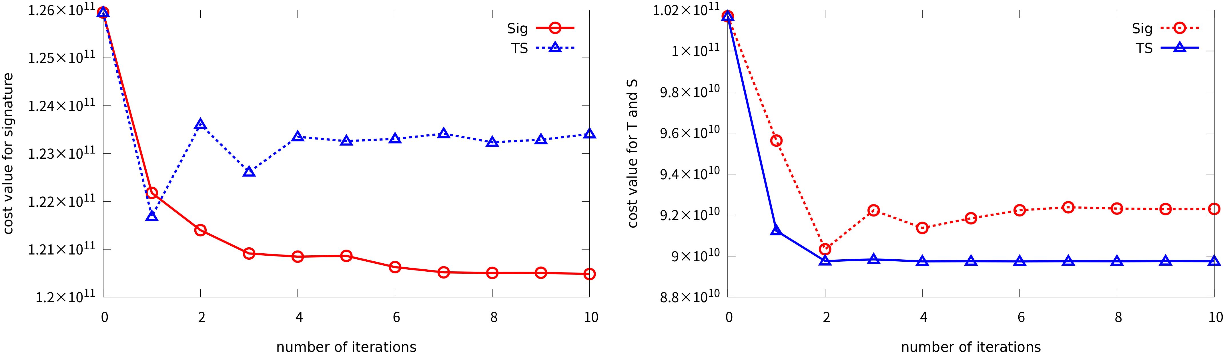
Figure 3. Variation in the cost functions in terms of signature-based cost (left) and TS-based cost (right). Sig-case is shown by red circles, TS-case by blue triangles.

To observe the breakdown of the reduction in the observational cost term, the relative error from firstguess was calculated for each iterated integral up to degree 3. The relative error ${ϵ}_I$ was defined as the root mean squared error of the estimated field against the observation across all the observed meshes, divided by that of firstguess:

$\begin{array}{ll}{ϵ}_I^2:=\frac{{\sum }_{\text{observed\hspace{0.17em}}m}{\sum }_{\tau \in T_m}{\nu }_{m,\tau ,I}^2(\psi )}{{\sum }_{\text{observed\hspace{0.17em}}m}{\sum }_{\tau \in T_m}{\nu }_{m,\tau ,I}^2({\psi }_b)},& (16)\end{array}$

where

$\begin{array}{ll}{\nu }_{m,\tau ,I}(\psi ):=\frac{1}{\left|M_m\right|}\sum _{X\in M_{m,\tau }}{\mathcal{S}}^{(I)}(X(\psi ))-\frac{1}{\left|N_m\right|}\sum _{Y\in N_{m,\tau }}{\mathcal{S}}^{(I)}(Y).& (17)\end{array}$

Figure 4 compares the relative errors for each iterated integral for Sig-case and TS-case. Iterated integrals composed only of index P showed no change because we cannot change the depth span of a profile. Iterated integrals that include both T and S generally showed a decrease in Sig-case, but some terms increased in TS-case, which is likely owing to the lack of direct observational constraints on such metrics in TS-case. For iterated integrals that did not include both T and S, the two cases exhibit a similar behavior, but TS-case was slightly better than Sig-case in general. Overall, most of the terms showed a decrease from firstguess in both cases. Although TS-case generally showed a better performance than Sig-case, it sometimes showed a significant increase from firstguess (for example, in ${ℐ}^{STT}$ or ${ℐ}^{STP}$). In summary, Sig-case showed a balanced improvement, whereas, in TS-case, the improvement was skewed and some deterioration were observed in terms of the T-S diagram.

Figure 4

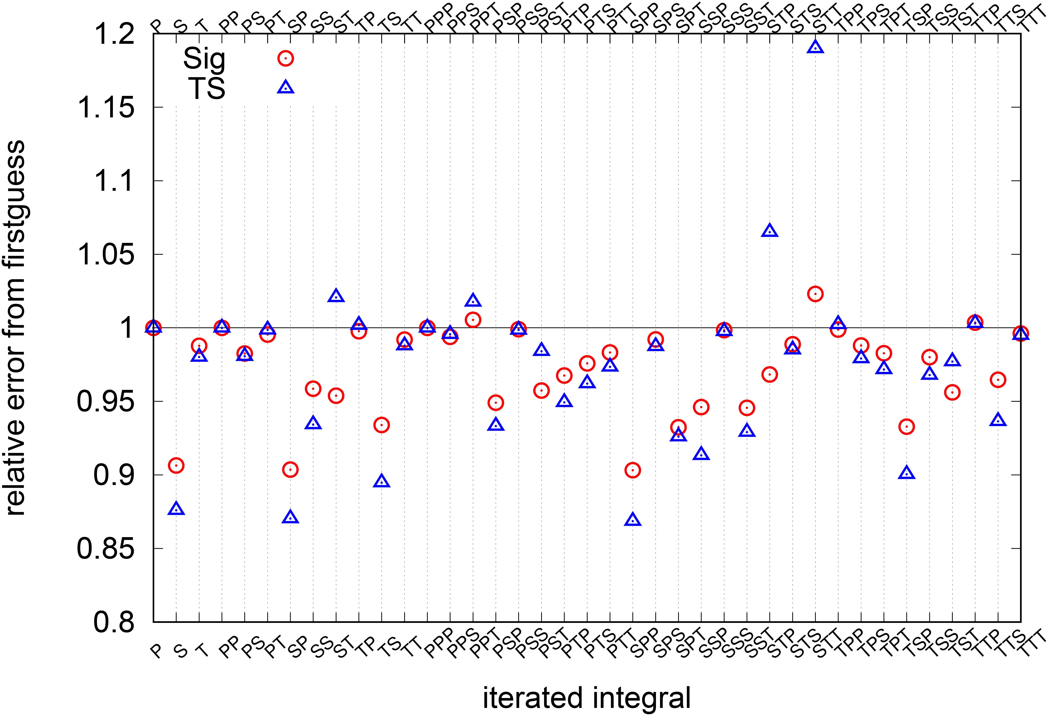
Figure 4. Relative error to firstguess for each iterated integral. Sig-case is denoted by red circles and TS-case by triangles. Horizontal axis is the index of iterated integral, for example, TS represents ${ℐ}^{TS}$.

4.2 Point-by-point performance

As evident in the right panel of Figure 3, the total pointwise errors in temperature and salinity have no significant difference between Sig-case and TS-case. To uncover the difference, we will first examine the point-by-point performance of both cases by showing the horizontal distributions of the root mean square errors (RMSEs) against observations at several vertical levels. To emphasize the differences between the two cases, we show the RMSEs relative to that of the firstguess. Figures 5 and 6 indicate the RMSEs for temperature at $200\text{m}$ and $1500\text{m}$, respectively. Both cases have relatively small RMSEs, but the contrast is more significant in the TS-case, which means that some regions show notable improvements, while others show deteriorations. For example, the temperature at $200\text{m}$ in the Kuroshio recirculation region, and the temperature at $1500\text{m}$ in the Indian Ocean, became worse than the firstguess. On the other hand, the deteriorations in the Sig-case are more suppressed than in the TS-case. Figures 7 and 8 indicate the RMSEs for salinity at $0\text{m}$ and $700\text{m}$, respectively. Again, the contrast is more significant in the TS-case. For example, the sea surface salinity in the Kuroshio recirculation region, and the salinity at $700\text{m}$ in some regions along the Antarctic Circumpolar Current, became significantly worse than the firstguess. On the other hand, the deteriorations in the Sig-case are more suppressed than in the TS-case.

Figure 5

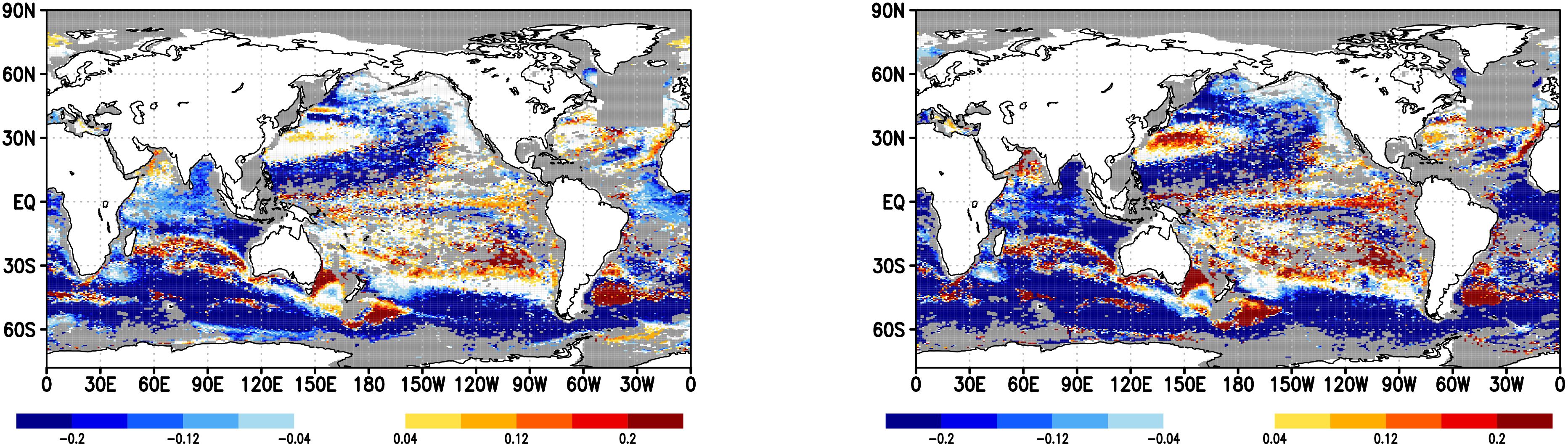
Figure 5. Change in RMSEs against observations of 200m temperature for Sig-case (left) and TS-case (right). The change is shown as the RMSE of each case minus that of the firstguess. Unit is K.

Figure 6

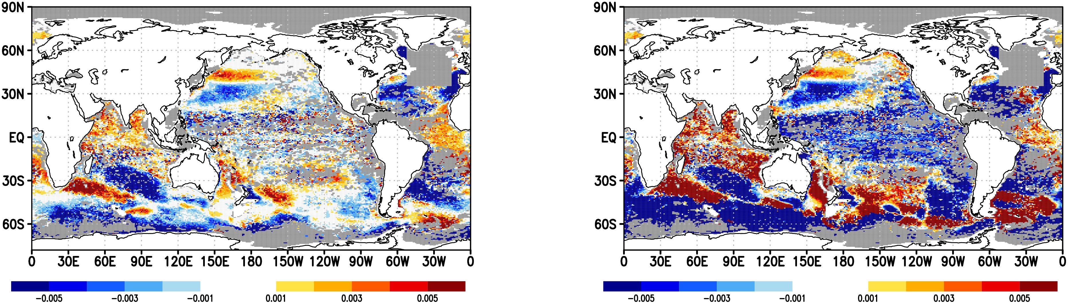
Figure 6. Change in RMSEs against observation of 1500m temperature for Sig-case (left), and TS-case (right). The change is shown as the RMSE of each case minus that of the firstguess. Unit is K.

Figure 7

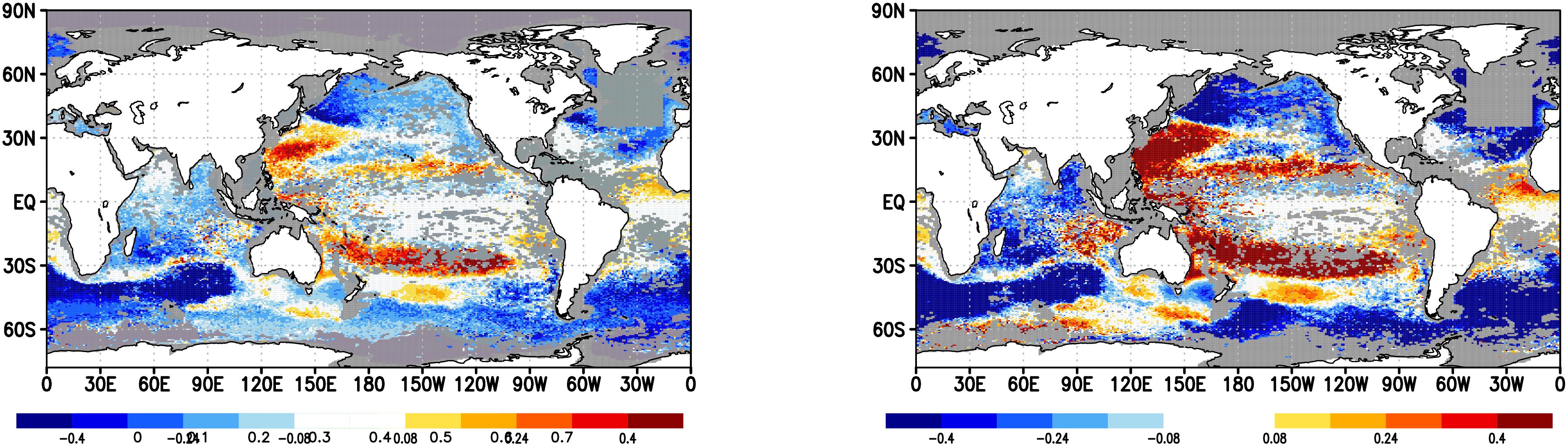
Figure 7. Change in RMSEs against observation of sea surface salinity for Sig-case (left), and TS-case (right). The change is shown as the RMSE of each case minus that of the firstguess. Unit is psu.

Figure 8

Figure 8. Change in RMSEs against observation of 700m salinity for Sig-case (left), and TS-case (right). The change is shown as the RMSE of each case minus that of the firstguess. Unit is psu.

Figures 9 and 10 present the comparison of T-S-P (TS, PT, and PS) diagrams as illustrative examples. In Figure 9B, there is no significant problem in the temperature representation, but the difference is evident in the salinity representation. The TS-case (blue in Figure 9C) shows a poor representation of surface salinity by attempting to match the salinity at each level to the observation. On the other hand, the Sig-case (red in Figure 9C) shows an accurate representation of surface salinity by aligning the first iterated integral ${\int }^{}dS$ with the observation. The structure of the salinity minimum remains unchanged from the firstguess in both cases. In Figure 10, we observe a mostly barotropic structure along the Antarctic Circumpolar Current. Improvements on the PS plane can be seen in the shallow salinity structure (Figure 10C). Both cases have surface salinity closer to the observation than the firstguess. However, the curve shape of on the TS plane looks better in Sig-case (Figure 10A).

Figure 9

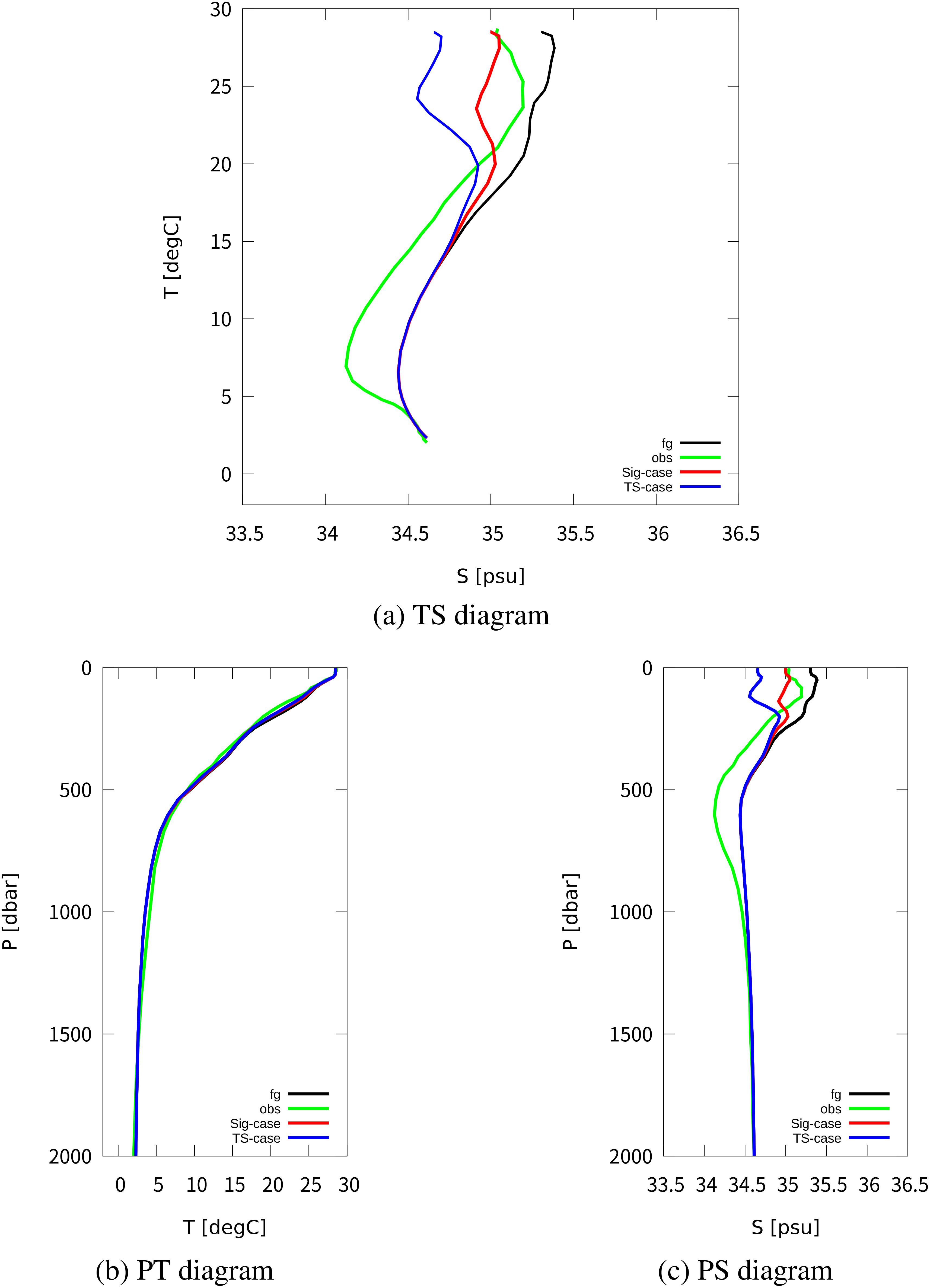
Figure 9. Comparison of T-S-P diagrams in the Kuroshio recirculation region. The temporal average values at 157 degrees east and 20 degrees north are shown for observation (green), firstguess (black), Sig-case (red), and TS-case (blue). The units are practical salinity unit (psu) for salinity, degree Celsius for temperature, and dbar for pressure. RMSEs for temperature are $0.72K$ (firstguess), $0.55K$ (Sig-case), and $0.49K$ (TS-case). RMSEs for salinity are $0.23psu$ (firstguess), $0.18psu$ (Sig-case), and $0.30psu$ (TS-case). (A) TS diagram. (B) PT diagram. (C) PS diagram.

Figure 10

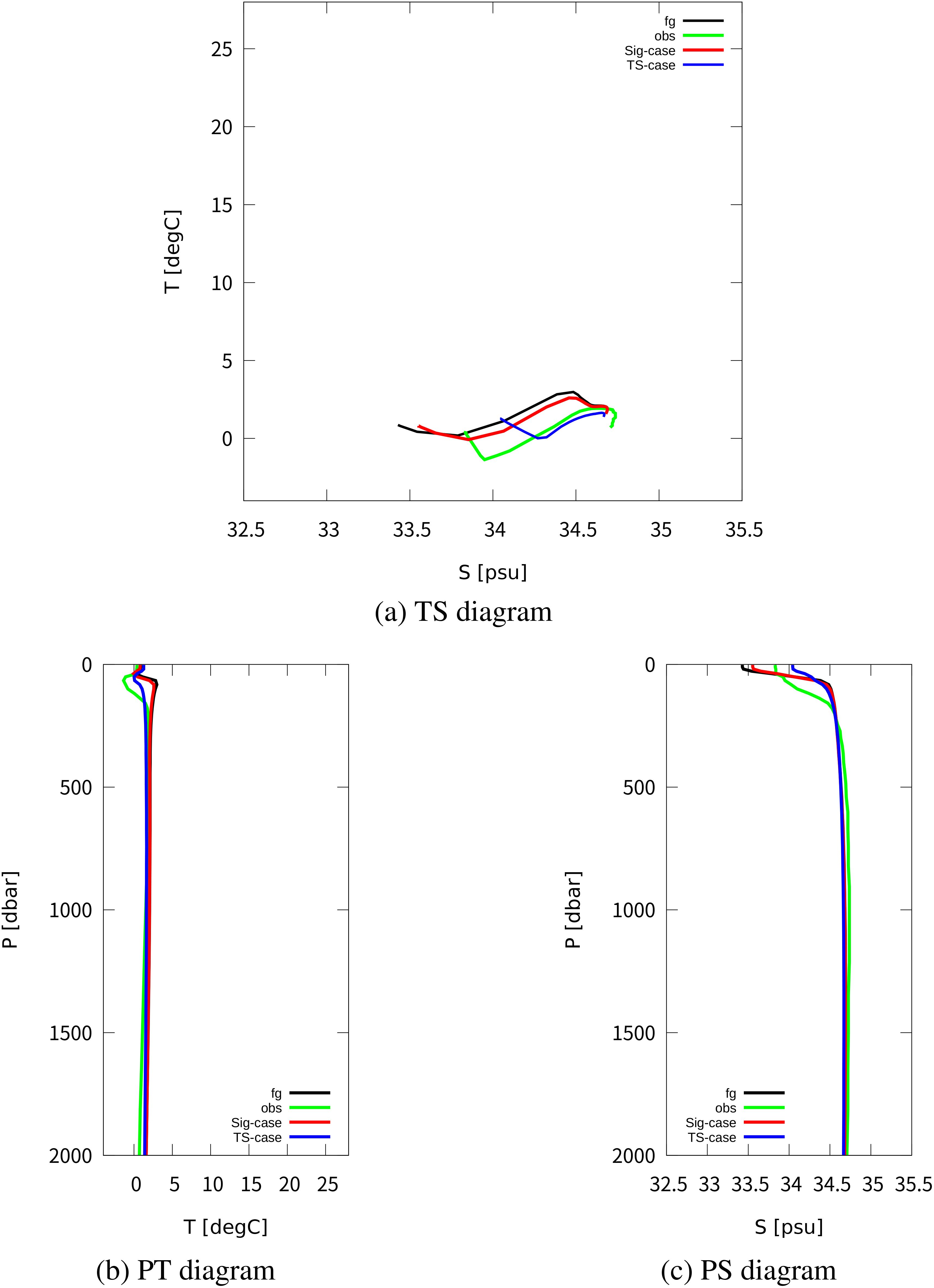
Figure 10. Comparison of T-S-P diagrams in a region along the Antarctic Circumpolar current. The temporal average values at 130 degrees east and 60 degrees south are shown for observation (green), firstguess (black), Sig-case (red), and TS-case (blue). The units are practical salinity unit (psu) for salinity, degree Celsius for temperature, and dbar for pressure. RMSEs for temperature are $1.35K$ (firstguess), $1.19K$ (Sig-case), and $0.69K$ (TS-case). RMSEs for salinity are $0.19psu$ (firstguess), $0.16psu$ (Sig-case), and $0.16psu$ (TS-case). (A) TS diagram. (B) PT diagram. (C) PS diagram.

4.3 TS-area

As shown in Figure 2 the area enclosed by TS-profile (TS-area) is important for characterizing water properties in a water column. To this end, we compared the proximity of TS-area to observations in the estimated fields. Figure 11 shows the temporal averages of TS-area $({ℐ}^{ST}-{ℐ}^{TS})/2$, in the observation, firstguess, Sig-case, and TS-case. While common shortcomings stand out in the model fields, some improvements can be observed from firstguess in Sig-case. Principally, this term indicates a salinity drop or surge in T-S diagram near the sea surface due to precipitation or evaporation (e.g., Sugiura, 2021). To observe this in detail, we derive the relative error in the model fields, which is defined as follows: Let $y_{\alpha }$ be a linear combination of iterated integrals ${\sum }_{I\in \text{Γ}}{\alpha }_I{\mathcal{S}}^{(I)}(X(\psi ))$, where ${\alpha }_I\in ℝ$ is a coefficient, and Γ is a set of multi-indices. Using ${\nu }_{m,\tau ,I}(\psi )$ in Equation 17, the relative error of $y_{\alpha }$ for each mesh, ${ϵ}_{m,\alpha }$, and overall relative error, ${ϵ}_{\alpha }$, are defined as respectively. Figure 12 shows the distribution of the relative error for TS-area (${\alpha }_{ST}=0.5,{\alpha }_{TS}=-0.5$) in the model fields. The overall relative error was 0.967 in Sig-case and 1.027 in TS-case. Both showed a similar pattern, with a noticeable decrease in errors around the Antarctic circumpolar current but an increase in errors in the subtropical circulation. Moreover, this difference was more intense in TS-case, with a more pronounced deterioration in subtropical circulation (see also Supplementary Material Sec. 4). Noting that our data assimilation is not solely for the Lévy area, the correction tendency in these two regions can be explained by the consistency of corrections with respect to iterated integral ${\int }^{}dS$ (surface salinity, or SSS) and ${\int }^{}(TdS-SdT)$ (Lévy area). Along the Antarctic circumpolar current, Figure 10A suggests that matching model SSS to observations is compatible with matching the Lévy area to observations. On the other hand, as suggested by Figure 9A, matching model SSS to observations conflicts with matching the Lévy area to observations in the subtropical regions. In TS-case, “the Lévy area” should be interpreted as salinity at the intermediate layer”.

$\begin{array}{ll}{ϵ}_{m,\alpha }^2:=\frac{{\sum }_{\tau \in T_m}{({\sum }_{I\in \Gamma }{\alpha }_I{\nu }_{m,\tau ,I}(\psi ))}^2}{{\sum }_{\tau \in T_m}{({\sum }_{I\in \Gamma }{\alpha }_I{\nu }_{m,\tau ,I}({\psi }_b))}^2},& (18)\end{array}$

$\begin{array}{ll}{ϵ}_{\alpha }^2:=\frac{{\sum }_{\text{observed\hspace{0.17em}}m}{\sum }_{\tau \in T_m}{({\sum }_{I\in \text{Γ}}{\alpha }_I{\nu }_{m,\tau ,I}(\psi ))}^2}{{\sum }_{\text{observed\hspace{0.17em}}m}{\sum }_{\tau \in T_m}{({\sum }_{I\in \text{Γ}}{\alpha }_I{\nu }_{m,\tau ,I}({\psi }_b))}^2},& (19)\end{array}$

Figure 11

Figure 11. Temporal averages of TS-area $({ℐ}^{ST}-{ℐ}^{TS})/2$, in observation (top left), firstguess (top right), Sig-case (bottom left), and TS-case (bottom right). Unit is $psu·K$.

Figure 12

Figure 12. Relative observational error of TS-area, $({ℐ}^{ST}-{ℐ}^{TS})/2$, to firstguess. Overall relative error is 0.967 for Sig-case (left) and 1.027 for TS-case (right). Blue denotes the regions of greatest improvement.

Similarly, Figure 13 shows the temporal averages of TS-volume $({ℐ}^{STT}-{ℐ}^{TST})/2$ (see Figure 14 for the meaning), in observation firstguess, Sig-case, and TS-case. In observation, this volume showed a high value around the warm water pool in the Indo-Pacific region but low value around the high evaporation areas. Such features were also observed in the model fields, but common shortcomings in terms of the shape of the high evaporation zones in the firstguess remained in both Sig-case and TS-case. Figure 15 shows the distribution of the relative error in the model fields by applying Equation 18 to ${\alpha }_{STT}=0.5,{\alpha }_{TST}=-0.5$. The error pattern is similar to the relative error for TS-area $({ℐ}^{ST}-{ℐ}^{TS})/2$ shown in Figure 12, with higher constant in TS-case. The overall value for TS-volume was 1.031 in Sig-case and 1.172 in TS-case. No overall improvement was observed in Sig-case, and deterioration was observed in TS-case.

Figure 13

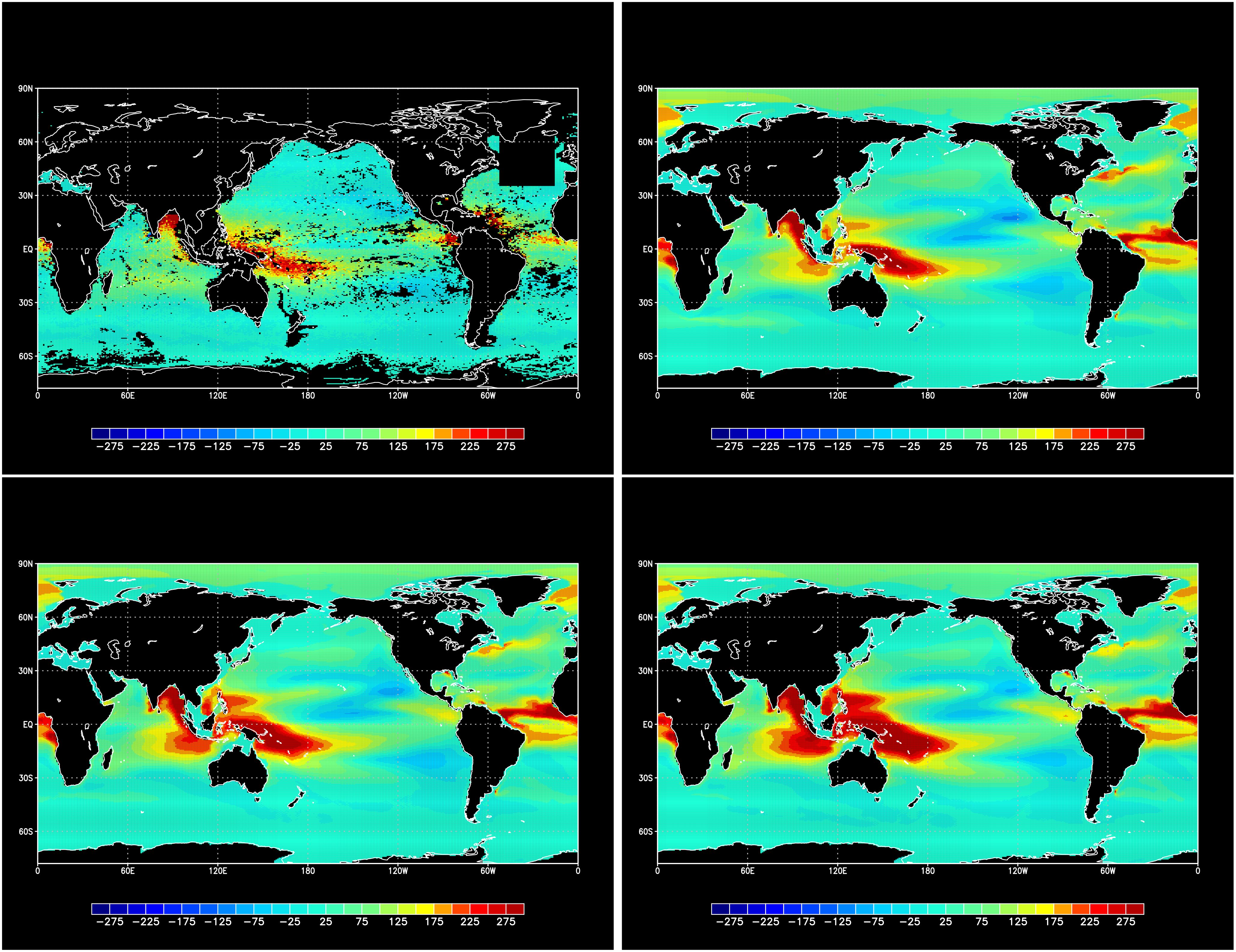
Figure 13. Temporal average of TS-volume $({ℐ}^{STT}-{ℐ}^{TST})/2$, in observation (top left), firstguess (top right), Sig-case (bottom left), and TS-case (bottom right). Unit is $psu·K^2$.

Figure 14

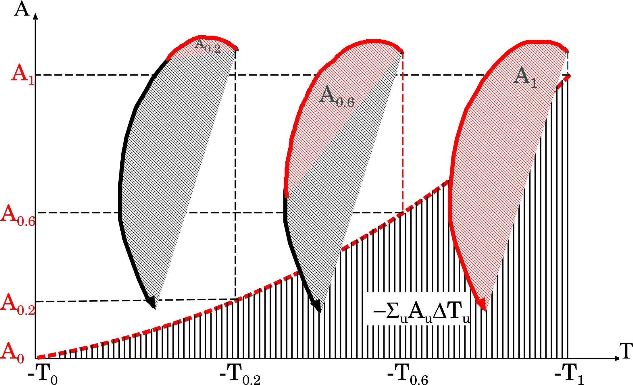
Figure 14. Example of volume in temperature-salinity (T-S) diagram enclosed by profile $[0,1]\ni u\mapsto X_u=(S_u,T_u)\in {ℝ}^2$. Volume is calculated as iterated integral $({ℐ}^{STT}-{ℐ}^{TST})/2=\underset{0}{\overset{1}{\int }}{A}_{u}d{T}_u,$ where area $A_u:={\int }_{0\le u_1\le u_2\le u}(d{S}_{u_1}d{T}_{u_2}-d{T}_{u_1}d{S}_{u_2})/2$ as in Figure 2. Typically, $u\mapsto T_u$ decreases monotonically.

Figure 15

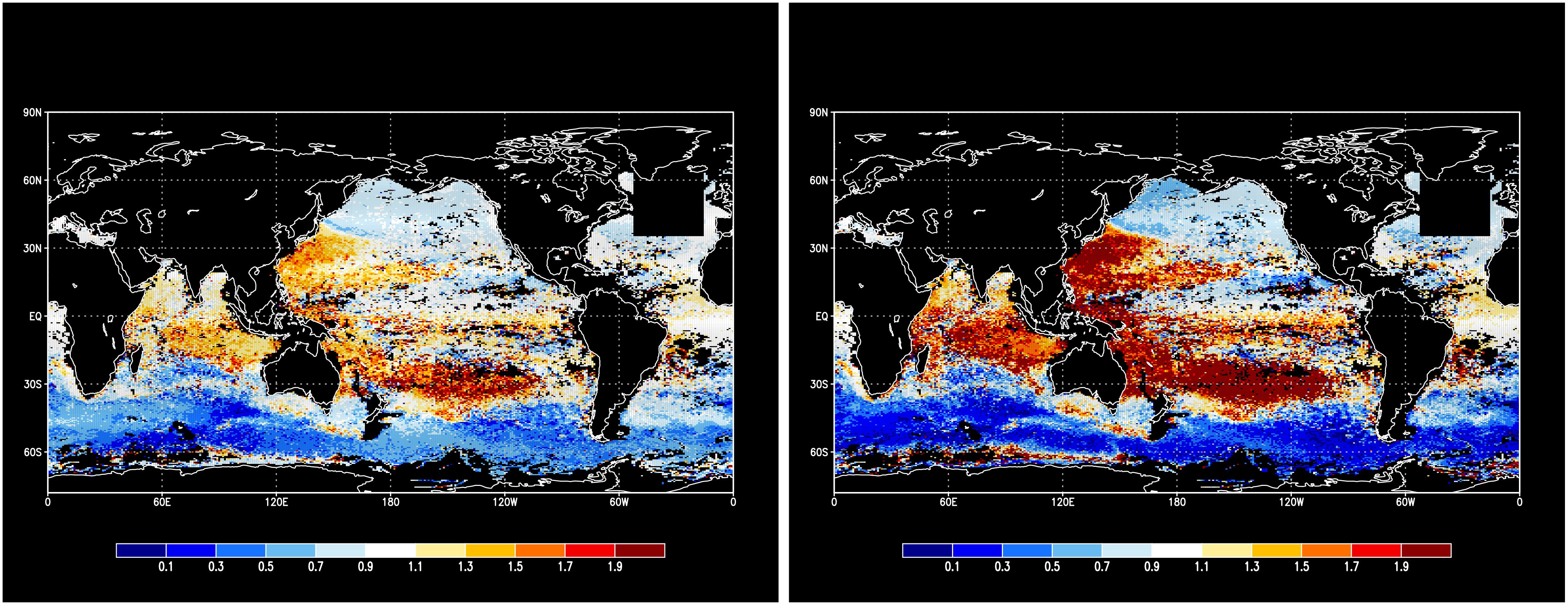
Figure 15. Relative observational error of TS-volume $({ℐ}^{STT}-{ℐ}^{TST})/2$ to firstguess. Overall relative error is 1.031 for Sig-case (left) and 1.172 for TS-case (right). Blue denotes the regions of greatest improvement.

4.4 Steric height

Owing to the universal approximation theorem (Derot et al., 2024), a nonlinear function on a set of paths can be approximated by a linear combination of the iterated integrals with any accuracy. We leverage this fact for approximating the steric height assigned to each profile.

By considering up to the second-order nonlinearity in the state equation, the steric sea level was estimated using iterated integrals for each horizontal point m as

$\begin{array}{ll}\begin{array}{c}{h}_m=-{\beta }_S{ℐ}_m^{PS}-{\beta }_T{ℐ}_m^{PT}+2{\beta }_{S^2}{ℐ}_m^{PSS}+2{\beta }_{T^2}{ℐ}_m^{PTT}\\ +{\beta }_{ST}\left({ℐ}_m^{PST}+{ℐ}_m^{PTS}\right)-{\beta }_{SP}{ℐ}_m^{PPS}-{\beta }_{TP}{ℐ}_m^{PPT}+C,\end{array}& (20)\end{array}$

where ${ℐ}_m^{•}$ denotes an averaged iterated integral for all the profiles in mesh m, and C is a constant along time. See the Supplementary Material Sec. 1 for the derivation. The coefficient values are listed in Table 1. Figure 16 shows the temporal averages of the estimated steric height minus the global mean for observation, firstguess, Sig-case, and TS-case. The firstguess assumption seems to represent the pattern of the steric anomaly to a certain extent; however, improvement is not evident in Sig-case or TS-case.

Table 1

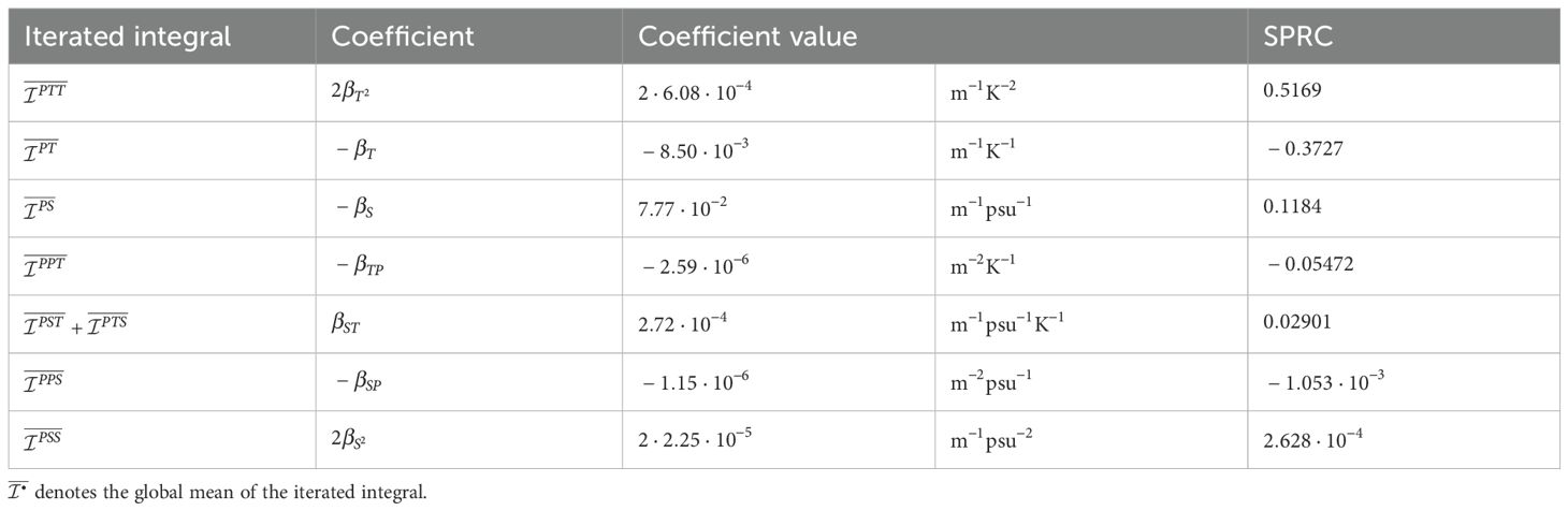
Table 1. Standard partial regression coefficients (SPRC) in the estimation of global mean steric sea level, displayed in descending order from dominant terms.

Figure 16

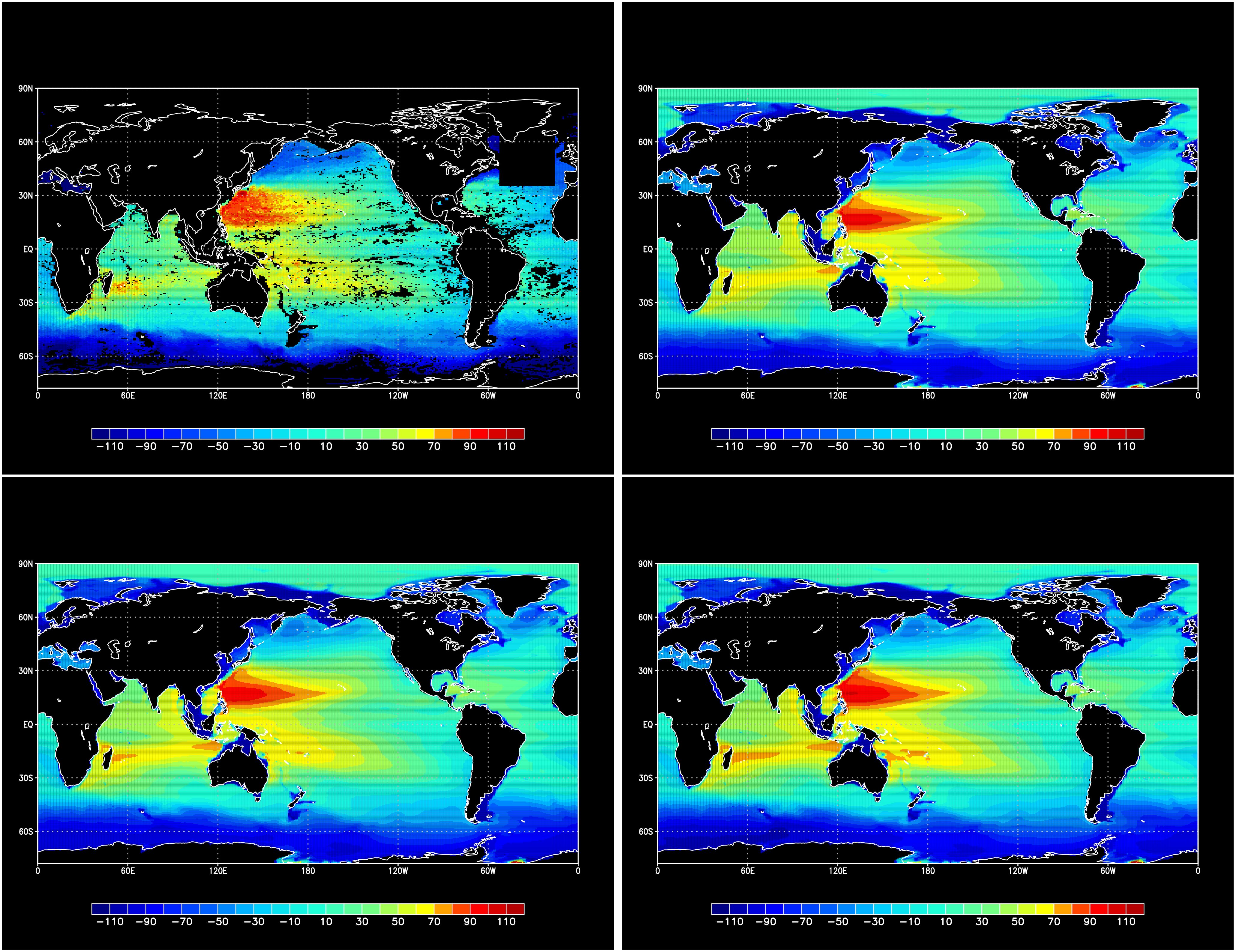
Figure 16. The temporal average in cm of steric height minus global mean, in observation (top left), firstguess (top right), Sig-case (bottom left), and TS-case (bottom right).

To determine where the improvement could be observed, we derived the relative error by applying Equation 18 to ${\alpha }_I={\beta }_I$. Figure 17 shows the distribution of the relative observational error of steric height to firstguess. There was an obvious deterioration around the Antarctic circumpolar current and subarctic circulation in both cases, but there was a slight improvement in other areas. The contrast was stronger in TS-case, resulting in a large deterioration around the Antarctic circumpolar current. The overall relative error estimated using Equation 19 was 1.000 for Sig-case and 1.013 for TS-case, which means that no overall improvement by DA was observed in Sig-case, and TS-case was slightly worse. Given that DA did not necessarily improve the agreement of steric height with observations, we do not discuss about the estimate of the global average steric height.

Figure 17

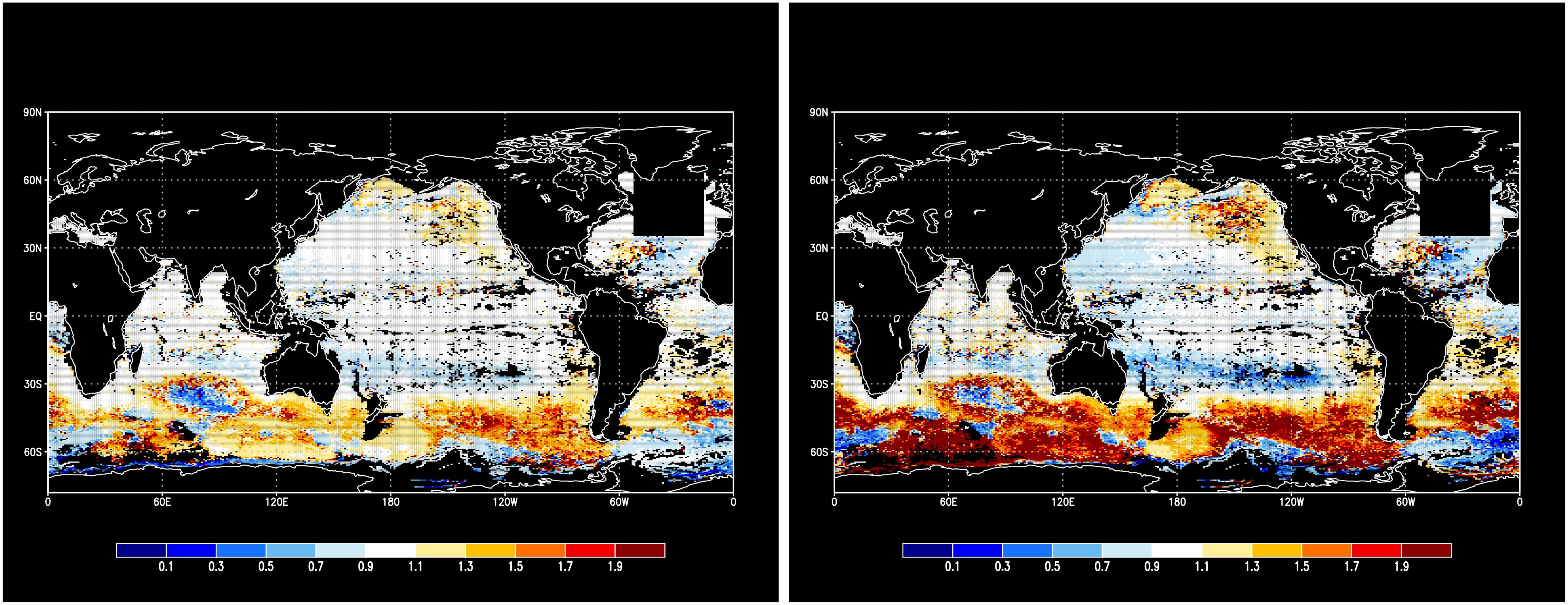
Figure 17. Relative observational error of steric height to firstguess. The overall relative error is 1.000 for Sig-case (left) and 1.013 for TS-case (right). Blue denotes the regions of greatest improvement.

The estimation Formula 20 is more informative than just for estimating steric height. For example, we can also obtain information regarding which iterated integral is dominant in the estimation of the global mean steric sea level (GMSSL). By integrating Equation 20 over the global ocean, we obtain a linear regression formula for GMSSL for each month:

$\begin{array}{ll}\begin{array}{c}\overline{h}=-{\beta }_S\overline{{ℐ}_m^{PS}}-{\beta }_T\overline{{ℐ}_m^{PT}}+2{\beta }_{S^2}\overline{{ℐ}_m^{PSS}}+2{\beta }_{T^2}\overline{{ℐ}_m^{PTT}}\\ +{\beta }_{ST}\left(\overline{{ℐ}_m^{PST}}+\overline{{ℐ}_m^{PTS}}\right)-{\beta }_{SP}\overline{{ℐ}_m^{PPS}}-{\beta }_{TP}\overline{{ℐ}_m^{PPT}}+C,\end{array}& (21)\end{array}$

where $\overline{{ℐ}^{•}}={\sum }_m{ℐ}^{•}{A}_m/A$, with ${\sum }_m$ the summation over global ocean domain, $A_m$ the area of each mesh, and $A={\sum }_m{A}_m$. Using this equation, we can compute the Standardized Partial Regression Coefficients (SPRCs) (McClendon, 2002) for a linear regression model that predicts the monthly mean GMSSLs. The SPRCs from the results of our experiment are shown in Table 1. The most dominant terms are thermosteric terms ${\beta }_{T^2}$ and ${\beta }_T$. By contrast, the contribution of the TS-cross term ${\beta }_{ST}$ was sufficiently small compared with that of the dominant terms: ${\beta }_{T^2}$, ${\beta }_T$, and ${\beta }_S.$ The dominant terms, ${\beta }_{T^2}$ and ${\beta }_T$, clearly indicate that thermosteric changes are more dominant compared to halosteric changes or the cross effects. Furthermore, the most dominant term, ${\beta }_{T^2}$, demonstrates that regions characterized by high temperature layers significantly contribute to thermosteric effects. The slightly worse overall relative error for steric sea level (1.013) to firstguess in TS-case might be attributed to the deterioration of iterated integrals ${\mathcal{I}}^{\mathcal{P}\mathcal{P}\mathcal{T}}$ and ${\mathcal{I}}^{\mathcal{P}\mathcal{S}\mathcal{T}}$ in Figure 4, at least partially.

5 Discussion

1. We developed a method to enhance ocean state estimates by comparing mean signatures of observed vertical profiles against those of model profiles within a framework of the four-dimensional variational DA. This novel approach was meticulously formulated and implemented, aiming to harness the comprehensive information embedded within vertical profile trajectories. We applied this implementation to ocean DA with a decadal assimilation window.

2. Our DA experiment demonstrated that the signature method can achieve improvements in temperature and salinity estimations that are comparable to those attained by conventional methods. This finding ensures the sanity of our implementation as a DA method.

3. Importantly, the utilization of signatures allowed for a certain level of enhancement in the representation of profile shapes on the TS plane, a critical aspect that traditional ocean DA approaches have largely overlooked. This advancement highlights the potential to properly capture the water mass and the dynamics of oceanic processes.

4. This type of cost function provides a more safety-side assessment; in other words, it will no longer be the case that only some aspects improve and other aspects become significantly worse (Refer to Figure 4).

5. Furthermore, the signature formulation can be used as an evaluation formula for various properties of the water column. For instance, steric heights could be directly assessed from iterated integrals derived during the DA experiment, showcasing the versatility of the signature method in representing various oceanographic properties.

6. The comprehensive analysis revealed that the use of a signature-based observation operator not only achieves comparable improvements in temperature and salinity fields as conventional methods but also enhances previously neglected aspects, such as profile shapes on the TS plane. This dual capability marks a significant step forward in the field of DA involving shape matching.

7. This method provides a versatile framework applicable to DA of observational profiles across various dimensions, not limited to ocean profiles. Given a multidimensional profile, it is capable of considering the shape of paths composed of any combinations of two or even more variables that have mostly been overlooked in traditional DA.

8. Furthermore, our setting of observational cost is broadly applicable in DA practices incorporating profile observations, extending its utility beyond four-dimensional variational approaches to include ensemble methods. This flexibility suggests a wide range of potential applications for the signature method in improving the accuracy and efficiency of state estimations and predictions.

By embracing the essence of oceanic phenomena through the innovative use of signatures, this study offers a promising new direction for DA techniques, potentially enhancing our understanding of oceanography by estimating the ocean states more accurately.

Finally, the limitations of the experimental settings and methods must be mentioned.

1. In the present experimental setup, the model was not well-tuned, and the representation errors were pronounced to the extent that the advantages of the proposed method could not be fully demonstrated. To clearly demonstrate the significance of using signatures, more experiments in an effective assimilation setting under appropriate tuning are needed, with comprehensive observations to be assimilated.

2. While the transformation to signatures has been modularized in Fortran, to facilitate its integration as an extension to conventional methods, a comprehensive understanding of the signature concept is crucial. For example, the independence of observation variables should be crucial for the observation operator to perform better. In our case, the iterated integrals inherently have multicollinearity. To reduce this dependency, we can make use of log-signature (e.g., Lyons et al., 2007) or apply whitening by using the observational covariance between iterated integrals.

3. Related to the covariance, implementing this approach involves using several ad hoc constants for scaling and weighting the observational data. This reliance on arbitrary parameters introduces an element of subjectivity and may affect the reproducibility and universality of the method. A more rigid formulation upon which the assimilation is set is desirable.

4. Operational forecasting models assimilate not only vertical profiles but also observations taken on the surface (e.g., Sea Surface Temperature, Sea Surface Height). To systematically incorporate surface observations, we need to extend the notion of path (1-parameter) signature to surface (2-parameter) signature. The mathematical setting for how a 2-parameter signature can be consistently defined is still an active research topic (Diehl and Schmitz, 2023; Diehl et al., 2024, and references therein). Therefore, for now, traditional treatments with point-by-point matching on the surface remain a practical solution to be used in data assimilation.

Data availability statement

The datasets presented in this study can be found in online repositories. The names of the repository/repositories and accession number(s) can be found in the article/Supplementary Material. The Fortran module used for signature transform in this study can be found in the GitHub repository https://github.com/nozomi-sugiura/signature_fortran.

Author contributions

NS: Conceptualization, Data curation, Formal analysis, Funding acquisition, Investigation, Methodology, Project administration, Resources, Software, Supervision, Validation, Visualization, Writing – original draft, Writing – review & editing. SK: Funding acquisition, Project administration, Supervision, Writing – original draft, Writing – review & editing. SO: Investigation, Validation, Writing – original draft, Writing – review & editing.

Funding

The author(s) declare financial support was received for the research, authorship, and/or publication of this article. This work was supported by the JSPS KAKENHI (Grant JP22H05207, Japan), and JST AIP Trilateral AI Research (Grant JPMJCR20G5, Japan).

Acknowledgments

The DA experiments were conducted using the Earth Simulator of the Japan Agency for Marine–Earth Science and Technology.

Conflict of interest

The authors declare that the research was conducted in the absence of any commercial or financial relationships that could be construed as a potential conflict of interest.

Publisher’s note

All claims expressed in this article are solely those of the authors and do not necessarily represent those of their affiliated organizations, or those of the publisher, the editors and the reviewers. Any product that may be evaluated in this article, or claim that may be made by its manufacturer, is not guaranteed or endorsed by the publisher.

Supplementary material

The Supplementary Material for this article can be found online at: https://www.frontiersin.org/articles/10.3389/fmars.2024.1398901/full#supplementary-material

References

Argo (2020). Argo float data and metadata from Global Data Assembly Centre (Argo GDAC) - Snapshot of Argo GDAC of December 10th 2020. doi: 10.17882/42182#79118

Crossref Full Text | Google Scholar

Chang I., Kim Y. H., Jin H., Park Y.-G., Pak G., Chang Y.-S. (2023). Impact of satellite and regional in-situ profile data assimilation on a high-resolution ocean prediction system in the northwest pacific. Front. Mar. Sci. 10. doi: 10.3389/fmars.2023.1085542

Crossref Full Text | Google Scholar

Chen K.-T. (1958). Integration of paths–A faithful representation of paths by noncommutative formal power series. Trans. Am. Math. Soc. 89, 395–407. doi: 10.2307/1993193

Crossref Full Text | Google Scholar

Chérief-Abdellatif B.-E., Alquier P. (2020). “MMD-Bayes: Robust Bayesian estimation via maximum mean discrepancy,” in Symposium on Advances in Approximate Bayesian Inference (Proceedings of Machine Learning Research). Cambridge MA: JMLR (Journal of Machine Learning Research) 1–21.

Google Scholar

Chevyrev I., Oberhauser H. (2022). Signature moments to characterize laws of stochastic processes. J. Mach. Learn. Res. 23, 7928–7969.

Google Scholar

Cooper M., Haines K. (1996). Altimetric assimilation with water property conservation. J. Geophys. Res.: Oceans 101, 1059–1077. doi: 10.1029/95JC02902

Crossref Full Text | Google Scholar

Derber J., Rosati A. (1989). A global oceanic data assimilation system. J. Phys. Oceanogr. 19, 1333–1347. doi: 10.1175/1520-0485(1989)019<1333:AGODAS>2.0.CO;2

Crossref Full Text | Google Scholar

Derot J., Sugiura N., Kim S., Kouketsu S. (2024). Improved climate time series forecasts by machine learning and statistical models coupled with signature method: A case study with el niño. Ecol. Inf. 79, 102437. doi: 10.1016/j.ecoinf.2023.102437

Crossref Full Text | Google Scholar

Diehl J., Ebrahimi-Fard K., Harang F., Tindel S. (2024). On the signature of an image. arXiv preprint arXiv:2403.00130. doi: 10.48550/arXiv.2403.00130

Crossref Full Text | Google Scholar

Diehl J., Schmitz L. (2023). Two-parameter sums signatures and corresponding quasisymmetric functions. arXiv preprint arXiv:2210.14247. doi: 10.48550/arXiv.2210.14247

Crossref Full Text | Google Scholar

Dorfschäfer G. S., Tanajura C. A. S., Costa F. B., Santana R. C. (2020). A new approach for estimating salinity in the southwest atlantic and its application in a data assimilation evaluation experiment. J. Geophys. Res.: Oceans 125, e2020JC016428. doi: 10.1029/2020JC016428.E2020JC016428

Crossref Full Text | Google Scholar

Fermanian A. (2021). Embedding and learning with signatures. Comput. Stat Data Anal. 157, 107148. doi: 10.1016/j.csda.2020.107148

Crossref Full Text | Google Scholar

Friz P. K., Victoir N. B. (2010). Multidimensional stochastic processes as rough paths: theory and applications Vol. 120 (Cambridge, England: Cambridge University Press).

Google Scholar

Fu H., Dan B., Gao Z., Wu X., Chao G., Zhang L., et al. (2023). Global ocean reanalysis cora2 and its inter comparison with a set of other reanalysis products. Front. Mar. Sci. 10. doi: 10.3389/fmars.2023.1084186

Crossref Full Text | Google Scholar

Fujii Y., Kamachi M. (2003). A reconstruction of observed profiles in the sea east of Japan using vertical coupled temperature-salinity EOF modes. J. Oceanogr. 59, 173–186. doi: 10.1023/A:1025539104750

Crossref Full Text | Google Scholar

Fujita M., Sugiura N., Kouketsu S. (2024). Prediction of atmospheric profiles with machine learning using the signature method. Geophys. Res. Lett. 51, e2023GL106403. doi: 10.1029/2023GL106403

Crossref Full Text | Google Scholar

Giering R., Kaminski T. (2003). Applying taf to generate efficient derivative code of fortran 77-95 programs. PAMM: Proc. Appl. Math. Mechan. 2, 54–57. doi: 10.1002/pamm.200310014

Crossref Full Text | Google Scholar

Haines K. (2003). “Assimilation of hydrographic data and analysis of model bias,” in Data Assimilation for the Earth System. Eds. Swinbank R., Shutyaev V., Lahoz W. A. (Springer Netherlands, Dordrecht), 309–320.

Google Scholar

Hambly B., Lyons T. (2010). Uniqueness for the signature of a path of bounded variation and the reduced path group. Ann. Math. 171 (1), 109–167. doi: 10.4007/annals

Crossref Full Text | Google Scholar

Hunke E. C., Dukowicz J. K. (2002). The elastic–viscous–plastic sea ice dynamics model in general orthogonal curvilinear coordinates on a sphere—incorporation of metric terms. Month. Weather Rev. 130, 1848–1865. doi: 10.1175/1520-0493(2002)130<1848:TEVPSI>2.0.CO;2

Crossref Full Text | Google Scholar

Kalnay E. (2003). Atmospheric modeling, data assimilation and predictability (Cambridge, England: Cambridge university press).

Google Scholar

Kobayashi S., Ota Y., Harada Y., Ebita A., Moriya M., Onoda H., et al. (2015). The JRA-55 reanalysis: General specifications and basic characteristics. J. Meteorol. Soc. Japan. Ser. II 93, 5–48. doi: 10.2151/jmsj.2015-001

Crossref Full Text | Google Scholar

Law K., Stuart A., Zygalakis K. (2015). Data Assimilation (Heidelberg, Germany: Springer).

Google Scholar

Lee S.-K., Enfield D. B., Wang C. (2005). Ocean general circulation model sensitivity experiments on the annual cycle of western hemisphere warm pool. J. Geophys. Res.: Oceans 110 (9), C09004. doi: 10.1029/2004JC002640

Crossref Full Text | Google Scholar

Levin D., Lyons T., Ni H. (2013). Learning from the past, predicting the statistics for the future, learning an evolving system. arXiv preprint arXiv:1309.0260. doi: 10.48550/arXiv.1309.0260

Crossref Full Text | Google Scholar

Lévy M. P. (1940). Le mouvement brownien plan. Am. J. Math. 62, 487–550. doi: 10.2307/2371467

Crossref Full Text | Google Scholar

Lyons T. J. (1998). Differential equations driven by rough signals. Rev. Matema´tica Iberoamericana 14, 215–310. doi: 10.4171/rmi

Crossref Full Text | Google Scholar

Lyons T. J., Caruana M., Lévy T. (2007). “Differential Equations Driven by Rough Paths,” in Lecture Notes in Mathematics, vol. 1908. (Springer, Berlin, Heidelberg).

Google Scholar

Malanotte-Rizzoli P. (1996). Modern approaches to data assimilation in ocean modeling (Amsterdam, Neitherlands: Elsevier).

Google Scholar

Mamayev O. I. (1975). Temperature-salinity analysis of world ocean waters (Amsterdam, Neitherland: Elsevier).

Google Scholar

Marotzke J., Wunsch C. (1993). Finding the steady state of a general circulation model through data assimilation: Application to the north Atlantic ocean. J. Geophys. Res.: Oceans 98, 20149–20167. doi: 10.1029/93JC02159

Crossref Full Text | Google Scholar

McClendon M. J. (2002). Multiple regression and causal analysis (Long Grove, Illinois: Waveland Press).

Google Scholar

Nesterov Y. E. (1983). A method of solving a convex programming problem with convergence rate O(1/k2). Doklady Akademii Nauk 269, 543–547.

Google Scholar

Noh Y., Jin Kim H. (1999). Simulations of temperature and turbulence structure of the oceanic boundary layer with the improved near-surface process. J. Geophys. Res.: Oceans 104, 15621–15634. doi: 10.1029/1999JC900068

Crossref Full Text | Google Scholar

Oke P. R., Sakov P. (2008). Representation error of oceanic observations for data assimilation. J. Atmos. Ocean. Technol. 25, 1004–1017. doi: 10.1175/2007JTECHO558.1

Crossref Full Text | Google Scholar

Rykova T. (2023). Improving forecasts of individual ocean eddies using feature mapping. Sci. Rep. 13, 6216. doi: 10.1038/s41598-023-33465-9

PubMed Abstract | Crossref Full Text | Google Scholar

Spivak M. (2018). Calculus on manifolds: a modern approach to classical theorems of advanced calculus (Boca Raton, Florida: CRC press).

Google Scholar

Stammer D., Wunsch C., Giering R., Eckert C., Heimbach P., Marotzke J., et al. (2002). Global ocean circulation during 1992–1997, estimated from ocean observations and a general circulation model. J. Geophys. Res.: Oceans 107, 1–1. doi: 10.1029/2001JC000888

Crossref Full Text | Google Scholar

Sugiura N. (2021). Clustering global ocean profiles according to temperature-salinity structure. arXiv preprint arXiv:2103.14165. doi: 10.48550/arXiv.2103.14165

Crossref Full Text | Google Scholar

Sugiura N., Hosoda S. (2020). Machine learning technique using the signature method for automated quality control of argo profiles. Earth Space Sci. 7, e2019EA001019. doi: 10.1029/2019EA001019

Crossref Full Text | Google Scholar

Sugiura N., Masuda S., Fujii Y., Kamachi M., Ishikawa Y., Awaji T. (2014). A framework for interpreting regularized state estimation. Month. Weather Rev. 142, 386–400. doi: 10.1175/MWR-D-12-00231.1

Crossref Full Text | Google Scholar

Talagrand O., Courtier P. (1987). Variational assimilation of meteorological observations with the adjoint vorticity equation. i: Theory. Q. J. R. Meteorol. Soc. 113, 1311–1328. doi: 10.1002/qj.49711347812

Crossref Full Text | Google Scholar

Tsujino H., Hirabara M., Nakano H., Yasuda T., Motoi T., Yamanaka G. (2011). Simulating present climate of the global ocean–ice system using the meteorological research institute community ocean model (mri. com): Simulation characteristics and variability in the pacific sector. J. oceanogr. 67, 449–479. doi: 10.1007/s10872-011-0050-3

Crossref Full Text | Google Scholar

Tsujino H., Motoi T., Ishikawa I., Hirabara M., Nakano H., Yamanaka G., et al. (2010). Reference manual for the Meteorological Research Institute COMmunity ocean model (MRI.COM) version 3. Tech. Rep. Meteorol. Res. Instit. 59. doi: 10.11483/mritechrepo.59

Crossref Full Text | Google Scholar

Veronis G. (2021). On properties of seawater defined by temperature, salinity, and pressure. J. Mar. Res. 79, 121–147. doi: 10.1357/002224021834670559

Crossref Full Text | Google Scholar

Weaver A. T., Chrust M., Ménétrier B., Piacentini A. (2021). An evaluation of methods for normalizing diffusion-based covariance operators in variational data assimilation. Q. J. R. Meteorol. Soc. 147, 289–320. doi: 10.1002/qj.3918

Crossref Full Text | Google Scholar

Weaver A. T., Deltel C., Machu É., Ricci S., Daget N. (2005). A multivariate balance operator for variational ocean data assimilation. Q. J. R. Meteorol. Soc. 131, 3605–3625. doi: 10.1256/qj.05.119

Crossref Full Text | Google Scholar

Yu L., Malanotte-Rizzoli P. (1998). Inverse modeling of seasonal variations in the north atlantic ocean. J. Phys. Oceanogr. 28, 902–922. doi: 10.1175/1520-0485(1998)028<0902:IMOSVI>2.0.CO;2

Crossref Full Text | Google Scholar