Characterizing spatio-temporal variations of dimethyl sulfide in the Yellow and East China Sea based on BP neural network

Dimethyl sulfide (DMS), an organic volatile sulfide produced from Dimethylsulfoniopropionate (DMSP), exerts a significant impact on the global climate change. Utilizing published literature data spanning from 2005 to 2020, a BP neural network (BPNN) model of the surface seawater DMS in the Yellow and East China Sea (YECS) was developed to elucidate the influence of various marine factors on the DMS cycle. Results indicated that the six parameters inputted BPNN model, that include the time (month), latitude and longitude, sea-surface chlorophyll a (Chl-a), sea-surface temperature (SST), and sea-surface salinity (SSS), yielded the optimized simulation results (R² = 0.71). The optimized estimation of surface seawater DMS in the YECS were proved to be closely aligned with the observed data across all seasons, which demonstrated the model’s robust applicability. DMS concentration in surface seawater were found to be affected by multiple factors such as Chl-a and SST. Comparative analysis of the three environmental parameters revealed that Chl-a exhibited the most significant correlation with surface seawater DMS concentration in the YECS (R² = 0.20). This underscores the pivotal role of chlorophyll in phytoplankton photosynthesis and DMS production, emphasizing its importance as a non-negligible factor in the study of DMS and its sulfur derivatives. Furthermore, surface seawater DMS concentration in the YECS exhibited positive correlations with Chl-a and SST, while displaying a negative correlation with SSS. The DMS concentration in the YECS show substantial seasonal variations, with the maximum value (5.69 nmol/L) in summer followed in decreasing order by spring (3.96 nmol/L), autumn (3.18 nmol/L), and winter (1.60 nmol/L). In the YECS, there was a gradual decrease of DMS concentration from the nearshore to the offshore, especially with the highest DMS concentration concentrated in the Yangtze River Estuary Basin and the south-central coastal part off the Zhejiang Province. Apart from being largely composed by the release of large amounts of nutrients from anthropogenic activities and changes in ocean temperature, the spatial and temporal variability of DMS may be driven by additional physicochemical parameters.

1 Introduction

Dimethyl sulfide (DMS) generated by marine phytoplankton, serves as a crucial contributor to the volatile gases with the marine biochemical cycle. The amount of DMS emitted from the ocean to the atmosphere, exceeding more than 90% of the total sulfide emissions (Liss et al., 1997), which is an important participant in the global sulfur cycle (Andreae, 1990). Fung et al. (2022) highlighted that the prominence of pre-industrial DMS as a source of sulfate, with 57% derived from DMS, exerting a more pronounced effect on suppressing aerosol indirect radiative forcing than pristine present-day (−2.2 W m⁻² in standard versus −1.7 W m⁻²). Upon entering the atmosphere via sea-air exchange, DMS undergoes photochemical oxidation to yield products such as methanesulfonic acid (MSA) and SO₂. The subsequent oxidation and conversion of DMS to SO₂ in the troposphere are crucial processes in generating and expanding sulfur-containing aerosols with the marine boundary layer (Sciare et al., 2000). These aerosols can also undergo long-range transport and affect background aerosol sulfate levels in continental regions (Sarwar et al., 2023). Further oxidation of SO₂ in the atmosphere results in the formation of non-marine sulfate aerosol (nss-SO₄^2-) (Vogt and Liss, 2009). Most of the oxidation products of DMS in the atmosphere exhibit high acidity, influencing the natural acidity of precipitation in the coastal areas (Ayers et al., 1991; Archer et al., 2013). Additionally, nss-SO₄ ^2- is a key participant in the global sulfur cycle, which is involved in the formation of cloud condensation nuclei (CCN). This process elevates the concentration of CCN, thereby augmenting the reflection and scattering rate of solar radiation from clouds. Consequently, these phenomena exert profound affects on the balance of surface solar radiation, thus influencing the global climate (Charlson et al., 1987; Kloster et al., 2007; Quinn and Bates, 2011).

Surface seawater DMS is produced from its precursor Dimethylsulfoniopropionate (DMSP) by algal enzymes or microbial enzymes, and DMSP is synthesized and released by algae through a series of reactions utilizing sulfate from seawater (Challenger and Simpson, 1948). Coral and macroalgae are the main sources of dissolved acrylate and DMSP to the reef ecosystem (Xue et al., 2022). DMS is generated and eliminated by three pathways, namely, bacterial consumption, photochemical oxidation, and sea-air exchange (Kettle and Andreae, 2000; Toole et al., 2004; Kloster et al., 2005). Throughout the cycle of DMS generation and removal, the final production of DMS is a joint contribution of biogenic conditions and many environmental factors (Shen et al., 2021). For the high-productivity YECS, there is a big difference in the contribution of DMSP-producing ability of different algal species to DMS. Chrysophyceae and Pyrrophyceae are the major producer of high DMS, and Bacillariophyceae is minor DMS producer (Keller et al., 1989), which result in a signifcant spatiotemporal variations of DMS in the YECS. A large number of studies have showed Chl-a is the main environmental factor in the study of DMS, and concluded that the surface DMS and Chl-a concentration show a significant positive correlation (Zhang et al., 2008; Yang et al., 2014; Li et al., 2015). SST can change the solubility of DMS in seawater and indirectly affect the DMS concentration by influencing biological activities (biotic enzyme activities) (Yu et al., 2015). These studies revealed the considerable complexity of the oceanic DMS cycle. Given the ecological role of DMS and its potential impact on global climate, a large number of studies have focused on characterizing the dynamics of this compound in seawater. The scarcity of missing DMS data in the Chinese coastal ocean limits the development of simple prediction algorithms to characterize its spatial and temporal variability, and the estimation of DMS concentrations in the YECS is of particular importance. Estimating the surface DMS concentration can enhance comprehension of the spatial and temporal distribution of DMS, as well as the correlation with marine environmental factors in the East China Shelf. This can lead to a better understanding of the sulfur cycle, which is significant for mitigating global warming and maintaining marine ecosystem stability.

Several methods and models have been proposed for the prediction and hindcasting of DMS, mainly including multiple linear regression method, coupled sea-air model, coupled ecological model of DMS, generalized mixed additive statistical model (GAMM), etc. Shen et al. (2019) established a multivariate statistical model to discuss the relationship between Chl-a and DMS concentration in the surface layer of YECS. Grandey and Wang (2015) used a coupled air-sea model to investigate the global DMS changes under the RCP4.5 scenario. Li et al. (2022) simulated the near-future (mid-21st century) surface DMS concentration in the Yellow Sea using a coupled DMS modular ecological model for the eastern Chinese shelf area. Li et al. (2023b) used the GAMM model to simulate the DMS concentration in the East China Sea from 1998 to 2020. To some extent, these models can improve the regional characterization of YECS at small scales. However, the accuracy of the output DMS, particularly with the simple linear regression method, still has limitations to meet the needs of constructing a complete and accurate DMS level distribution model. Compared with the models mentioned above, artificial neural networks (ANNs), as an important branch of artificial intelligence, can learn complex and nonlinear functions from a large amount of data, and achieve the best simulation effect through self-adjustment and optimization of the learning data.

Traditionally, the collection of ocean dimethyl sulfide (DMS) data has relied on discrete samples obtained from in situ observations, resulting in significant gaps and sparsity in global ocean DMS observations. In recent years, recent advancements in artificial intelligence methods, particularly neural networks, have emerged as promising tools to address this data deficiency. The ANNs are commonly used for predictive reconstruction of oceanic dimethyl sulfide (DMS). McNabb and Tortell (2022) presented improves upon existing statistical DMS models by capturing 62% of the observed DMS variability in the northeast subarctic Pacific and showing significant regional patterns associated with mesoscale oceanic variability. Wang et al. (2020) obtained a global oceanic DMS distribution based on ANN at a spatial resolution of 1°×1°. The predictions made by the ANN model were reasonable when compared to the raw data in the global database (R² = 0.66). Bell et al. (2021) found that the ANN models were able to predict seasonally averaged seawater DMS trends in the North Atlantic when compared with the global DMS climatology. The models’ accuracy surpasses that of traditional multiple linear regression algorithms, indicating that the neural network’s DMS model results can well simulate most of the real-world values, and that the individual predictors extracted by the model effectively explain their respective explanatory variance of DMS concentration. However, a common challenge identified across these studies pertains to the inability of neural networks to directly discern the potential relationships between DMS concentrations and relevant marine environmental factors. Consequently, these models exhibit limitations in elucidating the underlying mechanisms driving the DMS cycle. Despite these limitations, the findings from these tests facilitate inductive inference regarding the significance of the factors influencing the DMS cycle. Furthermore, there has been no research on the application of neural networks to DMS in the Chinese sea area.

Thus, this paper presents a DMS estimation model for the YECS based on neural networks. Improved long-term seawater DMS concentration data from 2005-2020 are expected to positively impact the estimated DMS fluxes into the YECS atmosphere and may contribute to the parameterization of atmospheric biogenic sulfur aerosol concentrations. The model was trained and tested using oceanic factors that have a significant correlation with DMS as input variables. The validated results were then compared with previous empirical algorithms or biochemical coupling model to assess whether the application of the ANNs improves the estimate capacity of DMS in YECS. We evaluated the contribution of each variable to the DMS variance using the optimal DMS estimation model. The test results allow for an inductive inference of the importance of the factors involved in the DMS cycle. Our new modeling approach significantly improved upon previous methods and estimated regional DMS distributions consistent with potential patterns of oceanographic change. Notably, regional patterns in nutrient supply and ocean physical mixing dynamics largely explain modeled DMS concentrations. The significance of YECS as a global source of atmospheric sulfur is further emphasized.

2 Data and methods

2.1 Data

This study is based on the in situ observation data in the published literature compiled by Shen et al. (2019) and then collected the observation data of surface DMS concentration and related impact factors in YECS from 2005 to 2020 by reviewing the literature, of which a total of 19 cruises were conducted in the spring, 18 cruises in the summer, 14 cruises in the autumn, and 12 cruises in the winter. The observation stations of the total of 63 cruises are as shown in Figure 1. The study area of this paper is (24°-34°N, 118°-130°E), and 2780 sets of sea surface chlorophyll (Chl-a), sea surface temperature (SST), and sea surface salinity (SSS) data were collected.

Figure 1

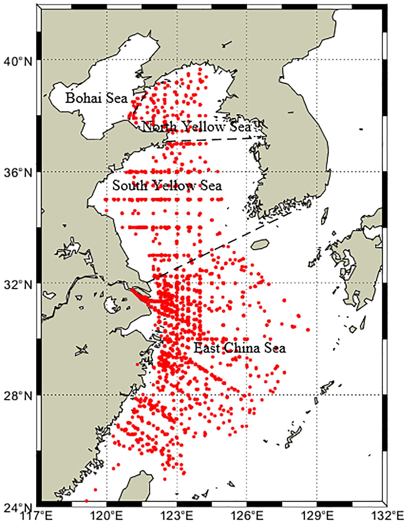
Figure 1 Distributions of in-situ stations in the YECS. The black dashed line is the dividing line between the Bohai Sea, the North Yellow Sea, the South Yellow Sea and the East China Sea.

2.2 Model building methodology

The Back Propagation neural network (BPNN) is a kind of multi-layer feed-forward neural network trained according to the error backpropagation algorithm, which belongs to one of the ANNs models. The backpropagation algorithm contains two processes, the forward propagation of the signal and the back propagation of the error (Figure 2). Forward propagation refers to the input signal (feature) applied to the output node through the hidden layer and is transformed to the output node through the nonlinear transformation that generates an output signal. When the actual output does not match the desired value, the output error is back propagated to the input layer and distributed to the neurons in each layer to obtain the error signal obtained from each layer. The error signal obtained from each layer is used as the basis for adjusting the weights of each unit. After repeated learning and training, the connection strength of each node is continuously adjusted so that the error is in the direction of the gradient direction. After repeated learning and training, the connection strength of each node is continuously adjusted so that the error decreases in the direction of the gradient, and the weights and thresholds corresponding to the minimum error are determined, to achieve the effect that the output results are close to the actual value, and the training is finished at this time (Fu et al., 2021a).

Figure 2

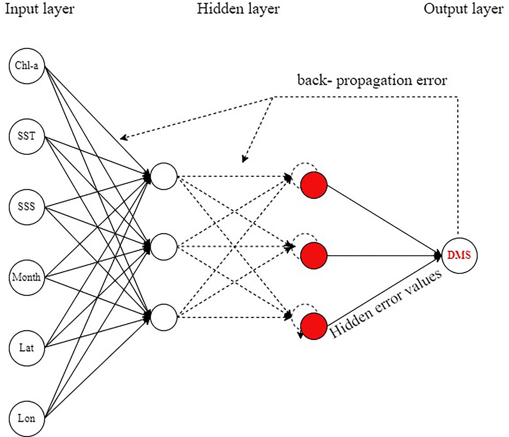
Figure 2 Structure of BP neural network.

Generally, increasing the number of neurons and the depth of the network during training can improve the learning ability of the network to extract useful information from the training set. However, the modeling dataset is only 2780 sets of data, which is a small dataset compared to the ocean database, and a neural network with too much depth and complexity will learn the features of a large amount of noisy data because of the insufficient data in the training set when it performs inversion operation, resulting in the poor generalization ability of the model and overfitting phenomenon easily. To avoid this phenomenon, one BPNN model was proposed after repeated debugging with the appropriate network depth, size, number of hidden layers, learning rate, and other parameters (Table 1). Meanwhile, a dropout layer was added in each hidden layer to ensure that some neurons can be randomly deleted during the training process, reducing the complexity and parameters of the neural network, effectively avoiding the problem of overfitting and improving the accuracy of the estimation results of the BPNN. The result accuracy is improved.

Table 1

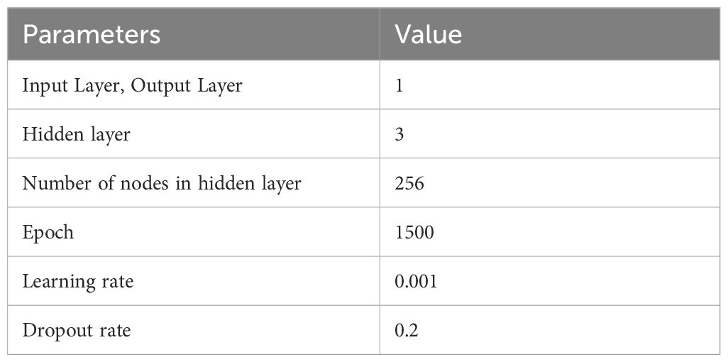
Table 1 Selected parameters of BPNN model

This study presents the BPNN of YECS constructed with the parameter combinations of time month, latitude and longitude, Chl-a, SST, and SSS, and the estimated fitting results of the DMS concentration of the surface seawater are obtained. In the construction process, the total amount of 2780 data sets was firstly divided into 2224 data training sets and 556 data test sets according to the 8:2 division ratio, and the different modeling parameters and combinations screened out were used as neurons in the input layer for the modeling algorithm, and after repeated adjustments of the algorithmic model to obtain the optimal estimation parameter scheme. The 2015 DMS-related data (300 data points) are singled out to serve as an external validation dataset for the modeling, which is to facilitate the comparison with the accuracy of related DMS forecast hindcasting methods. The remaining 2480 data sets are divided into 1984 training sets and 496 test sets according to the same partition ratio to participate in the final BPNN model weight, and the test set responses are used as the validation results of this experiment. The BPNN structure consists of one input layer, three hidden layers, and one output layer, and the input parameters are transformed by the built-in nonlinear function of the hidden layer, and the output error of the hidden layer is used as the weight adjustment to it continuously approximates to the real value of DMS concentration observation and finally outputs the DMS fitted value.

To obtain the results of BPNN estimation with optimal DMS concentration, experimental protocols EXP1-6 (Table 2) were set up and three groups of control experiments were conducted, in which the control groups EXP1 and EXP2 could explore the effect of salinity change on DMS concentration, EXP3 and EXP4 to observe the percentage of variance in DMS interpretation due to differences in temporal and spatial variations, and EXP5 and EXP6 to facilitate the comparison between the DMS cycling process of other marine factors not considered to be involved in modeling the moderating role of the three elements of chlorophyll, SST, and sea surface salinity.

Table 2

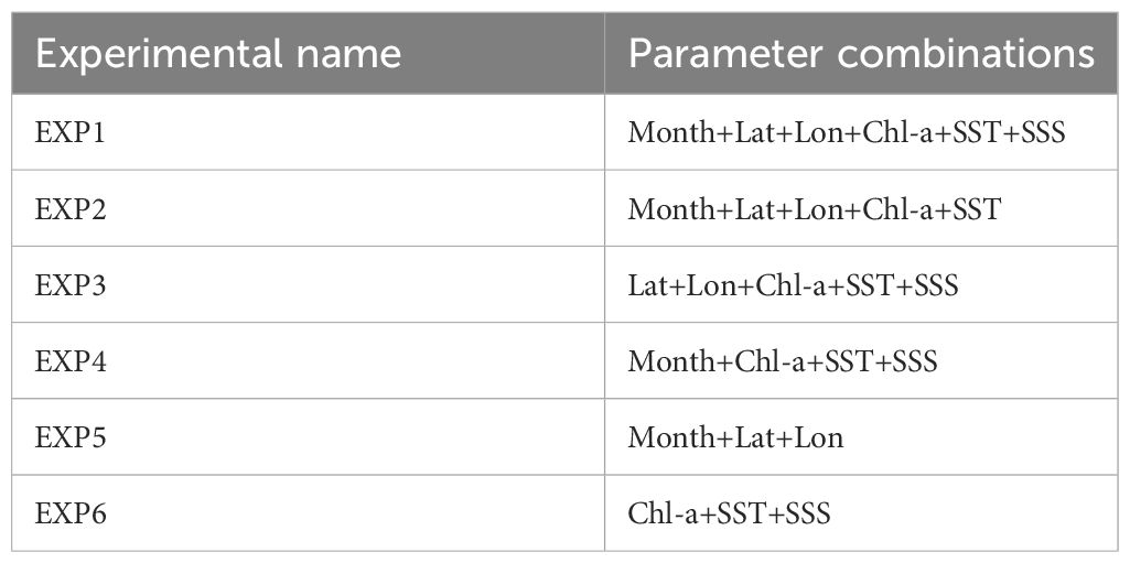
Table 2 Experimental setup of parameter combinations in BPNN model.

To evaluate the accuracy and credibility of the final reconstruction results, we used the following parameters as evaluation indicators. The coefficient of determination, R², is a statistical indicator used to assess the goodness of fit of a regression model. It indicates the proportion of variability in the dependent variable that can be explained by the model, i.e. how well the model fits the data, and could be defined as,

$$R^2=\frac{SSR}{SST}=1-\frac{SSE}{SST}$$

in which the sum of squares regression (SSR) is the sum of the difference between the predicted value and the mean of variable to quantify its variability explained by regressions model. The sum of squares of residuals (SSE) is the error between the estimate and the true value, and the sum of squares of total deviations (SST) is the error between the mean and the true value.

Both the Root Mean Squared Error (RMSE) and Mean Absolute Error (MAE) are commonly used as a measure of the difference between the predicted and measured values of a model to assess the degree of fit of the model on the given data. Theoretically, the higher the R², the smaller the MAE and RMSE, the better the model fits a dataset.

3 Results

3.1 Validation of BPNN model and its applicability analysis

Table 3 presents the evaluation parameters of the BPNN model for each experimental scheme. The algorithm was used to model the data, resulting in R² values of 0.71 for the test set. The RMSE values was 2.55 nmol/L, and the MAE values was 1.63 nmol/ L. The results of the BPNN test set constructed from the combination of EXP1 parameters demonstrate the greatest R² with MAE and RMSE values slightly higher than those of EXP2 by 10.9% and 17.0%, respectively. This discrepancy may be attributed to the discrete-valued deviation errors that affect the model's accuracy (Bell et al., 2021). These results suggest that EXP1 is the optimal parameter training combination for this study. Moreover, comparison of the R², RMSE, and MAE of all parameter experiments (Figure 3) revealed that alterations in input parameters had a positive or negative impact on model accuracy. This suggests that, in addition to temporal position, the involvement of chlorophyll, SST, and salinity in the modeling of DMS is of significance.

Figure 3

Figure 3 Validations of BPNN in the YECS. (A) EXP1, (B) EXP2, (C) EXP3, (D) EXP4, (E) EXP5, (F) EXP6. Note that r is the correlation coefficient; rMAE,rBias,rRMSE represent the relative mean error, relative bias, and relative root-mean-square error; respectively. N is the number of test samples. The color indicates the density of scattered data.

Table 3

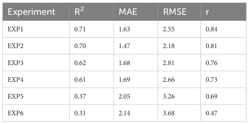
Table 3 Evaluation parameters of the DMS estimation model based on BP neural network.

To further validate the best BPNN model, the data were divided into four groups of data according to season, namely, spring (March-May), summer (June-August), autumn (September-November), and winter (December-February), to assess the seasonal applicability of the surface seawater DMS concentration in YECS. From the fit (correlation coefficient r) between the predicted values and the observations of surface seawater DMS in different seasons (Figure 4), the estimation results of the optimal BPNN model, EXP1, were better in all four seasons.

Figure 4

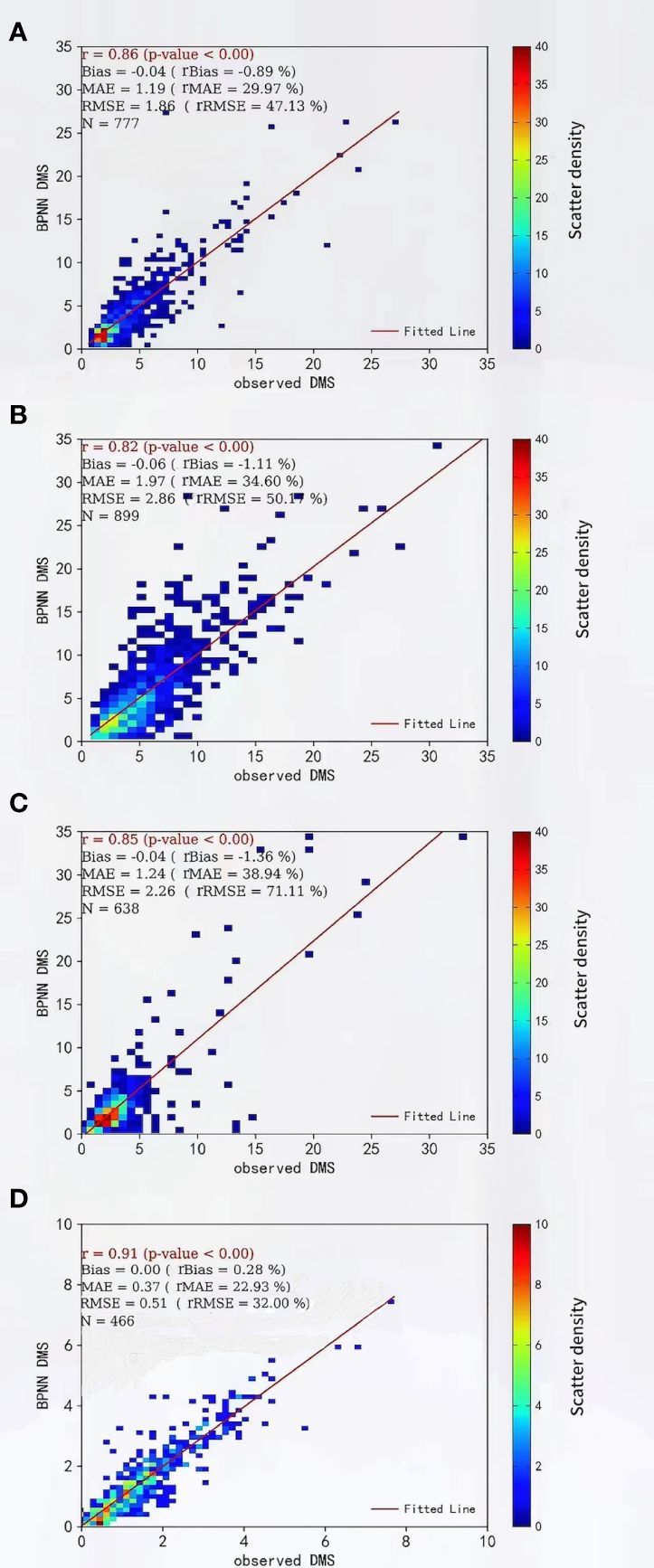
Figure 4 Seasonal applicability of DMS estimated based on the optimal BPNN in the YECS (A) Spring, (B) Summer, (C) Autumn, (D) Winter.

The MAE and RMSE of the best BPNN model were smaller in the winter, 0.37 and 0.51 nmol/L, and 1.9 and 2.86 nmol/L in the summer (Table 4), which indicated that the best BP neural network had the best applicability in the winter and the worst applicability in the summer. The MAE and RMSE of the optimal BPNN model in the four seasons did not differ much, and the explained variance of the DMS concentration in YECS exceeded 60%, which indicated that the applicability of the optimal BP neural network was still good.

Table 4

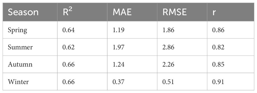
Table 4 Seasonal applicability of the best BP model.

3.2 Evaluation of DMS estimations in the YECS

Figure 5 shows the monthly DMS concentration in the YECS estimated based on the optimal BPNN model. The surface seawater DMS in the YECS exhibits pronounced seasonal variation, peaking during spring and summer and declining in autumn and winter. Particularly notable are elevated DMS concentrations in the coastal area of Changshan Islands in the North Yellow Sea and the southward sea area of the Yangtze River estuary in the East China Sea, as well as the area near Zhoushan Islands. The maximum DMS concentration typically occurs in April along the coastal area of Zhejiang and Fujian Provinces, with the fitted maximum value slightly underestimating the observed concentration by approximately 7 nmol/L (Figure 6). This discrepancy diminishes towards offshore regions. Notably, the area around Hupi Reef manifests as a hotspot for DMS concentration, reaching approximately 23 nmol/L. Similarly, elevated DMS concentrations are observed in the eastern East China Sea, aligning closely with areas of high DMS observation, particularly in proximity to Jeju Island and the Korean Peninsula, which is highly coincident with the area of high value of DMS observation (Figure 5). From the analysis of significant discrepancy in the location of Hupi Reef in April, it is suggested that in addition to the abundance of Chl-a in the spring phytoplankton population, the substantial influx of nutrients supplied to the surface by upwelling may be one of the reasons for the outbreak of DMS. In early summer, elevated DMS values were recorded in June in the North Yellow Sea near Korea Bay and Zhoushan Islands, with a broad range of high values (about 7-11 nmol/L) extending from the Yellow Sea to the western part of the East China Sea. In July, the high DMS concentrations were mainly concentrated along the coasts of Chengshanjiao and Hangzhou Bay. Compared with the observations, the fitted concentrations of DMS were relatively high in the Yangtze River estuary basin and the north-south Yellow Sea demarcation line (the coastal area of Shandong Peninsula). There were sporadic anomalously high DMS concentrations along the Yangtze River estuary in October, although the difference from the observed concentrations was large (7-10 nmol/L), the overall phenomenon in the estimated area was in perfect agreement with the conclusion of the previous studies related to DMS in autumn (anomalously high DMS in October). The DMS concentrations in the South Yellow Sea were marginally higher than the observed values (about 2-3 nmol/L) in August and November, and the model performed best in winter, with the disparity between the actual and estimated values being nearly identical to the observed values. The minimal difference between the real and estimated values is almost maintained at 0-1.50 nmol/L, suggesting that the decrease in SST coupled with a sharp decrease in Chl-a is the main reason for the low DMS in winter. These findings closely mirror the spatial and temporal distribution characteristics of the surface DMS concentration in YECS from 2005 to 2020 collected in the literature (Figure 7), which further demonstrates that the BPNN model based on the parameter combinations of EXP1 is feasible to be used for estimating the surface DMS concentration in YECS.

Figure 5

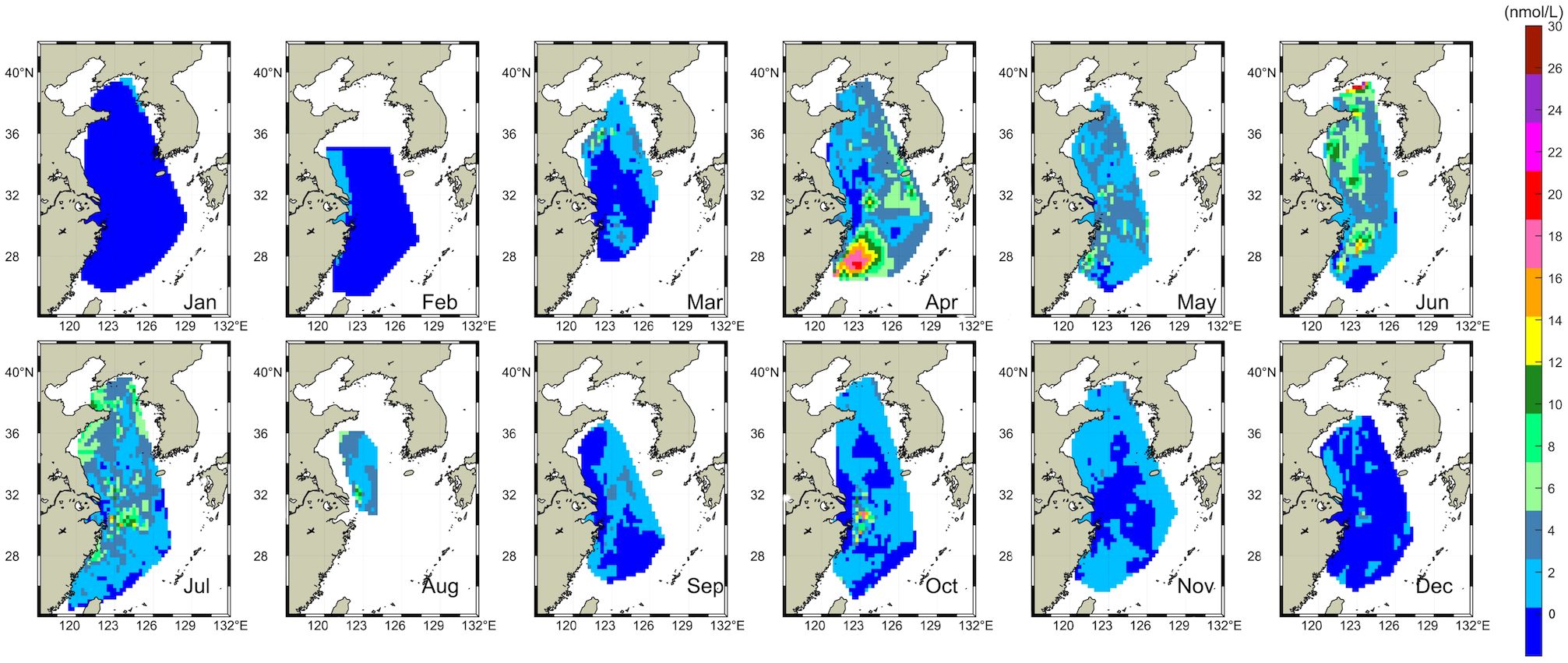
Figure 5 Monthly DMS in the YECS estimated based on BPNN.

Figure 6

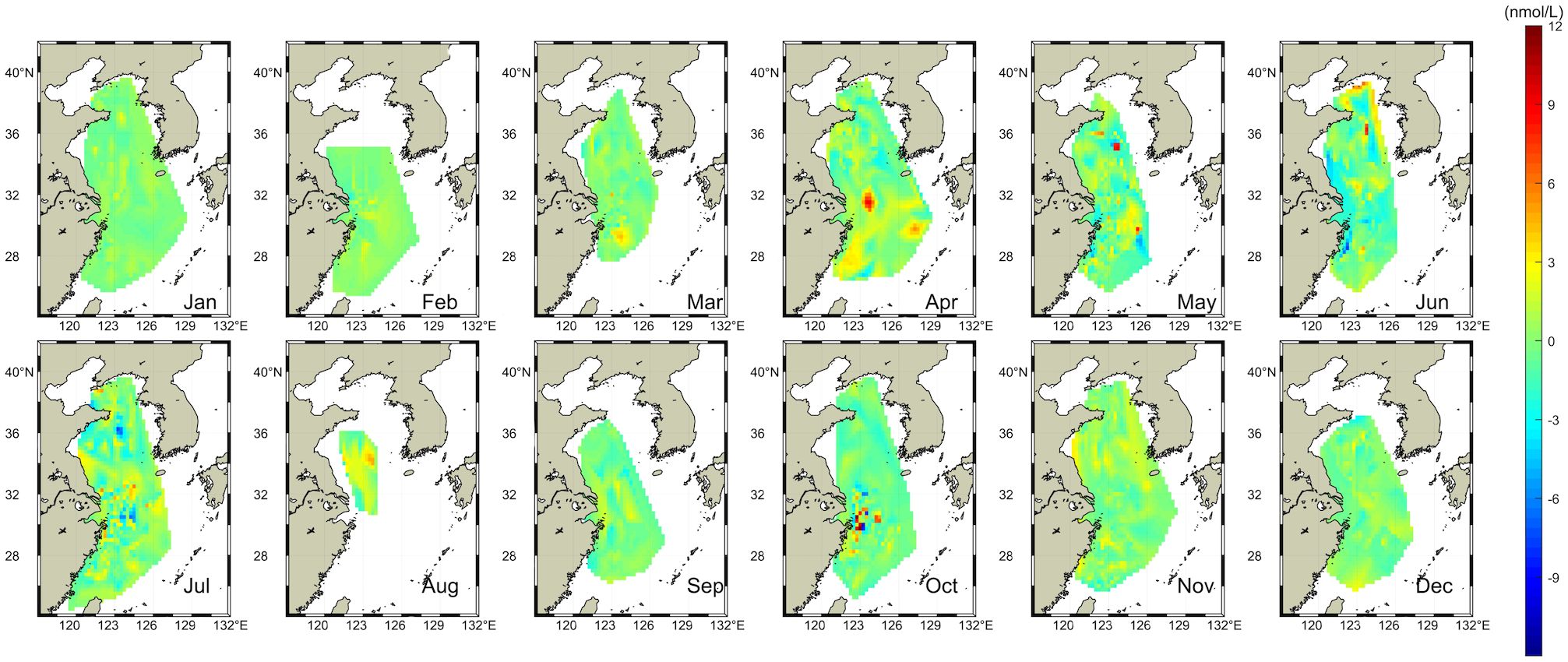
Figure 6 Difference between observed data and BPNN results from 2005 to 2020 in YECS. (Difference = Observed value - BPNN value).

Figure 7

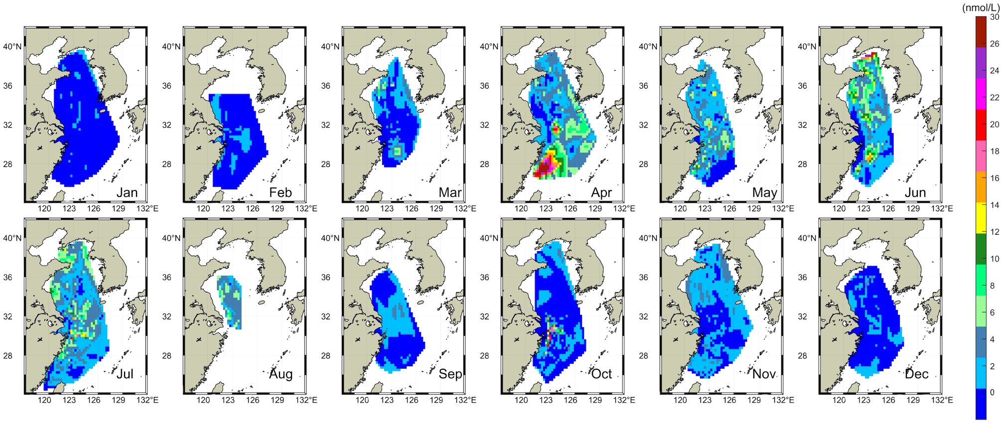
Figure 7 Seasonal distributions of monthly mean observed DMS in YECS from 2005 to 2020.

Analysis of the discrepancy between observed and estimated monthly averages (Figure 6) reveals that the majority of errors fall within the range of -2 to 1 nmol/L. Areas exhibiting minimal discrepancies are primarily situated in the Yellow Sea and the eastern East China Sea offshore waters. However, certain estimated values exhibit significant deviations, with some data points deviating by 10 nmol/L lower (in April) or 8 nmol/L higher (in June) compared to the true values. These deviations are particularly prominent in the Changjiang River mouth basin (Figure 6), with the original data points representing the extreme values. This indicates that the discrete anomalous signals of the high-concentration DMS exert a substantial impact on the accuracy and applicability of the BPNN model, which leads to a large difference in the spatial applicability of the best BPNN model in the Yellow Sea and the East China Sea. Consequently, there is a notable divergence in the spatial applicability of the optimal BPNN model in the Yellow Sea and East China Sea: the applicability is good in the offshore areas of the Yellow Sea and East China Sea, while the applicability in the extreme regions along the Yangtze River estuary and the Jeju Peninsula is relatively poor. These findings underscore the importance of considering localized environmental factors and anomalous signals when assessing the predictive performance of modeling approaches in marine ecosystems.

In general, compared with the DMS observation data, the optimal BPNN model developed in this paper has better applicability in the spatial and temporal distribution characteristics of DMS in the YECS, which may be related to the spatial and temporal information of month and latitude/longitude as the predictor variables. Although the parameters considered in this paper are not comprehensively compared with the models based on various ocean physicochemical properties such as MLD, photosynthetically active radiation (PAR) (Galí et al., 2018), upwelling, and phytoplankton abundance, the parameters required by this model are easy to obtain, and the methodology is relatively simple, and it is also able to accurately analyze the seasonal characteristics of the DMS in the surface layer of YECS and the overall trend of changes.

In addition to the comparing the BPNN model’s performance with the original observation data, to better evaluate the estimation ability of the BP model, this study compares the hindcast results with other statistical models commonly used in similar studies. Like the generalized mixed additive statistical model (GAMM) and multivariate statistical methods based on the same DMS dataset and parameter combinations. Li et al. (2023a) employed the GAMM model to obtain the hindcast DMS dataset of the East China Sea, in which the GAMM model DMS concentration was set as the response variable, and other parameters (longitude, latitude, month, SST, and Chl-a) were set as the explanatory variables. Validation of the GAMM model against the 2015 East China Sea DMS measured data yielded a correlation coefficient of 0.65 and RMSE= 0.59 nmol/L. Shen et al. (2019) established a suitable multivariate statistical model for surface DMS concentration in the Chinese offshore based on the same combination of parameters and obtained R² = 0.55 and RMSE=2.24nmol/L. Despite the significant differences in accuracy reported by various models when applied to DMS dataset in YECS, the correlation coefficient of the present experiment after external validation was obtained as r=0.95, RMSE=1.64 nmol/L, and the estimation results of the optimal BPNN, R² = 0.71 and RMSE=2.55nmol/L in our study. It indicates superior accuracy compared to the aforementioned evaluation metrics. This reaffirms the BPNN model’s efficacy in estimating DMS concentration in YECS.

4 Discussion

4.1 Spatial and temporal variations of DMS

Seasonal variations of sea surface temperature (SST), salinity (SSS), chlorophyll (Chl-a) concentration, and DMS concentration obtained based on in situ observations from 2005 to 2020 are given in Figure 8. Without considering the inter-annual and intra-seasonal variations of biogenic substances, the surface DMS concentration in YECS showed obvious seasonal variations, which started to increase in March, peaked in April and June, and gradually decreased to a low peak in autumn and winter. The highest value of DMS concentration, 41.21 nmol/L, appeared in April 2017, and its concentration was 41.19 nmol/L in mid-July 2011. It is interesting to note that there were many high values of DMS in the summer and autumn seasons, which led to the fact that the June, July, and October standard deviation of DMS concentration was slightly larger than other months, and the minimum DMS concentration of 0.03 nmol/L existed in December 2009.

Figure 8

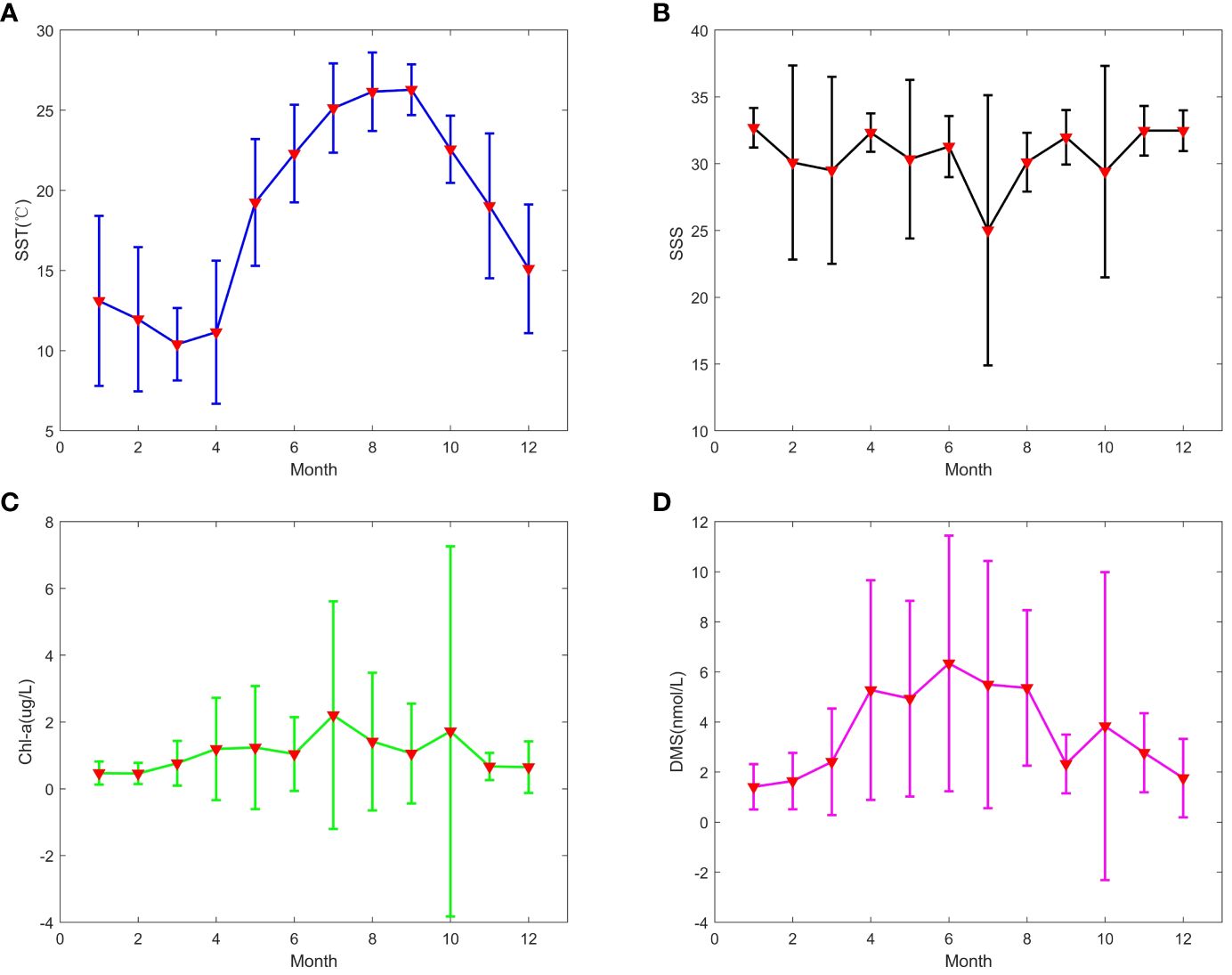
Figure 8 Seasonal variations of SST (A),salinity (B),chlorophyll (C) and DMS (D) in YECS.

The seasonal variation of DMS concentration in the YECS were similar to those of Chl-a concentration and SST (Figure 8), with positive correlations (correlation coefficients r = 0.31, 0.23) and some negative correlations (correlation coefficients r = -0.12) with salinity. Seasonal variations of DMS were characterized by a maximum in summer, followed by a minimum in winter (summer > spring > autumn > winter), with average concentrations of 5.69, 3.96, 3.18, and 1.60 nmol/L, respectively, in all seasons. The lower concentrations of DMS in winter compared to spring and summer are due to reduced solar radiation, resulting in lower sea surface temperatures and decreased phytoplankton activity and productivity. This, in the aggregate, leads to lower SSTs and lower phytoplankton activity and productivity, with a corresponding decrease in zooplankton predation (Yu et al., 2015). It also diminished the rate of DMS secretion from DMSP, resulting in a correspondingly lower peak DMS concentration.

Since DMS and DMSP originate from seaweeds, phytoplankton species and biomass are considered to be important factors in controlling seawater DMS and DMSP concentrations (Liu et al., 2022). The size of phytoplankton biomass can directly influence the concentration of DMS in marine areas. So the main reason for the high DMS in summer and autumn is the rapid reproduction and efficient production of phytoplankton, but the algal species that cause the change of DMS during the high production period in summer and autumn are different in different sea areas. Previous authors have extensively studied the contribution of different algal species in releasing DMSP and DMS content. Their findings suggest that dinoflagellates, golden algae, and methanogens are high producers of DMS (Ma and Yang, 2023), while diatoms and cryptophytes are low producers of DMS (Yang et al., 2012). According to the research, the highest intracellular DMSP content was found in Hirschsprungia (golden algae) at 689 ± 81 mmol L^-1, followed by Anterior Gourami (dinoflagellates) at 666 ± 0 mmol L^-1, and Streptophyta (diatoms) at only 9 ± 1 mmol L^-1 (Liss et al., 1994). Additionally, Nudibranchs, which are unicellular organisms distinct from algae, have a much higher DMS production capacity than diatoms due to their higher cellular DMSP content and DMSP lyase activity (Guo et al., 2022).

Consequently, the higher DMS production capacity of phytoplankton in the East China Sea in summer than in autumn is mainly related to the dominance of methanotrophs in phytoplankton abundance (Yang et al., 2008). On the one hand, the proportion of DMS-producing methanotrophs increased with the temperature rise (Zhang et al., 2014). The upwelling along the Zhejiang coast transported a large amount of nutrients to the estuary of the Yangtze River, which promoted the release of chlorophyll from phytoplankton. Suitable temperature intervals and abundant nutrients are optimal for the growth of methanotrophs in environments with high Chl-a concentrations. On the other hand, the cell abundance of dominant algal species was higher in summer compared to autumn, which was dominated by diatoms (Yang et al., 2011). Instead, the phytoplankton population was dominated by diatoms (97.8%), and the production of DMS in the autumn decreased significantly (Yang et al., 2014; Fu et al., 2021b). Although diatoms are low producers of DMS, when they have absolute dominance in phytoplankton species, they can significantly contribute to the production of these compounds. Zheng et al. (2014) report the phytoplankton community in Jiaozhou Bay is primarily composed of diatoms and flagellates, with two peaks of phytoplankton cell counts in February and October(1.108×10⁷ cell/m³ and 4.587×10⁶ cell/m³). Similarly, the abundance of phytoplankton cells detected on the northeast side of Zhoushan Islands was 1.9 × 10⁴ cells/L (Jia et al., 2017). It proves that the amount of DMS produced by large numbers of diatoms is still significant. In contrast to the East China Sea, the flagellates were the predominant algal species responsible for DMS production in the Yellow Sea. Browman et al. (2013) report a 3-fold increase in the growth rate of flagellates from 0.23 to 0.61 d^-1 between 15 and 20°C, along with almost no growth below 10°C. During the summer, the Yellow Sea experiences high temperatures (22.7 ± 3.8°C) which promote the growth and reproduction of flagellates. These organisms account for 59.6% of the total phytoplankton abundance, leading to a high production of DMS in the northern Yellow Sea. However, the decrease in seawater temperature in the autumn(16.7 ± 3.6°C)weakened its effect on DMS production. Toward spring, the temperature gradually rose and harmful algal blooms occurred frequently in the East China Sea (Yang et al., 2012). At this time, large diatoms and active flagellates dominated the high production of DMS near Hangzhou Bay in early spring and April (Figure 5).

Figure 7 illustrates the monthly average distribution patterns of DMS aboard observation data from 2005 to 2020. In the horizontal distribution, a discernible spatial trend emerges, depicting a gradual decline in DMS concentration along the Zhejiang Province coastline extending towards the open sea. This pattern is intricately linked to the substantial discharge of anthropogenic nutrient salts in the vicinity of the Yangtze River estuary. The average concentration of DMS in YECS was 3.67 nmol/L in March or early spring. Subsequently, there was a progressive rise noted in mid-spring (April), and gradually extended to the far sea, with high concentrations in the coastal area of Liaodong Peninsula and the boundary of the Bohai and Yellow Seas. Notably, a focal point of elevated DMS values emerged in the area of Hangzhou Bay located to the south of the Yangtze River mouth from 26°N-30°N, with 28°N as the center line (the range of concentrations was 26.24-35.09 nmol/L). This distribution bears resemblance to the spatial patterns of Chl-a, likely attributable to both anthropogenic nutrient inputs and phytoplankton blooms in the central Yellow Sea during spring. The zenith of DMS concentration was attained in June, reaching a peak value of 36.83 nmol/L in the northern Yellow Sea, proximate to the Changshan Islands. Additionally, heightened DMS levels were observed near the area of the mouth of the Yangtze River in the southern Yellow Sea (about 23.60 nmol/L). In September, DMS levels surpassed those in the central Yellow Sea near the Changshan Islands. Subsequently, a decline in DMS concentration commenced in September, punctuated by minor peaks in mid-autumn (October), primarily concentrated in the Yangtze River mouth and Hangzhou Bay areas, where the highest concentration recorded was approximately 37.83 nmol/L. The occurrence of these peaks is ostensibly linked to the proliferation of diatom blooms within this maritime region during autumn. In YECS, Chl-a, DMS, and SST all reached a low peak in winter, and the DMS concentration was lower than 3.65 nmol/L, with the lowest concentration of only 0.03 nmol/L. The peaks of Chl-a, DMS, and SST in YECS were all in the winter.

During the period spanning from early spring to late autumn, persistent high concentrations of dimethyl sulfide (DMS) have been consistently observed in the Yangtze River estuary basin and downstream areas of Hangzhou Bay, Zhejiang Province (Figures 5, 7). This phenomenon is primarily attributed to the discharge of nutrient salts from agricultural and industrial sources, coupled with favorable sea surface temperatures (SST), which create optimal nutrient conditions for phytoplankton proliferation. Consequently, there is a notable proliferation of phytoplankton populations, particularly dominated by diatoms and golden algae, in the vicinity of the Yangtze River mouth. This proliferation ultimately results in abnormally high DMS concentrations around the Zhoushan Islands during autumn.

Unlike environmental parameters such as Chl-a and SST, we do not believe that the level of salinity variability significantly affects the spatial distribution of DMS in YECS. The distribution characteristics of DMS in spring and summer suggest that the enrichment of DMS in the Yangtze River estuary is related to the large amount of nutrients brought by the Changjiang (Yangtze River) Diluted Water (CDW) (Yang et al., 2012) and the favorable SST (Figure 8) that accelerates phytoplankton production efficiency. Speeckaert et al. (2019) observed that the high salinity environment was not conducive to DMS release, and we also revealed no significant correlation between salinity and DMS here. First of all, the abundant nutrients provide conducive nutritional conditions for the growth of microorganisms along the Yangtze River estuary. However, with the burgeoning growth of population and heightened anthropogenic activities (agricultural and industrial runoff), a large number of organic nutrients, such as phosphate and nitrate, have been escalated into China’s estuarine and riverine systems. This influx has notably exacerbated the impact on the phytoplankton in the Yangtze River estuary in the East China Sea and other coastal seas (Walling, 2006). In spring and summer, substantial quantities of nutrients are transported by CDW into the East China Sea, leading to elevated DMS concentrations in the estuary and its proximal waters.

At the same time, the offshore of the East China Sea is affected by the oligotrophic Kuroshio and the Taiwan Warm Current (TWC), resulting in low Chl-a concentration, and correspondingly reduced DMS concentration. Secondly, suitable SST is favorable to foster heightened activity of biological enzymes (DMSP lyase in phytoplankton cells) and accelerate the rate of DMSP cleavage to DMS, while too-low or too-high seawater temperature will limit the activity of heterotrophic organisms. It is noteworthy that the anomalous deviations of high Chl-a and DMS concentrations in October were significantly larger than those in other months (Figures 7, 8), which may be attributed to the increase of Chl-a concentration due to the large amount of nutrients brought in by the upwelling along the Fujian coast and the lower SST in the autumn, which led to the occurrence of the high-value zone of DMS concentration along the Fujian coast (Hao et al., 2019). In summary, the distribution of nutrients and SST in the eastern shelf and the influence of the phytoplankton population resulted in the spatial distribution of high DMS in the Changjiang estuary and juxtaposed with a gradual decrease of DMS offshore.

4.2 Analysis of influencing factors of DMS

Light intensity, chlorophyll, SST, nutrients, mixed layer depth, and other factors are pivotal parameters of the marine ecosystems. Variations in these parameters directly affects the living environment of plankton. DMS is produced by the phytoplankton growth and demise cycle, forming the ecological cycle of DMS. The entire cycle, encompassing the release of dimethylsulfoniopropionate (DMSP) to the production and removal of DMS, is subject to modulation by diverse oceanographic factors.

Chl-a is a key pigment that serves as a marker for important phytoplankton groups, such as diatoms and seaweeds, providing a visual measure of phytoplankton biomass within specific marine regions (Fu et al., 2021b). Numerous studies, both domestically and internationally, have consistently underscored a critical relationship between Chl-a concentration, DMSP production rate, and the concentration of DMS. The rate of DMS production was found to be higher in the microlayer and closely associated with the level of chlorophyll a (Zhang et al., 2008) (correlation coefficient r = 0.8828). During the modeling process outlined in this paper, we meticulously analyzed the distinct contribution of each environmental factor. Our findings emphasized that Chl-a had the highest explained variance at 20% (R² = 0.20), followed by SST at 8% (R² = 0.08), and salinity at only 3% (R² = 0.03). This suggests that chlorophyll content has substantial impact on the surface layer of YECS DMS compared to SST and salinity. In April, the coasts of Zhejiang and Fujian witnessed a notable outbreak of DMS (Figure 7) attributable to the spring bloom and high density of Chl-a. This fostered the production of the dominant algal species of DMS, along with the large amount of nutrients carried by the upwelling, which nourished the phytoplankton abundance. The epicenter of the high value of DMS was concentrated along the coast of Zhejiang and Fujian. During the spring and summer seasons in the Yellow Sea, when the Chl-a concentration is low, the dominance of diatoms in the phytoplankton community is relatively waned. Meanwhile, the proportion of methanogens and other algae in the phytoplankton community is instead high. The correlation between the surface DMS concentration and the Chl-a concentration in the two seasons is 0.46 and 0.48, respectively (Shen et al., 2021).

Yang et al. (2014) comprehensively explores the impact of temperature, nutrients, and other factors on the distribution of DMS, as well as its production and consumption rates in the highly productive waters of YECS. Favorable temperatures play a pivotal role in facilitating the growth of phytoplankton, with zooplankton abundance peaks occurring under moderate temperatures alongside ample food availability. Daphnia magna emerges as a significant species in YECS ecosystem. The intensified predation of Daphnia magna increases significantly within the temperature range of 15~25°C, and the concentration of DMS is elevated (Yu et al., 2015). At higher concentrations of CO₂ and temperatures, bacterial production of DMS may decrease, leading to a decrease in DMS concentration (Yan et al., 2023). The decrease in the spatial extent of high DMS concentration, alongside their migration towards the eastern shelf coast during the transition from June to July, may indeed be linked to the increase in SST.

The relationship between salinity and DMS production is somewhat controversial. Gao et al. (2017) reported a significant positive correlation between DMS and Chl-a, temperature, and salinity in the Yangtze River estuary during winter (Correlation coefficient between salinity and DMS is r=0.414). However, during summer, the correlation between salinity and DMS was not as pronounced (r=0.060) in this research. Conversely, Guo et al. (2022)calculated a statistically significant negative correlation (r= -0.236) between DMS and salinity in the Bohai and North Yellow Seas in summer. Li et al. (2015) concluded that the surface salinity of the North Yellow Sea during winter did not significantly influence the productivity and consumption rate of DMS. It is noteworthy that DMS production tends to be lower during winter, as evidenced by the overall DMS concentration in YECS, which typically ranges from 0.07-3.65 nmol/L (Figure 7). Furthermore, the salinity remains stable within the range of (33-34) during this season. The observed strong correlation between DMS and salinity in the Yangtze River estuary during winter can be attributed to the reduction of biological activity on the sea surface caused by low SST and high salinity, which due to current systems such as the CDW and TWC. Yet, it is crucial to acknowledge that this correlation does not take into account the internal interaction of environmental elements. Our study found no significant correlation between the overall surface salinity and DMS concentration in YECS. This conclusion was drawn based on the negative correlation between the monthly mean salinity and DMS concentration from 2005 to 2020, the minimal difference between the indicators of EXP1 and EXP2 in the BP model (Table 3), and the results of the sensitivity tests of the individual environmental factors.

Moreover, it is crucial to note that while most disparities between BPNN estimates and observations fell within minimal margins (0-2 nmol/L) (Figure 6), the occurrence of extreme DMS values during specific months (April, May, June, and October) underscores the necessity of considering a broader range of environmental factors beyond those examined in this study. This discrepancy likely stems from the intricate interplay of physical, chemical, and biological processes within near-shore regions. The concentration of DMS is influenced not only by variables such as Chl-a, SST, and SSS (which were incorporated into the modeling) but also by factors like nutrient concentration, upwelling dynamics (Mansour et al., 2023), ENSO phenomena and the depth of the mixed layer (MLD), among others.

For instance, the Zhoushan fishery, situated in a well-developed upwelling zone along Zhejiang Province’s coast, experiences nutrient-rich seawater upwelling from the deep sea’s lower layers to the ocean’s upper layer. This continuous nutrient influx sustains phytoplankton growth, leading to enhanced DMS production in the vicinity of Zhoushan. The slightly lower estimated DMS concentration along the Zhejiang and Fujian coasts in March and April, compared to the original observed concentrations, may be associated with this phenomenon (Figure 6). The variability of DMS emission fluxes associated with ENSO primarily arises from heightened wind speeds during La Niña events. High-frequency ENSO impacts positively the sea-air exchange fluxes of DMS (Xu et al., 2016), potentially eliciting a favorable response of DMS concentrations in the East China Sea to ENSO occurrences in the Pacific Ocean. The oceanic mixing layer serves as a reservoir for a considerable amount of heat generated by diverse dynamical processes. When the mixing layer depth is relatively shallow, a positive correlation is observed between mixing depth and nutrient concentrations. As the mixing layer deepens, the nutrient layer replenishes the upper ocean with increased nutrients, thereby augmenting chlorophyll responses. The elevated DMS concentration in the low/mid-latitude region is propelled by the combination of shallow MLD and intense irradiance (Wang et al., 2020). Situated in the subtropical low-latitude zone, the Yangtze River estuary basin experiences low cloud cover and high light intensity during summer. The MLD in this region is influenced by the CDW and the Kuroshio, both of which contribute to MLD deepening. Variations in these factors may trigger DMS outbreaks along the Yangtze River estuary coast during the summer months (Figure 5).

5 Conclusions

Based on the BPNN algorithm, a new method for estimating surface seawater DMS of the YECS is proposed by utilizing the physicochemical parameters. The spatiotemporal variations of the DMS were analyzed and the environmental factors influencing on DMS was discussed, leading to the following key conclusions:

(1) The surface DMS in YECS can be optimally estimated utilizing the seawater BPNN model, exhibiting the highest explainable variance (71%) and superior simulation accuracy. The model incorporates six crucial parameters: month, latitude, longitude, Chl-a, SST, and SSS.

(2) Sensitivity tests underscored the predominant role of Chl-a in influencing DMS levels in YECS surpassing the impact of SST and salinity. As the foremost parameter shaping DMS response, the mechanistic underpinnings of Chl-a should be prioritized in DMS forecasting and hindcasting studies. A comparative evaluation of BPNN model performance across different parameter combinations of reveals that the effect of salinity on DMS concentration in YECS is negligible.

(3) The concentration of DMS in the YECS was influenced by a confluence of environmental factors and precursor biomass. It was positively correlated with Chl-a and SST, while displaying a negative correlation with SSS. Leveraging the optimal model, we scrutinized the spatial and temporal distribution of DMS concentrations in YECS. The results delineated higher DMS concentrations during spring and summer compared to autumn and winter. Specifically, elevated concentrations of DMS were higher in the coastal waters(121°-123°E, 27°-28°N) and (124°-127°E, 29°-32°N) during spring, with coastal regions exhibiting higher concentrations relative to that of the open sea. Moreover, a discernible gradient of decreasing DMS concentrations was noted from the Yangtze River estuary towards offshore regions.

(4) The model developed in this paper aligns with existing literature regarding seasonal variations and spatial distributions. However, the estimation error is exacerbated by the intricate interplay of physical, chemical, and biological processes impacting the surface DMS concentration in near-shore waters. In addition to incorporating Chl-a, SST, SSS, time, and location information, this study recommends further exploration of physicochemical parameters such as photosynthetically active radiation(PAR), nutrient concentration, MLD, ENSO, and other relevant factors in the modeling framework.

Data availability statement

The dataset in this study are observational data and are not available to the public. Requests to access the datasets should be directed to Guo Wenning, 358120152@qq.com.

Author contributions

GW: Conceptualization, Data curation, Formal analysis, Funding acquisition, Investigation, Methodology, Project administration, Resources, Software, Supervision, Validation, Visualization, Writing – original draft, Writing – review & editing. SQ: Formal analysis, Funding acquisition, Project administration, Resources, Supervision, Validation, Writing – review & editing. WS: Validation, Writing – review & editing. ZZ: Validation, Writing – review & editing.

Funding

The author(s) declare financial support was received for the research, authorship, and/or publication of this article. This project was supported by National Key Research and Development Program of China (2023YFC3108203) and Laoshan Laboratory Science and Technology Innovation Program (LSKJ202202104).

Acknowledgments

We would like to thank Prof. Liang Zhao and his team at the Physical Oceanography Laboratory for their support and help. We would like to thank Jia-Wei Shen for organizing and providing the observation data.

Conflict of interest

The authors declare that the research was conducted in the absence of any commercial or financial relationships that could be construed as a potential conflict of interest.

Publisher’s note

All claims expressed in this article are solely those of the authors and do not necessarily represent those of their affiliated organizations, or those of the publisher, the editors and the reviewers. Any product that may be evaluated in this article, or claim that may be made by its manufacturer, is not guaranteed or endorsed by the publisher.

References

Andreae M. O. (1990). Ocean-atmosphere interactions in the global biogeochemical sulfur cycle. Mar. Chem. 30, 1–29. doi: 10.1016/0304-4203(90)90059-L

CrossRef Full Text | Google Scholar

Archer S. D., Kimmance S. A., Stephens J. A., Hopkins F. E., Bellerby R. G. J., Schulz K. G., et al. (2013). Contrasting responses of DMS and DMSP to ocean acidification in Arctic waters. Biogeosciences 10, 1893–1908. doi: 10.5194/bg-10-1893-2013

CrossRef Full Text | Google Scholar

Ayers G. P., Ivey J. P., Gillett R. W. (1991). Coherence between seasonal cycles of dimethyl sulphide, methanesulphonate and sulphate in marine air. Nature 349, 404–406. doi: 10.1038/349404a0

CrossRef Full Text | Google Scholar

Bell T. G., Porter J. G., Wang W.-L., Lawler M. J., Boss E., Behrenfeld M. J., et al. (2021). Predictability of seawater DMS during the North Atlantic aerosol and marine ecosystem study (NAAMES). Front. Mar. Sci. 7. doi: 10.3389/fmars.2020.596763

CrossRef Full Text | Google Scholar

Browman H., Boyd P. W., Rynearson T. A., Armstrong E. A., Fu F., Hayashi K., et al. (2013). Marine phytoplankton temperature versus growth responses from polar to tropical waters – outcome of a scientific community-wide study. PloS One 8, 63091–63108. doi: 10.1371/journal.pone.0063091

CrossRef Full Text | Google Scholar

Challenger F., Simpson M. I. (1948). Studies on biological methylation; a precursor of the dimethyl sulphide evolved by Polysiphonia fastigiata; dimethyl-2-carboxyethylsulphonium hydroxide and its salts. Biochem. J. 3, 1591–1597. doi: 10.1039/jr9480001591

CrossRef Full Text | Google Scholar

Charlson R. J., Lovelock J. E., Andreae M. O., Warren S. G. (1987). Oceanic phytoplankton, atmospheric sulphur, cloud albedo and climate. Nature 326, 655–661. doi: 10.1038/326655a0

CrossRef Full Text | Google Scholar

Fu X., Liu W., Hu H. (2021a). Remote sensing inversion modeling of chlorophyll-a concentration in Wuliangsuhai Lake based on BP neural network. JPCS 1955, 012103–012109. doi: 10.1088/1742-6596/1955/1/012103

CrossRef Full Text | Google Scholar

Fu X., Sun J., Wei Y., Liu Z., Xin Y., Guo Y., et al. (2021b). Seasonal shift of a phytoplankton (>5 µm) community in Bohai Sea and the adjacent Yellow Sea. Diversity 13, 65–84. doi: 10.3390/d13020065

CrossRef Full Text | Google Scholar

Fung K. M., Heald C. L., Kroll J. H., Wang S., Jo D. S., Gettelman A., et al. (2022). Exploring dimethyl sulfide (DMS) oxidation and implications for global aerosol radiative forcing. Atmos. Chem. Phys. 22, 1549–1573. doi: 10.5194/acp-22-1549-2022

CrossRef Full Text | Google Scholar

Galí M., Levasseur M., Devred E., Simó R., Babin M. (2018). Sea-surface dimethylsulfide (DMS) concentration from satellite data at global and regional scales. Biogeosciences 15, 3497–3519. doi: 10.5194/bg-15-3497-2018

CrossRef Full Text | Google Scholar

Gao N., Yang G.-P., Zhang H.-H., Liu L. (2017). Temporal and spatial variations of three dimethylated sulfur compounds in the Changjiang Estuary and its adjacent area during summer and winter. Environ. Chem. 14, 160–177. doi: 10.1071/EN16158

CrossRef Full Text | Google Scholar

Grandey B. S., Wang C. (2015). Enhanced marine sulphur emissions offset global warming and impact rainautumn. Sci. Rep. 5, 13055–13061. doi: 10.1038/srep13055

PubMed Abstract | CrossRef Full Text | Google Scholar

Guo Y., Peng L., Liu Z., Fu X., Zhang G., Gu T., et al. (2022). Study on the seasonal variations of dimethyl sulfide, its precursors and their impact factors in the Bohai Sea and North Yellow Sea. Front. Mar. Sci. 9. doi: 10.3389/fmars.2022.999350

PubMed Abstract | CrossRef Full Text | Google Scholar

Hao Q., Chai F., Xiu P., Bai Y., Chen J., Liu C.-G., et al. (2019). Spatial and temporal variation in chlorophyll a concentration in the Eastern China Seas based on a locally modified satellite dataset. Estuar. Coast. Shelf Sci. 220, 220–231. doi: 10.1016/j.ecss.2019.01.004

CrossRef Full Text | Google Scholar

Jia T., Zhang H.-H., Zhang S.-H. (2017). Concentration distribution and influencing factors of dimethyl organic sulfide in the East China Sea in fall. Mar. Environ. Sci. (in Chinese) 36, 21–28. doi: 10.13634/j.cnki.mes.2017.01.004

CrossRef Full Text | Google Scholar

Keller M. D., Bellows W. K., Guillard R. R. L. (1989). Dimethyl sulfide production in marine phytoplankton. J. Am. Chem. Soc., 167–182. doi: 10.1021/bk-1989-0393.ch011

CrossRef Full Text | Google Scholar

Kettle A. J., Andreae M. O. (2000). Flux of dimethylsulfide from the oceans: A comparison of updated data sets and flux models. J. Geophys. Res. Atmos. 105, 26793–26808. doi: 10.1029/2000JD900252

CrossRef Full Text | Google Scholar

Kloster S., Feichter J., Maier-Reimer E., Six K. D., Stier P., Wetzel P. J. B. (2005). DMS cycle in the marine ocean-atmosphere system – a global model study. Biogeosciences 3, 29–51. doi: 10.5194/bgd-2-1067-2005

CrossRef Full Text | Google Scholar

Kloster S., Six K. D., Feichter J., Maier-Reimer E., Roeckner E., Wetzel P., et al. (2007). Response of dimethylsulfide (DMS) in the ocean and atmosphere to global warming. J. Geophys. Res-biogeo. 112, 3005–1-3005-13. doi: 10.1029/2006JG000224

CrossRef Full Text | Google Scholar

Li S. Y., Sun Q., Guo W. (2023a). Variability of DMS in the East China Sea and its response to different ENSO categories. Ecol. Indic. 147, 109963–109972. doi: 10.1016/j.ecolind.2023.109963

CrossRef Full Text | Google Scholar

Li S. Y., Sun Q., Yao J., Zhao L. (2023b). Characterization of spatial and temporal variations of dimethyl sulfide in the East China Sea and analysis of influencing factors. Chin. Environ. Sci. (in Chinese) 43, 2470–2479. doi: 10.19674/j.cnki.issn1000-6923.20230104.015

CrossRef Full Text | Google Scholar

Li C.-X., Yang G.-P., Wang B.-D. (2015). Biological production and spatial variation of dimethylated sulfur compounds and their relation with plankton in the North Yellow Sea. Cont. Shelf Res. 102, 19–32. doi: 10.1016/j.csr.2015.04.013

CrossRef Full Text | Google Scholar

Li F., Zhao L., Shen J. W., Yao J., Wang S. (2022). Modeling and analysis of DMS concentration changes in the Yellow Sea under the future RCP4.5 scenario. Chin. Environ. Sci. (in Chinese) 42, 4304–4314. doi: 10.19674/j.cnki.issn1000-6923.20220507.005

CrossRef Full Text | Google Scholar

Liss P. S., Hatton A. D., Malin G., Nightingale P. D., Turner S. M. (1997). Marine sulphur emissions. Philos. Trans. R. Soc B 352, 159–169. doi: 10.1098/rstb.1997.0011

CrossRef Full Text | Google Scholar

Liss P. S., Malin G., Turner S. M., Holligan P. M. (1994). Dimethyl sulphide and Phaeocystis: A review. J. Mar. Syst. 5, 41–53. doi: 10.1016/0924-7963(94)90015-9

CrossRef Full Text | Google Scholar

Liu C.-Y., Han L., Wang L.-L., Li P.-F., Yang G.-P. (2022). Dimethylsulfoniopropionate, dimethylsulfide, and acrylic acid of a typical semi-enclosed bay in the western Yellow Sea: Spatiotemporal variations and influencing factors. Mar. Chem. 245, 104159–104171. doi: 10.1016/j.marchem.2022.104159

CrossRef Full Text | Google Scholar

Ma Q.-Y., Yang G.-P. (2023). Roles of phytoplankton, microzooplankton, and bacteria in DMSP and DMS transformation processes in the East China Continental Sea. Prog. Oceanogr. 213, 103003–103016. doi: 10.1016/j.pocean.2023.103003

CrossRef Full Text | Google Scholar

Mansour K., Decesari S., Ceburnis D., Ovadnevaite J., Rinaldi M. (2023). Machine learning for prediction of daily sea surface dimethylsulfide concentration and emission flux over the North Atlantic Ocean, (1998–2021). Sci. Total Environ. 871, 162123–162136. doi: 10.1016/j.scitotenv.2023.162123

PubMed Abstract | CrossRef Full Text | Google Scholar

McNabb B. J., Tortell P. D. (2022). Improved prediction of dimethyl sulfide (DMS) distributions in the northeast subarctic Pacific using machine-learning algorithms. Biogeosciences 19, 1705–1721. doi: 10.5194/bg-19-1705-2022

CrossRef Full Text | Google Scholar

Quinn P. K., Bates T. S. (2011). The case against climate regulation via oceanic phytoplankton sulphur emissions. Nature 480, 51–56. doi: 10.1038/nature10580

PubMed Abstract | CrossRef Full Text | Google Scholar

Sarwar G., Kang D., Henderson B. H., Hogrefe C., Appel W., Mathur R. (2023). Examining the impact of dimethyl sulfide emissions on atmospheric sulfate over the continental U.S. Atmos 14, 11–19. doi: 10.3390/atmos14040660

CrossRef Full Text | Google Scholar

Sciare J., Mihalopoulos N., Dentener F. J. (2000). Interannual variability of atmospheric dimethylsulfide in the southern Indian Ocean. J. Geophys. Res. Atmos. 105, 26369–26377. doi: 10.1029/2000JD900236

CrossRef Full Text | Google Scholar

Shen J.-W. (2019). Research and Application of Dimethyl Sulfur Cycle Modeling in YECS. No. 29, 13th Street, Binhai New Area, Tianjin, China: Tianjin University of Science and Technology. Master’s Degree Dissertation. doi: 10.27359/d.cnki.gtqgu.2019.000272

CrossRef Full Text | Google Scholar

Shen J.-W., Zhao L., Wang S.-J., Li Y.-X. (2019). Multivariate analysis and modeling of dimethyl sulfide and environmental factors in the Yellow and East China Seas. Chin. Environ. Sci.(in Chinese) 39, 2514–2522. doi: 10.19674/j.cnki.issn1000-6923.2019.0300

CrossRef Full Text | Google Scholar

Shen J.-W., Zhao L., Zhang H.-H., Wei H., Guo X. (2021). Controlling factors of annual cycle of dimethylsulfide in the Yellow and East China seas. Mar. pollut. Bull. 169, 112517–112525. doi: 10.1016/j.marpolbul.2021.112517

PubMed Abstract | CrossRef Full Text | Google Scholar

Speeckaert G., Borges A. V., Gypens N. (2019). Salinity and growth effects on dimethylsulfoniopropionate (DMSP) and dimethylsulfoxide (DMSO) cell quotas of Skeletonema costatum, Phaeocystis globosa and Heterocapsa triquetra. Estuar. Coast. Shelf Sci. 226, 106275–106285. doi: 10.1016/j.ecss.2019.106275

CrossRef Full Text | Google Scholar

Toole D. A., Kieber D. J., Kiene R. P., White E. M., Bisgrove J., Del Valle D. A., et al. (2004). High dimethylsulfide photolysis rates in nitrate-rich Antarctic waters. Geophys. Res. Lett. 31, 1019863–1019866. doi: 10.1029/2004GL019863

CrossRef Full Text | Google Scholar

Vogt M., Liss P. (2009). Dimethylsulfide and climate. Surface ocean-lower atmosphere processes. Geophys. Res. 187, 197–232. doi: 10.1029/2008GM000790

CrossRef Full Text | Google Scholar

Walling D. E. (2006). Human impact on land–ocean sediment transfer by the world’s rivers. Geomo 79, 192–216. doi: 10.1016/j.geomorph.2006.06.019

CrossRef Full Text | Google Scholar

Wang W.-L., Song G., Primeau F., Saltzman E. S., Bell T. G., Moore J. K. (2020). Global ocean dimethyl sulfide climatology estimated from observations and an artificial neural network. Biogeosciences 17, 5335–5354. doi: 10.5194/bg-17-5335-2020

CrossRef Full Text | Google Scholar

Xu L., Cameron-Smith P., Russell L. M., Ghan S. J., Liu Y., Elliott S., et al. (2016). DMS role in ENSO cycle in the tropics. J. Geophys. Res. Atmos. 121, 1–22. doi: 10.1002/2016JD025333

CrossRef Full Text | Google Scholar

Xue L., Kieber D. J., Masdeu-Navarro M., Cabrera-Brufau M., Rodríguez-Ros P., Gardner S. G., et al. (2022). Concentrations, sources, and biological consumption of acrylate and DMSP in the tropical Pacific and coral reef ecosystem in Mo’orea, French Polynesia. Front. Mar. Sci. 9. doi: 10.3389/fmars.2022.911522

PubMed Abstract | CrossRef Full Text | Google Scholar

Yan S.-B., Li X.-J., Xu F., Zhang H.-H., Wang J., Zhang Y., et al. (2023). High-resolution distribution and emission of dimethyl sulfide and its relationship with pCO2 in the Northwest Pacific Ocean. Front. Mar. Sci. 10. doi: 10.3389/fmars.2023.1074474

CrossRef Full Text | Google Scholar

Yang G.-P., Jing W.-W., Kang Z.-Q., Zhang H.-H., Song G.-S. (2008). Spatial variations of dimethylsulfide and dimethylsulfoniopropionate in the surface microlayer and in the subsurface waters of the South China Sea during springtime. Mar. Environ. Res. 65, 85–97. doi: 10.1016/j.marenvres.2007.09.002

PubMed Abstract | CrossRef Full Text | Google Scholar

Yang G. P., Song Y. Z., Zhang H. H., Li C. X., Wu G. W. (2014). Seasonal variation and biogeochemical cycling of dimethylsulfide (DMS) and dimethylsulfoniopropionate (DMSP) in the Yellow Sea and Bohai Sea. J. Geophys. Res-oceans. 119, 8897–8915. doi: 10.1002/2014JC010373

CrossRef Full Text | Google Scholar

Yang G.-P., Zhang H.-H., Zhou L.-M., Yang J. (2011). Temporal and spatial variations of dimethylsulfide (DMS) and dimethylsulfoniopropionate (DMSP) in the East China Sea and the Yellow Sea. Cont. Shelf Res. 31, 1325–1335. doi: 10.1016/j.csr.2011.05.001

CrossRef Full Text | Google Scholar

Yang G.-P., Zhuang G.-C., Zhang H.-H., Dong Y., Yang J. (2012). Distribution of dimethylsulfide and dimethylsulfoniopropionate in the Yellow Sea and the East China Sea during spring: Spatio-temporal variability and controlling factors. Mar. Chem. 138-139, 21–31. doi: 10.1016/j.marchem.2012.05.003

CrossRef Full Text | Google Scholar

Yu J., Tian J.-Y., Yang G.-P. (2015). Effects of Harpacticus sp. (Harpacticoida, copepod) grazing on dimethylsulfoniopropionate and dimethylsulfide concentrations in seawater. J. Sea Res. 99, 17–25. doi: 10.1016/j.seares.2015.01.004

CrossRef Full Text | Google Scholar

Zhang S.-H., Yang G.-P., Zhang H.-H., Yang J. (2014). Spatial variation of biogenic sulfur in the south Yellow Sea and the East China Sea during summer and its contribution to atmospheric sulfate aerosol. Sci. Total Environ. 488-489, 157–167. doi: 10.1016/j.scitotenv.2014.04.074

PubMed Abstract | CrossRef Full Text | Google Scholar

Zhang H.-H., Yang G.-P., Zhu T. (2008). Distribution and cycling of dimethylsulfide (DMS) and dimethylsulfoniopropionate (DMSP) in the sea-surface microlayer of the Yellow Sea, China, in spring. Cont. Shelf Res. 28, 2417–2427. doi: 10.1016/j.csr.2008.06.003

CrossRef Full Text | Google Scholar

Zheng S., Sun X.-X., Zhao Y.-F., Sun S. (2014). Annual variation of species composition and abundance distribution of phytoplankton in 2010 in the Jiaozhou Bay. Mar. Sci. (in Chinese) 38, 1–6. doi: 10.11759/hykx20130222002

CrossRef Full Text | Google Scholar