Impact of assimilation of absolute dynamic topography on Arctic Ocean circulation

The ocean circulation is typically constrained in operational analysis and forecasting systems through the assimilation of sea level anomaly (SLA) retrievals from satellite altimetry. This approach has limited benefits in the Arctic Ocean and surrounding seas due to data gaps caused by sea ice coverage. Moreover, assimilation of SLA in seasonally ice-free regions may be negatively affected by the quality of the Mean Sea Surface (MSS) used to derive the SLA. Here, we use the Regional Ice Ocean Prediction System (RIOPS) to investigate the impact of assimilating Absolute Dynamic Topography (ADT) fields on the circulation in the Arctic Ocean. This approach avoids the use of a MSS and additionally provides information on sea level in ice covered regions using measurements across leads (openings) in the sea ice. RIOPS uses a coupled ice-ocean model on a 3-4 km grid-resolution pan-Arctic domain together with a multi-variate reduced-order Kalman Filter. The system assimilates satellite altimetry and sea surface temperature together with in situ profile observations. The background error is modified to match the spectral characteristics of the ADT fields, which contain less energy at small scales than traditional SLA due to filtering applied to reduce noise originating in the geoid product used. A series of four-year reanalyses demonstrate significant reductions in innovation statistics with important impacts across the Arctic Ocean. Results suggest that the assimilation of ADT can improve circulation and sea ice drift in the Arctic Ocean, and intensify volume transports through key Arctic gateways and resulting exchanges with the Atlantic Ocean. A reanalysis with a modified Mean Dynamic Topography (MDT) is able to reproduce many of the benefits of the ADT but does not capture the enhanced transports. Assimilation of SLA observations from leads in the sea ice appears to degrade several circulation features; however, these results may be sensitive to errors in MDT. This study highlights the large uncertainties that exist in present operational ocean forecasting systems for the Arctic Ocean due to the relative paucity and reduced quality of observations compared to ice-free areas of the Global Ocean. Moreover, this underscores the need for dedicated and focused efforts to address this critical gap in the Global Ocean Observing System.

1 Introduction

Satellite altimeters have been providing near-global estimates of sea surface height (SSH) for the last 30 years (Abdalla et al., 2021). Satellite measurements of SSH are usually processed to account for instrumental errors and geophysical corrections. Additionally, they are referenced to a mean sea surface (MSS) to provide sea level anomalies (SLA) that are routinely assimilated in operational ocean analysis systems to constrain the mesoscale and basin-scale circulation (Le Traon et al., 2015; Tonani et al., 2015; Jacobs et al., 2021). Indeed, several studies show that it is possible to provide reliable predictions of the location and properties of ocean mesoscale eddies through this approach (e.g. Smith and Fortin, 2022).

The assimilation of satellite altimetry has limited benefits in the Arctic Ocean and surrounding seas due to data gaps caused by the presence of sea ice. However, recently developed methods (Prandi et al., 2021), now allow sea level to be estimated within leads (openings) in the ice to provide sporadic measurements of water level even in ice-infested waters. This could lead to fundamental changes in our ability to predict polar ocean circulation.

An additional challenge to assimilate satellite altimetry over the Arctic Ocean is related to the need for an MSS estimate as part of the observation processing (Pujol et al., 2018). The removal of the MSS is necessary to account for spatial variations in the geoid, which are not usually represented in numerical models that assume perfectly spherical geometry. The SLA retrievals are then assimilated in numerical models through the addition of a Mean Dynamic Topography (MDT) estimate (e.g. Rio et al., 2014) to provide an Absolute Dynamic Topography (ADT) field comparable to that produced from the model as

$\begin{array}{ll}ADT=SSH-MSS+MDT= SLA+MDT& (1)\end{array}$

This approach will be referred to hereafter as the classical approach. However, due to the seasonal variability of sea ice coverage, the MSS may be biased towards summer conditions in the Arctic Ocean, or simply unavailable in areas that are ice covered throughout the year. In addition, recent years have seen an increase in areas of open water across the Arctic Ocean in summer. As a result, the accuracy of the existing MSS and MDT solutions may be decreased in these areas, thereby limiting the potential impact of satellite altimetry in constraining sea level variability.

In the Arctic, the classical approach of retrieving ADT by first calculating SLA and then adding an MDT is therefore challenged. Over recent years, estimates of the Earth’s gravity field have been improved thanks to the launch of gravity dedicated space missions (Pail et al., 2011), such as the Challenging Minisatellite Payload (CHAMP; in 2000), the Gravity Recovery and Climate Experiment (GRACE; in 2002) and the Gravity Field and Steady-State Ocean Circulation Explorer (GOCE; in 2009). Today, thanks to the success of the GOCE mission, the marine geoid provided by the GOCE geoid models is accurate at the centimeter level at spatial scales between 100 and 125 km (Bruinsma et al., 2014). For the first time since the beginning of altimetry, it is therefore now possible to consider subtracting the geoid height from the altimeter SSH measurements directly along the altimeter tracks to provide ADT (referred to hereafter as the direct approach), as;

$\begin{array}{ll}ADT=SSH-GEOID& (2)\end{array}$

Some studies have used direct ADT to evaluate model differences from altimetry and have even demonstrated the possibility to assimilate direct ADT (e.g. Androsov et al., 2019; Xu et al., 2022). However, the seasonal presence of sea ice remains a significant limitation over the Arctic Ocean (Müller et al., 2019). Prandi et al. (2021) developed a new processing technique to use sea level observations from several satellite missions for both ice-covered and open ocean areas. Here, we build on the work of Prandi et al. (2021) and use the same input data (including three altimetry missions: SARAL/AltiKa, Sentinel-3A and Cryosat-2) but rather produce gridded fields of ADT directly using an estimate of the geoid. We then examine the impact of assimilating these direct ADT fields in a high-resolution operational ice-ocean prediction system covering the Arctic Ocean (domain shown in Figure 1). The system employed is the Regional Ice Ocean Prediction System (RIOPS; Smith et al., 2021) developed and operated by Environment and Climate Change Canada (ECCC).

Figure 1

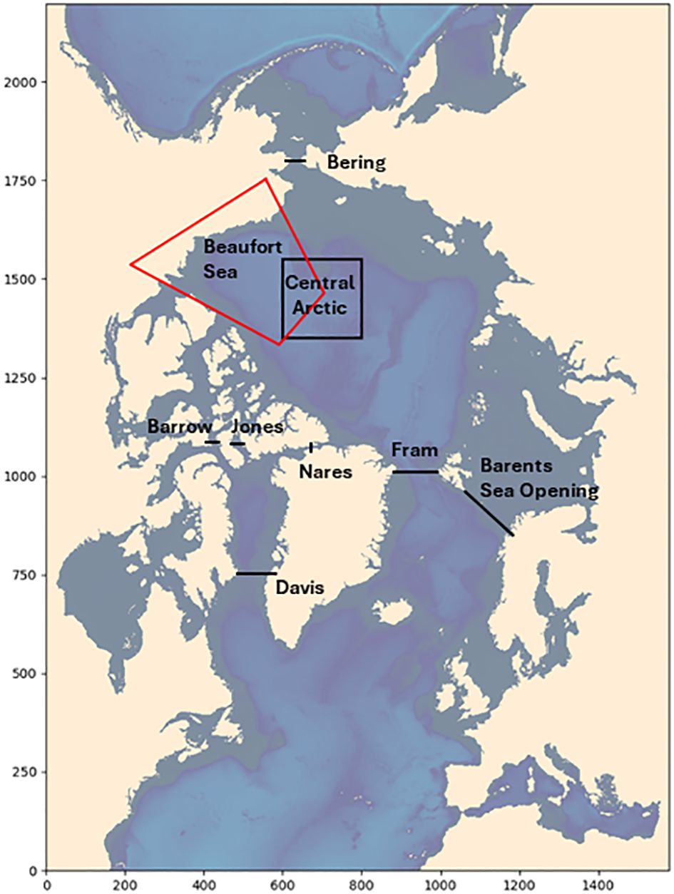
Figure 1 RIOPS model domain (shown on the model grid) extending from 26°N in the Atlantic Ocean, over the Arctic Ocean and down to 44°N in the Pacific Ocean. The central Arctic region used for power spectral density analyses is shown as a black rectangle (bounded by [75.29°N, 153.48°W], [77.94°N, 176.13°E], [80.24°N,126.77°W], [85.73°N, 166.24°W]). The Beaufort Sea region used for innovation statistics is shown as a red rectangle (bounded along latitude-longitude lines by [160°W, 123°W, 67.0°N, 80.2°N]).

The main objective of this study is to assess the impact of assimilating this ADT on surface currents and volume transports across the Arctic Ocean using a multi-year reanalysis. In particular, we aim to address the following questions:

1. What is the impact of assimilating satellite altimetry data under sea ice?

2. Do large-scale biases in the MDT affect the usefulness of assimilating satellite altimetry data in the Arctic Ocean?

3. Does the assimilation of a direct ADT have an impact on Arctic Ocean circulation features?

4. Which is more advantageous for the Arctic Ocean, assimilating a lower-resolution gridded direct ADT or a higher-resolution SLA that requires an MDT estimate?

The subsequent impact of changes in circulation on the drift of plastics throughout the Arctic Ocean is evaluated in a companion paper (Morales Maqueda et al., in prep.).

Section 2 provides a description of the methodology used to construct the direct ADT fields, including the choice of geoid, input data and Optimal Interpolation (OI) parameters, as well as a comparison with SLA fields produced by Prandi et al. (2021). An evaluation of the direct ADT fields is presented in Section 3. Section 4 provides a description of the RIOPS modelling and assimilation systems, including descriptions of several modifications to RIOPS required to make use of satellite altimetry in ice-infested areas and also to adapt the system to assimilate ADT in place of SLA. Several approaches were also examined with regards to the optimal use of the direct ADT fields. These include modifications to observation errors, “bogus” data and the filtering of background error covariance matrices. Section 5 presents an evaluation of the multi-year reanalysis produced using the assimilation of direct ADT fields, in terms of impacts on innovation statistics, circulation, sea ice drift and water level. A summary and conclusions are presented in Section 6.

2 Computation of direct ADT fields

2.1 Choice of geoid

A critical component of this study is the choice of a geoid product well-adapted for direct ADT computation. Geoids correspond to the equipotential gravity field surface. Depending on the construction, they can be separated into two categories. The “Satellite-only” geoids are calculated using only gravimetric satellite missions (such as GOCE and GRACE). GOCE provides finer-resolution measurements, with spatial resolutions of up to 100 km. “Combined” geoids are calculated by adding altimetry satellite missions to the gravimetric ones improving small scale geoid gradients.

In the polar regions, satellite observations have limited spatial coverage due to their orbits. GRACE samples up to 89°N while GOCE only provides measurements up to 83.5°N. We therefore expect a reduction in the spatial resolution of the geoid at latitudes over 83.5°N where observations from GOCE are not available.

There are various geoids available (http://icgem.gfz-potsdam.de/tom_longtime), five of which were chosen for this study: GOCO05c (Gravity Observation Combination; Fecher et al., 2017), GO_CONS_GCF_2_TIM_R6e (Zingerle et al., 2019), EGM2008 (Earth Gravitational Model; Pavlis et al., 2012), EIGEN-6C4 (European Improved Gravity Model of the Earth by New Techniques; Förste et al., 2014), and GOCO06s (Kvas et al., 2021). Table 1 summarizes the data ingested in each of these five geoids. Direct ADT fields produced using each of these geoids (methodology explained in the next section) are presented in Figure 2. The direct ADT fields are similar at basin scale showing the major ocean features of the Arctic Ocean (Beaufort Gyre and Transpolar Drift). However, at smaller scales, features in the ADT fields dependent on the geoid computation method can be seen. With the satellite-only geoids, we observe small non-physical patterns and large circular patterns for latitudes over 80°N. Fewer patterns are observed with geoids that use both satellite altimetry and in-situ data. For all the geoids, we observe non-physical patterns for latitudes over 83.5°N where there are no GOCE observations.

Table 1

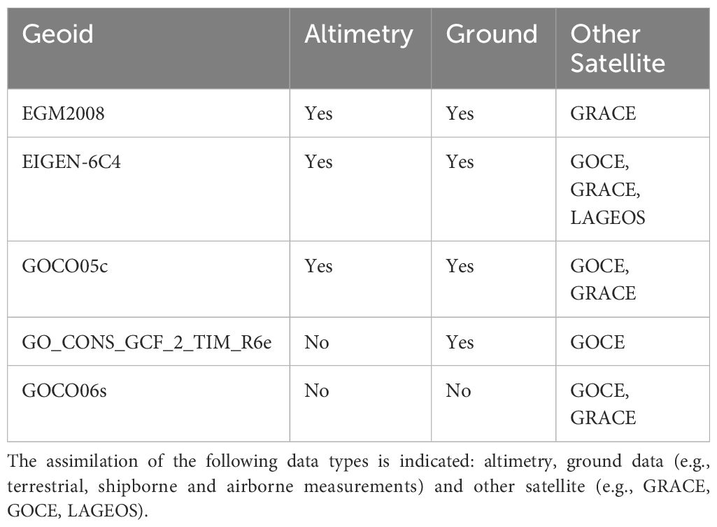
Table 1 List of the five geoids that were used for the comparisons.

Figure 2

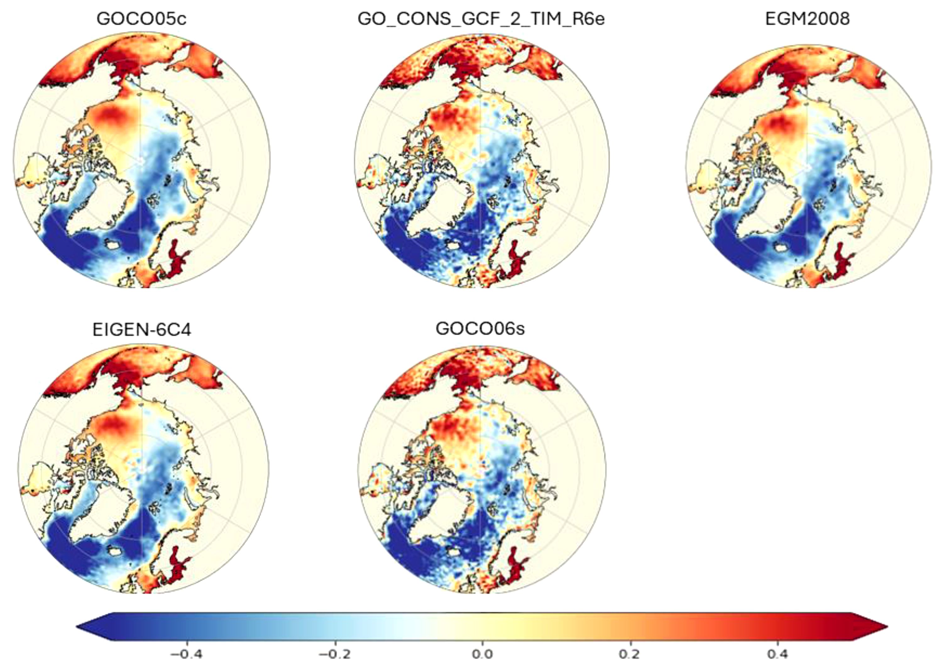
Figure 2 Satellite ADT maps (in m) on 31 December 2016 using different geoid products (from left to right: GOCO05c, GO_CONS_GCF_2_TIM_R6e, EGM2008, EIGEN-6C4, GOCO06s). The mapping procedure is described in Section 2.2.

To compute direct ADT fields, a geoid that provides the smallest variance in space with respect to the altimetry data is required to reduce residual non-physical patterns on the ADT fields. Indeed, the smoothest ADT fields are obtained with the geoids EGM-2008 and GOCO05c. Small patterns are still visible with the geoid EGM-2008 in the Beaufort and Laptev seas. We therefore use the geoid GOCO05c with the smoothest direct ADT fields for this study.

Geoid GOCO05c is constructed by ingesting both satellite altimetry data (coming from DTU13 MSS) and ground data. Therefore, this geoid is not completely independent of the input altimetry data we use for the direct ADT fields. However, its use minimizes the erroneous patterns observed with the other geoids as it is more coherent with satellite altimetry, especially for latitudes poleward of 83°N.

2.2 Production of gridded direct ADT fields

Direct ADT fields (Equation 2) are computed by combining along-track ADT data from three satellite altimeters. The characteristics of the satellite data used as inputs are summarized in Table 2. The altimetry along-track processing performed is similar to the one described in more detail in Prandi et al. (2021). It consists of classifying satellite observations corresponding to leads and open ocean, as well as editing and cross calibrating the data. The other geophysical filtering steps (e.g. for tides, dynamic atmospheric correction, etc…) are also the same as used by Prandi et al. (2021). The main difference with Prandi et al. (2021) is the removal of the geoid from the SSH to provide ADT, as opposed to the classical approach using an MSS. By applying these steps, we obtain cross-calibrated along-track ADT data from three altimetry missions from 50°N to 88°N. These data are combined through optimal interpolation (OI; Bretherton et al., 1976) to create gridded direct ADT fields. The OI scheme considers a spatio-temporal correlation scale to select along-track data around the estimation point to smooth the data and reduce geoid errors. The spatial correlation scale must be increased compared to SLA computation to take into account the geoid errors included in the direct ADT fields. GOCE spatial scale resolution is on the order of 125 km. As a result, we use a 250-km spatial correlation scale to mitigate the geoid errors and provide improved homogeneity. The temporal correlation scale is not changed from that used by Prandi et al. (2021) and is around 10 days in the Arctic Ocean.

Table 2

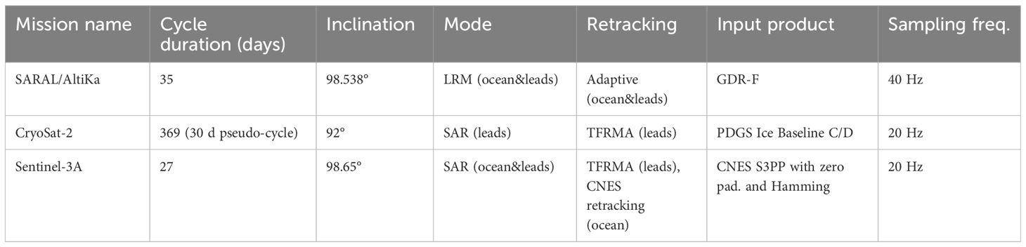
Table 2 Satellite altimetry input data characteristics.

Combining the three satellite along-track data sources through OI we obtain direct ADT fields with a grid-resolution of 25 km every 3 days for the period 07/2016 to 07/2020 covering the region from 50°N to 88°N. The map of mean ADT (not shown) shows the major dynamic topographic features of the Arctic Ocean (e.g. Transpolar Drift, Beaufort Gyre). The temporal evolution of the spatial mean (not shown) is coherent with the roughly 10 cm amplitude seasonal cycle of mean sea level in the Arctic Ocean (Armitage et al., 2016).

3 Evaluation of ADT fields

3.1 Classical ADT fields based on SLA and MDT

We compare the direct ADT fields (Equation 2) with the classical ADT fields (Equation 1) corresponding to Prandi et al. (2021) processing. Power spectral density (PSD) is computed for direct ADT and classical ADT fields (Figure 3) over the Central Arctic region (shown as a black rectangle on Figure 1). The PSD for direct ADT decreases for spatial scales below 200 km compared to classical ADT fields due to the smoothing applied to consider geoid errors and provides an indication of the effective resolution.

Figure 3

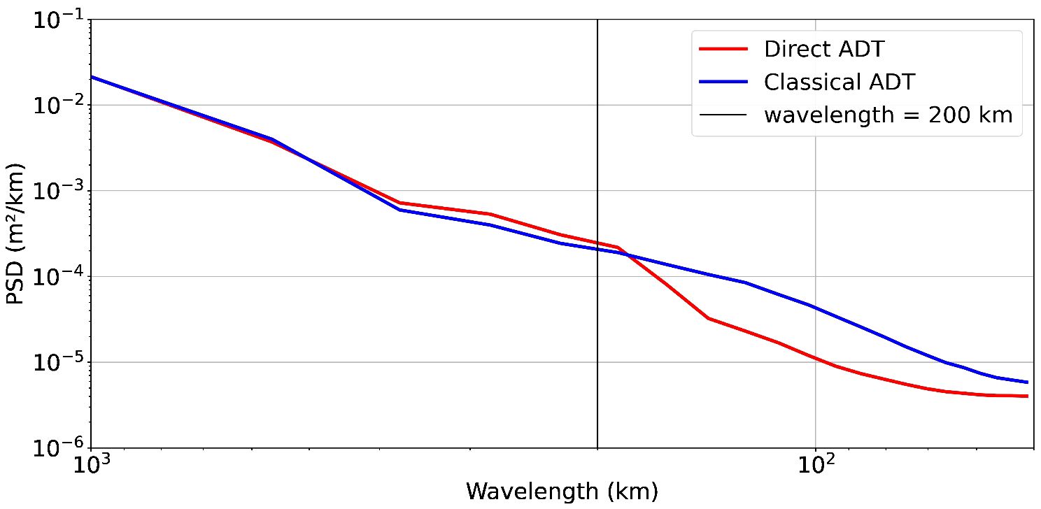
Figure 3 Power spectral density for direct ADT and classical ADT fields in the central Arctic region shown as a black rectangle in Figure 1.

Compared to classical ADT fields, direct ADT fields show increased variance north of 83°N where GOCE observations are not available and where geoid errors remain present (Figure 4). For these latitudes, the GOCO05C geoid uses information from satellite altimetry and ground data to reduce geoid errors. However, there are still residual errors (not shown) compared to the ones present in MSS and MDT fields (i.e. those assimilating satellite altimetry data up to 88°N). The variance of the direct ADT fields is also increased in a small area south of the new Siberian islands (near the strait between Laptev and East Siberian Seas). Differences between the MSS and the geoid are observed in this region (not shown) possibly indicating geoid errors. Differences between the GOCO05C geoid and other geoids don’t show any significant differences. Therefore, this indicates that the same increased variance should be expected with other geoids.

Figure 4

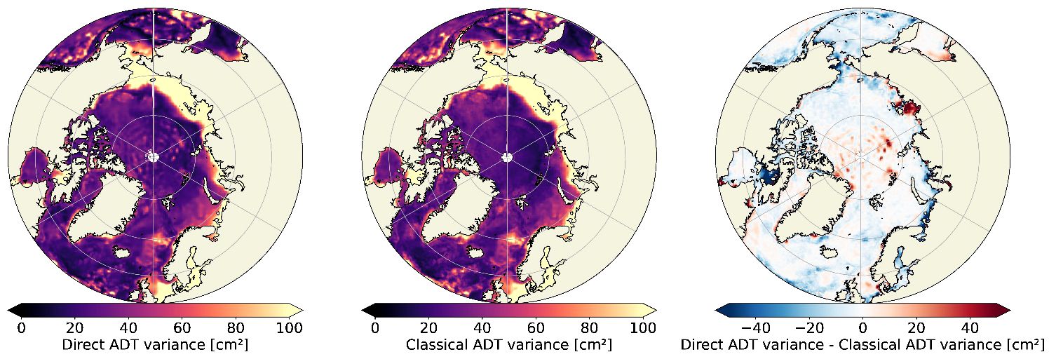
Figure 4 Temporal variance of the ADT fields (left), the classical ADT maps (middle) and the difference (right).

3.2 Tide gauge data

In-situ observations are scarce in the seasonally ice-covered Arctic Ocean. Here, we selected one Gloss/Clivar tide gauge (TG) at Prudhoe Bay where there are hourly data covering the study period in a seasonally ice-covered region (Caldwell et al., 2015). To compare to sea level from satellite altimetry, the TG sea level is corrected for the ocean tide, the Dynamical Atmospheric Correction and for the glacial isostatic adjustment (accounting for the ongoing movement of land). The corrected tide gauge sea level is compared to the altimetry ADT fields averaged 50 km around the TG. The timeseries are plotted in Figure 5. Direct ADT is well correlated with the TG sea level at a monthly timescale, including when the region is ice-covered. Direct ADT and classical ADT timeseries show similar correlations with the TG timeseries. The correlation and standard deviation of the differences between the altimetry and the in-situ time series show a slightly better agreement for the classical ADT product compared to the direct ADT product, due likely to the higher spatial resolution of the classical ADT fields.

Figure 5

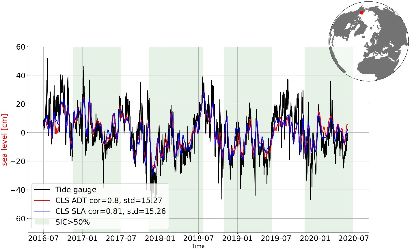
Figure 5 Comparison of sea level from altimetry from direct ADT (red) and classical ADT fields (blue) with Prudhoe Bay tide gauge sea level. Time periods for which the sea ice concentration (SIC) was greater than 50% are shown with a green background. The correlation and standard deviation of differences for both direct ADT and classical ADT fields with respect to the tide gauge observations is provided in the legend.

4 Ocean analysis system description

The main objective of this study is to make better use of satellite altimetry to produce a more accurate estimate of currents in the Arctic Ocean. The approach used is to modify an existing state-of-the-art operational ice-ocean analysis system to assimilate the direct ADT product (described in Section 2). The system employed is the Regional Ice Ocean Prediction System (RIOPS) version 2.2 developed and operated by Environment and Climate Change Canada (ECCC; Smith et al., 2021; Surcel Colan et al., 2021). Several modifications to the system were required (presented in Section 4.2) to make use of satellite altimetry in ice-infested areas as well as to adapt the system to assimilate ADT fields in place of SLA (together with an MDT). Several approaches were examined in regards to the optimal use of the direct ADT fields (Section 4.3). These include modifications to observation errors, “bogus” data and filtering of background error covariance matrices. Using this modified approach a multi-year reanalysis is produced that assimilates the direct ADT fields.

4.1 Description of RIOPS

RIOPS produces operational analyses and forecasts on a domain stretching from 26°N in the Atlantic Ocean, over the Arctic Ocean and down to 44°N in the Pacific Ocean (Figure 1). RIOPS products are used to support a number of operational needs such as: ice services, search and rescue, environmental emergency response, maritime safety and national defense. RIOPS uses the NEMO primitive equation ocean model (Madec et al., 2019) on the CREG12 grid (Dupont et al., 2015; Roy et al., 2015; Chikhar et al., 2019), with a nominal resolution of 3-8 km. RIOPS uses 75 vertical levels on a z-coordinate with a vertically-varying level scheme. Astronomical tides are forced at the RIOPS boundaries with self-attraction and loading terms applied. The Los-Alamos Community Ice CodE (CICE; Hunke, 2001; Lipscomb et al., 2007; Hunke and Lipscomb, 2008) sea ice model is used with 10 ice thickness categories.

The System d’Assimilation Mercator version 2 (SAM2) analysis scheme is used to constrain the ocean fields. SAM2 is a multi-variate reduced-order Extended Kalman Filter, used here to assimilate SLA, sea surface temperature (SST) along with in situ temperature and salinity profile data (e.g. Wong et al., 2020). A detailed description of SAM2 is available in Lellouche et al. (2013); Lellouche et al. (2018), with particular modifications for RIOPS provided in Smith et al. (2016); Smith et al. (2021). A brief description of relevant details is provided below.

The model background error is specified using a set of static multi-variate fields obtained from sub-monthly anomalies of a 10-year hindcast. The RIOPS delayed-mode analyses used here employ a 7-day assimilation window with analysis increments applied evenly using an Incremental Analysis Updating (IAU) approach (Bloom et al., 1996; Benkiran and Greiner, 2008). A multi-scale approach is used for temperature and salinity profiles whereby large-scale corrections from a 3DVar analysis are applied using mean innovations from the previous 4 cycles. The MDT used in the observation operator for SLA is the hybrid product described by Lellouche et al. (2018). This product combines the CNES-CLS13 MDT (Rio et al., 2014) with mean innovations calculated from a multi-decadal ocean reanalysis. An online sliding-window harmonic analysis is used to remove tidal variations as part of the observation operator for SLA (Smith et al., 2021). This approach permits non-stationary tides due to the seasonal presence of sea ice. The inverse barometer is also removed as part of the observation operator for SLA to account for the local model response to atmospheric pressure forcing. SLA observations assimilated include those typically assimilated in the operational system, namely: Cryosat2, Jason3, Saral/Altika, and Sentinel 3a/3b.

For SST, gridded L4 analyses produced by ECCC are used (Brasnett and Colan, 2016). SAM2 is also blended with a 3DVar ice analysis produced by ECCC to constrain the sea ice cover (Buehner et al., 2013, Buehner et al., 2016) using the Rescaled Forecast Tendencies method of Smith et al. (2016) to adjust the 10 ice thickness categories based on a total ice concentration increment. The L4 SST analysis is modified prior to assimilation to be equal to the freezing point of seawater (using the sea surface salinity from the previous analysis) for all points for which the sea ice concentration analysis has a value greater than 0.25. This ensures a balance between the ocean analysis and sea ice cover and avoids spurious ice melt and formation.

4.2 Adaptation of RIOPS for assimilation of direct ADT fields

In order to directly assimilate gridded L4 ADT observations within SAM2, several modifications of the system were made and evaluated. First, the system had to be adapted to assimilate ADT instead of SLA (Section 4.2.1) and the impact in ice-free waters evaluated. Next, a number of changes were required to allow for assimilation of satellite altimetry in ice-covered waters (Section 4.2.2).

4.2.1 Assimilation of ADT in ice-free waters

Before addressing impacts in ice-covered waters, it is important to first assess the impact of assimilating direct ADT fields in ice-free waters where SLA is normally used. Some impact is expected for a few reasons. First, the direct ADT is gridded (L4) rather than the along-track (L3) product currently used for SLA assimilation in RIOPS. As the direct ADT is on a 25-km grid (i.e. close to the resolution of the ocean analysis grid) no decimation (“superobbing”) of the data is required. The use of an L4 product will impact the observational coverage and number of observations though, as well as include spatially-correlated observation errors. Second, the reduced variance for small spatial scales in direct ADT (as compared to SLA) may reduce the lower limit for constrained scales in the resulting ocean analysis (e.g. Jacobs et al., 2021). Finally, in order to assimilate ADT in ice-free waters the observation operator was also modified to remove the application of the MDT used when assimilating SLA data.

4.2.2 Assimilation of altimetry under ice

In the standard version of SAM2 several approaches are used to limit the potential impact of satellite altimetry observations under ice. First, the SLA observations are rejected under ice based on an SST criterion (linear increase of observation error from -1°C to -1.7°C and rejection for SST< -1.7°C). Second, “bogus” observations with innovation values equal to zero are applied under ice to ensure the analysis does not vary from its background. To permit the assimilation of altimetry under ice, both the SST rejection criteria and bogus observations are deactivated. Note that an additional observation error is also applied to account for MDT error, with values greater than 20 cm in many areas of the Arctic Ocean. This is not applied when assimilating the direct ADT, rather the ADT observation errors described in Section 4.3.2 are applied.

To further optimize the use of direct ADT fields by RIOPS, several approaches are investigated and presented in the next section.

4.3 Optimization of ADT assimilation

To make the best use of direct ADT fields, several modifications to the assimilation system are desirable. In particular, we have investigated the potential impact of additional filtering of background error (Section 4.3.1), spatially-varying observational error for ADT (Section 4.3.2) and modification of the observation operator (Section 4.3.3).

4.3.1 Spatial filtering of background error

In RIOPS, background error is specified in terms of roughly 300 multi-variate anomalies obtained from a 10-year model simulation following the method described in Lellouche et al. (2013). Anomalies are calculated as the difference between daily-mean model outputs and a 45-day running mean. As such, they can be considered to represent the sub-monthly variability in the system. These anomalies are subsequently filtered using 49-passes of a 2D-Shapiro filter to reduce spurious fine-scale increments. This number of passes was found to be appropriate for use with conventional SLA observations (e.g. Benkiran et al., 2021).

As the direct ADT fields contain less variance than classical ADT at wavelengths less than 200 km (Figure 3), it is important to ensure innovations representative of long wavelengths do not generate spurious small-scale noise in increments of SSH, temperature, salinity and currents. As such, it would be appropriate to project innovations from ADT onto larger spatial scales only. Figure 6A shows the PSD of the direct ADT fields, innovations (observation-model differences) and background error modes over a box covering the central Arctic Ocean (as shown in Figure 1). The PSD of error modes with an additional 100, 200, 300, 400 and 500 passes are shown as well. We can clearly see how the amplitude of small-scale variability is reduced as the number of passes in increased. Indeed, the 50% response point increases from about 150 km at 100 passes to over 300 km with 400 passes. Following several experiments to examine the impact of the filtering on increments produced using these different sets of error modes, it was decided to choose an additional 100 passes (i.e. 149 in total) as the best choice for ADT. This was based partly on the fact that 50% response function falls in the target zone between 100-200 km where the largest differences are found between classical ADT and direct ADT fields (Figure 3), together with a subjective analysis of the resulting increments (not shown). We can see from the PSD of dynamic height increments (Figure 6B) produced with 100 and 200 additional passes that the variance of the increments is significantly reduced for scales below 100 km. Using 200 passes also results in a loss of variance above 200 km. Thus, filtering with 100 passes provides a reasonable compromise allowing reduced variance below 200 km with minimal impact for long length scales.

Figure 6

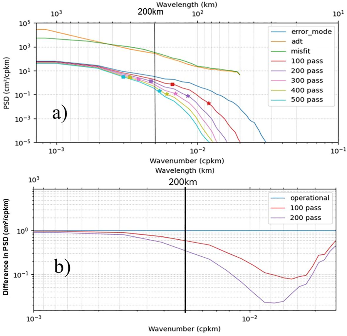
Figure 6 Power spectral density (PSD) over the central Arctic (see Figure 1) for direct ADT, misfits (innovations) with respect to direct ADT (observation-minus-model differences) and background error modes (A). Error modes are shown using operational filtering settings (49 passes), as well as with 100, 200, 300, 400 and 500 additional passes. The wavelength of the 50% and 10% response function for the various number of passes is indicated with a square and star respectively. A vertical line marks the 200 km wavelength to denote the scale at which differences between direct ADT and SLA are notable. Panel (B) shows an example of the impact of spatial filtering of error modes on the resulting PSD for an increment of dynamic height for the same region. Differences in PSD for an analysis produced with 100 and 200 additional passes (red and purple curves respectively) are shown with respect to the operational filtering of 49 passes.

4.3.2 Spatially-varying observational error for ADT

SAM2 applies spatially-varying MDT errors to altimetry observations. These are not justified for ADT and are thus set to zero. However, errors associated with the geoid (e.g. as shown in Figure 4) should be applied in place. To account for this, a spatially-varying ADT error is used that has zero error south of 80°N and an error of 20 cm north of 83°N with a linear ramp between these latitudes. The amplitude and spatial extent of this error was chosen based on differences in variance between direct ADT and classical ADT fields (Figure 4, right panel). An additional constant value of 5 cm is applied over the entire domain to account for instrument error and spatially-correlated errors from the OI procedure used to produce the gridded direct ADT. Dynamic height increments produced using these errors (not shown) result in a reduction in small-scale increments near the north pole. This reduction is desirable, as the increments are likely the result of errors in the geoid present in the direct ADT fields and not physical features.

4.3.3 Spatial filtering in the observation operator

The RIOPS ocean model has a grid resolution of 3-4 km over the Arctic Ocean and thus contains spatial variability of the SSH field at scales well below 200 km. As the model likely has more variance at these small scales than is represented in the ADT fields it should be filtered prior to calculating differences with the ADT as part of the observation operator. As a result, 49 passes of a Shapiro filter are applied to the model SSH prior to calculating differences from ADT observations. Ideally, the filtering applied in the observation operator should be equal to that applied to the background error. However, use of a consistent value (i.e. 149) was found to degrade the results somewhat. The value of 49 passes was chosen as it coincides with the number of passes usually used for the background error (Benkiran et al., 2021).

5 Evaluation of ocean reanalyses

Based on the modifications to the assimilation approach described above a multi-year reanalysis that assimilates direct ADT fields over the period Jan. 2016 to Jun. 2020 was produced (referred to hereafter as RA-ADT). This reanalysis will be evaluated as compared to a control simulation (RA-CTL) based on the operational version 2.2 of RIOPS (Surcel Colan et al., 2021). Two additional reanalyses were also produced: RA-MDT uses an identical configuration to RA-CTL but with a modified MDT; and RA-SLA uses the same configuration as RA-MDT but includes SLA under ice (updated version of Prandi et al., 2021). In RA-MDT, the MDT is adjusted based on the average SLA innovations from RA-CTL and smoothed using a Shapiro filter to roughly 5° resolution.

These four reanalyses are compared in terms of the impact on innovation statistics (i.e. observation-minus-model differences), circulation and volume transport across key Arctic gateways, sea ice drift, sea ice concentration increments, and tide gauge observations. Unless noted otherwise, all evaluation statistics are calculated over the full period of the reanalyses.

5.1 Innovation statistics

Here we present innovation statistics for assimilated observations (ADT/SLA, SST, temperature and salinity profiles) as an indication of how closely the reanalyses fit with observations. While the observation errors used are somewhat different (and this could therefore affect increments and subsequent innovations), this can nonetheless provide an indication of model skill and highlight any potential imbalances.

In order to assimilate direct ADT fields it was necessary to set the MDT to zero. As a result, for technical reasons it is not possible to cross-compare innovations between the RA-ADT and RA-CTL reanalyses. For example, it would have been useful to compare innovations of SLA in both RA-ADT and RA-CTL even if they were only assimilated in the latter (and vice-versa). As such, innovations presented here are with respect to the specific observational datasets assimilated. For RA-CTL and RA-MDT this includes global altimetry data (i.e. excluding ice covered areas) for Saral/Altika, Jason3, Sentinel3a, Sentinel3b and Cryosat2. Innovations for RA-SLA include both global and Arctic (leads) retrievals of SLA. Innovations for RA-ADT are with respect to the direct ADT fields that include both global and Arctic (leads) retrievals.

Mean innovation statistics with respect to satellite altimetry are presented in Figure 7. Significantly smaller mean innovations are found for all experiments compared to RA-CTL. In particular, the large negative innovations present in RA-CTL throughout much of the Arctic Ocean, Baffin Bay and Hudson Bay are no longer present. As expected, RA-MDT shows the smallest mean innovations overall (Figure 7C), since the updated MDT was developed to minimize mean innovations based on the global altimetry datasets against which the innovations for RA-MDT are calculated. RA-SLA uses the updated MDT but includes the Arctic (leads) product as well, which results in larger (positive) mean innovations over the Arctic coastal areas. RA-ADT is produced without using an MDT and produces mean innovations that are somewhat larger than RA-MDT but smaller than RA-CTL.

Figure 7

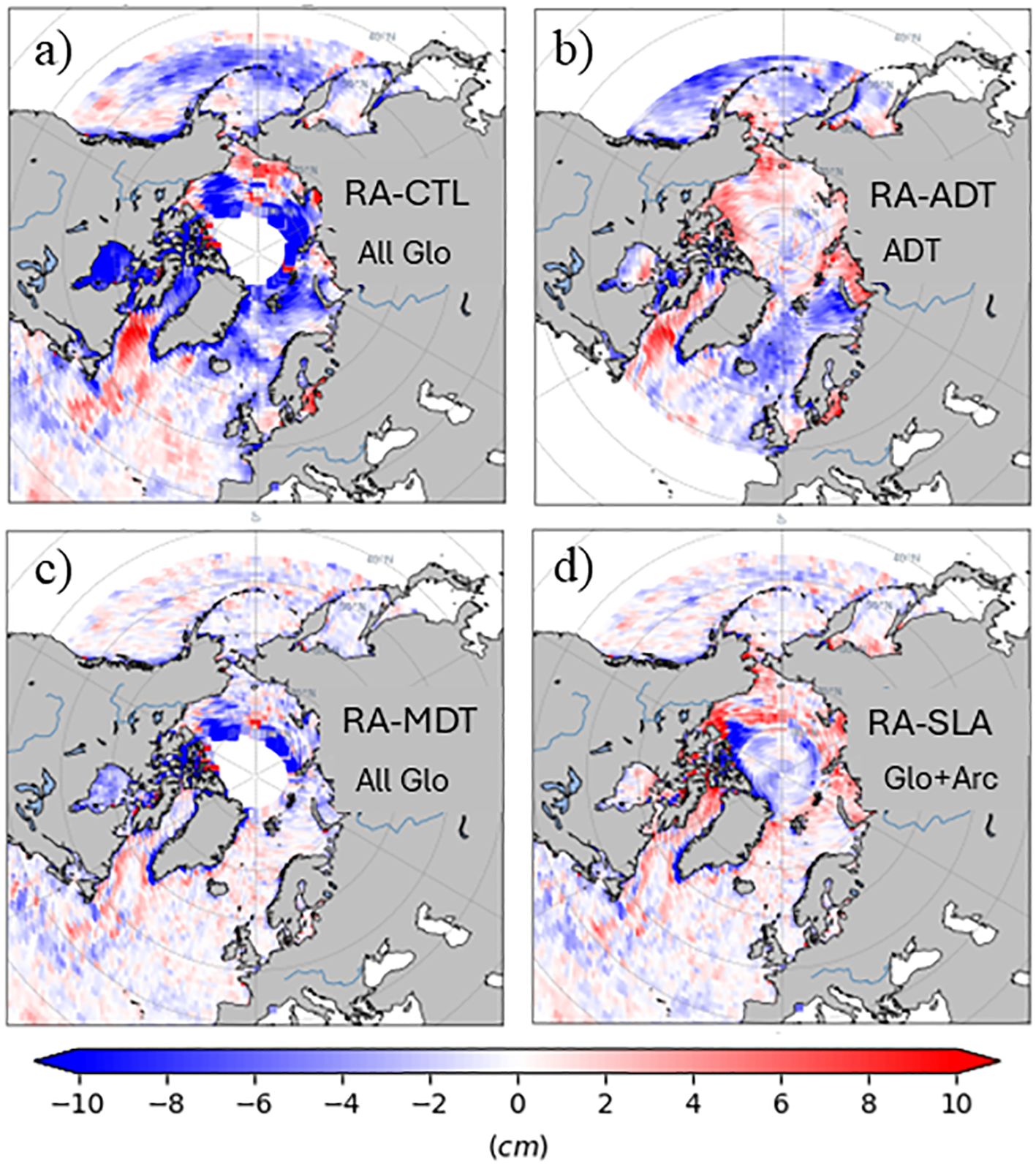
Figure 7 Mean innovations with respect to satellite altimetry for RA-CTL (A), RA-ADT (B), RA-MDT (C) and RA-SLA (D). Note that innovations represent differences with respect to the particular observations assimilated in each experiment. For RA-CTL and RA-MDT this includes global altimetry data (i.e. excluding ice covered areas) for Saral/Altika, Jason3, Sentinel3a, Sentinel3b and Cryosat2. Innovations for RA-SLA include both global and Arctic (leads) retrievals of SLA. Innovations for RA-ADT are with respect to the direct ADT fields that include both global and Arctic (leads) retrievals.

We can interpret these results as follows: In RA-CTL, an incoherence between the observation-based MDT product used and the effective model MDT results in excessively large mean innovations (i.e. greater than 10 cm) that inhibit the assimilation system from adequately correcting errors due to biased error statistics. By removing the mean difference in large-scale SLA in RA-MDT, it allows the data assimilation to properly assess (and correct) mesoscale features, but it prevents the system from correcting the basin-scale signals. In contrast, RA-ADT is allowed to adjust to the basin scale sea level present in the direct ADT product and to follow their variations on sub-seasonal, seasonal and longer timescales. As RA-SLA includes an additional dataset with respect to RA-MDT, it shows somewhat larger mean innovations, although still much smaller than RA-CTL. It would be possible in principle to iteratively correct these by removing the mean large-scale innovations from the MDT and producing an additional simulation. Note that since both RA-CTL and RA-MDT use the same observation errors (with larger values at higher latitudes), the larger mean innovations in RA-CTL (which are not present in RA-MDT) cannot be explained in terms of the observation error applied.

As SAM2 is a multi-variate assimilation system, it is important to assess how the change in one observational dataset affects other fields. As salinity has a more significant impact on density in colder waters, there should be a strong correlation between innovations of dynamic height (affected by satellite altimetry) and salinity. Mean innovations from salinity profiles (Figures 8, 9) show a clear reduction for all experiments in the overly saline bias (negative innovations) present in the North Sea and Norwegian coast as well as the overly fresh bias (positive innovations) in the Labrador Sea. These biases are significantly reduced in RA-MDT and RA-SLA suggesting a link to the representation of coastal features in the MDT. RA-ADT also shows some improvement in the North Sea and Norwegian Coast to a lesser degree, but shows some degradation in the Labrador Sea.

Figure 8

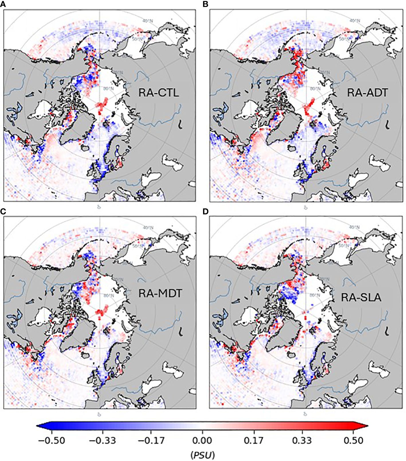
Figure 8 Mean innovations for salinity profile observations (psu) over the upper 500 m for RA-CTL (A), RA-ADT (B), RA-MDT (C) and RA-SLA (D).

Figure 9

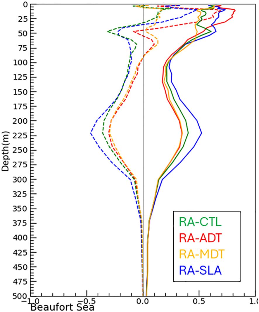
Figure 9 Innovation statistics for salinity profile observations (psu) over the Beaufort Sea region (shown in Figure 1) over the upper 500m. Mean (dashed line) and RMS (solid line) differences for RA-CTL (green), RA-ADT (red), RA-MDT (orange) and RA-SLA (blue) are shown.

There are also notable differences in the mean salinity innovations in the Beaufort Gyre. These biases show a high degree of spatial and temporal heterogeneity and may be affected by inadequate sampling due to the low number of in situ profiles. Nonetheless, we can see a reduction in both mean and RMS innovations of salinity between 100-350 m for RA-ADT and RA-MDT as compared to RA-CTL implying a positive benefit from the assimilation of satellite altimetry. Conversely, RA-SLA shows a significant degradation as compared to RA-MDT. The opposing impact of direct ADT versus SLA from leads suggests that the assimilation of altimetry from leads in ice covered waters is strongly sensitive to differences in MDT. Note that there is a marked degradation of RA-ADT in the upper 50 m not found in the other experiments.

Temperature profiles also show a small impact in the Bering Strait, Beaufort Sea, CAA and Central Arctic regions (not shown). Innovations for SST are equivalent for the four reanalyses (not shown).

5.2 Circulation and volume transports

The mean sea level innovations shown in Figure 7 suggest a basin-scale impact on sea level and circulation. Indeed, there is a significant modification of the mean SSH in RA-ADT as compared to RA-CTL (Figure 10A). In particular, there is a higher SSH in and along the Canadian Arctic Archipelago (CAA), which implies stronger volume and freshwater transports through CAA straits. There is also an increased SSH in the eastern part of the Barents Sea Opening consistent with stronger northward inflow. An inflated Beaufort Gyre can also be inferred from Figure 10, with steeper east-west gradients. Finally, significant changes near the North Pole and in Fram Strait suggest changes to the Transpolar Drift.

Figure 10

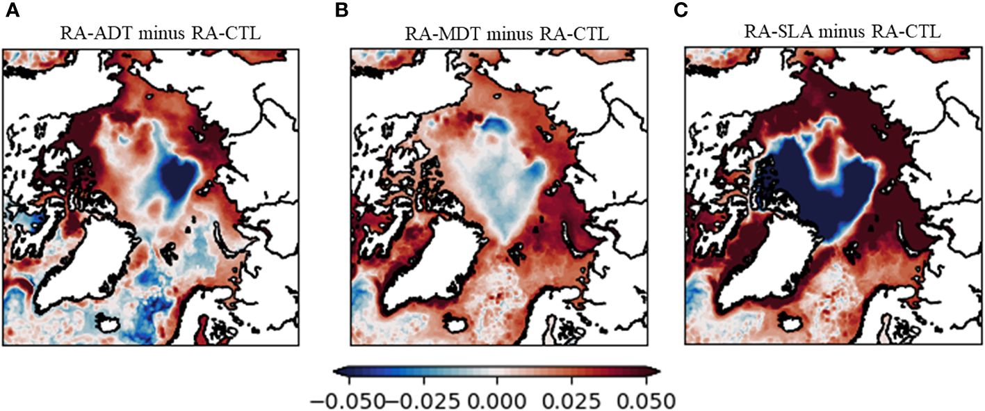
Figure 10 Difference in mean SSH (m) as compared to RA-CTL for RA-ADT (A), RA-MDT (B) and RA-SLA (C).

These differences are qualitatively similar to the pattern of differences found for RA-MDT and RA-SLA. That is, there is a general increase in SSH in Arctic shelf regions and a decrease in the central Arctic Ocean. This lower SSH is quite pronounced in RA-SLA creating sharp gradients along the shelf break. There is also a notable difference present in RA-ADT (but not in the other experiments) showing a lower SSH offshore in the Norwegian Sea. This implies a stronger onshore gradient of SSH and thus an impact on the Norwegian Current and transports into the Barents Sea (shown below).

The spatial pattern of mean currents is shown in Figure 11. Here we can clearly see an impact on the structure of the Beaufort Gyre in RA-ADT, with a reduction north of the CAA and intensification along the Alaskan coast. Conversely, RA-SLA shows an intensification north of the CAA. While all experiments show an impact on the Beaufort Gyre, the impact in RA-SLA is quite pronounced.

Figure 11

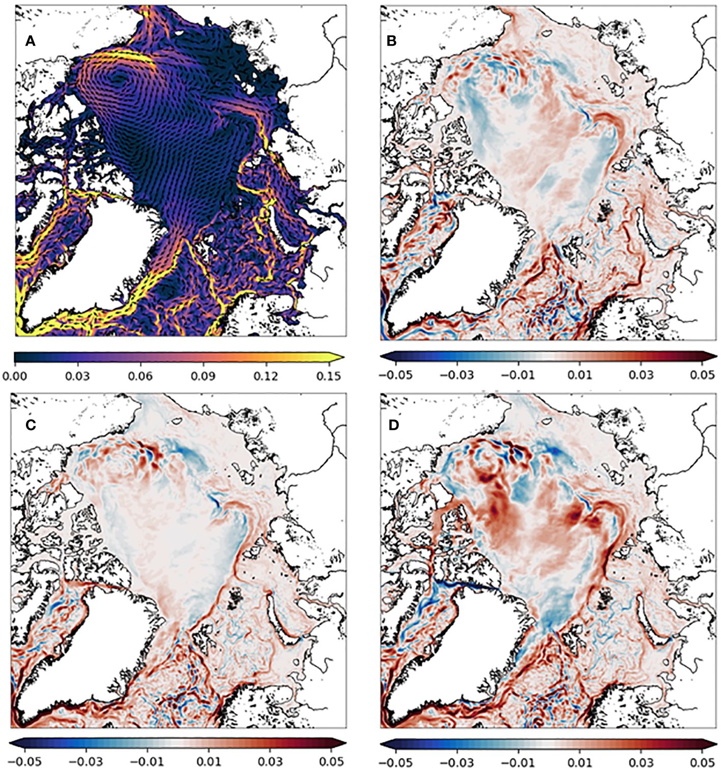
Figure 11 Mean surface currents (m/s) in RA-CTL (A) and differences (with respect to RA-CTL) for RA-ADT (B), RA-MDT (C) and RA-SLA (D).

There are also important impacts near the North Pole and in the Transpolar Drift, with an important intensification found in RA-ADT and RA-SLA. Smaller-scale impacts are also present in Fram Strait, along the Laptev Sea shelf break and near the Barents Sea Opening in all experiments.

To quantify these changes in circulation, we now present the impact of changes in circulation on transports through key Arctic gateways: Bering Strait, Barrow and Jones Straits, Nares Strait, Fram Strait, Davis Strait and the Barents Sea Opening (Table 3). Overall, we can see an opposite response in the net volume exchanges with the Arctic Ocean in RA-ADT as compared to RA-MDT and RA-SLA. RA-ADT shows a significant increase in volume transport through the CAA, with a 20% increase through Barrow and Jones Straits (combined), 8.8% through Nares Strait and 13% through Davis Strait. This increased Arctic export is compensated for by an increased inflow through the Barents Sea Opening (+0.17 Sv) and Bering Strait (+0.02 Sv). While Fram Strait shows very little change in total volume transport, a significant intensification of northward and southward flows through the strait are found (+1.1 Sv). These increased exchanges between the Atlantic and Arctic Oceans may have repercussions for the drift of plastics and other contaminants (see companion paper by Morales Maqueda et al., in prep.).

Table 3

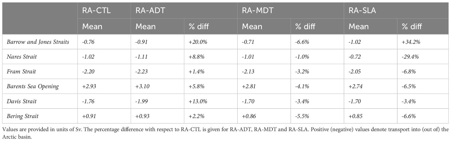
Table 3 Mean volume transports across key Arctic gateways.

Conversely, both RA-MDT and RA-SLA show a general decrease in net volume transport between the Arctic and North Atlantic. For Nares Strait, Fram Strait, the Barents Sea Opening and Bering Strait there is a reduced mean volume transport for RA-MDT, with an amplified response in RA-SLA. Barrow and Jones Straits show a somewhat different behavior with reduced transport for RA-MDT but an increased transport for RA-SLA. Davis Strait shows a slightly reduced transport for both RA-MDT and RA-SLA. These differences can be explained by the significant differences in mean SSH (Figure 10) with RA-MDT and RA-SLA showing higher SSH in Baffin Bay, whereas only RA-SLA shows an increase in SSH through the CAA and along the Alaskan coast.

Note that changes in total volume transport across a section are not necessarily reflected in mean surface currents (Figure 11) as important differences between surface and sub-surface currents exist in several locations (not shown). Additionally, important lateral differences are present across both Fram Strait and the Barents Sea Opening. For the latter, all experiments show an increase in the Norwegian Current. In RA-MDT and RA-SLA this is compensated for by a reduction in Atlantic inflow across the western half of the strait, whereas RA-ADT shows an increase (not shown).

Various monitoring efforts have been deployed across the key Arctic gateways and provide an estimate of heat, mass and freshwater transports. These estimates are often accompanied by significant error bars as total transports are estimated from a limited number of mooring observations. Moreover, these estimates are often only available for years outside the period of study. Nonetheless, the results here have been compared against observational estimates (e.g. Uotila et al. (2019) and references therein) and show that the RA-CTL and RA-ADT fall within reasonable estimates of volume transports. Given the large interannual variability and observational uncertainty it is difficult to discern if the intensification in Atlantic-Arctic exchange found in RA-ADT is closer to observed values. As a result, it is necessary to turn to indirect evidence to assess the impact of these changes in circulation.

5.3 Sea ice drift

As noted in the previous section, it is difficult to evaluate changes in ocean circulation due to a lack of available observations. However, circulation changes may affect the transfer of momentum to sea ice and thus be detectable in terms of sea ice drift and other features. Figure 12 shows maps of mean sea ice drift over the period Sep. 2018 to Mar. 2019 from the Ocean and Sea Ice Satellite Application Facility (OSI-SAF) product (Lavergne, 2016; Dybkjaer, 2018) together with fields from the different reanalyses evaluated here.

Figure 12

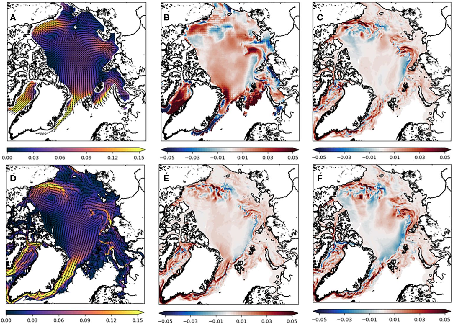
Figure 12 Mean sea ice drift speed (m/s) over the period Sep. 2018 to Mar. 2019 for OSI-SAF (A) and RA-CTL (D). Differences with respect to RA-CTL are shown for OSISAF (B), RA-ADT (C), RA-MDT (E) and RA-SLA (F).

The general pattern of sea ice drift is well reproduced in RA-CTL (Figure 12D) with a clear Beaufort Gyre and Transpolar Drift. Note that the OSI-SAF product has a lower spatial resolution than RIOPS and thus a direct comparison is not possible. As a result, it is not surprising to see several narrow areas of strong drift in the reanalyses represented as broader flows in OSI-SAF (e.g. Baffin Bay, Laptev Sea shelf break). Additionally, a larger uncertainty is present in the OSI-SAF product near the ice edge and thus differences in these regions should be interpreted with caution (e.g. East Greenland Current and Barents Sea; Wang et al., 2022). Nonetheless, the large-scale differences between OSI-SAF and RA-CTL shown in Figure 12B can be used as a general guide to assess the response in ice drift from the different experiments.

Indeed, we can see many similarities in differences between OSI-SAF and RA-CTL (Figure 12B) with what is found for the different experiments (Figures 12C, E, F). For example, the intensification along the Alaskan Coast and the broad intensification of the Transpolar Drift are consistent. The intensification of the ice drift along the Laptev Sea shelf break in RA-ADT and RA-SLA are also both in agreement with OSI-SAF. There is also a reduced drift speed present to varying extents along the shelf break north of the Barents and Kara Seas. This area of reduced drift implies an offshore displacement of the Transpolar Drift. Interestingly, the offshore displacement of the transpolar drift in RA-ADT appears consistent with OSI-SAF estimates. This displacement is amplified further in RA-SLA. However, with respect to that found in OSI-SAF it appears to be somewhat exaggerated with reduced ice drift extending from Fram Strait to the Laptev Sea. These results suggest that the impact of assimilation of direct ADT on surface currents is positive in general, whereas impacts for assimilation of SLA under ice may induce some areas of significant degradation.

5.4 Sea ice concentration increments

As noted in Section 4.1, the ocean analyses produced with SAM2 are blended with a 3DVar total ice concentration increment (by “total” we mean here the sum of ice concentration for all 10 ice thickness categories). Background error is not considered in this blending algorithm and thus the total ice concentration increment is very similar to the total ice concentration innovation. This is true everywhere except when the 3DVar ice analysis error exceeds a particular threshold and for regions where the ice concentration in either the model or analysis exceeds 90% or is less than 10%.

This blending is done at the end of each 7-day analysis window. As such, the total ice concentration increments can be considered as being approximately equivalent to 7-day forecast errors. As such, mean increments provide an indication of how well the model can simulate the evolution of the ice fields. Errors in total concentration due to formation/melt, advection or deformation will result in larger increments.

Figure 13 shows the mean total ice concentration increments for the four reanalyses for the summer (July, August, and September) season. While the mean total increments are quite similar, RA-SLA has an enhanced positive feature just north of the Kara Sea (north of 80°N between 60°E-120°E). This is consistent with the analysis presented in the previous sections that showed exaggerated changes to SSH, surface currents and ice drift in this area. The increase of ice increments is an additional indication that these changes do in fact represent a degradation. Differences in mean total ice concentration increments for the other seasons are relatively minor (not shown).

Figure 13

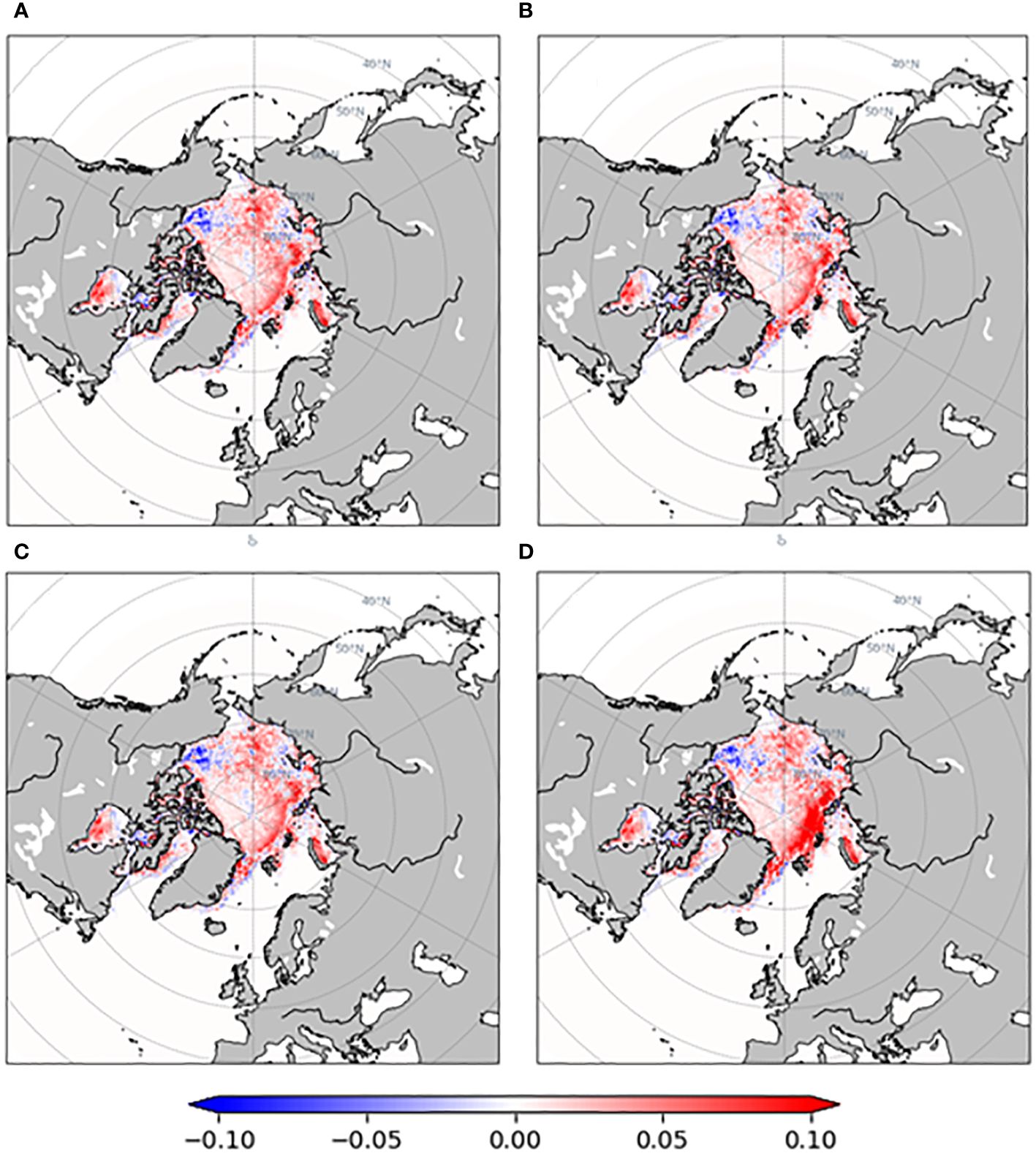
Figure 13 Mean total sea ice concentration increment (%) for RA-CTL (A), RA-ADT (B), RA-MDT (C) and RA-SLA (D).

5.5 Tide-gauge observations

To provide an additional independent comparison, the reanalyses are compared with tide-gauge observations from Prudhoe Bay station. Reanalysis values are first de-tided using values from the online harmonic analysis used in SAM2 (Smith et al., 2021). Inverse barometer effects from atmospheric pressure are also removed. Finally, the dynamic atmospheric correction used in the processing of satellite altimetry data is removed from both the observations and reanalyses. The resulting timeseries of sea level shows that the reanalyses provide an excellent reconstruction of the sea level variability, with correlations of about 0.9 (not shown). The differences in assimilation between the three experiments has a relatively minor impact on the sea level at Prudhoe Bay, with several periods of slightly improved (e.g. summer 2018) or degraded (e.g. fall 2017) sea level.

6 Summary and conclusions

Arctic ADT fields were successfully computed using the direct method (Equation 2) without using an MSS that may be of lower quality in the seasonally ice-covered region. The GOCO05c geoid was used as it was found to reduce the amplitude of small-scale spurious features due to inconsistencies with the altimetric measurements. However, some unphysical patterns remain in direct ADT fields for latitude over 83.5°N where GOCE satellite observations are not assimilated in the geoid. OI parameters for the mapping are tuned to consider geoid resolutions and the resulting direct ADT fields have reduced variance at spatial scales less than 200 km than classical ADT fields. Correlation with sea level tide gauge at Prudhoe Bay is similar between direct ADT and classical ADT fields.

The RIOPS operational ocean analysis system was modified to assimilate direct ADT (in place of SLA) and a four-year reanalysis was produced. Particular system modifications were required to adapt the system for assimilation of altimetry under ice as well as to accommodate the change in spatial scales present in the direct ADT product. The background error modes used in SAM2 to specify model error had an additional 100 passes of a Shapiro filter applied in order to reduce the variance below length scales of about 200 km, in accordance with spectral analyses of the direct ADT product. The resulting reanalysis (RA-ADT) was evaluated as compared to a control reanalysis equivalent to the operational version 2.2 of RIOPS (RA-CTL) in terms of mean innovations, circulation and volume transports across key Arctic gateways, sea ice drift and increments, and tide-gauge observations.

RA-ADT is found to provide reduced mean innovations suggesting a more balanced analysis. Significant changes in the sea surface height and surface currents are also found, indicating that the assimilation of direct ADT fields has a notable impact on the Arctic Ocean circulation and sea ice drift. Improvements in salinities are found along the Norwegian Coast with an intensification of the Norwegian Current. An intensification of Atlantic Water inflow and penetration is found, with stronger flow along the shelf break north of the Barents, Kara and Laptev Seas. This intensification appears to have a positive effect on surface ice drift. Investigation of volume transports through key Arctic gateways reveals that assimilation of direct ADT leads to an intensification of exchanges between the North Atlantic Ocean and the Arctic Ocean, with potential impacts on the simulated drift of contaminants in the Arctic.

While the assimilation of direct ADT fields appears to have positive impacts on circulation features in the Arctic, it is not clear the extent to which this is due to the assimilation of direct ADT itself (i.e. without use of an MDT as shown in Equation 2), as opposed to the addition of satellite altimetry from leads. This impact is assessed using two additional reanalyses: RA-MDT, with a modified MDT to reduce SLA innovations from global SLA data; and RA-SLA, that uses this new MDT together with SLA observations in leads (Prandi et al., 2021). Many of the impacts found for RA-ADT are also seen in RA-MDT. These include reduced mean innovations for sea level and salinity, and improvements in ice drift in the Beaufort Gyre and Transpolar Drift (and associated surface currents).

The addition of SLA from leads in the sea ice appears to produce a degradation in a number of features. Larger innovations of sea level are found together with a degradation of salinity innovations in the Beaufort Sea. These changes appear to lead to a reduction in volume transports across the key Arctic gateways. A strong intensification of the surface currents is found north of the Barents and Kara Sea that leads to reduced sea ice drift. This implies an effective offshore displacement of the Transpolar Drift inconsistent with observed estimates from OSI-SAF. Additionally, larger increments in sea ice concentration are found suggesting the change in ice drift when assimilating SLA from leads represents a degradation. These results suggest that the reduced exchange between the Arctic and Atlantic Oceans when assimilating SLA from leads may also represent a degradation.

Several conclusions can be drawn from these results. First, assimilation of satellite altimetry retrievals from leads can have a positive impact on water mass properties and circulation in the Arctic Ocean. It is tempting to also conclude from these results that assimilation of direct ADT is more beneficial than assimilating SLA from leads, as the latter was found to produce questionable changes in surface currents and volume transports. However, the results from RA-MDT highlight the strong sensitivity of SLA assimilation to the choice of MDT. Indeed, many of the improvements seen with the assimilation of direct ADT were also found with the modified MDT only. As such, if the MDT was further corrected using mean innovations from RA-SLA, it may be possible to obtain more consistent results assimilating SLA from leads.

This study highlights the large uncertainties that exist in present operational ocean forecasting systems for the Arctic Ocean due to the relative paucity and reduced quality of observations compared to ice-free areas of the world’s oceans. Extension of gravity data to cover the north pole is required to provide a truly pan-Arctic direct ADT that would allow an accurate assessment of Arctic transports. Moreover, this study underscores the need for dedicated and focused efforts to address this critical gap in the Global Ocean Observing System.

Data availability statement

The raw data supporting the conclusions of this article will be made available by the authors, without undue reservation. SLA and profile data used in this study was provided by the EU Copernicus Marine Environmental Monitoring Service. Argo profile data were collected and made freely available by the International Argo Program and the national programs that contribute to it. (https://argo.ucsd.edu, https://www.ocean-ops.org). The Argo Program is part of the Global Ocean Observing System.

Author contributions

GS: Conceptualization, Funding acquisition, Investigation, Methodology, Project administration, Software, Supervision, Validation, Writing – original draft, Writing – review & editing. CH-P: Investigation, Software, Validation, Visualization, Writing – review & editing. A-AG: Investigation, Software, Supervision, Validation, Visualization, Writing – review & editing. FR: Investigation, Software, Validation, Visualization, Writing – review & editing. KP: Investigation, Methodology, Software, Supervision, Validation, Visualization, Writing – review & editing. PV: Conceptualization, Investigation, Methodology, Software, Validation, Visualization, Writing – review & editing. YF: Investigation, Methodology, Project administration, Supervision, Validation, Writing – review & editing. SM: Conceptualization, Funding acquisition, Methodology, Project administration, Supervision, Writing – review & editing. MM: Conceptualization, Funding acquisition, Investigation, Methodology, Project administration, Validation, Writing – review & editing.

Funding

The author(s) declare financial support was received for the research, authorship, and/or publication of this article. This work was funded by European Space Agency project Clean Arctic (Contract No. 4000137958/22/I-DTlr). GS, FR, KP, and A-AG were supported by Government of Canada in-kind contributions to project Clean Arctic.

Acknowledgments

We would like to thank ESA for financing this project and M.H. Rio for her helpful suggestions throughout the project. We would also like to thank D. Surcel Colan for her support. F. Dupont provided useful suggestions with regards to impacts on transports. Y. Liu provided assistance with scripts to filter the background error modes. We would also like to thank colleagues at Mercator Ocean International for their assistance and support of the SAM2 code. Two reviewers provided helpful suggestions and comments that improved the manuscript.

Conflict of interest

Authors PV, YF, and SM were employed by company Collecte Localisation Satellites.

The remaining authors declare that the research was conducted in the absence of any commercial or financial relationships that could be construed as a potential conflict of interest.

Publisher’s note

All claims expressed in this article are solely those of the authors and do not necessarily represent those of their affiliated organizations, or those of the publisher, the editors and the reviewers. Any product that may be evaluated in this article, or claim that may be made by its manufacturer, is not guaranteed or endorsed by the publisher.

References

Abdalla S., Kolahchi A. A., Ablain M., Adusumilli S., Bhowmick S. A., Alou-Font E., et al. (2021). Altimetry for the future: Building on 25 years of progress. Adv. Space Res. 68, 319–363. doi: 10.1016/j.asr.2021.01.022

CrossRef Full Text | Google Scholar

Androsov A., Nerger L., Schnur R., Schröter J., Albertella A., Rummel R., et al. (2019). On the assimilation of absolute geodetic dynamic topography in a global ocean model: impact on the deep ocean state. J. Geodesy 93, 141–157. doi: 10.1007/s00190-018-1151-1

CrossRef Full Text | Google Scholar

Armitage T. W. K., Bacon S., Ridout A. L., Thomas S. F., Aksenov Y., Wingham D. J. (2016). Arctic sea surface height variability and change from satellite radar altimetry and GRACE 2003–2014. J. Geophys. Res. - Oceans 121, 4303–4322. doi: 10.1002/2015JC011579

CrossRef Full Text | Google Scholar

Benkiran M., Greiner E. (2008). Impact of the incremental analysis updates on a real-time system of the North Atlantic Ocean. J. Atm. Oc. Tech. 25, 2055–2073. doi: 10.1175/1520-0493(1996)124<1256:DAUIAU>2.0.CO;2

CrossRef Full Text | Google Scholar

Benkiran M., Ruggiero G., Greiner E., Le Traon P. Y., Rémy E., Lellouche J. M., et al. (2021). Assessing the impact of the assimilation of swot observations in a global high-resolution analysis and forecasting system part 1: Methods. Front. Mar. Sci. 8, 691955. doi: 10.3389/fmars.2021.691955

CrossRef Full Text | Google Scholar

Bloom S. C., Takacs L. L., Da Silva A. M., Ledvina D. (1996). Data assimilation using incremental analysis updates. Mon. Wea. Rev. 124, 1256–1271. doi: 10.1175/1520-0493(1996)1242.0.CO;2

CrossRef Full Text | Google Scholar

Brasnett B., Colan D. S. (2016). Assimilating retrievals of sea surface temperature from VIIRS and AMSR2. J. Atm. Oc. Tech. 33, 361–375. doi: 10.1175/JTECH-D-15-0093.1

CrossRef Full Text | Google Scholar

Bretherton F. P., Davis R. E., Fandry C. (1976). A technique for objective analysis and design of oceanographic experiments applied to MODE-73. Deep-Sea Res. Oceanogr. Abs. 23, 559–582. doi: 10.1016/0011-7471(76)90001-2

CrossRef Full Text | Google Scholar

Bruinsma S. L., Förste C., Abrikosov O., Lemoine J., Marty J., Mulet S., et al. (2014). ESA’s satellite-only gravity field model via the direct approach based on all GOCE data. Geophys. Res. Lett. 41, 7508–7514. doi: 10.1002/2014GL062045

CrossRef Full Text | Google Scholar

Buehner M., Caya A., Carrieres T., Pogson L. (2016). Assimilation of SSMIS and ASCAT data and the replacement of highly uncertain estimates in the Environment Canada Regional Ice Prediction System. Q. J. R. Met. Soc 142, 562–573. doi: 10.1002/qj.2408

CrossRef Full Text | Google Scholar

Buehner M., Caya A., Pogson L., Carrieres T., Pestieau P. (2013). A new environment Canada regional ice analysis system. Atmos.-Ocean 51, 18–34. doi: 10.1080/07055900.2012.747171

CrossRef Full Text | Google Scholar

Caldwell P. C., Merrifield M. A., Thompson P. R. (2015). Sea level measured by tide gauges from global oceans — the Joint Archive for Sea Level holdings (NCEI Accession 0019568), Version 5.5 (Hawaii, USA: NOAA National Centers for Environmental Information, Dataset). doi: 10.7289/V5V40S7W

CrossRef Full Text | Google Scholar

Chikhar K., Lemieux J. F., Dupont F., Roy F., Smith G. C., Brady M., et al. (2019). Sensitivity of Ice Drift to Form Drag and Ice Strength Parameterization in a Coupled Ice–Ocean Model. Atmos.-Ocean 57 (5), 329–349. doi: 10.1080/07055900.2019.1694859

CrossRef Full Text | Google Scholar

Dupont F., Higginson S., Bourdallé-Badie R., Lu Y., Roy F., Smith G. C., et al. (2015). A high-resolution ocean and sea-ice modelling system for the Arctic and North Atlantic Oceans. Geosci. Model. Dev. 8, 1577–1594. doi: 10.5194/gmd-8-1577-2015

CrossRef Full Text | Google Scholar

Dybkjaer G. (2018) Medium Resolution Sea Ice Drift Product User Manual; Version 2.0 (The Ocean and Sea Ice Satellite Application Facility (OSI SAF). Available online at: https://osisaf-hl.met.no/sites/osisaf-hl/files/user_manuals/osisaf_ss2_pum_sea-ice-drift-mr_v2p0.pdf (Accessed 7 February 2024).

Google Scholar

Fecher T., Pail R., Gruber T. (2017). GOCO05c: A new combined gravity field model based on full normal equations and regionally varying weighting. Surveys Geophysics 38, 571–590. doi: 10.1007/s10712-016-9406-y

CrossRef Full Text | Google Scholar

Förste C., Bruinsma, Sean L., Abrikosov O., Lemoine J.-M., Marty J. C., Flechtner F., et al. (2014). EIGEN-6C4 The latest combined global gravity field model including GOCE data up to degree and order 2190 of GFZ Potsdam and GRGS Toulouse (Potsdam, Germany: GFZ Data Services). doi: 10.5880/ICGEM.2015.1

CrossRef Full Text | Google Scholar

Hunke E. C. (2001). Viscous-plastic sea ice dynamics with the EVP model: linearization issues. J. Comput. Phys. 170, 18–38. doi: 10.1006/jcph.2001.6710

CrossRef Full Text | Google Scholar

Hunke E. C., Lipscomb W. H. (2008). CICE: The Los Alamos sea ice model. Documentation and software user’s manual version 4.0 (Tech. Rep. LA-CC-06-012) (Los Alamos, NM: Los Alamos National Laboratory).

Google Scholar

Jacobs G. A., D’Addezio J. M., Bartels B., Spence P. L. (2021). Constrained scales in ocean forecasting. Adv. Space Res. 68, 746–761. doi: 10.1016/j.asr.2019.09.018

CrossRef Full Text | Google Scholar

Kvas A., Brockmann J. M., Krauss S., Schubert T., Gruber T., Meyer U., et al. (2021). GOCO06s – a satellite-only global gravity field model. Earth System Sci. Data 13, 99–118. doi: 10.5194/essd-13-99-2021

CrossRef Full Text | Google Scholar

Lavergne T. (2016) Low Resolution Sea Ice Drift. Product User’s Manual; Version 1.8 (The Ocean and Sea Ice Satellite Application Facility (OSI SAF). Available online at: https://osisaf-hl.met.no/sites/osisaf-hl.met.no/files/user_manuals/osisaf_cdop2_ss2_pum_sea-ice-drift-lr_v1p8.pdf (Accessed 7 February 2024).

Google Scholar

Lellouche J. M., Greiner E., Le Galloudec O., Garric G., Regnier C., Drevillon M., et al. (2018). Recent updates to the Copernicus Marine Service global ocean monitoring and forecasting real-time 1/12° high-resolution system. Ocean Sci. 14, 1093–1126. doi: 10.5194/os-14-1093-2018

CrossRef Full Text | Google Scholar

Lellouche J. M., Le Galloudec O., Drévillon M., Régnier C., Greiner E., Garric G., et al. (2013). Evaluation of global monitoring and forecasting systems at Mercator Océan. Ocean Sci. 9, 57. doi: 10.5194/os-9-57-2013

CrossRef Full Text | Google Scholar

Le Traon P. Y., Antoine D., Bentamy A., Bonekamp H., Breivik L. A., Chapron B., et al. (2015). Use of satellite observations for operational oceanography: recent achievements and future prospects. J. Oper. Ocean 8, s12–s27. doi: 10.1080/1755876X.2015.1022050

CrossRef Full Text | Google Scholar

Lipscomb W. H., Hunke E. C., Maslowski W., Jakacki J. (2007). Ridging, strength, and stability in high-resolution sea ice models. J. Geophys. Res. 112. doi: 10.1029/2005JC003355

CrossRef Full Text | Google Scholar

Madec G., Bourdallé-Badie R., Chanut J., Clementi E., Coward A., Ethé C., et al. (2019). NEMO ocean engine. In Notes du Pôle de modélisation de l’Institut Pierre-Simon Laplace (IPSL) (v4.0, Number 27) (Paris, France: Zenodo). doi: 10.5281/zenodo.3878122

CrossRef Full Text | Google Scholar

Müller F. L., Wekerle C., Dettmering D., Passaro M., Bosch W., Seitz F. (2019). Dynamic ocean topography of the northern Nordic seas: a comparison between satellite altimetry and ocean modeling. Cryosphere 13, 611–626. doi: 10.5194/tc-13-611-2019

CrossRef Full Text | Google Scholar

Pail R., Bruinsma S., Migliaccio F., Förste C., Goiginger H., Schuh W. D., et al. (2011). First GOCE gravity field models derived by three different approaches. J. Geodesy 85, 819–843. doi: 10.1007/s00190-011-0467-x

CrossRef Full Text | Google Scholar

Pavlis N. K., Holmes S. A., Kenyon S. C., Factor J. K. (2012). The development and evaluation of the earth gravitational model 2008 (egm2008). J. Geophys. Res. – Solid Earth 117. doi: 10.1029/2011JB008916

CrossRef Full Text | Google Scholar

Prandi P., Poisson J.-C., Faugère Y., Guillot A., Dibarboure G. (2021). Arctic sea surface height maps from multi-altimeter combination. Earth Syst. Sci. Data 13, 5469–5482. doi: 10.5194/essd-13-5469-2021

CrossRef Full Text | Google Scholar

Pujol M.-I., Schaeffer P., Faugère Y., Raynal M., Dibarboure G., Picot N. (2018). Gauging the improvement of recent mean sea surface models: A new approach for identifying and quantifying their errors. J. Geophys. Res.-Oceans 123, 5889–5911. doi: 10.1029/2017JC013503

CrossRef Full Text | Google Scholar

Rio M.-H., Mulet S., Picot N. (2014). Beyond GOCE for the ocean circulation estimate: Synergetic use of altimetry, gravimetry, and in situ data provides new insight into geostrophic and Ekman currents. Geophys. Res. Lett. 41, 8918–8925. doi: 10.1002/2014GL061773

CrossRef Full Text | Google Scholar

Roy F., Chevallier M., Smith G. C., Dupont F., Garric G., Lemieux J.-F., et al. (2015). Arctic sea ice and freshwater sensitivity to the treatment of the atmosphere-ice-ocean surface layer. J. Geophys. Res. - Oceans 120, 4392–4417. doi: 10.1002/2014JC010677

CrossRef Full Text | Google Scholar

Smith G. C., Fortin A. S. (2022). Verification of eddy properties in operational oceanographic analysis systems. Ocean Mod. 172, 101982. doi: 10.1016/j.ocemod.2022.101982

CrossRef Full Text | Google Scholar

Smith G. C., Liu Y., Benkiran M., Chikhar K., Surcel Colan D., Gauthier A. A., et al. (2021). The Regional Ice Ocean Prediction System v2: a pan-Canadian ocean analysis system using an online tidal harmonic analysis. Geosci. Model. Dev. 14, 1445–1467. doi: 10.5194/gmd-14-1445-2021

CrossRef Full Text | Google Scholar

Smith G. C., Roy F., Reszka M., Surcel Colan D., He Z., Deacu D., et al. (2016). Sea ice forecast verification in the Canadian global ice ocean prediction system. Q. J. R. Meteo. Soc 142, 659–671. doi: 10.1002/qj.2555

CrossRef Full Text | Google Scholar

Surcel Colan D., Dupont F., Gauthier A.-A., Islam M. R., Chikhar K., Hata Y., et al. (2021) Changes from version 2.1.0 to version 2.2.0 of the Regional Ice Ocean Prediction System (RIOPS). Canadian Centre for Meteorological and Environmental Prediction (CCMEP) Technical Report. Dec. 1, 2021. Available online at: https://collaboration.cmc.ec.gc.ca/cmc/cmoi/product_guide/docs/tech_notes/technote_riops-220_e.pdf.

Google Scholar

Tonani M., Balmaseda M., Bertino L., Blockley E., Brassington G., Davidson F., et al. (2015). Status and future of global and regional ocean prediction systems. J. Oper. Ocean 8, s201–s220. doi: 10.1080/1755876X.2015.1049892

CrossRef Full Text | Google Scholar

Uotila P., Goosse H., Haines K., Chevallier M., Barthélemy A., Bricaud C., et al. (2019). An assessment of ten ocean reanalyses in the polar regions. Clim. Dyn 52, 1613–1650. doi: 10.1007/s00382-018-4242-z

CrossRef Full Text | Google Scholar

Wang X., Chen R., Li C., Chen Z., Hui F., Cheng X. (2022). An intercomparison of satellite derived Arctic sea ice motion products. Rem. Sens. 14, 1261. doi: 10.3390/rs14051261

CrossRef Full Text | Google Scholar

Wong A. P., Wijffels S. E., Riser S. C., Pouliquen S., Hosoda S., Roemmich, et al. (2020). Argo data 1999–2019: two million temperature-salinity profiles and subsurface velocity observations from a global array of profiling floats. Front. Mar. Sci. 7. doi: 10.3389/fmars.2020.00700

CrossRef Full Text | Google Scholar

Xu M., Wang Y., Zhang J., Yang D., Yin X., Gao Y., et al. (2022). Data assimilation in a regional high-resolution ocean model by using Ensemble Adjustment Kalman Filter and its application during 2020 cold spell event over Asia-Pacific region. Appl. Ocean Res. 129, 103375. doi: 10.1016/j.apor.2022.103375

CrossRef Full Text | Google Scholar

Zingerle P., Brockmann J. M., Pail R., Gruber T., Willberg M. (2019). The polar extended gravity field model TIM_R6e (Potsdam, Germany: GFZ Data Services). doi: 10.5880/ICGEM.2019.005

CrossRef Full Text | Google Scholar