Seasonal and vertical tidal variability in the Southeastern Mediterranean Sea

Currents and pressure records from the DeepLev mooring station and drifter data in the eastern Levantine Basin were analyzed to identify the dominant tidal constituents and their seasonal and depth variability. Harmonic and spectral analysis of seasonal segments of currents and pressure reveal key attributes of the tidal regime: (1) dominant semidiurnal sea level variability; (2) seasonal variation of semidiurnal and diurnal tides in both currents and pressure datasets; and (3) significant diurnal currents with weak semidiurnal currents across all seasons. The most dominant tidal constituent from the pressure dataset is the M2 (12.4 h). Results from pressure datasets align with previous models and observations of semidiurnal tides. In contrast, the diurnal tides are larger than previously reported by 8—9 cm in the winter and 1—2 cm in the summer. The surface current tidal regime differs from prior reports in the eastern Levantine Basin, with M2 magnitudes weaker by 1 cm s^-1, while the diurnal tides (K1, O1) are 1—2 cm s^-1 larger. Seasonal segments showed seasonal differences in the local tidal regime’s amplitudes. The most pronounced seasonal differences were with the K1 and S2 tides, with differences between winter and fall of 7 cm for the K1 and 4 cm between summer and fall for the S2. We utilized the DeepLev datasets to compare a moored device with surface drifters near DeepLev by analyzing the M2 and S2 tides. Additionally, we examined data at different dataset lengths, considering the time constraints needed to resolve the tides adequately. Longer datasets improved the resolution of the tidal analysis and reduced amplitude leakages from nearby frequencies, resulting in a more realistic and accurate analysis of the tidal currents. Conversely, longer datasets resulted in fewer drifters remaining our study region for the allotted dataset length. From 32 available segments in 15 day dataset to 7 with a 30 day dataset, reducing the effectiveness of drifters as a local tidal research tool.

1 Introduction

Tidal currents and tidal variations in sea level have attracted scholars for over 2000 years (see review by Deparis et al., 2013). Understanding the tidal regime in microtidal regions, specifically in the eastern Mediterranean basin, is essential for numerical models. Studies have shown that tides indirectly influence Levantine Intermediate Water dispersal paths in the eastern basin (Sannino et al., 2015) and generate diurnal circulations near the Egyptian coast (Palma et al., 2020). While tides in the Mediterranean Sea have been studied before, only a few studies were conducted in the deep part of the Levantine Basin.

The Mediterranean is a semi-enclosed basin with a complex bathymetry connected to the Atlantic Ocean by the Straits of Gibraltar. The Sicily Channel divides it into two major basins—the western and the eastern—and each basin includes many shallow and deep subbasins (Albérola et al., 1995; Gasparini et al., 2004). Thus, the characteristics of the tides can vary across different regions and depths (Poulain et al., 2018).

Both observations and models have been used to study tides in different regions of the Mediterranean. Observations include current measurements from shipboard and high-frequency coastal radars in the western Mediterranean and Strait of Sicily (Garcia-Gorriz et al., 2003; Gasparini et al., 2004; Chavanne et al., 2007; Cosoli et al., 2015; Soto-Navarro et al., 2016), from moored instruments and surface drifters across the Mediterranean (Lafuente and Lucaya, 1994; Albérola et al., 1995; Poulain and Zambianchi, 2007; Ursella et al., 2014; Poulain et al., 2012; Poulain et al., 2013; Poulain and Centurioni, 2015; Poulain et al., 2018). In addition, numerical models with various complexities were also used to study tides in the entire Mediterranean Sea (e.g., Tsimplis et al., 1995; Arabelos et al., 2011). However, there is an observational gap in the deep waters of the eastern Levantine basin, with few moored deep and long-term datasets available to study offshore tides.

Drifter data has been used to estimate harmonic tidal constituents, both globally (Poulain and Centurioni, 2015) and regionally in macro and microtidal regions (Poulain et al., 2018; Lie et al., 2002; Ohshima et al., 2002) and to compare with tidal prediction models (Zaron and Elipot 2020; Kodaira et al. 2016; Zaron and Ray, 2017; Crawford et al., 1998). Using drifters for tidal current analysis has the benefit of inexpensive observations with short sampling intervals at a distance from the coast, where most of the moored devices are stationed.

A few previous studies identified four main constituents (M2, S2, K1, and O1) in models, drifters, and observations in the eastern Mediterranean and the Strait of Sicily (e.g., Tsimplis et al., 1995; Gasparini et al., 2004; Cosoli et al., 2015; Poulain et al., 2018). See Table 1 for the corresponding periods. Arabelos et al. (2011) identified and applied additional constituents in their numerical model. Differences in the dominant constituents at different locations are expected due to the complexity of the coastline and bathymetry.

Table 1

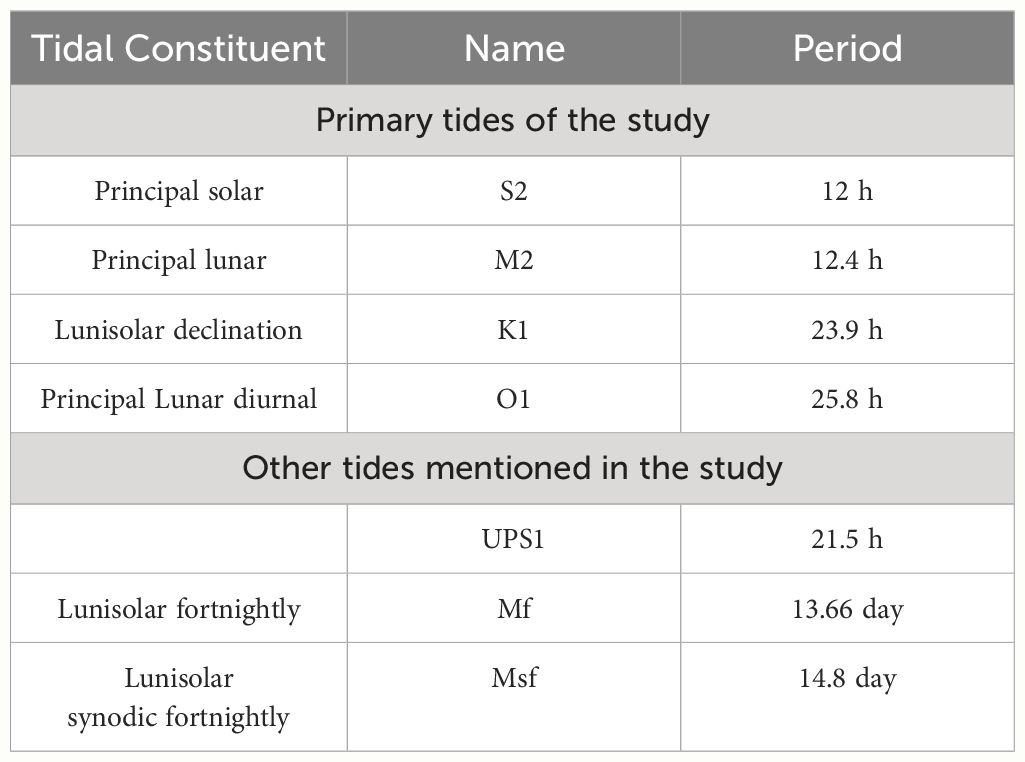
Table 1 Tidal constituents and their periods are either the primary focus or are mentioned in this paper.

Additional tidal constituents that were found in the tidal analysis include the diurnal UPS1 and the long fortnightly Mf and Msf, whose existence and importance in the eastern Mediterranean need to be clarified. Several observations at Alexandria have reported the presence of the UPS1 tide (El-Geziry and Radwan, 2012; El-Geziry, 2021; Khedr et al., 2018). Oscillations with a period similar to the UPS1 tide were also observed at the Strait of Otranto (Ursella et al., 2014) and the Adriatic Sea (Medvedev et al., 2020). However, Ursella et al. (2014) and Medvedev et al. (2020) attributed this to the 21.5 h fundamental eigenmode in the Adriatic. Studies at the Strait of Gibraltar identified the existence of the Mf and Msf constituents (Tsimplis and Bryden, 2000; Millot and Garcia-Lafuente, 2011; Sammartino et al., 2015). These frequencies have been attributed to nonlinear interactions between semidiurnal and diurnal tidal constituents in shallow seas and sea shelves (Kwong et al., 1997). However, the Mf and Msf constituents have also been observed in the Adriatic Sea (Chavanne et al., 2007; Vilibić et al., 2010) and the Marmara Sea (Ferrarin et al., 2018).

The seasonality of tides, and in particular, the seasonality of the M2 tide, has been studied both theoretically and experimentally. Müller et al. (2014) showed variations in the M2 tide in global models and tide gauge data from several areas worldwide, such as Victoria, Canada, and Cuxhaven, Germany. They attributed the effects of seasonal differences in stratification to the seasonality of the tides. They postulate that stronger stratification leads to less mixing and, hence, to less loss of kinetic energy of the barotropic tide to turbulence, resulting in tides with larger amplitudes. Wang et al. (2020) attempted to replicate the seasonality found in tide gauges in the Bohai Sea using a three-dimensional MITgcm model based on Müller’s study with limited results. Ray (2022) proposes several physical mechanisms underlying the seasonality of the M2 tide group. The first is climate-induced variations such as those found by Müller et al. (2014). Another is astronomical changes due to the Sun’s third body perturbations of the lunar orbit, which are small and finally compound tides such as the MSK2 tide. Ray (2022) used long-duration O(10 yrs) data sets taken from coastal regions in St. Malo (France), Chittagong (Bangladesh), and Port Orford (Oregon), which allowed the high-resolution spectral analysis necessary for such a study. Our study cannot capture the minor frequency differences in the M2 tidal group, and we shall refer to them as the same constituent.

Drifters in the eastern Levantine basin have also been used to study the tides in the region (Poulain et al., 2018). There are spatial and temporal limitations to using drifters for tidal analysis. Temporal constraints apply to the sampling frequency and period following signal analysis theory. More broadly, the confidence interval of the estimated values becomes narrower as the period increases (Bendat and Piersol, 2011). This phenomenon is experimentally shown in Lie et al. (2002), where longer drifter datasets resulted in less deviation from the known M2 and K1 harmonic constants in the Yellow Sea. As for spatial limitations, when a drifter is transported hundreds of kilometers meridionally, the inertial frequency it experiences can vary significantly. Work on the M2 tide by Carrère et al. (2004) shows that the M2’s amplitude is not stable in areas with ocean mesoscale activities and strong topographic features. The topography near the Israeli coast can vary significantly, further affecting the tide, as seen in Rosentraub and Brenner (2007) through multiple moored devices along the coast. Therefore, a dataset of the spatial order of 1°x1° is needed to minimize the variability of the results due to spatial changes while maintaining accurate tidal harmonic analysis and spectral analysis.

Here, we use long-term observations collected at the DeepLev mooring station in the Levantine Basin, referred to as “DeepLev” (Katz et al., 2020). The DeepLev dataset is the first of its kind in the eastern Mediterranean, enabling the examination of depth and seasonal changes in the pressure and currents in the region. The dataset allows novel research of the Levantine basin tides at different seasons and depths. Along with satellite-tracked surface drifters, we (1) identify the dominant tidal constituents in the Levantine Basin and compare the results with previous studies, (2) study the vertical and seasonal variability of the dominant constituents, (3) compare the tidal constituents derived from moored current meters to those derived from surface drifters, and (4) examining the effectiveness of the dataset length of drifters.

Our results from pressure observations near the Israeli coast demonstrate a dominant M2 tide constituent presence in every season and at all depths. In the current measurements, tidal analysis shows weak semidiurnal and diurnal tides at all depths, with a seasonal difference between 3 cm s^-1 in the fall and 0.9 cm s^-1 in the spring for the tidal constituent of K1 at 30 m. In general, seasonality variations are less pronounced with depth. We also compared the magnitudes of tidal constituents derived from surface drifters and moored instruments, demonstrating the difficulties associated with balancing the temporal length of the drifter’s trajectory and its meridional movement.

The paper’s structure is as follows: Section 2 describes the data used and analysis methods. Section 3 presents our results, and Section 4 discusses them.

2 Materials and methods

The physical properties of the water column in the Levantine basin were measured at the DeepLev mooring station (Figure 1) situated ~50 km offshore Haifa, Israel, (33◦ 03.67’ N; 34◦ 29.296’ E), where the water depth is ~1500 m (Katz et al., 2020). The instruments were deployed for 6—9 months, with gaps in the data between consecutive deployments and occasionally within the deployment periods. For simplicity, we converted pressure from decibar to m using a 1:1 ratio for all the analyses presented in this paper. The samples have been split by season, defined as winter (December—February), spring (March-May), summer (June—August), and autumn (September—November). A description of the exact durations is presented in Supplementary Table 1.

Figure 1

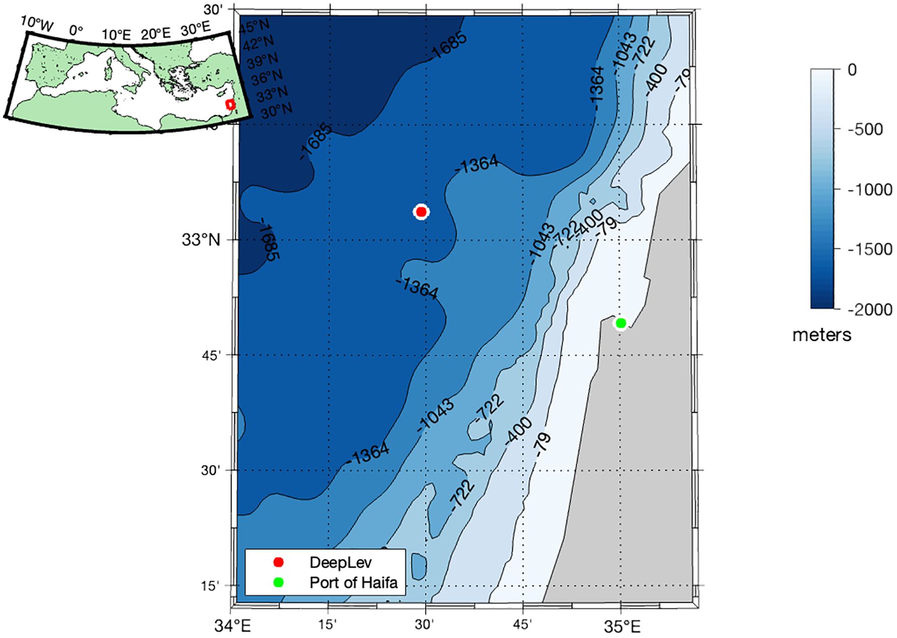
Figure 1 The map in the top left corner shows the Mediterranean Sea. The red box on the map shows the area of the larger map showing the location of the DeepLev mooring station (white full circle with a red dot), the location of the Port of Haifa (white circle with a red dot), with bathymetry contour color (Pawlowicz, 2020).

Currents were measured using Acoustic Doppler Current Profilers (ADCPs) employed at various depths. Three downward-looking Teledyne RDI ADCPs were used: a 300 kHz system at approximately 30 m, measuring from 30 m to 100 m in 2 m bins with ensembles every 15 min; a 150 kHz system at approximately 100 m, with 4 m bins measuring down to about 200 m depth, with ensembles every one h; and another 150 kHz system at approximately 400 m, measuring currents between 400—670 m in 10 m bins, with ensembles every two h. All Teledyne RDI ADCP data underwent post-processing quality control, including magnetic declination correction, using Teledyne RDI ADCP software. The following thresholds were used: Percentage Good Pings at 55%, Correlation Magnitude at 80, and Error Velocity at four cm s^-1. Incoming data that failed one or more of the tests were excluded. No correction for tilt or pressure was done. Two Nortek Aquadopp single point current meters were fixed at 1310 m and 1492 m, measuring temperature, pressure, and currents, creating ensembles every ½ h. No post-processing quality control was performed. Five discrete depths were chosen from the measurements to analyze the current at different depths: 30 m, 50 m, 70 m, 160 m, 400 m, and 1300 m.

Pressure variability was recorded by two RBR—CONCERTO CTDs placed at 90 m and 290 m depths, measuring at a time resolution of 10 min in the first deployment and one min in the following deployments. A SeaBird MicroCat CTD, placed at 185 m, was added to the array starting from the second deployment, measuring at a time resolution of 10 min throughout. CTD depths are noted as 90 m, 200 m, and 300 m. Additional pressure measurements were used from the Nortek Aquadopp at 1310 m, noted as 1300 m. Post-processing quality control was done on all CTD data by removing all data measured at pressure depths greater than 12 dB above or below the initial pressure measurement. All the pressure measurements mentioned above have been used in this paper. The start and end times of each recording can be found in Supplementary Table 1.

To analyze both the M2 and S2 tides, a minimum record length of 355 h (Foreman, 1977) is required to resolve the tidal harmonics in an unsmoothed periodogram or a rectangular window based on the Rayleigh criterion:

$$\mathit{\Delta }\mathit{f}\mathbf{=}\frac{\mathbf{1}}{\mathit{T}}$$

For smoothed periodograms or other windows, such as those used here, even longer data sets are required [for more details regarding the Rayleigh criterion, see Thomson and Emery (2014)]. However, the criterion will produce peaks that are “just resolved”; this period length is not long enough to ensure no leakage between the two frequencies. “Well-resolved” peaks have a criterion for unsmoothed periodograms:

$$\mathit{\Delta }\mathit{f}\mathbf{>}\frac{\mathbf{3}}{\mathbf{2}\mathit{T}}$$

Here, we compare the common 15 day dataset with longer datasets of 22.15 day (hereafter referred to as 22 day) or 30 day to evaluate the impact of spectral leakage on instrumental data.

The comparison between “just resolved” and “well resolved” peaks is made in Section 3.2.2 using data from the first 60 days of the four seasons from 2017. Only 60 days were taken in the analysis since there are gaps between deployments in 2017, giving two seasons with less than 90 days to compare the 15 day, 22 day, and 30 day analyses. For the 15 day analysis, a season was split by taking the first four 15 day segments with no overlap. After the tidal harmonic analysis, the magnitudes were averaged to give one result for the 15 day segment. For the 22 day analysis, the same season was split into the first three 22 day segments with no overlap. After the tidal harmonic analysis, the magnitudes were averaged to give one result for the 22 day segment. For the 30 day analysis, the same season was split into the first two 30 day segments with no overlap. After the tidal harmonic analysis, the magnitudes were averaged to give one result for the 30 day segment. All analyses were done for three different depths of 70 m, 160 m, and 1300 m.

Section 3.3 also used the trajectories of surface drifters deployed along the Israeli coast. The drifters used were the Surface Velocity Programme (SVP) drifter design with a drogue centered at 15 m depth, manufactured by METOCEAN. Each drifter provides its location through the global positioning system (GPS) and transmits the data on land via the Iridium satellite link. The drifter position time series were first edited from spike and outliers, then linearly interpolated at regular 0.5 h intervals using the kriging technique (optimal interpolation; Hansen and Poulain, 1996; Menna et al., 2018). The locations of the drifters (in Latitude Longitude coordinates) were converted to velocities using a first central difference algorithm from the MATLAB package by Lilly (2021).

We analyzed periods of 15 day with 50% overlap, 22 day with 50% overlap, and 30 day with 50% overlap. We split the drifter data into 15, 22, and 30 day segments to study the M2 and S2 tides. The current data from DeepLev, analyzed in section 3.3 as a comparison with drifter data, was taken from 50 m depth due to the lack of continuous data at shallower depths. To ensure this comparison was applicable, we took data from an upward-facing Nortek Signature 500 ADCP, recorded only during the first deployment at 2 m bins. Using MATLAB’s corr function, we calculated the Pearson correlation coefficient between the velocities at 10 m and 50 m for u (eastward velocity) and v (northward velocity) data between 1 December 2016 and 1 April 2017. The Pearson coefficient for the eastward velocity was 0.91, and for the northward velocity, it was 0.94, with a p-value of 0 and a total sample length of 1456 records.

Drifter datasets that were not within a boundary of 1° in each direction of DeepLev were not analyzed. The choice of the bin size of 1° from DeepLev is based on the work done by Carrère et al. (2004) on the global stability of the M2 tide. Focusing on semidiurnal tides arises from the possible “contamination” by near-inertial oscillations and diurnal breeze on the diurnal tides because of a possible shift of the effective inertial energy by the background vorticity (Perkins, 1976; Kunze, 1985). The diurnal tidal constituents can be potentially contaminated by inertial energy as far north as 35°N (Poulain et al., 2018). Drifter analysis near Cyprus in the eastern Mediterranean showed shifts in the effective near-inertial frequency due to the Cyprus Gyre (Poulain et al., 2023). There were 32 segments of 15 day from 14 different drifters covering the seasons of 2017 and the summer of 2018. Of these segments, four were in the winter, 10 in the spring, 15 in the summer, and three in the fall. There were 12 segments of 22 day from 5 drifters. Of these segments, one was in the winter, six in the spring, four in the summer, and one in the fall. There were seven segments of 30 day from 3 drifters covering the spring and summer of 2017 and one remaining in the spring of 2018.

Tidal harmonic analysis was done using the T_Tide MATLAB package (Pawlowicz et al., 2002). The magnitude of the current signal was computed by taking the square root of the sum of the squared amplitudes of the semimajor and semiminor axes of the tidal ellipse computed by the T_Tide package. Amplitudes and corresponding Signal to Noise Ratios (SNRs) were computed in the toolbox based on the square of the amplitude to amplitude error ratio for each tidal harmonic. The amplitude error was estimated using a linearized error analysis that assumes a red noise model (Pawlowicz et al., 2002). All the results in this paper will be of tidal constituents found to have an SNR of above 1 and are considered significant. Hereinafter, we will refer to the magnitudes of the current signal as magnitude and the amplitudes of the pressure variability signal as amplitudes. The average magnitudes and amplitudes were calculated only concerning results with an SNR above 1; the rest were labeled Not Significant (N/S). The toolbox provides the explained variance of the signal provided in the analysis. The explained variance is the ratio between the tidal signal from the analysis for tidal constituents with an SNR above 1 and the total variance of the input signal.

We also conducted spectral analysis (Power Spectral Density, PSD) using a multitaper method introduced by Thomson (1982) and further utilized in a MATLAB package by Lilly (2021). In this analysis, the PSD graphs are rotary spectra of the vector data (currents) and the real-valued time series for the scalar data (pressure). Four Slepian tapers were used for the rotary spectra, while one Slepian taper was used for the pressure (Slepian, 1978). Significance levels of 95% were calculated using the signal’s red noise spectra as the null hypothesis and F-test statistics to find the 95% significance levels using the ratio of variances with the null hypothesis. The degrees of freedom (DOF) are calculated K = 2P-1 where K is the DOF, and P is the number of Slepian tapers used in the analysis; therefore, for the rotary spectra, 3 DOFs were used while for the scalar data, 1 DOF was used. We used this assuming singly tapered spectral estimates follow a scaled chi-squared (χ2) distribution (Percival and Walden, 1993). In this research, we used the PSD graphs to help visualize the spectrum and as a tool to confirm the significant frequencies found in the tidal analysis. The tidal analysis results did not use data from the PSD graphs.

Due to the nature of the study into diurnal and semidiurnal tidal constituents, a required resolution of 0.001 cph is needed to differentiate between the tides, detailed in Table 1, and various tidal constituents in their spectral vicinity. This limitation excludes any sample shorter than 30 days, except for the drifter analysis. Segments were also cut by a restriction of a maximal gap of 3 h between data points. If a segment has two parts with a gap larger than 3 h in between, the longer segment was used to represent the season. For gaps shorter than 3 h, a linear interpolation was used. After interpolation, a linear detrend was performed.

The 400 m depth data is sampled every 2 h, and this sampling cannot use the linearized error analysis offered by the T_Tide library, which requires a maximum delta of 1 h. For this data set, we used a white random noise error analysis provided by the T_Tide library, which has a slightly less conservative SNR than the linearized error analysis. Even with this difference, the analyzed data from the 400 m dataset did not differ substantially from the other analyzed datasets. To further compare our results from DeepLev, we used the OSU TPXO model (Egbert and Erofeeva, 2002) positioned at the location of DeepLev (33◦ 03.67’ N; 34◦ 29.296’ E).

3 Results

3.1 Pressure variability

CTDs at depths of around 90 m, 200 m, 300 m, and 1300 m recorded pressure during six deployment periods between 11/2016 and 11/2020. In the following sections, as mentioned in the Methods section, we converted pressure records from decibar to m using a 1:1 ratio. Most records show a fluctuation of 1-2 meters, except during winter, when fluctuations reach over 20 m, as observed in Jan 2019 (Figures 2, 3). Figure 3 provides detailed pressure data along with the temperature of the winter of 2019.

Figure 2

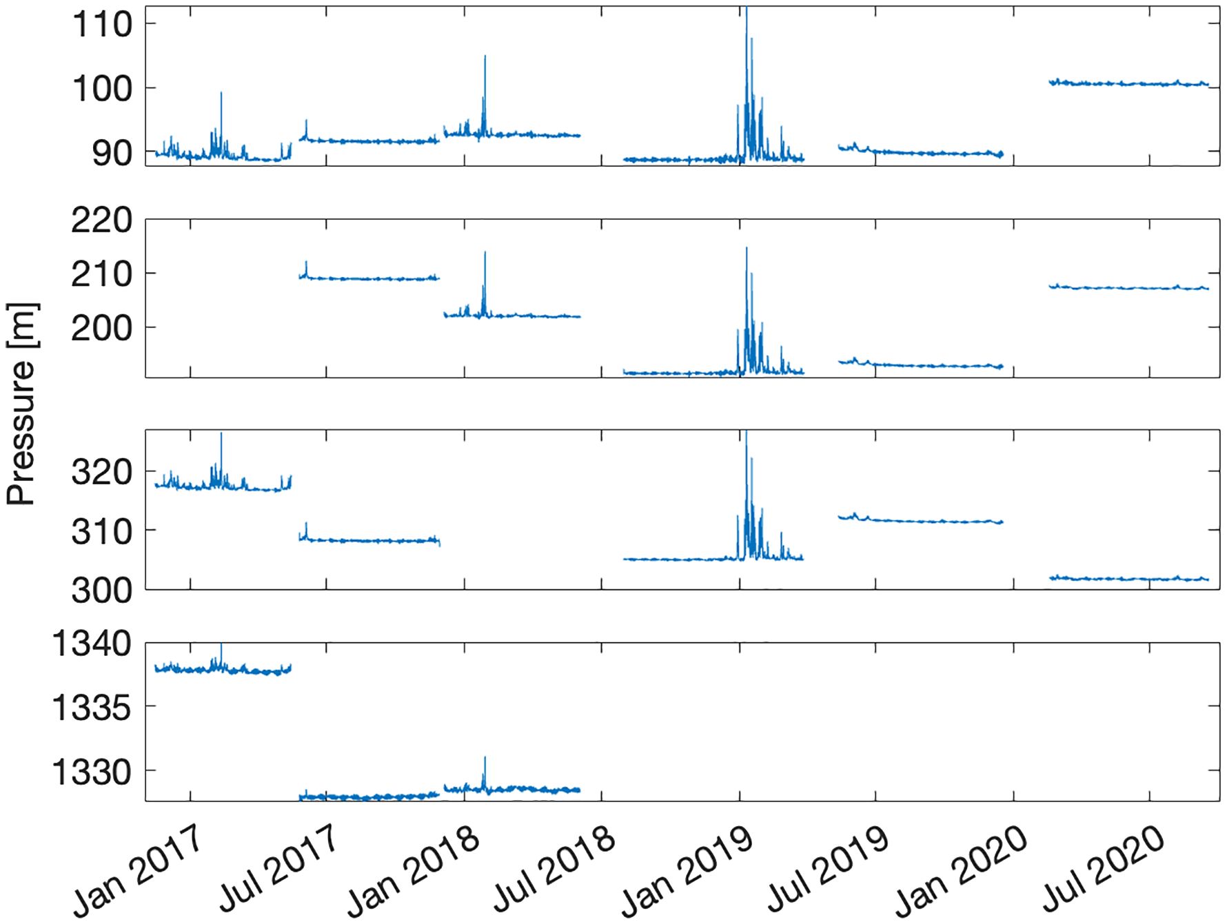
Figure 2 Pressure time series, measured in m, at four depths measured 90 m, 200 m, 300 m, and 1300 m, with each depth shown from top panel to bottom, respectively. Measurements started in November 2016 and ended in June 2020. There were no measurements for all the depths, as described in Supplementary Table 1. Each deployment was measured at a slightly different depth, which is the reason for the differences in pressure between deployment periods.

Figure 3

Figure 3 Temperature and pressure time series, measured in degrees Celsius and m, at three depths measured: 90 m, 200 m, and 300 m, with each depth shown from top panel to bottom, respectively measured between 17 December 2018 and 27 March 2019.

3.1.1 Tidal analysis of pressure variability

Several tidal constituents are evident in the pressure variability. The foremost semidiurnal and diurnal tides—S2, M2, K1, and O1—are shown in Figure 4 as the significant spectral peaks below the fortnightly band, varying slightly between years and depths (Supplementary Table 2). This suggests a barotropic structure with depth-locked amplitude and phase, aligning with models calibrated with experimental results (Tsimplis et al., 1995; Arabelos et al., 2011) and time series data from the western Mediterranean (Albérola et al., 1995). The phases of the tidal constituents are provided in Supplementary Table 3.

Figure 4

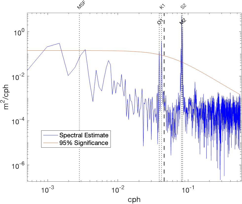
Figure 4 The Power Spectral Density in m² cph^-1 of the pressure time series as a function of cph (log—log) at 300 m depth in the summer of 2017. The dashed vertical lines in the graph indicate tide constituents: Msf, O1, K1, M2, and S2. The red curve indicates the 95% Significance Level with respect to red noise. The diurnal and semidiurnal amplitudes are significant in the spectrum. The MSF fortnightly oscillation peak is seen to be insignificant in the spectral analysis as opposed to the tidal harmonic analysis.

The M2 amplitude is the most dominant and consistent, showing no evident seasonal or depth variability. The average and median amplitudes of the M2 across all depths and seasons are approximately 11.3 cm, which agrees with tide gauges (Tsimplis et al., 1995), models (Tsimplis et al., 1995; Arabelos et al., 2011) and the OSU TPXO barotropic model (Egbert and Erofeeva, 2002) with an amplitude of 10.7 cm. The variance of the M2 across seasons and depths is 0.2 cm², with outlier amplitudes of 9.2 cm and above 12 cm found in some winters, with error estimates of over 2 cm. The S2 amplitude ranges between 5.6—8.3 cm, showing seasonal variability but no depth variability (Figure 5), with fall averaging 8.2 cm and summer averaging 6.1 cm. Previous studies (Tsimplis et al., 1995; Arabelos et al., 2011) reported an S2 range of 7—8 cm, while the OSU TPXO shows 6.2 cm. The O1 ranges between 2—3 cm, with exceptional amplitudes of 10 cm found at all depths of winter 2017, which is larger than the previously observed and modeled results of 1—2 cm, and the OSU TPXO showing 1.9 cm. The K1 tide shows seasonal variation, with larger amplitudes in winter (~10 cm) at 90 m depth and summer amplitudes ranging from 2.5—3.5 cm. At 1300 m, the K1 amplitudes are smaller, ranging from 3.5—4 cm in the winter and 2.5—3 cm in the summer. These results are larger than those predicted or recorded in previous studies of 1—2 cm, with the OSU TPXO showing 1.7 cm.

Figure 5

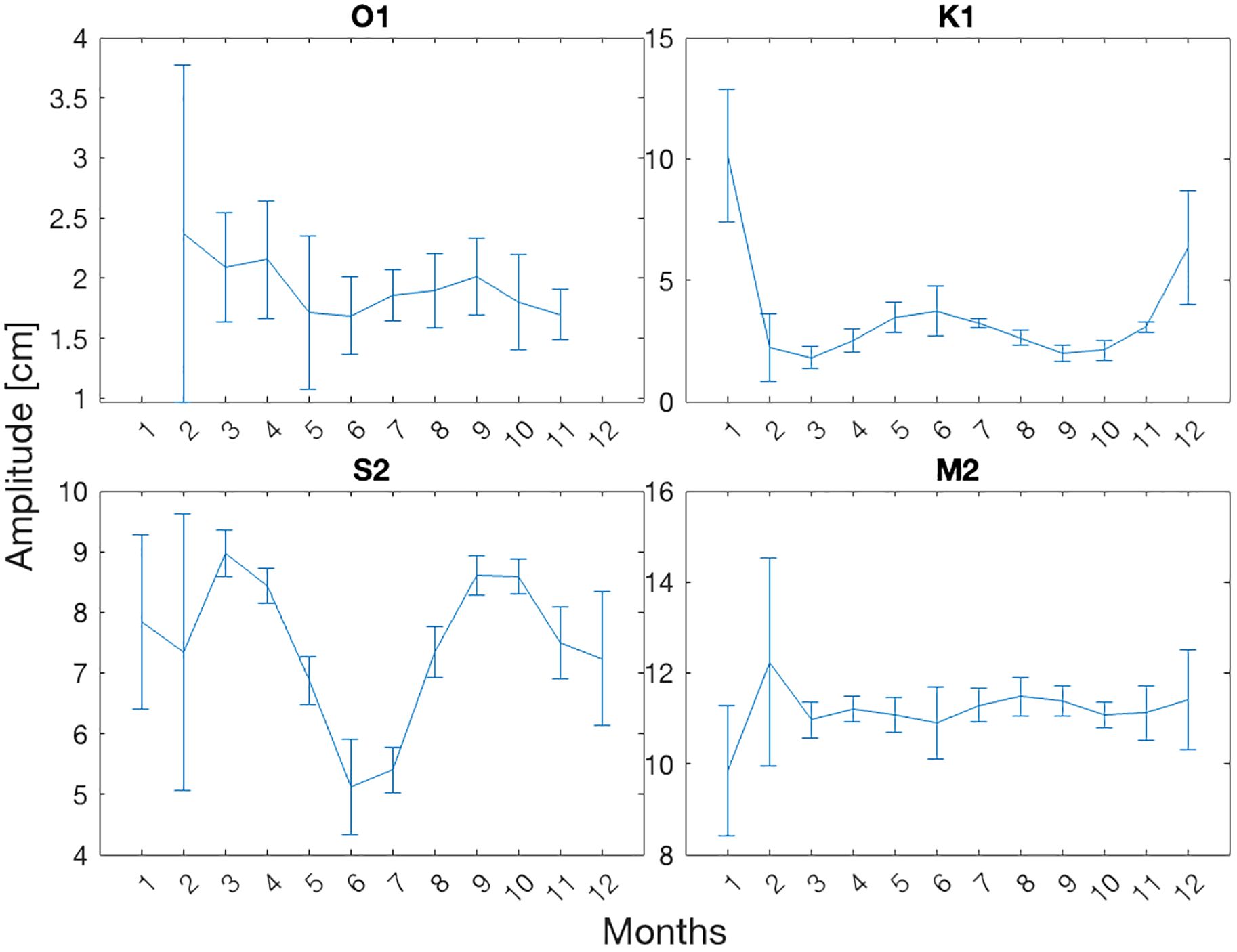
Figure 5 The average monthly amplitudes [cm] of the four major tides analyzed from the 2017—2020 pressure time series at 200 m depth. The vertical lines are average error bars retrieved from the harmonic analysis. The seasonal trends for all the tides are the same at 90 m and 300 m depths.

A fortnightly oscillation is present only in the summers at all depths, as seen in Supplementary Table 2 and the raw pressure data (Figure 6). At the same time, it is not found significant in the spectral analysis shown in Figure 4. This contradiction might be explained by nonlinear interactions between semidiurnal and diurnal tides which have been argued to amplify the oscillations (Kwong et al., 1997). Figure 6 shows a reconstruction of only the M2 and S2 tides, highlighting the spring and neap tides, similar to the fortnightly oscillations observed in the raw data emphasized in the bottom graph.

Figure 6

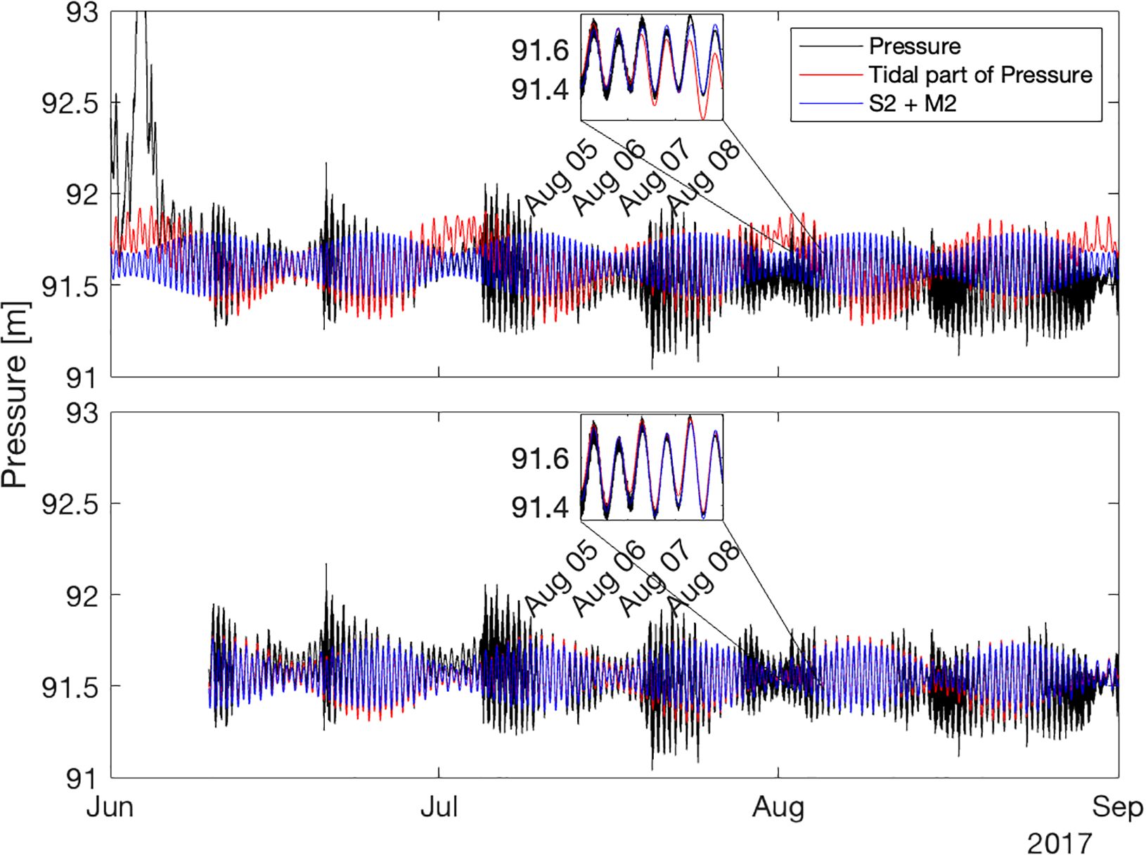
Figure 6 A sample of the pressure time series in m at 90 m from summer 2017 where the top graph includes a sudden pressure jump in the analysis and the bottom graph the pressure jump is excluded from the study. Both graphs include the raw time series (black), the reconstruction of the amplitudes of all the significant tides of the season (red), and the reconstruction of only the S2 and M2 (blue). In the inset, there is a zoom-in on a three-day interval in August. It is clear from both graphs the importance of the significant tides, and specifically the semidiurnal tides, on the pressure. From the zoom-in of both graphs, we can see that the pressure jump distorts the harmonic analysis, where the total reconstruction (red) behaves differently between the two graphs.

Another significant tide identified was the UPS1 tide (Supplementary Table 2). The amplitude range is wide from 0.5—10 cm at 90 m with no clear seasonal pattern apart from winter months, where the largest amplitudes were found.

Tidal constituents represent a significant portion of the variance of the pressure time series for most of the year. The variance variation in 2017 regarding season and depth is demonstrated in Table 2. Notably, the spring variance in 2017 is unusually high, with 2018 and 2020 showing a variance of 1.1*10^-2 m² for all depths apart from 1300 m, for which further data is unavailable. This anomaly can be attributed to the monthly lunar tidal constituent (MM) slightly passing the SNR threshold and contributing to the variance, with an amplitude of around 20 cm. In other years, the MM tide had lower amplitudes and was not significant. The sample length of Spring 2017 is 74.5 days compared to 90 days for the rest of the years, which may contribute to the amplitude leakage into the monthly lunar tidal constituent.

Table 2

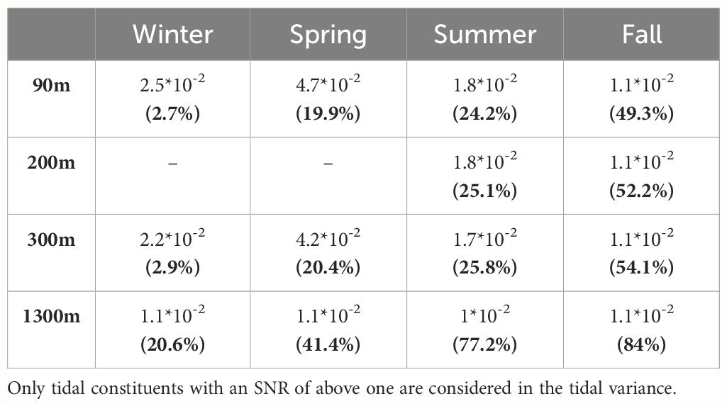
Table 2 Total tidal variance in m² and the percentage of the tidal variance (in bold) from the total variance of the pressure time series found per season of 2017 and at four depths.

Summer and fall percentages in 2017 are uncharacteristically low, with summer percentages around 40% and fall percentages around 70%. While the tidal variance amplitude for summer and fall was similar to those found in other years, an analysis of wind profiles showed slightly larger variance in wind velocity during these seasons in 2017 (not shown). Thus, we can infer that external forces may have caused the unusually high energetic differences in 2017. Nonetheless, the general trends found in Table 2 are relevant and similar for all the years in the study.

With depth, except for fall, there is a slight drop in tidal variance for the top 300 m, stabilizing at a baseline variance of approximately 1.1*10^-2 m² at 1300 m. The proportion of tidal variance in the total variance increases with depth due to diminishing atmospheric influences. At 1300 m, seasonal changes in tidal variance are minimal, though seasonal changes in the tidal variance percentage persist. In the top 300 m, the variance and percentages deviate from the baseline variance in winter and summer across all the years of the dataset, except spring 2017. Winter has the greatest variance, followed by summer, with fall having the highest percentage of tidal variance from the total variance, then summer and spring with roughly similar numbers, and winter with the least tidal variance from the total variance.

3.2 Current variability

Currents were dominated by episodes of strong flows, especially in the winter, as shown in Table 3 and Figures 7, 8. This is due to the winter eddies and the general mesoscale activities characterizing the Levantine basin (Amitai et al., 2010; Solodoch et al., 2023).

Table 3

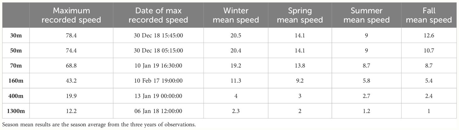
Table 3 Maximum recorded speeds (magnitude of the horizontal currents) at different depths (cm s^-1) were found in all the years of the dataset (cm s^-1) and the dates they were found.

Figure 7

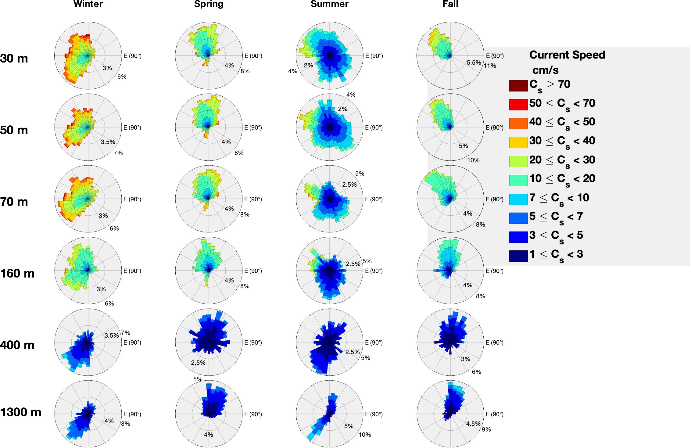
Figure 7 Current rose of the currents at the depths of 30 m, 50 m, 70 m, 160 m, 400 m, and 1300 m during the winter, spring, summer, and fall periods of 2017. The units of the current rose are in cm s^-1. Each record of a given current in a times series is projected in its direction and added to a bin matching the ranges in the legend. The larger the bin size, the more frequently the speed counted in that direction. The approximate frequencies of occurrence can be seen by the percentages shown.

Figure 8

Figure 8 A feather diagram showing the currents (cm s^-1) during winter 2017. Each subplot depicts a different depth, in ascending order of 30 m, 70 m, 160 m, 400 m, and 1300 m. The velocities of the 30 m, 70 m, 160 m, and 1300 m depths were averaged for a two-hour sampling period. Note the different scales for the other depths.

Table 3 shows a decrease in speed with depth and a reduced seasonal dependency at 1300 m due to the diminished impact of atmospheric forces. The flow across the entire water column is mainly meridional (roughly parallel to isobath), as illustrated in the feather diagram in Figure 8. This behavior is explained by the continuous cyclonic boundary current encircling the Levantine basin (Solodoch et al., 2023) coupled with anticyclonic eddies (Amitai et al., 2010).

Near-surface currents predominantly flow northward in the spring. In contrast, summer currents exhibit more sporadic motion (Figure 7). The continental shelf break is parallel to the coast (Figure 1), and in the fall, near-surface currents move perpendicularly away from the shelf. Winter currents move away from the shelf but show no specific direction. At 1300 m depth, current directions alternate between northwest, along the shelf break, during spring and fall, and southeast during the summer and winter. The seasonality of the cyclonic boundary current drives general seasonal current variability. The boundary current strengthens the winter and summer, weakening during the transition seasons. Increased instabilities in the summer occur from the weakening of offshore currents and the absence of submesoscale eddies (Verma et al., manuscript submitted), explaining the sporadic motions in Figure 7.

3.2.1 Tidal harmonic analysis of current variability

The current analysis of the four main tidal constituents (O1, K1, M2, and S2) yields different results than the pressure analysis. Though prominent in the current analysis, the UPS1 tide can be attributed to the near-inertial band and will not be discussed further in the results.

The S2 and M2 tides are significant only sporadically near the surface, with negligible magnitudes of approximately 0.3 cm s^-1 for S2 and 0.3—0.6 cm s^-1 for M2 (Supplementary Table 4). For the M2, this is an order of magnitude weaker than the drifter data found in Poulain et al. (2018). For the S2, the results are consistent with Poulain et al. (2018), showing currents between 0—1 cm s^-1. Drifter data results are generally larger for both the 15 day (0.6—3 cm s^-1) and 30 day (0.7—1.3 cm s^-1) analyses. The OSU TPXO model finds a semimajor axis of the tidal ellipse for the M2 current of 9.7 cm s^-1 and 5.8 cm s^-1 for the S2 tidal current, larger than those in this study. At 1300 m, the S2 and M2 are significant across the seasons, with magnitudes of 0.1—0.2 cm s^-1 for both (Supplementary Table 4). Phases of the tidal constituents are provided in Supplementary Table 5.

An opposite trend is observed for the diurnal tides. At 30 m, the K1 tidal constituent is significant across all seasons, ranging from 0.9—3 cm s^-1 (Supplementary Table 4). Seasonal variability is present, with fall showing the strongest tidal currents and summer—spring the weakest tidal. With depth, K1 is less significant until 1300 m, when the constituent is insignificant across all seasons. This may be due to intense wind stress from the daily breeze, as suggested by Álvarez et al. (2003); Poulain et al. (2018), and others. The O1 tidal currents also decrease with depth, ranging from 0.9—1.9 cm s^-1 at all depths (Supplementary Table 4). In most segments, the analysis did not find significant oscillations of the O1 tide.

The general trends in 2017, shown in Table 4 and the rest of the analyzed data, show stronger tidal currents in the winter and spring and a decrease in the summer, with possible explanations detailed in the discussion section. Similar to the pressure analysis, tidal variance decreases with depth, likely due to atmospheric forces like the diurnal breeze contaminating the tidal analysis. The percentage of tidal variance from total variance increases as near-surface mechanisms weaken. Unlike the pressure analysis, there does not appear to be a baseline variance. The variance of significant tidal constituents plays a minor part in the overall current variance (Table 4), with other mechanisms having a larger impact. Examples of other mechanisms are provided by Feliks et al. (2022), who used the same DeepLev dataset and identified intraseasonal oscillations with periods of 7, 11, 22, and 34–36 days as generally larger (above 4 cm s^-1) than the tides in the eastern Mediterranean shown here.

Table 4

Table 4 Total tidal variance in cm² s^-2 and the percentage of the tidal variance (in bold) from the total variance of the current time series found per season of 2017 and at four depths.

Table 4 shows some inconsistencies with the other years in this research. The top 160 m in winter 2017 are comparatively weaker than other years, which typically have seasonal average magnitudes above 10 cm s^-1 and a higher percentage of variance. A large variance was found in the fall at 70 m, with a comparatively smaller percentage for the top 50 m compared to other years in the same season. At 1300 m in the fall, there is a very low tidal variance, but this cannot be confidently labeled as inconsistent or an outlier due to the lack of available datasets at 1300 m in the fall of other years.

3.2.2 Sensitivity to dataset lengths

Data from four seasons in 2017 from DeepLev was analyzed using tidal harmonic analysis with different dataset lengths of 15, 22, and 30 days at three different depths: 70 m, 160 m, and 1300 m.

At 70 m depth, on average across all seasons, the M2 tide magnitude from a 15 day analysis is approximately 1.3 times larger than the 22 day analysis and 1.6 times larger than the 30 day analysis. For the S2 tide magnitude, a 15 day analysis is approximately 1.1 times larger than a 22 day analysis and 1.4 times larger than a 30 day analysis. The 22 day period is larger than the 30 day, for the M2 magnitude, by only 1.2; for the S2, it is 1.4 times larger.

At 160 m depth, on average across all seasons, the M2 tide magnitude from a 15 day analysis is approximately 1.3 times larger than the 22 day analysis and 1.9 times larger than the 30 day analysis. For the S2 tide magnitude, a 15 day analysis is approximately 1.5 times larger than a 22 day analysis and 1.8 times larger than a 30 day analysis. The 22 day period is larger than the 30 day, for the M2 magnitude, by 1.4; for the S2, it is 1.5 times larger.

At 1300 m depth, on average across all seasons, the M2 tide magnitude from a 15 day analysis is approximately 1.2 times larger than the 22 day analysis and 1.1 times larger than the 30 day analysis. For the S2 tide magnitude, a 15 day analysis is 0.9 times larger than the 22 day analysis (this may be due to a lack of significant tides across the seasons, as shown in Supplementary Table 6) and 1.3 times larger than the 30 day analysis. The 22 day period is the same as the 30 day for the M2 magnitude, while for the S2, it is 1.4 times larger.

These results align with the leakage effects of two close frequencies analyzed at exactly their Rayleigh criterion and not their “well resolved” criterion. In summary, the 15 day analysis for the M2 and S2 results in larger magnitude than the 22 day analysis, which in turn is larger than the 30 day analysis. Supplementary Table 6 contains the detailed results from the tidal harmonic analysis of the mooring data.

3.3 Tidal harmonic analysis based on drifter data vs. moored instruments

We tested the sensitivity of the semidiurnal tidal constituent results from a tidal analysis on drifters using different dataset lengths. The results were compared with current data from DeepLev. The Rayleigh criterion for the S2 and M2 constituents is approximately 15 days, yet the stricter “well-defined” criterion is approximately 22 days. We used 15, 22, and 30 day datasets for our comparative analysis. We used drifter datasets with trajectories within 1° of DeepLev to limit the spatial variations in tidal regimes.

3.3.1 Tidal harmonic analysis of drifter data from 15 day segments

Supplementary Table 7 provides detailed results of the drifter data following a tidal harmonic analysis. For many segments fitting the predefined criteria, the dominant tide was the S2 tide, as shown in Table 5. Interestingly, the S2 results show a decrease in magnitude from the beginning of the summer season, consistent with the results shown in section 3.2.

Table 5

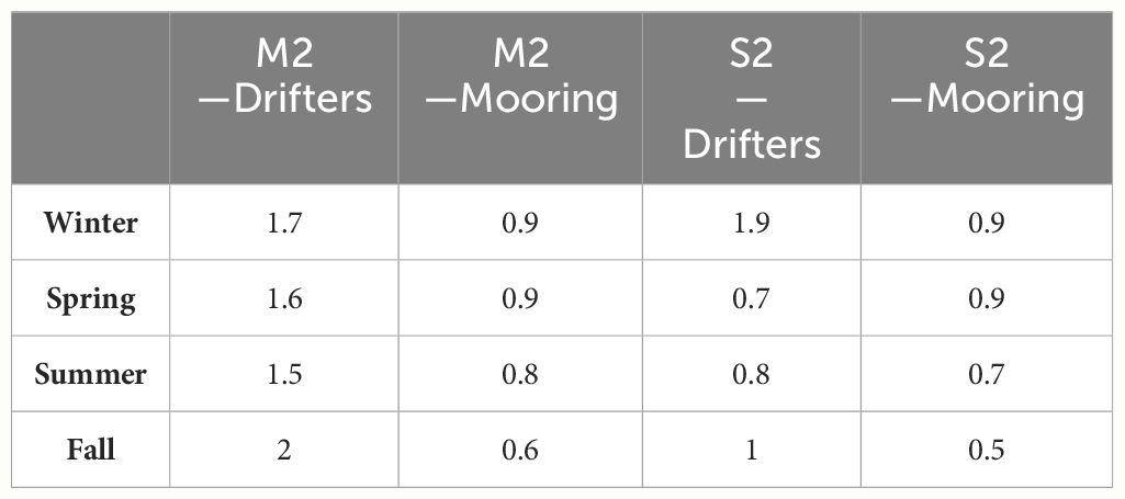
Table 5 Seasonal average magnitudes [cm s^-1] of the M2 and S2 tidal currents from drifters and DeepLev in 15 day segments.

To compare the drifter analysis, we performed a tidal harmonic analysis on data from DeepLev for the same dates at 50 m depth. This analysis did not show a dominant S2 or M2 tidal constituent and generally produced smaller magnitudes than the drifter analysis. This discrepancy might be due to the depth of the moored device, indicating atmospheric influences on the semidiurnal tides. The moored dataset shows that while the semidiurnal tides are nearly the same, the magnitudes reported at DeepLev are much smaller for the S2 tide and only slightly smaller for the M2 tide. The magnitudes from DeepLev are also larger than those found in section 3.2.1, consistent with signal analysis theory. Both DeepLev and drifter results align with Poulain et al. (2018), which observed both the S2 and M2 with magnitudes under 2 cm s^-1.

A few notes are essential. First, the summer results include segments from the summers of 2017 and 2018, unlike other seasons, for which there were only datasets from 2017. Lastly, the S2 and M2 magnitude behavior—S2 being greater than M2—was observed in different drifter types and years, strengthening the argument that the S2 tidal constituent is larger on the surface than the M2 constituent.

3.3.2 Tidal harmonic analysis of drifter data from 22 day segments

The results from the drifters’ 22 day segments, shown in Table 6, were generally smaller in magnitude than the 15 day segments, consistent with theory and section 3.2.2. The dominant S2 observed in the 15 day drifters subsided and is almost the same as the M2, except for the summer and fall results, with fall containing only one segment. The magnitudes from DeepLev were roughly the same for both the 15 and 22 day segments. Notably, raising the time limit to 22 days resulted in fewer segments and fewer significant tidal results. Detailed results of the relevant drifter segments following a tidal harmonic analysis can be found in Supplementary Table 8.

Table 6

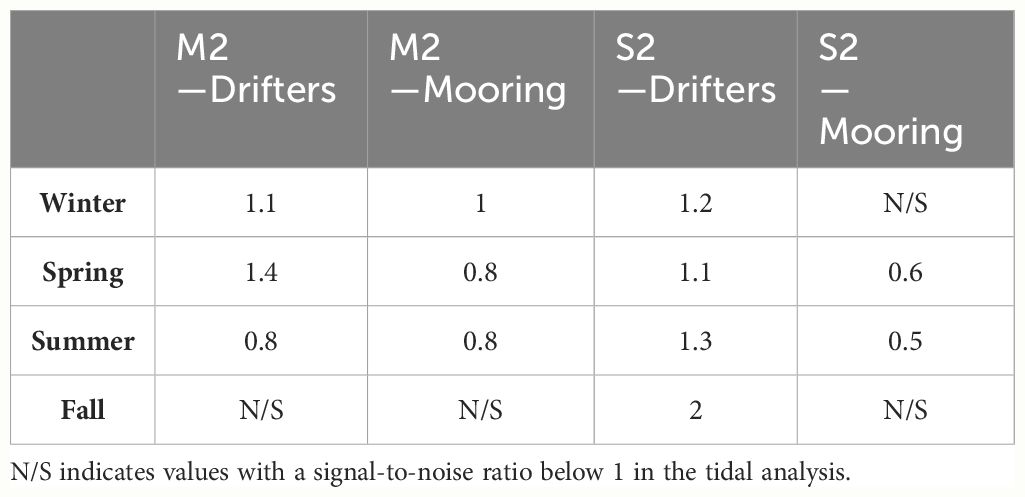
Table 6 Seasonal average magnitudes [cm s^-1] of the M2 and S2 tidal currents from drifters and DeepLev in 22 day segments.

3.3.3 Tidal harmonic analysis of drifter data from 30 day segments

Only seven 30 day drifter segments were found near DeepLev. A summary of the results are shown in Table 7. Detailed results of the drifter data following a tidal harmonic analysis can be found in Supplementary Table 9. Unfortunately, a gap in the mooring data coincided with the proximity of the drifters, resulting in only a few comparable datasets. An example of a drifter’s 30 day trajectory can be found in Supplementary Figure 1. The drifter’s trajectory is similar to those observed in drifters with near-inertial oscillations or motions.

Table 7

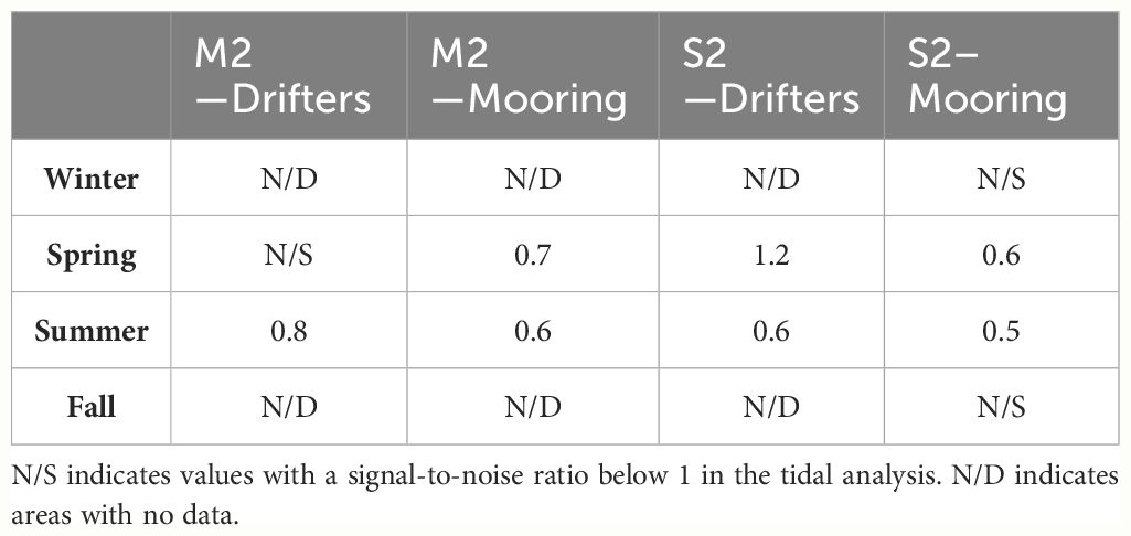
Table 7 Seasonal average magnitudes [cm s^-1] of the M2 and S2 tidal currents from drifters and DeepLev in 30 day segments.

In summary, the tidal harmonic analysis on different drifter dataset lengths shows a weakening in the magnitude of the M2 and S2 tide as the dataset length increases. This trend was less pronounced in the equivalent mooring dataset but remained evident.

4 Discussion

The data collected from both the mooring station and surface drifters in its vicinity provide a comprehensive view of the tidal structure in the eastern Levantine Basin. This includes semidiurnal (M2 and S2), diurnal (K1 and O1), and longer-period (Msf) tides. The pressure variance explained by the tides is substantial in all seasons except winter, with fall showing the highest explained variance (average of 67%), which increases with depth. In contrast, the current variance explained by the tides is less considerable, shows slight variation with depth, and peaks in spring (average of 19%). A much larger portion of the variance is attributed to intraseasonal variability (Feliks et al., 2022).

The M2 tide is the most dominant frequency, with amplitudes similar to those observed in tide gauges and models (Tsimplis et al., 1995; Arabelos et al., 2011). There is no evident seasonal variability in the M2 amplitude. For the S2 tide, an amplitude change of 2 cm is observed between summer and fall averages. Despite this variability, previous studies and the OSU TPXO model show that this range generally agrees with previous results. Seasonal variations of tides can result from several factors. Müller et al. (2014) suggested that stronger stratification leads to less energy loss from the barotropic tide to turbulence and mixing. Our research finds that the amplitudes in summer are weaker than in spring and fall, as seen in Figure 5, with seasonality influences also observed in the 300 m dataset. While stratification is generally stronger in summer in the Levantine basin (Hecht et al., 1988), it might not be the main driver of seasonality, as the permanent thermocline starts at 140 m. Verma et al. (Submitted manuscript) have shown that instabilities in the water column occur in the summer in the eastern Levantine basing. Ozer et al. (2022) report a salinity minimum in August near the Israeli coast due to the intensification of the along-shore currents in June-July. Rosentraub and Brenner (2007) identified an along-slope baroclinic jet in the summer. These instabilities may cause energy loss due to increased turbulence and mixing. Ray (2022) proposed that compound tides with frequencies near the M2 tide, as well as astronomical modulations of the Sun’s third body perturbations of the lunar orbit, play a role in the observed seasonality of the M2 tide. Alongside atmospheric processes, these mechanisms may play a role in the S2 seasonal variation.

Sharp variability due to seasonal change and depths was found in the K1 signal, with amplitudes reaching up to 10 cm in winter near the surface, significantly higher than previously reported, and down to 2-3 cm in summer, slightly larger than the models and observations. Although not within the scope of this paper, preliminary seasonal spectral analysis of coastal wind speed from a meteorological site on the Israeli coast shows strong semidiurnal and diurnal frequencies during winter compared to the rest of the year. Another possible explanation for these results is mooring motions unrelated to the tides.

The large fluctuations found in the pressure data during winter, specifically in Jan 2019, might be due to the tilting of the mooring device from strong horizontal motions (Katz et al., 2020). The tilt needed to move the devices vertically by 22 m, the approximate maximum vertical variation seen in Figure 3, is about 10.5 degrees, giving a horizontal deviation of 236.9 m. These currents could result from a mesoscale eddy passing in the area of DeepLev, as the Levantine basin is dominated by mesoscale activities, with anticyclonic mesoscale eddies reported in the DeepLev area (Amitai et al., 2010; Solodoch et al., 2023). Feliks and Itzikowitz (1987) showed that eddies in the eastern Mediterranean could create localized temperature increases at depths down to 300 m. Figure 3 shows localized temperature increases similar to those described by Feliks and Itzikowitz (1987). Additionally, synoptic maps (not shown) of pressure from NCEP reanalysis in January do not display any storm in the area.

The O1 and K1 tides exhibit anomalously high amplitudes in winter, significantly larger than previously observed. This heightened amplitude could be due to the leakage of the inertial period into the diurnal frequencies caused by winter eddies near DeepLev, such as the one showcased in section 3.1. Another explanation for the seasonal variation in O1 and K1 tides is a resonant mechanism with the diurnal breeze, which can generate near-inertial waves that leak into the diurnal frequencies (Mihanović et al., 2016). However, this explanation seems unlikely because the diurnal wind frequencies during winter were less energetic than those in summer and fall of 2017, as shown in the wind PSD in Supplementary Figure 2.

For all seasons, the weak semidiurnal tidal currents observed from the mooring device are consistent with the literature (Pugh, 1987; Poulain et al., 2018) with magnitudes below 1 cm s^-1. Our results indicate that semidiurnal tides are only sporadically significant near the surface, whereas at 1300 m depth, they were significant across all seasons. This disparity is likely due to stronger near-surface currents dominated by non-tidal influences. Diurnal tides, particularly the K1 tide, exhibit amplitudes above 1 cm s^-1 near the surface across all the seasons, with fall currents averaging 2.2 cm s^-1. These elevated diurnal tides might be attributed to the diurnal breeze present in all seasons.

Additional noteworthy tidal constituents were identified in the analysis. The most dominant tidal current observed was the UPS1 tide, with magnitudes reaching up to 5 cm s^-1. This constituent is significant in all seasons and depths. In contrast, the UPS1 oscillation is less dominant in the pressure analysis than in the current data, as detailed in section 3.2.1. The UPS1 tide has been observed in sea level variability studies using tide gauges along the Port of Alexandria (El-Geziry and Radwan, 2012; Khedr et al., 2018; El-Geziry, 2021), with amplitudes below 1.5 cm. However, the UPS1 tide observed here could be attributed to near-inertial internal waves, given the clockwise motion of the currents when the UPS1 tide is present (not shown). Near-inertial motions generate internal waves that oscillate both horizontally and vertically, albeit with smaller vertical amplitudes than internal tides (Alford et al., 2016). The amplitude of this tidal constituent decreases with depth across all seasons, consistent with near-inertial oscillations. Drifter data from the eastern Mediterranean (Poulain et al., 2023) indicate shifts in the effective near-inertial frequency due to mesoscale eddies, which may contribute to our findings. When analyzing larger datasets (e.g., 120 day and 180 day periods, not shown), we found that the dominant frequency shifts away from the UPS1 tide and closer to 21.99 h, the inertial frequency at DeepLev. This is also supported by the rotary spectra of the current time series, which show a predominantly clockwise motion (not shown).

As mentioned in the introduction, previous studies in the eastern Mediterranean have documented the fortnightly tidal constituents (Msf, Mf). In our results, the fortnightly tide was significant in only a few analyzed datasets. Further detailed studies are necessary to understand the mechanisms behind the existence and impacts of fortnightly tides in the Levantine Basin.

The DeepLev mooring station allowed us to assess the temporal resolution criteria needed for surface drifters to provide an accurate representation of the local tidal regime. The findings in sections 3.2.2 and 3.3.1 illustrate the leakage of M2 and S2 tides in the tidal analysis due to “just resolved” peaks in this local scenario. Although we observed large amplitude changes when analyzing different dataset lengths, the number of relevant drifters near DeepLev decreased with each dataset length, posing a challenge when adopting stricter temporal constraints. All the results obtained from surface drifters, regardless of dataset length, showed were larger amplitudes (>1 cm s^-1) compared to those from moored datasets (<1 cm s^-1).

Data availability statement

The datasets presented in this study can be found in online repositories. The names of the repository/repositories and accession number(s) can be found in the article/Supplementary Material.

Author contributions

NM: Conceptualization, Data curation, Formal analysis, Funding acquisition, Investigation, Methodology, Project administration, Resources, Software, Supervision, Validation, Visualization, Writing – original draft, Writing – review & editing. YF: Conceptualization, Methodology, Validation, Writing – original draft, Writing – review & editing. HG: Conceptualization, Data curation, Formal analysis, Funding acquisition, Investigation, Methodology, Project administration, Resources, Software, Supervision, Validation, Visualization, Writing – original draft, Writing – review & editing. PP: Conceptualization, Data curation, Investigation, Methodology, Software, Supervision, Validation, Writing – original draft, Writing – review & editing. EM: Data curation, Formal analysis, Investigation, Resources, Validation, Visualization, Writing – original draft, Writing – review & editing. MM: Data curation, Resources, Software, Validation, Writing – original draft, Writing – review & editing.

Funding

The author(s) declare financial support was received for the research, authorship, and/or publication of this article. This study was supported by the Israeli Ministry of Science and the Italian Ministry of Foreign Affairs.

Acknowledgments

DeepLev station operation was partially supported by the North American Friends of IOLR, by the Medi- terranean Sea Research Center of Israel (MERCI), and by an ISF grant to Yishai Weinstein and Ilana Berman-Frank No.25/14. We thank Yishai Weinstein and Ronen Alkalay from Bar-Ilan University, Timor Katz and Barak Herut from IOLR, and Ilana Berman-Frank from Haifa University for leading the DeepLev project, and the staff of IOLR for invaluable help with marine and technical operations. We thank Shayna Moliver and Alex Moliver for their suggestions and improvements to the manuscript.

Conflict of interest

The authors declare that the research was conducted in the absence of any commercial or financial relationships that could be construed as a potential conflict of interest.

Publisher’s note

All claims expressed in this article are solely those of the authors and do not necessarily represent those of their affiliated organizations, or those of the publisher, the editors and the reviewers. Any product that may be evaluated in this article, or claim that may be made by its manufacturer, is not guaranteed or endorsed by the publisher.

Supplementary material

The Supplementary Material for this article can be found online at: https://www.frontiersin.org/articles/10.3389/fmars.2024.1388137/full#supplementary-material

References

Albérola C., Rousseau S., Millot C., Astraldi M., Font J., García-Lafuente J., et al. (1995). Tidal currents in the western Mediterranean Sea. Oceanologica Acta 18, 273–284.

Google Scholar

Alford M. H., MacKinnon J. A., Simmons H. L., Nash J. D. (2016). Near-inertial internal gravity waves in the ocean. Annu. Rev. Mar. Sci. 8, 95–123. doi: 10.1146/annurev-marine-010814-015746

CrossRef Full Text | Google Scholar

Álvarez O., Tejedor B., Tejedor L., Kagan B. A. (2003). A note on sea-breeze-induced seasonal variability in the K1 tidal constants in Cádiz Bay, Spain. Estuarine Coast. Shelf Sci. 58, 805–812. doi: 10.1016/S0272-7714(03)00186-0

CrossRef Full Text | Google Scholar

Amitai Y., Lehahn Y., Lazar A., Heifetz E. (2010). Surface circulation of the eastern Mediterranean Levantine basin: Insights from analyzing 14 years of satellite altimetry data. J. Geophys. Res.: Oceans 115(C10), C10058. doi: 10.1029/2010JC006147

CrossRef Full Text | Google Scholar

Arabelos D. N., Papazachariou D. Z., Contadakis M. E., Spatalas S. D. (2011). A new tide model for the Mediterranean Sea based on altimetry and tide gauge assimilation. Ocean Sci. 7, 429–444. doi: 10.5194/os-7-429-2011

CrossRef Full Text | Google Scholar

Bendat J. S., Piersol A. G. (2011). Random data: analysis and measurement procedures (Hoboken, NJ: John Wiley & Sons).

Google Scholar

Carrère L., Le Provost C., Lyard F. (2004). On the statistical stability of the M2 barotropic and baroclinic tidal characteristics from along-track TOPEX/Poseidon satellite altimetry analysis. J. Geophys. Res.: Oceans 109 (C3), C03033. doi: 10.1029/2003JC001873

CrossRef Full Text | Google Scholar

Chavanne C., Janeković I., Flament P., Poulain P. M., Kuzmić M., Gurgel K. W. (2007). Tidal currents in the northwestern Adriatic: High-frequency radio observations and numerical model predictions. J. Geophys. Res.: Oceans 112(C3), C03S21. doi: 10.1029/2006JC003523

CrossRef Full Text | Google Scholar

Cosoli S., Drago A., Ciraolo G., Capodici F. (2015). Tidal currents in the Malta–Sicily Channel from high-frequency radar observations. Continental Shelf Res. 109, 10–23. doi: 10.1016/j.csr.2015.08.030

CrossRef Full Text | Google Scholar

Crawford W. R., Cherniawsky J. Y., Cummins P. F., Foreman M. G. G. (1998). Variability of tidal currents in a wide strait: A comparison between drifter observations and numerical simulations. J. Geophys. Res.: Oceans 103 (C6), 12743–12759.

Google Scholar

Deparis V., Legros H., Souchay J. (2013). “Investigations of tides from the antiquity to laplace,” Tides in astronomy and astrophysics (Berlin, Heidelberg: Springer Berlin Heidelberg), 31–82. doi: 10.1007/978-3-642-32961-6_2

CrossRef Full Text | Google Scholar

Egbert G. D., Erofeeva S. Y. (2002). Efficient inverse modeling of barotropic ocean tides. J. Atmospheric Oceanic Technol. 19, 183–204. doi: 10.1175/1520-0426(2002)019<0183:EIMOBO>2.0.CO;2

CrossRef Full Text | Google Scholar

El-Geziry T., Radwan A. (2012). Sea level analysis off Alexandria, Egypt. Egypt. J. Aquat. Res. 38, 1–5. doi: 10.1016/j.ejar.2012.08.004

CrossRef Full Text | Google Scholar

El-Geziry T. M. (2021). Sea-level, tides and residuals in Alexandria Eastern Harbour, Egypt. Egypt. J. Aquat. Res. 47, 29–35. doi: 10.1016/j.ejar.2020.10.003

CrossRef Full Text | Google Scholar

Feliks Y., Itzikowitz S. (1987). Movement and geographical distribution of anticyclonic eddies in the Eastern Levantine Basin. Deep Sea Res. Part A. Oceanographic Res. Papers 34, 1499–1508. doi: 10.1016/0198-0149(87)90105-1

CrossRef Full Text | Google Scholar

Feliks Y., Gildor H., Mantel N. (2022). Intraseasonal oscillatory modes in the Eastern Mediterranean Sea. J. Phys. Oceanogr. 52 (7), 1471–1482. doi: 10.1175/JPO-D-21-0185.1

CrossRef Full Text | Google Scholar

Ferrarin C., Bellafiore D., Sannino G., Bajo M., Umgiesser G. (2018). Tidal dynamics in the inter-connected Mediterranean, Marmara, Black and Azov seas. Prog. Oceanogr. 161, 102–115. doi: 10.1016/j.pocean.2018.02.006

CrossRef Full Text | Google Scholar

Foreman M. G. G. (1977). Manual for tidal heights analysis and prediction (Patricia Bay: Institute of Ocean Sciences).

Google Scholar

Garcia-Gorriz E., Candela J., Font J. (2003). Near-inertial and tidal currents detected with a vessel-mounted acoustic Doppler current profiler in the western Mediterranean Sea. J. Geophys. Res.: Oceans 108(C5), 3164. doi: 10.1029/2001JC001239

CrossRef Full Text | Google Scholar

Gasparini G. P., Smeed D. A., Alderson S., Sparnocchia S., Vetrano A., Mazzola S. (2004). Tidal and subtidal currents in the Strait of Sicily. J. Geophys. Res.: Oceans 109(C2), C02011. doi: 10.1029/2003JC002011

CrossRef Full Text | Google Scholar

Hansen D. V., Poulain P. M. (1996). Processing of WOCE/TOGA drifter data. J. Atmospheric Oceanic Technol. 13, 900–909. doi: 10.1175/1520-0426(1996)013<0900:QCAIOW>2.0.CO;2

CrossRef Full Text | Google Scholar

Hecht A., Pinardi N., Robinson A. R. (1988). Currents, water masses, eddies and jets in the Mediterranean Levantine Basin. J. Phys. Oceanogr. 18, 1320–1353. doi: 10.1175/1520-0485(1988)018<1320:CWMEAJ>2.0.CO;2

CrossRef Full Text | Google Scholar

Katz T., Weinstein Y., Alkalay R., Biton E., Toledo Y., Lazar A., et al. (2020). The first deep-sea mooring station in the eastern Levantine basin (DeepLev), outline and insights into regional sedimentological processes. Deep Sea Res. Part II: Topical Stud. Oceanogr. 171, 104663. doi: 10.1016/j.dsr2.2019.104663

CrossRef Full Text | Google Scholar

Khedr A. M., Abdelrahman S. M., El-Din K. A. A. (2018). Currents and sea level variability of Alexandria coast in association with wind forcing. J. King Abdulaziz Univ. 28, 27–42. doi: 10.4197/Mar.28-2.3

CrossRef Full Text | Google Scholar

Kodaira T., Thompson K. R., Bernier N. B. (2016). Prediction of M2 tidal surface currents by a global baroclinic ocean model and evaluation using observed drifter trajectories. J. Geophys. Res.: Oceans 121 (8), 6159–6183.

Google Scholar

Kunze E. (1985). Near-inertial wave propagation in geostrophic shear. J. Phys. Oceanogr. 15, 544–565. doi: 10.1175/1520-0485(1985)015<0544:NIWPIG>2.0.CO;2

CrossRef Full Text | Google Scholar

Kwong S. C., Davies A. M., Flather R. A. (1997). A three-dimensional model of the principal tides on the European shelf. Prog. Oceanogr. 39, 205–262. doi: 10.1016/S0079-6611(97)00014-1

CrossRef Full Text | Google Scholar

Lafuente J. M. G., Lucaya N. C. (1994). Tidal dynamics and associated features of the northwestern shelf of the Alboran Sea. Continental Shelf Res. 14, 1–21. doi: 10.1016/0278-4343(94)90002-7

CrossRef Full Text | Google Scholar

Lie H. J., Lee S., Cho C. H. (2002). Computation methods of major tidal currents from satellite-tracked drifter positions, with application to the Yellow and East China Seas. J. Geophys. Res.: Oceans 107, 3–1. doi: 10.1029/2001JC000898

CrossRef Full Text | Google Scholar

Lilly J. M. (2021). jLab: A data analysis package for Matlab, v.1.7.1. Available online at: http://www.jmlilly.net/software.

Google Scholar

Medvedev I. P., Vilibić I., Rabinovich A. B. (2020). Tidal resonance in the Adriatic Sea: Observational evidence. J. Geophys. Res.: Oceans 125, e2020JC016168. doi: 10.1029/2020JC016168

CrossRef Full Text | Google Scholar

Menna M., Poulain P. M., Bussani A., Gerin R. (2018). Detecting the drogue presence of SVP drifters from wind slippage in the Mediterranean Sea. Measurement 125, 447–453. doi: 10.1016/j.measurement.2018.05.022

CrossRef Full Text | Google Scholar

Mihanović H., Pattiaratchi C., Verspecht F. (2016). Diurnal sea breezes force near-inertial waves along Rottnest continental shelf, southwestern Australia. J. Phys. Oceanogr. 46, 3487–3508. doi: 10.1175/JPO-D-16-0022.1

CrossRef Full Text | Google Scholar

Millot C., Garcia-Lafuente J. (2011). About the seasonal and fortnightly variabilities of the Mediterranean outflow. Ocean Sci. 7, 421–428. doi: 10.1016/j.measurement.2018.05.022

CrossRef Full Text | Google Scholar

Müller M., Cherniawsky J. Y., Foreman M. G., von Storch J. S. (2014). Seasonal variation of the M 2 tide. Ocean Dynamics 64, 159–177. doi: 10.1007/s10236-013-0679-0

CrossRef Full Text | Google Scholar

Ohshima K. I., Wakatsuchi M., Fukamachi Y., Mizuta G. (2002). Near-surface circulation and tidal currents of the Okhotsk Sea observed with satellite-tracked drifters. J. Geophys. Res.: Oceans (Chicago) 107 (C11), 16–11.

Google Scholar

Ozer T., Gertman I., Gildor H., Herut B. (2022). Thermohaline temporal variability of the SE Mediterranean coastal waters (Israel)–long-term trends, seasonality, and connectivity. Front. Mar. Sci. 8, 799457. doi: 10.3389/fmars.2021.799457

CrossRef Full Text | Google Scholar

Palma M., Iacono R., Sannino G., Bargagli A., Carillo A., Fekete B. M., et al. (2020). Short-term, linear, and non-linear local effects of the tides on the surface dynamics in a new, high-resolution model of the Mediterranean Sea circulation. Ocean Dyn. 70, 935–963. doi: 10.1007/s10236-020-01364-6

CrossRef Full Text | Google Scholar

Pawlowicz R. (2020). “M_Map: A mapping package for MATLAB”, version 1.4m. Available online at: www.eoas.ubc.ca/~rich/map.html.

Google Scholar

Pawlowicz R., Beardsley B., Lentz S. (2002). Classical tidal harmonic analysis including error estimates in MATLAB using T_TIDE. Comput. Geosci. 28, 929–937. doi: 10.1016/S0098-3004(02)00013-4

CrossRef Full Text | Google Scholar

Percival D. B., Walden A. T. (1993). Spectral analysis for physical applications (Cambridge University Press).

Google Scholar

Perkins H. (1976). Observed effect of an eddy on inertial oscillations. Deep Sea Res. Oceanographic Abstracts 23, 1037–1042. doi: 10.1016/0011-7471(76)90879-2

CrossRef Full Text | Google Scholar

Poulain P. M., Bussani A., Gerin R., Jungwirth R., Mauri E., Menna M., et al. (2013). Mediterranean surface currents measured with drifters: From basin to subinertial scales. Oceanography 26, 38–47. doi: 10.5670/oceanog.2013.03

CrossRef Full Text | Google Scholar

Poulain P. M., Centurioni L. (2015). Direct measurements of W orld O cean tidal currents with surface drifters. J. Geophys. Res.: Oceans 120, 6986–7003. doi: 10.1002/2015JC010818

CrossRef Full Text | Google Scholar

Poulain P. M., Menna M., Gerin R. (2018). Mapping Mediterranean tidal currents with surface drifters. Deep Sea Res. Part I: Oceanographic Res. Papers 138, 22–33. doi: 10.1016/j.dsr.2018.07.011

CrossRef Full Text | Google Scholar

Poulain P. M., Menna M., Mauri E. (2012). Surface geostrophic circulation of the Mediterranean Sea derived from drifter and satellite altimeter data. J. Phys. Oceanogr. 42, 973–990. doi: 10.1175/JPO-D-11-0159.1

CrossRef Full Text | Google Scholar

Poulain P.-M., Menna M., Mauri E., Pirro A., Hayes D. R., Gildor H. (2023). Drifter observations of surface currents in the Cyprus Gyre. Front. Mar. Sci. 10. doi: 10.3389/fmars.2023.1266040

CrossRef Full Text | Google Scholar

Poulain P. M., Zambianchi E. (2007). Surface circulation in the central Mediterranean Sea as deduced from Lagrangian drifters in the 1990s. Continental Shelf Res. 27, 981–1001. doi: 10.1016/j.csr.2007.01.005

CrossRef Full Text | Google Scholar

Pugh D. T. (1987). Tides, surges and mean sea level (New York, New York: John Wiley and Sons).

Google Scholar

Ray R. D. (2022). On seasonal variability of the M 2 tide. Ocean Sci. 18, 1073–1079. doi: 10.5194/os-18-1073-2022

CrossRef Full Text | Google Scholar

Rosentraub Z., Brenner S. (2007). Circulation over the southeastern continental shelf and slope of the Mediterranean Sea: direct current measurements, winds, and numerical model simulations. J. Geophys. Res.: Oceans 112, C11001. doi: 10.1029/2006JC003775

CrossRef Full Text | Google Scholar

Sammartino S., García Lafuente J., Naranjo C., Sánchez Garrido J. C., Sánchez Leal R., Sánchez Román A. (2015). Ten years of marine current measurements in E spartel Sill, Strait of Gibraltar. J. Geophys. Res.: Oceans 120, 6309–6328. doi: 10.1002/2014JC010674

CrossRef Full Text | Google Scholar

Sannino G., Carillo A., Pisacane G., Naranjo C. (2015). On the relevance of tidal forcing in modelling the Mediterranean thermohaline circulation. Prog. Oceanogr. 134, 304–329. doi: 10.1016/j.pocean.2015.03.002

CrossRef Full Text | Google Scholar

Slepian D. (1978). Prolate spheroidal wave functions, Fourier analysis, and uncertainty—V: The discrete case. Bell System Tech. J. 5, 1371–1430. doi: 10.1002/bltj.1978.57.issue-5

CrossRef Full Text | Google Scholar

Solodoch A., Barkan R., Verma V., Gildor H., Toledo Y., Khain P., et al. (2023). Basin-scale to submesoscale variability of the east mediterranean sea upper circulation. J. Phys. Oceanogr. 53, 2137–2158. doi: 10.1175/JPO-D-22-0243.1

CrossRef Full Text | Google Scholar

Soto-Navarro J., Lorente P., Alvarez Fanjul E., Carlos Sánchez-Garrido J., García-Lafuente J. (2016). Surface circulation at the Strait of Gibraltar: A combined HF radar and high resolution model study. J. Geophys. Res.: Oceans 121, 2016–2034. doi: 10.1002/2015JC011354

CrossRef Full Text | Google Scholar

Thomson D. J. (1982). Spectrum estimation and harmonic analysis. Proc. IEEE 70, 1055–1096. doi: 10.1109/PROC.1982.12433

CrossRef Full Text | Google Scholar

Thomson R. E., Emery W. J. (2014). Data analysis methods in physical oceanography, 3rd edn (Newnes: Elsevier).

Google Scholar

Tsimplis M. N., Bryden H. L. (2000). Estimation of the transports through the Strait of Gibraltar. Deep Sea Res. Part I: Oceanographic Res. Papers 47, 2219–2242. doi: 10.1016/S0967-0637(00)00024-8

CrossRef Full Text | Google Scholar

Tsimplis M. N., Proctor R., Flather R. A. (1995). A two-dimensional tidal model for the Mediterranean Sea. J. Geophys. Res.: Oceans 100, 16223–16239. doi: 10.1029/95JC01671

CrossRef Full Text | Google Scholar

Ursella L., Kovačević V., Gačić M. (2014). Tidal variability of the motion in the Strait of Otranto. Ocean Sci. 10, 49–67. doi: 10.5194/os-10-49-2014

CrossRef Full Text | Google Scholar

Vilibić I., Šepić J., Dadić V., Mihanović H. (2010). Fortnightly oscillations observed in the Adriatic Sea. Ocean Dyn. 60, 57–63. doi: 10.1007/s10236-009-0241-2

CrossRef Full Text | Google Scholar

Wang D., Pan H., Jin G., Lv X. (2020). Seasonal variation of the principal tidal constituents in the Bohai Sea. Ocean Sci. 16, 1–14. doi: 10.5194/os-16-1-2020

CrossRef Full Text | Google Scholar

Zaron E. D., Elipot S. (2020). An assessment of global ocean barotropic tide models using geodetic mission altimetry and surface drifters. J. Phys. Oceanogr. 51 (1), 63–82.

Google Scholar

Zaron E. D., Ray R. D. (2017). Using an altimeter-derived internal tide model to remove tides from in situ data. Geophys. Res. Lett. 44, 4241–4245. doi: 10.1002/2017GL072950

CrossRef Full Text | Google Scholar