Prediction of significant wave height using a VMD-LSTM-rolling model in the South Sea of China

Accurate prediction of significant wave height is crucial for ocean engineering. Traditional time series prediction models fail to achieve satisfactory results due to the non-stationarity of significant wave height. Decomposition algorithms are adopted to address the problem of non-stationarity, but the traditional direct decomposition method exists information leakage. In this study, a hybrid VMD-LSTM-rolling model is proposed for non-stationary wave height prediction. In this model, time series are generated by a rolling method, after which each time series is decomposed, trained and predicted, then the predictions of each time series are combined to generate the final prediction of significant wave height. The performance of the LSTM model, the VMD-LSTM-direct model and the VMD-LSTM-rolling model are compared in terms of multi-step prediction. It is found that the error of the VMD-LSTM-direct model and the VMD-LSTM-rolling model is lower than that of the LSTM model. Due to the decomposition of the testing set, the VMD-LSTM-direct model has a slightly higher accuracy than the VMD-LSTM-rolling model. However, given the issue of information leakage, the accuracy of the VMD-LSTM-direct model is considered false. Thus, it has been proved that the VMD-LSTM-rolling model exhibits superiority in predicting significant wave height and can be applied in practice.

1 Introduction

The complex marine environment has a significant impact on the navigation of ships and the implementation of construction operations (Ahn et al., 2021). Therefore, it is crucial to accurately describe the characteristics of random waves (Janssen, 2008). One crucial statistical metric of random waves is significant wave height. In ocean engineering, it is essential to accurately predict significant wave height.

So far, specialists and researchers from different nations have endeavored to develop numerical models to simulate significant wave height (Reikard et al., 2017). Booij et al. (1999) introduced SWAN to compute random, short-crested waves in coastal regions with shallow water and ambient currents. Sarker (2018) used MIKE21 SW to simulate the impact of Cyclone Chapala on significant wave height in the Arabian Sea. Amunugama et al. (2020) successfully reproduced typhoon phenomena, storm surges, and wave height by employing the COAWST model to simulate several violent typhoons in Japan. Hurricane Michael was simulated by Vijayan et al. (2023) using the dynamic coupling of SWAN and ADCIRC. They observed that the dynamic coupling model of SWAN and ADCIRC significantly improved the accuracy of the simulation.

However, numerical simulations impose high demands on the performance of computing devices and also require a significant amount of time and cost. To tackle the challenge of predicting significant wave height, a growing number of specialists and academics have started to explore the use of artificial intelligence-based models. Makarynskyy et al. (2005) developed an artificial neural network (ANN) model by using buoy data from Portuguese west coast to predict significant wave height and zero-up-crossing wave period. The results demonstrated the suitability of the ANN model. Mahjoobi and Mosabbeb (2009) applied support vector machine (SVM) to predict the significant wave height of Lake Michigan and found that as the lag of wind speed increased, the error statistics decreased. Long short-term memory (LSTM) network has the capability to grasp the characteristics of time series and utilize historical data for prediction, which has gained attention. The LSTM network was used by Pirhooshyaran and Snyder (2020) in order to forecast and rebuild significant wave height across both the short-term and long-term time periods. Zhou et al. (2021) established a significant wave height prediction model using convolutional LSTM (ConvLSTM) and found that during typhoons, the correlation coefficient for a 12-hour forecast still reached 0.94. Bethel et al. (2022) utilized LSTM to predict the significant wave height during hurricanes Dorian, Sandy, and Igor. The application of these deep learning techniques has resulted in enhanced precision in the prediction of significant wave height.

An efficient method for dealing with non-linearity and non-stationarity is data preprocessing. Empirical mode decomposition (EMD) has demonstrated excellent performance in handling non-linear and non-stationary data (Huang et al., 1998). Duan et al. (2016) developed an EMD-AR model and proved the effectiveness of EMD in handling non-linear and non-stationary significant wave height. Hao et al. (2022) used EMD to decompose significant wave height and then performed LSTM prediction on the decomposed components, which confirmed that this approach substantially enhanced the prediction accuracy. Compared to EMD, variational mode decomposition (VMD) exhibits greater robustness in terms of sampling and noise (Dragomiretskiy and Zosso, 2013). Zhang et al. (2023) compared the prediction results by VMD-CNN and 1D-CNN, concluding that decomposing significant wave height using VMD significantly enhances prediction accuracy. Zhao et al. (2023) established a VMD-LSTM/GRU hybrid model to predict significant wave height in the East China Sea accurately. These findings collectively demonstrate that VMD can effectively handle non-linear and non-stationary significant wave height. Ding et al. (2024) proposed a two-layer decomposition model called CEEMDAN-VMD-TimesNet to predict significant wave height in the South Sea of China. They discovered that the errors in prediction results mainly originated from the high and medium complexity components. Decomposing these components could substantially enhance prediction accuracy, thereby leading to a notable superiority in the performance of the two-layer decomposition model over the single-layer decomposition model.

Data preprocessing makes a considerable contribution to the improvement of prediction accuracy. However, the previous studies usually decomposed all data directly (Duan et al., 2016; Hao et al., 2022; Song et al., 2023; Zhang et al., 2023; Zhao et al., 2023; Ding et al., 2024), which is not reasonable (Yu et al., 2021; Jiang et al., 2024). The training set and the testing set are decomposed together during the decomposition process when using the method of direct decomposition. The term “information leakage” describes the phenomenon that future data sets have an impact on the decomposition outcome of current data (Yu et al., 2021; Gao et al., 2022). Considering that the testing set is unknown, decomposing the training set together with the testing set is equivalent to information leakage, which ultimately makes this decomposition method impossible to apply in practice.

The issue of information leakage has received attention (Li et al., 2023; Cai and Li, 2024). Bouke and Abdullah (2023) conducted comparative experiments on three datasets, one with information leakage and the other without information leakage. Their findings demonstrated that the model with information leakage had higher accuracy. They also discovered that the impact of information leakage varied for different algorithms and models, with some algorithms and models displaying a pronounced sensitivity to information leakage. Kapoor and Narayanan (2023) systematically studied the issue of data leakage in machine learning-based research. Their investigation revealed the presence of data leakage in 17 fields, affecting 294 papers. In some instances, data leakage has led to overoptimistic conclusions. Furthermore, they observed that upon correcting data leakage issues, the performance of complex machine learning models did not exhibit substantial improvement compared to that of simple logistic regression (LR) models. Rosenblatt et al. (2024) investigated the impact of five forms of leakage on machine learning models. It was found that leakage via feature selection and repeated subjects significantly enhanced predictive performance, while other forms of leakage had minor effects. Moreover, small datasets exacerbated the impact of leakage.

To retain the advantages of data preprocessing and address the issue of information leakage, some scholars began to try to use rolling decomposition instead of direct decomposition. Yan et al. (2023) decomposed the NH₃-H sequence into subsequences using VMD under the rolling method, which added data successively and excluded future data. Then the new sequences generated were predicted by gated recurrent units (GRU) to obtain the results. Hu et al. (2023) used the rolling method to generate multiple sequences for wind speed prediction, and then each sequence was decomposed by VMD and predicted using echo state network (ESN) to generate multiple predictions. The multiple predictions were combined to get the final outcome. Nonetheless, in general, there is still little research on rolling decomposition, and scholars do not use rolling decomposition in the same way.

This article aims to construct a VMD-LSTM-rolling model for predicting the significant wave height in the South Sea of China using the rolling VMD decomposition and LSTM neural network. The body of this article is organized as follows. Section 2 provides the basic ideas behind the LSTM neural network, the VMD method, the VMD-LSTM-direct model and the VMD-LSTM-rolling model. In Section 3, the dataset employed in the study and the data processing procedure utilizing the VMD method are delineated. Section 4 of this article shows the prediction results obtained by the proposed methods, and a detailed analysis of these results follows. Section 5 ultimately presents a conclusion to this article.

2 Methodology

2.1 Long short-term memory (LSTM)

Vanishing gradients refers to the fact that in a deeper network, the calculation of the gradient will approach 0 as the number of layers increases, resulting in the network parameters not being updated. Gradient explosion refers to the fact that the result of multiplying the gradients is too large and the final calculation yields a NaN value. Traditional recurrent neural networks (RNN) are affected by gradient explosion and vanishing gradients, which impose various limitations on their usage.

In order to address these shortcomings, LSTM was introduced (Hochreiter and Schmidhuber, 1997). As an improved version of RNN, LSTM effectively suppresses the problems of gradient explosion and vanishing gradients by employing input gates, output gates, and forget gates. LSTM is able to capture long-term dependencies in sequential data. At the same time, LSTM is sensitive to time and can learn patterns and features in time-series data, which gives LSTM an advantage in tasks such as time series prediction and signal processing.

Forget gate, input gate and output gate are structures in LSTM. They are named according to their role in LSTM. Forget gate is used to control what data is retained in the cell state and what data is to be deleted. Input gate is used to deal with new memory from the current input and determines which part of the information goes to the current time. Output gate determines the output at the current moment. Figure 1 displays the structure of LSTM.

Figure 1

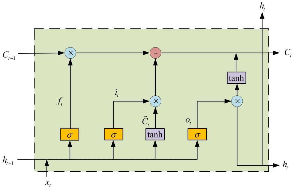
Figure 1 Structure of the LSTM model.

The variable C_t-1 represents the cell state in the LSTM. LSTM uses a forget gate to forget useless information. The expression is as shown in Equation (1):

$\begin{array}{ll}{f}_t=\sigma (W_f·[h_{t-1},x_t]+b_f)& (1)\end{array}$

where f_t represents the forget gate, W_f represents the weight matrix, b_f represents the bias vector, h_t-1 represents the output at the previous time step, x_t represents the input at the current time step, $\sigma$ represents a commonly used function in neural networks.

Next, information will be selectively processed using the input gate. It is expressed as shown in Equations (2) and (3):

$\begin{array}{ll}{i}_t=\sigma (W_i·[h_{t-1},x_t]+b_i)& (2)\end{array}$

$\begin{array}{ll}{C}_t=\text{tanh}(W_c·[h_{t-1},x_t]+b_c)& (3)\end{array}$

where $i_t$ represents the input gate, $W_i$ and $W_c$ represent the weight matrix of the input gate, $b_i$ and $b_c$ represent the bias vector of the input gate, while $C_t$ denotes the current input unit’s state.

Subsequently, the cell state is updated as shown in Equation (4):

$\begin{array}{ll}{C}_t=f_t\times C_{t-1}+i\times {\tilde{C}}_t& (4)\end{array}$

Finally, the information is selected to be carried to the next neuron through the output gate, as shown in Equations (5) and (6):

$\begin{array}{ll}{o}_t=\sigma (W_o[h_{t-1},x_t]+b_o)& (5)\end{array}$

$\begin{array}{ll}{h}_t=o_t\times \tanh (C_t)& (6)\end{array}$

where o_t represents the output gate, $W_o$ represents the weight matrix of the output gate, b_o represents the bias vector of the output gate.

It is through the combination of these gates that important information in LSTM is preserved while irrelevant information is discarded. However, there are limitations to this approach. The performance of LSTM is poor when dealing with non-stationary time series data (Hao et al., 2022; Zhao et al., 2023).

2.2 Variational mode decomposition (VMD)

VMD is a decomposition method for complex signals. Significant wave height as a non-stationary time series is suitable for decomposition by VMD. VMD effectively converts the process of decomposition into an optimization process, which involves solving a variational problem. Building the variational problem and solving it are the two main parts of VMD. Variational mode refers to the mode obtained by solving the variational problem. VMD iteratively searches for the optimal solution of the variational mode and is capable of adaptively updating the optimal center frequency and bandwidth of each Intrinsic Mode Function (IMF) (Dragomiretskiy and Zosso, 2013).

VMD has redefined the intrinsic mode functions as given in Equation (7):

$\begin{array}{ll}{u}_k(t)=A_k(t)\cos ({\varphi }_k(t))& (7)\end{array}$

where k is the mode number, $A_k(t)$ is the amplitude of the k mode, ${\varphi }_k(t)$ is the phase of the k mode, $u_k(t)$ is the k mode function.

The constrained variational problem that has been framed is as shown in Equation (8):

$\begin{array}{ll}\{\begin{array}{c}\min {}_{\left\{u_k\right\}\left\{{\overline{\omega }}_k\right\}}\left\{\sum _{k=1}^K{\Vert {\partial }_t\left[\left(\delta (t)+\frac{j}{\pi t}\right)\ast u_k(t)\right]e^{-j{\overline{\omega }}_{k}t}\Vert }_2^2\right\}\\ \text{ s}.\text{t}.\sum _{k=1}^K{u}_k(t)=f\end{array}& (8)\end{array}$

where $u_k$ represents the respective mode functions, while ${\overline{\omega }}_k$ represents the respective mode center frequencies.

A transformation of the constrained variational problem into an unconstrained variational problem is performed in order to solve the constrained optimization issue that was referenced before. The introduction of an enhanced Lagrangian function is accomplished by using the advantages of quadratic penalty terms and the Lagrange multiplier approach, as shown in Equation (9) (Bertsekas, 1976).

$\begin{array}{ll}\begin{array}{l}L\left(\left\{u_k\right\},\left[{\overline{\omega }}_k\right\},\lambda \right)=\alpha \sum _{k=1}^K{\Vert {\partial }_t\left[\left(\delta (t)+\frac{j}{\pi t}\right)\ast u_k(t)\right]e^{-j{\overline{\omega }}_{k}t}\Vert }_2^2\hfill \\ +{\Vert f(t)-{\displaystyle \sum _{k=1}^K}{u}_k(t)\Vert }_2^2+\langle \lambda (t),f(t)-\sum _{k=1}^K{u}_k(t)\rangle \hfill \end{array}& (9)\end{array}$

where α represents the variance regularization parameter, while λ represents the Lagrangian multiplier.

To address the aforementioned variational problem, alternating direction method of multipliers (ADMM) is employed (Hestenes, 1969). The procedure is outlined as follows:

1. Initialize $u_k^1,{\overline{\omega }}_k^1,{\lambda }_k^1$ and n.

2. The value of the variable n is increased by one, and then the program moves on to the loop.

3. Based on Equation (10), it is seen that the variables $u_k$ and ${\overline{\omega }}_k$ undergo modifications. At the point when the number of iterations exceeds k, the process of updating comes to an end.

$\begin{array}{ll}\{\begin{array}{c}{\widehat{u}}_k^{n+1}(\omega )=\frac{\widehat{f}(\omega )-{\sum }_{i<k}{\widehat{u}}_i^{n+1}(\omega )+{\sum }_{i>k}{\widehat{u}}_i^n(\omega )+\frac{{\widehat{\lambda }}^n(\omega )}{2}}{1+2\alpha {(\omega -{\overline{\omega }}_k^n)}^2}\\ {\overline{\omega }}_k^{n+1}=\frac{{\int }_0^{\infty }\omega {\left|{\widehat{u}}_k^{n+1}(\omega )\right|}^{2}d\omega }{{\int }_0^{\infty }{\left|{\widehat{u}}_k^{n+1}(\omega )\right|}^{2}d\omega }\end{array}& (10)\end{array}$

4. According to Equation (11), the variable λ is updated.

$\begin{array}{ll}{\widehat{\lambda }}^{n+1}(\omega )={\widehat{\lambda }}^n(\omega )+\tau \left(\widehat{f}(\omega )-\sum _{k=1}^K{\widehat{u}}_k^{n+1}(\omega )\right)& (11)\end{array}$

5. In the event that the user-defined variable ϵ fulfills the stopping requirement as shown in Equation (12), the loop is ended. If it does not satisfy the condition, the loop carries on to step 2 and continues the iteration.

$\begin{array}{ll}\sum _{k=1}^K\frac{{\Vert {\widehat{u}}_k^{n+1}(\omega )-{\widehat{u}}_k^n(\omega )\Vert }_2^2}{{\Vert {\widehat{u}}_k^n(\omega )\Vert }_2^2}<\epsilon & (12)\end{array}$

By constructing and solving the variational problem, VMD can effectively decompose non-stationary data. However, the mode number k after the decomposition by VMD needs to be chosen artificially. In order to find the most suitable mode number k, many tests are required.

2.3 VMD-LSTM-direct

The traditional direct decomposition is to generate the subsequences by directly decomposing all the data using VMD. Suppose there are m data in total. The first k data are classified as a training set, and the last m-k data are classified as a testing set. The process of direct decomposition is shown in Figure 2. It should be emphasized that this prediction uses an ensemble prediction architecture, where the input to the LSTM model is the decomposed subsequences, and the output of the LSTM model is significant wave height. The prediction architecture is applied to fully reflect the relationship between the subsequences. The final prediction is obtained from the trained LSTM model. The whole process is illustrated in Figure 3. It should be noted that the direct decomposition contains the data of the unknown testing set. In other words, information leakage occurs when the original data is decomposed using knowledge about future values that is not known. Due to the leakage of future information, the high model accuracy is unreliable, and the laws of time series prediction are deviated (Wang and Wu, 2016).

Figure 2

Figure 2 Traditional decomposition process.

Figure 3

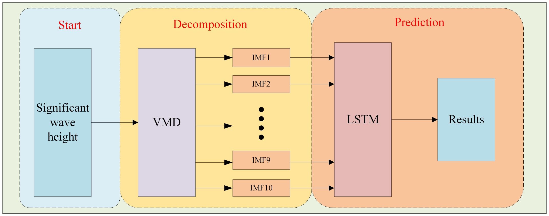
Figure 3 Flow chart of the hybrid VMD-LSTM-direct significant wave height prediction model.

2.4 VMD-LSTM-rolling

Rolling decomposition is a method that differs from traditional direct decomposition. Suppose there are m data in total. The first k data are classified as a training set, and the last m-k data are classified as a testing set. The process of rolling decomposition is presented in Figure 4. Time series are generated by a rolling method, after which each time series is decomposed. Rolling decomposition and the VMD-LSTM-rolling model are described below:

1. First, the first k data are considered as time series 1, which are decomposed using VMD to get the subsequences. It should be emphasized that this prediction uses an ensemble prediction architecture, where the input to the LSTM model is the decomposed subsequences, and the output of the LSTM model is significant wave height. Using the trained LSTM model, the prediction at the moment k+1 is obtained, denoted as prediction1.

2. Next, consider the actual data at the moment k+1 as known data. At this point, the first data to the k+1th data are regarded as time series 2. Just like step 1, the time series 2 is decomposed using VMD to get the subsequences, and then the subsequences are used as the input to the LSTM model, and significant wave height is used as the output of the LSTM model. The trained LSTM model is used to get the prediction at the moment k+2, denoted as prediction2.

3. Continue executing the aforementioned procedures until the rolling decomposition and the prediction processes have been finished. The prediction1, prediction2,…, and predictionn are the prediction results corresponding to the testing set. Then all the predictions are combined together to form the final results. It should be noted that all the predictions are combined together rather than being added up. The complete procedure is depicted in Figure 5.

Figure 4

Figure 4 The proposed rolling decomposition process.

Figure 5

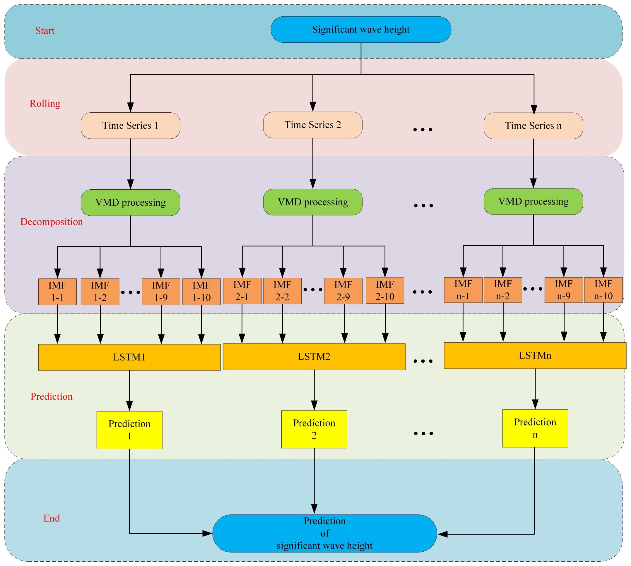
Figure 5 Flow chart of the hybrid VMD-LSTM-rolling significant wave height prediction model.

With the designed rolling decomposition and ensemble prediction architecture, predictions are made for only one testing set data at a time. When predicting the next testing set data, the current testing set data is considered known. This design maximizes the use of all available data for the purpose of learning. It is crucial to emphasize that the actual value of the first testing set data, rather than the predicted value, is added. This is because the actual value of the first testing set data is considered known after prediction, and the model becomes more stable by adding the actual value.

We need to emphasize that for multi-step prediction we use a static prediction approach (Fu et al., 2023). For example, in the four-step-ahead prediction, we predict significant wave height at hour 11 using 1–7 h of data.

2.5 Persistence forecast (PF)

PF is a very simple prediction method, which uses significant wave height of the previous hours as the prediction for this hour (Rasp et al., 2020). It can be expressed by Equation (13):

$\begin{array}{ll}\text{Hs }(\text{t}+\text{k})=\text{Hs}(\text{t})& (13)\end{array}$

where Hs(t) represents significant wave height of the previous hours, and Hs(t + k) represents prediction for this hour.

If the model’s prediction is worse than the PF, the model’s performance is not satisfactory.

2.6 Evaluation metrics

For the purpose of evaluating the model’s performance, this study uses four metrics to quantify the discrepancies between the actual and predicted values, namely R², MAE, RMSE and MAPE. R² is used to quantify the degree of agreement. MAE is the mean of the absolute errors. RMSE is used to quantify the average difference. MAPE is the percentage version of relative errors. The formulas are as stated in Equations (14)–(17):

$\begin{array}{ll}{R}^2=1-\frac{{\sum }_{i=1}^n{({\widehat{y}}_i-y_i)}^2}{{\sum }_{i=1}^n{({\overline{y}}_i-y_i)}^2}& (14)\end{array}$

$\begin{array}{ll}MAE=\frac{1}{n}{\sum }_{i=1}^n\left|y_i-{\widehat{y}}_i\right|& (15)\end{array}$

$\begin{array}{ll}RMSE=\sqrt{\frac{1}{n}{\displaystyle \sum _{i=1}^n}{(y_i-{\widehat{y}}_i)}^2}& (16)\end{array}$

$\begin{array}{ll}MAPE=\frac{100\%}{n}\sum _{i=1}^n\left|\frac{{\widehat{y}}_i-y_i}{y_i}\right|& (17)\end{array}$

where ${\widehat{y}}_i$ represents the predicted value, $y_i$ represents the actual value, ${\overline{y}}_i$ represents the mean of the actual values, and n represents the number of data samples.

In addition, this study employs Taylor diagrams to assess the accuracy of the model (Taylor, 2001). The common Taylor diagram accuracy indicators used in this study are correlation coefficient R, The standard deviation STD, and the centered root-mean-square difference E′. The formulas are as stated in Equations (18)–(20):

$\begin{array}{ll}R=\frac{{\sum }_{i=1}^n(y_i-{\overline{y}}_i)({\widehat{y}}_i-{\overline{\widehat{y}}}_i)}{\sqrt{{\sum }_{i=1}^n{(y_i-{\overline{y}}_i)}^2·{\sum }_{i=1}^n{({\widehat{y}}_i-{\overline{\widehat{y}}}_i)}^2}}& (18)\end{array}$

$\begin{array}{ll}STD=\sqrt{\frac{1}{n}{\displaystyle \sum _{i=1}^n}{(x_i-\overline{x})}^2}& (19)\end{array}$

$\begin{array}{ll}{E}^{\prime }={\left\{\frac{1}{n}{\displaystyle \sum _{i=1}^n}{\left[\left(y_i-{\overline{y}}_i\right)-\left({\widehat{y}}_i-{\overline{\widehat{y}}}_i\right)\right]}^2\right\}}^{1/2}& (20)\end{array}$

where ${\widehat{y}}_i$, $y_i$, ${\overline{y}}_i$ and n have explained above. ${\overline{\widehat{y}}}_i$ represents the mean of the predicted values. $x_i$ and $\overline{x_i}$ represents the value and the mean value of the sequence which is used to calculate STD.

2.7 Neural network design

First, the dataset partitioning should be emphasized. The dataset was partitioned into two subsets: a training set including the initial 90% of the data, consisting of 4008 samples, and a testing set comprising the last 10%, consisting of 408 samples.

The accuracy of neural networks can be achieved by increasing the layers, but deepening the layers will significantly increase the computation time (Pfeiffenberger and Bates, 2018). The experiment was conducted in a Python 3.7 environment and used the Keras module of TensorFlow 2.10.0 to build the LSTM model. Based on previous experience and multiple experiments, the LSTM model was divided into 5 layers: an input layer, three hidden layers, and an output layer. The first hidden layer, the second hidden layer and the third hidden layer consisted of 128, 64 and 32 neurons, respectively. Dropout was set to 0.2. The MSE was chosen as the loss function, and the Adam optimizer was used. A total of 100 epochs were set up, with a batch size of 32. Early stopping was implemented with a patience of 10 to avoid overfitting. The timestep was set to 7, which meant that the significant wave height of the current hour was considered to be related to the previous seven hours.

3 Wave datasets preprocessing

3.1 Research area

This study was conducted in the South Sea of China. Two positions were selected. The coordinates of position 1 were (21.50°N,113.00°E), and the coordinates of position 2 were (23.00°N,117.00°E). Figure 6 illustrates the location of the position that was chosen for this study. The data used for prediction were obtained from ERA5 of the European Centre for Medium-Range Weather Forecasts (ECMWF) and covered the period from July 1, 2018, 0:00 UTC to December 31, 2018, 23:00 UTC. A total of 4416 valid data were included in the analysis. The dataset1 and the dataset2 used in this paper are presented in Figures 7, 8, respectively.

Figure 6

Figure 6 Distribution of the selected position in the South Sea of China.

Figure 7

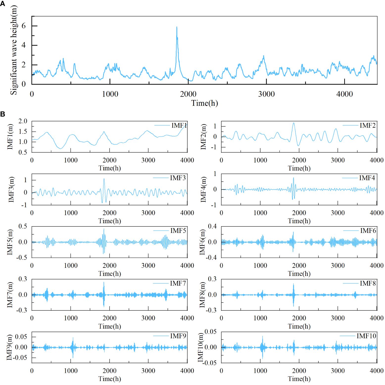
Figure 7 Significant wave height and decomposition results of time series 1 for dataset1 (A) significant wave height, (B) decomposition results of time series 1.

Figure 8

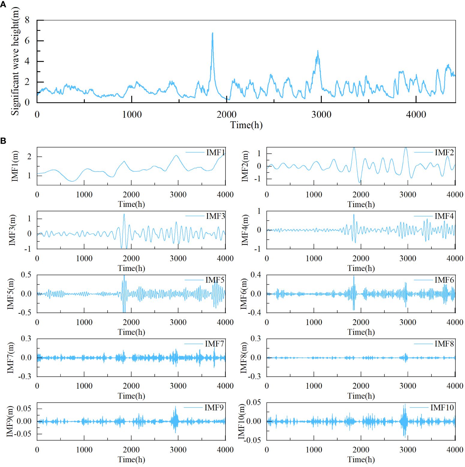
Figure 8 Significant wave height and decomposition results of time series 1 for dataset2 (A) significant wave height, (B) decomposition results of time series 1.

We need to emphasize the reason why we did not select longer significant wave height data. The rolling decomposition method, which is equivalent to constructing multiple LSTM models for training, greatly increases the training time compared to direct decomposition. If the data length is too long, the training time will be too large. Therefore, we used this time period to conduct our study.

3.2 Data processing

The value of k has a substantial influence on the VMD decomposition, which was determined to be 10 in this study based on previous experience and multiple experiments (Zhou et al., 2022; Zhao et al., 2023). Due to space constraints, only the decomposition results of time series 1 for dataset1 and dataset2 are exhibited here. As shown in Figures 7, 8, the time series 1 is decomposed into 10 IMF components. After being decomposed by VMD, the dataset becomes stationary.

4 Results and discussion

4.1 Multi-step prediction results by different models

Tables 1, 2 record the error statistics of multi-step predictions by different models. Figure 9 shows comparison of the statistical results of twelve-step-ahead prediction using Taylor diagrams. Figures 10, 11 present the multi-step prediction results by different models. “1h” in Figures 10, 11 represents December 15, 2018, at 00:00 UTC. Figures 12, 13 depict scatter plots of measurements and predictions by the LSTM model and the VMD-LSTM-rolling model. The closer the best-fit slope is to 1, the better the fitting effect.

Table 1

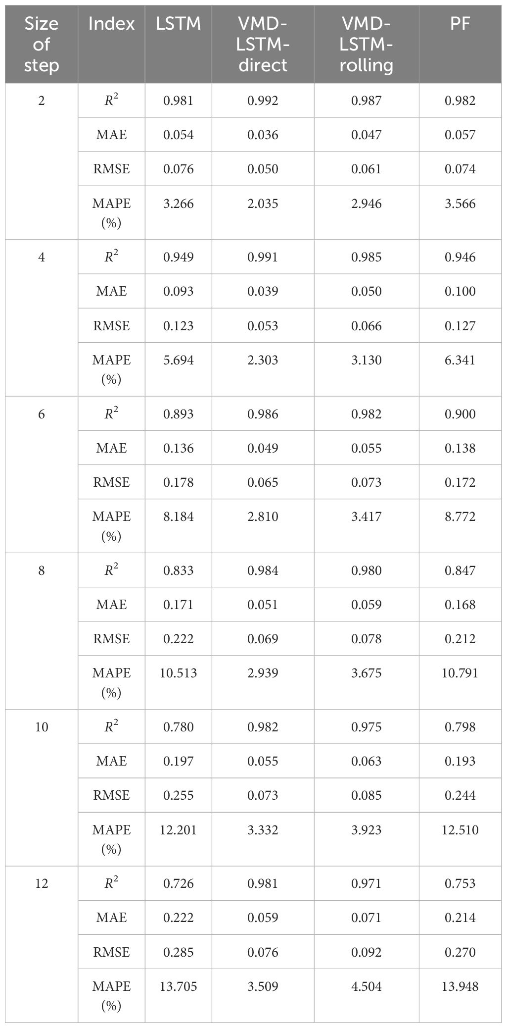
Table 1 Error measures of multi-step predictions of dataset1 by different models.

Table 2

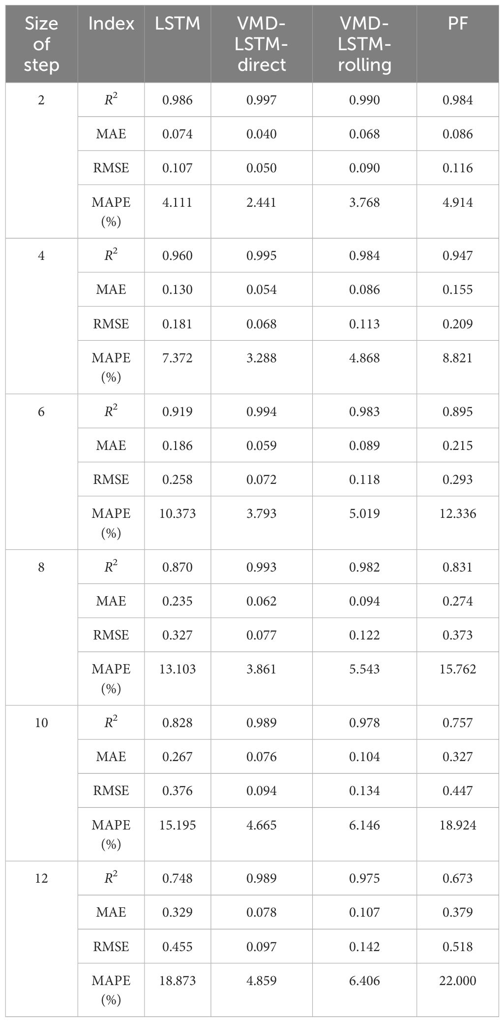
Table 2 Error measures of multi-step predictions of dataset2 by different models.

Figure 9

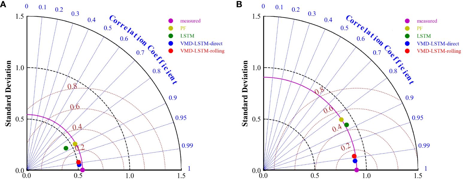
Figure 9 Comparison of the statistical results using Taylor diagrams (A) dataset1, (B) dataset2.

Figure 10

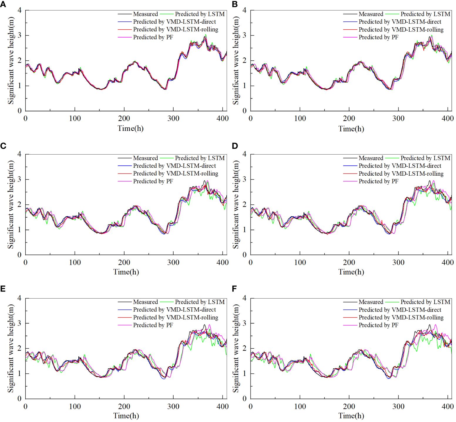
Figure 10 Predictions of significant wave height of dataset1 by different models for several future hours (A) 2 hours, (B) 4 hours, (C) 6 hours, (D) 8 hours, (E) 10 hours and (F) 12 hours.

Figure 11

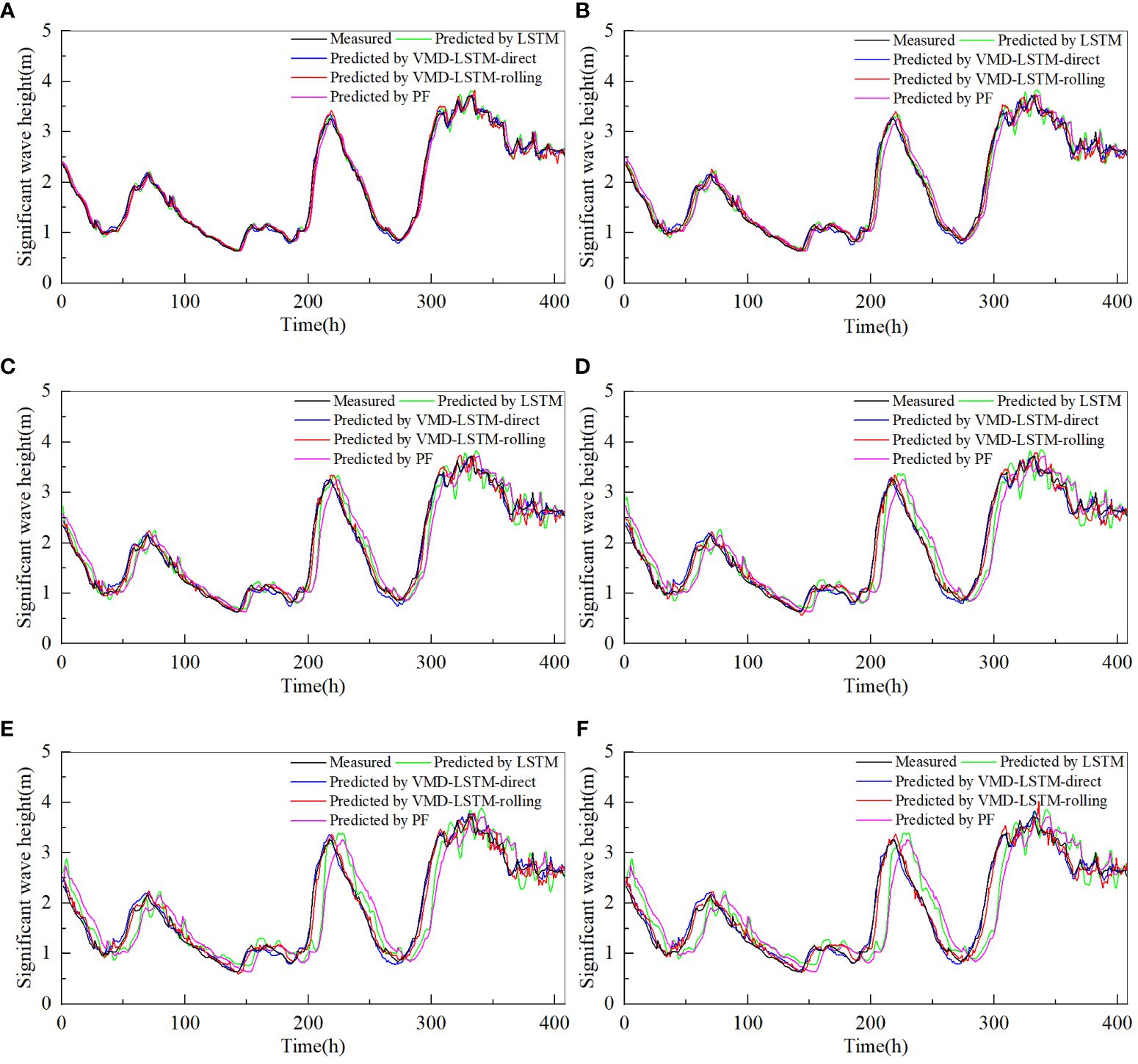
Figure 11 Predictions of significant wave height of dataset2 by different models for several future hours (A) 2 hours, (B) 4 hours, (C) 6 hours, (D) 8 hours, (E) 10 hours and (F) 12 hours.

Figure 12

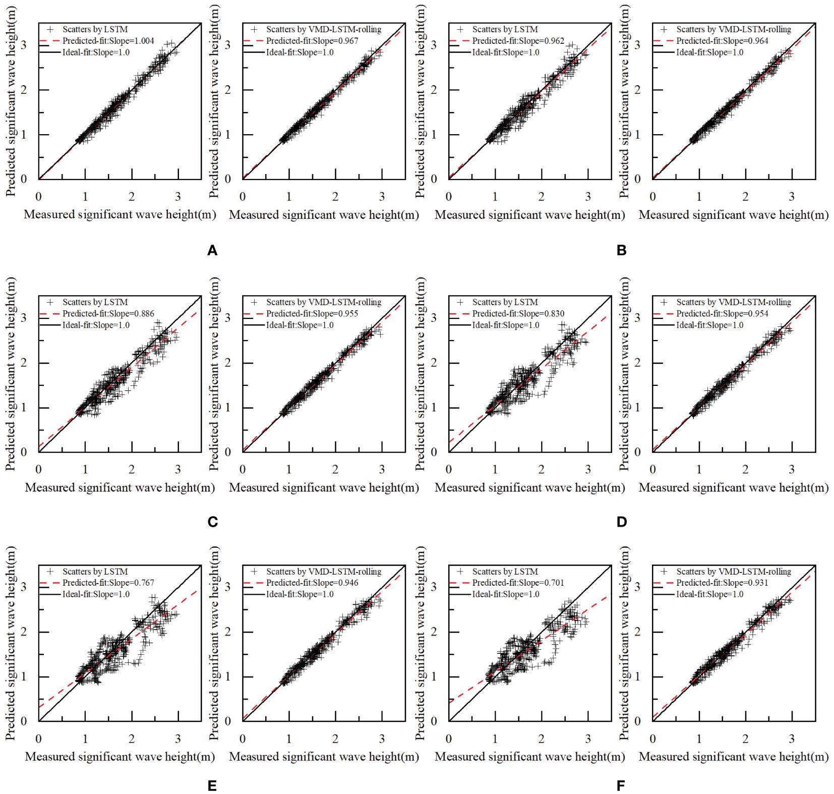
Figure 12 Scatter diagram of the measurements and predictions of dataset1 by different models for several future hours (A) 2 hours, (B) 4 hours, (C) 6 hours, (D) 8 hours, (E) 10 hours and (F) 12 hours.

Figure 13

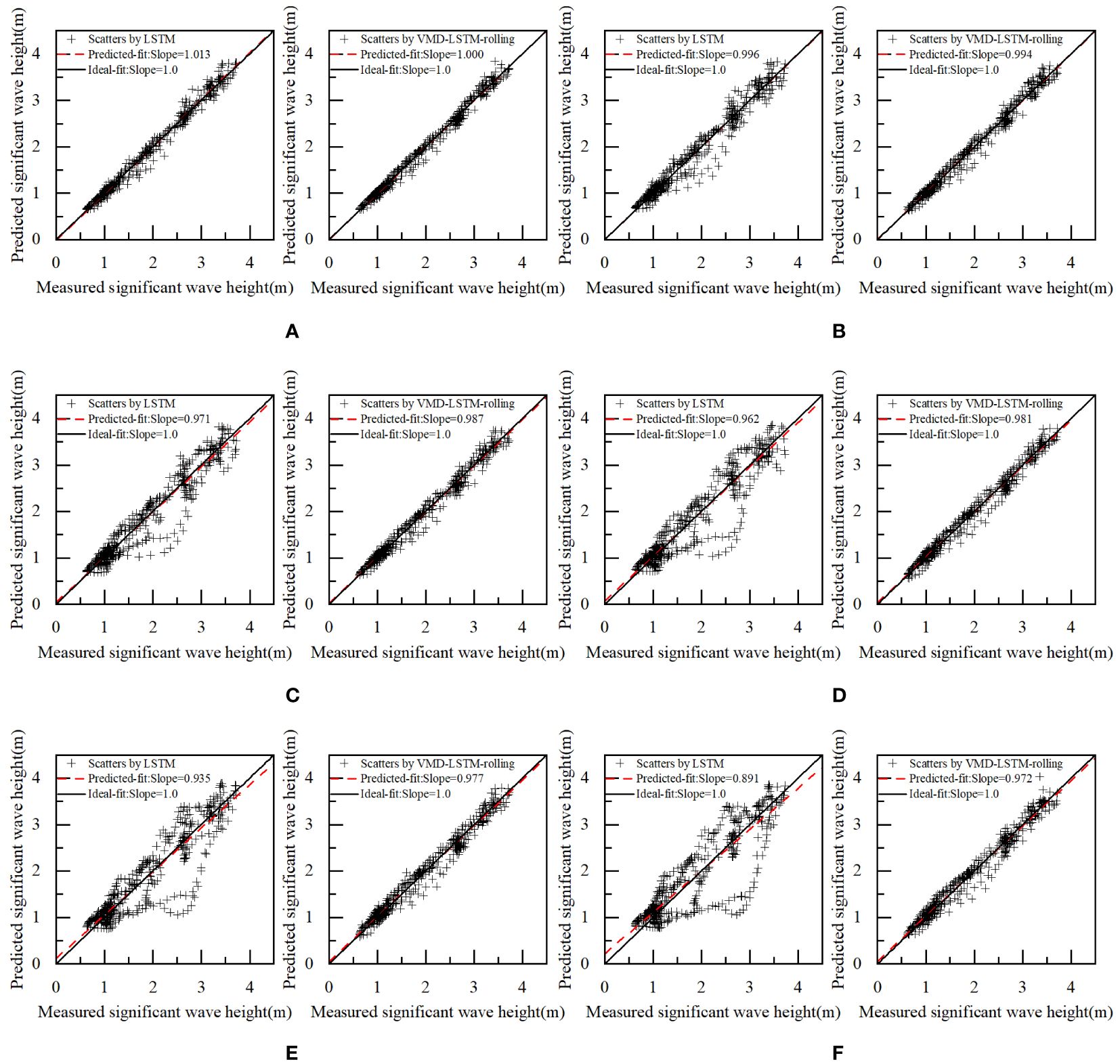
Figure 13 Scatter diagram of the measurements and predictions of dataset2 by different models for several future hours (A) 2 hours, (B) 4 hours, (C) 6 hours, (D) 8 hours, (E) 10 hours and (F) 12 hours.

4.2 Discussion of the prediction results

From Tables 1, 2, it can be seen that the prediction results by the LSTM model are in good agreement with the actual values for the small step-ahead prediction. When the number of prediction steps is two, R², MAE, RMSE and MAPE of prediction results by the LSTM model are 0.981, 0.054, 0.076 and 3.266% respectively for dataset1, which indicates that there is only a minor discrepancy between the predicted results and the actual results. All evaluation metrics of the LSTM model exceed PF for dataset2, while the evaluation metrics of the LSTM model has its own advantages and disadvantages compared to PF for dataset1. Overall, the performance of the LSTM model is satisfactory. Observing Figures 10, 11, it is noticeable that the LSTM model can accurately capture the trend of the original significant wave height, and the prediction results at the peaks and troughs align closely with actual values. The phase shift of the LSTM model is very small and close to PF. The high prediction accuracy demonstrates that the LSTM model has a strong ability to deal with non-linear problems and is suitable for the small step-ahead prediction.

However, as the prediction duration increases, the error of the LSTM model grows rapidly. As can be seen from Tables 1, 2, for the twelve-step-ahead prediction, R² of prediction results by the LSTM model is only 0.726, while MAE, RMSE and MAPE surge to 0.222, 0.285 and 13.705% respectively for dataset1, which means that the prediction results are inaccurate. The accuracy of the LSTM model is still higher than PF for dataset2. However, the performance of the LSTM model is worse compared to PF for dataset1, which demonstrates that the prediction results of the LSTM model are poor. As shown in Figures 10, 11, the phase shifts of the LSTM model are quite similar to PF. As the prediction duration increases, the prediction results exhibit noticeable phase shifts from the measured curve. The larger the number of prediction steps, the more noticeable the phase shift becomes. The occurrence of this phenomenon may be attributed to the non-stationarity of significant wave height. The effect of non-stationarity is not apparent when the number of prediction steps is not large but becomes more pronounced as the number of prediction steps grows. Hao et al. (2022) observed the phase shift when using the LSTM model to predict significant wave height, which aligns with the findings of this study. It is evident that when the number of prediction steps is large, the LSTM model fails to fulfill the requirements of significant wave height prediction.

The VMD-LSTM-direct model and the VMD-LSTM-rolling model overcome this drawback by decomposing the original data into 10 IMFs through the VMD algorithm, improving the stationarity of the data. As can be seen from Tables 1, 2, even with a small number of prediction steps, both the VMD-LSTM-direct model and the VMD-LSTM-rolling model already outperform the LSTM model in terms of prediction accuracy. As the prediction duration increases, this improvement becomes more greater. For twelve-step-ahead prediction, R² of the prediction results by the VMD-LSTM-direct model for dataset1 is improved by 35.09% compared to the LSTM model, while MAE, RMSE and MAPE are decreased by 73.55%, 73.37% and 74.40%, respectively. R² of the prediction results by the VMD-LSTM-rolling model for dataset1 is improved by 33.82% compared to the LSTM model, while MAE, RMSE and MAPE are decreased by 67.97%, 67.67% and 67.14%, respectively. All evaluation metrics of the VMD-LSTM-direct model and the VMD-LSTM-rolling model are substantially ahead of PF. It can be seen very clearly that both the VMD-LSTM-direct model and the VMD-LSTM-rolling model achieve more accurate results. Even with a large number of prediction steps, the prediction results still maintain a high accuracy.

We visualize statistical results through Taylor diagrams. Twelve-step statistical results are plotted in Figure 9. The colored scatter in the Taylor diagrams represents the model. The blue line, the black line and the brown line represent the correlation coefficient R, the standard deviation STD and the centered root-mean-square difference E′, respectively. It can be clearly seen that the LSTM model and PF are far away from the measured value, which means that the LSTM model and PF have the poor prediction performance. In comparison, the VMD-LSTM-direct model and the VMD-LSTM-rolling model are quite close to the measured value, which indicates that the accuracy of the VMD-LSTM-direct model and the VMD-LSTM-rolling model are substantially improved compared to the LSTM model and PF.

From Figures 10, 11, it can be seen that both the VMD-LSTM-direct model and the VMD-LSTM-rolling model are able to capture the characteristics and the general trend of the original significant wave height. At the same time, the phase shifts of the VMD-LSTM-direct model and the VMD-LSTM-rolling model are much smaller than the LSTM model and PF. The reduction of the phase shift is an important reason why the prediction error can be decreased. Both the VMD-LSTM-direct model and the VMD-LSTM-rolling model retain the ability to deal with non-linear problems, therefore they achieve excellent performance in short-term prediction. In addition, the impact of non-stationarity caused by significant wave height is effectively suppressed due to VMD decomposition, which plays a vital role in the improvement of long-term prediction accuracy. It is obvious that both the VMD-LSTM-direct model and the VMD-LSTM-rolling model exhibit an obvious superiority in the domain of prediction compared to the LSTM model and PF, especially for large step-ahead prediction.

As shown in Tables 1, 2, the accuracy of direct decomposition is higher than rolling decomposition. Additionally, the VMD-LSTM-direct model is closer to the measured value than the VMD-LSTM-rolling model in Figure 9.The reason for this phenomenon is that when decomposing the data for the VMD-LSTM-direct model, the training set together with the testing set is decomposed, which is not reasonable. The testing set is unknown, so this decomposition approach leaks the future data and gets the features of the future data, which improves the accuracy of prediction. However, direct decomposition is impossible to be applied in real life and can lead to false accuracy. Rolling decomposition is different because it ensures that no future data is leaked by only decomposing known data. Although the accuracy of rolling decomposition is lower than direct decomposition, rolling decomposition ensures the veracity of the prediction results and the feasibility of the method in real life, which is more correct.

Considering that the direct decomposition method cannot be applied in real life, the VMD-LSTM-direct model will not be included in the following discussion. Observing Figures 12, 13, it is clear that there is a severe divergence between the prediction results by the LSTM model and the actual values as the prediction duration increases. For the twelve-step-ahead prediction, the best-fit slopes of the LSTM model are only 0.701 for dataset1 and 0.891 for dataset2. This situation is substantially improved after using the rolling decomposition, which suppresses the error caused by the non-stationarity of the original significant wave height. Although the increase in prediction steps leads to a slight decrease in the best-fit slopes, the decrease is minimal. It can be clearly seen that when the number of prediction steps is twelve, the best-fit slopes of the VMD-LSTM-rolling model are 0.931 for dataset1 and 0.972 for dataset2, which implies that the prediction results are very close to the actual values. The analysis leads to the conclusion that the VMD-LSTM-rolling model has obvious advantages in prediction, especially when the number of prediction steps is large because using rolling decomposition improves the stationarity of significant wave height. Meanwhile, the rolling decomposition can also take into account the realistic use without the problem of future leakage.

5 Conclusion

The non-stationarity is a critical factor that strongly influences the accurate prediction of significant wave height. The impact of non-stationarity is amplified as the prediction duration increases. For the small step-ahead prediction, the LSTM model can still obtain accurate results. However, as the prediction duration increases, the accuracy of the LSTM model significantly decreases, and phase shift starts to occur. Data decomposition methods are applied in order to improve the prediction accuracy. However, improper decomposition model will lead to information leakage. To address this issue, we propose a model called rolling decomposition.

In this paper, the significant wave height data in the South China Sea were obtained from ERA5 of the ECMWF. The LSTM model, the VMD-LSTM-direct model and the VMD-LSTM-rolling model were built to predict significant wave height. Then the performance of these models were compared. After comparison, the following findings were made:

In multi-step prediction, the LSTM model exhibits phase shift due to the non-stationarity of significant wave height. The magnitude of the shift increases with the number of prediction steps. To address this issue, the VMD-LSTM-direct model and the VMD-LSTM-rolling model decompose the significant wave height by the VMD algorithm and obtain stationary IMFs, which drastically mitigates the phase shift problem. Meanwhile, the VMD-LSTM-direct model and the VMD-LSTM-rolling model significantly reduce the prediction errors and achieve excellent performance in both short-term and long-term prediction. These phenomena indicate that the VMD-LSTM-direct model and the VMD-LSTM-rolling model possess the capability to handle non-stationary data.

The VMD-LSTM-direct model decomposes all data, obtaining the features of the future data, so the accuracy exceeds that of the VMD-LSTM-rolling model. However, the VMD-LSTM-direct model leaks the information of the testing set, which makes it impossible to be applied in practice. Rolling decomposition ensures no leakage of future data by only decomposing known data. Therefore, rolling decomposition is more correct and can be used in real life.

In summary, the proposed rolling decomposition model not only significantly improves the prediction accuracy of the LSTM model but also successfully avoids the issue of information leakage. The rolling decomposition model can accurately predict significant wave height, demonstrating strong practical significance and application value.

Although the proposed rolling decomposition model achieves good accuracy, it still leaves questions for us to ponder. We only use significant wave height to build the model while other parameters are not incorporated into our prediction model. Whether or not adding other parameters would improve the model is a topic we will experiment with in the future. Besides, only one data decomposition method VMD is used in the model. In future research, rolling decomposition based on other data decomposition methods will be explored.

Data availability statement

The raw data supporting the conclusions of this article will be made available by the authors, without undue reservation.

Author contributions

TD: Writing – original draft, Software, Methodology, Conceptualization. DW: Writing – review & editing, Supervision, Funding acquisition. LS: Writing – review & editing, Validation, Investigation. QL: Writing – review & editing, Supervision, Software, Data curation. XZ: Writing – review & editing, Validation, Software, Methodology. YL: Writing – review & editing, Validation, Data curation.

Funding

The author(s) declare financial support was received for the research, authorship, and/or publication of this article. The present work is sponsored by the National Natural Science Foundation of China (Grant No.42176166; No.41776024), National Key Research and Development Program of China (No.2024YFE0101000) and Major Project of Power Construction Corporation of China, Ltd (DJ-ZDXM-2022–28; KJXMWW-2023–01).

Acknowledgments

The significant wave height used is sourced from ERA5 of the ECMWF. We would like to acknowledge the ECMWF.

Conflict of interest

Authors LS and YL were employed by Municipal Engineering Corporation Limited. Authors QL and XZ were employed by Power China Kunming Engineering Corporation Limited.

The remaining authors declare that the research was conducted in the absence of any commercial or financial relationships that could be construed as a potential conflict of interest.

The authors declare that this study received funding from Power Construction Corporation of China, Ltd. The funder had the following involvement in the study: study design, data collection and analysis, and preparation of the manuscript.

Publisher’s note

All claims expressed in this article are solely those of the authors and do not necessarily represent those of their affiliated organizations, or those of the publisher, the editors and the reviewers. Any product that may be evaluated in this article, or claim that may be made by its manufacturer, is not guaranteed or endorsed by the publisher.

References

Ahn S., Neary V. S., Allahdadi M. N., He R. (2021). Nearshore wave energy resource characterization along the east coast of the United States. Renewable Energy 172, 1212–1224. doi: 10.1016/j.renene.2021.03.037

CrossRef Full Text | Google Scholar

Amunugama M., Suzuyama K., Manawasekara C., Tanaka Y., Xia Y. (2020). Typhoon-induced storm surge analysis with coawst on different modelled forcing. J. Japan Soc. Civil Engineers Ser. B3 (Ocean Engineering) 76, I_210–I_215. doi: 10.2208/jscejoe.76.2_I_210

CrossRef Full Text | Google Scholar

Bertsekas D. P. (1976). Multiplier methods: A survey. Automatica 12, 133–145. doi: 10.1016/0005-1098(76)90077-7

CrossRef Full Text | Google Scholar

Bethel B. J., Sun W., Dong C., Wang D. (2022). Forecasting hurricane-forced significant wave heights using a long short-term memory network in the caribbean sea. Ocean Sci. 18, 419–436. doi: 10.5194/os-18-419-2022

CrossRef Full Text | Google Scholar

Booij N., Ris R. C., Holthuijsen L. H. (1999). A third-generation wave model for coastal regions: 1. model description and validation. J. geophysical research: Oceans 104, 7649–7666. doi: 10.1029/98JC02622

CrossRef Full Text | Google Scholar

Bouke M. A., Abdullah A. (2023). An empirical study of pattern leakage impact during data preprocessing on machine learning-based intrusion detection models reliability. Expert Syst. Appl. 230, 120715. doi: 10.1016/j.eswa.2023.120715

CrossRef Full Text | Google Scholar

Cai X., Li D. (2024). M-edem: A mnn-based empirical decomposition ensemble method for improved time series forecasting. Knowledge-Based Syst. 283, 111157. doi: 10.1016/j.knosys.2023.111157

CrossRef Full Text | Google Scholar

Ding T., Wu D., Li Y., Shen L., Zhang X. (2024). A hybrid ceemdan-vmd-timesnet model for significant wave height prediction in the south sea of China. Front. Mar. Sci. 11. doi: 10.3389/fmars.2024.1375631

CrossRef Full Text | Google Scholar

Dragomiretskiy K., Zosso D. (2013). Variational mode decomposition. IEEE Trans. Signal Process. 62, 531–544. doi: 10.1109/TSP.2013.2288675

CrossRef Full Text | Google Scholar

Duan W.-y., Huang L.-m., Han Y., Huang D.-t. (2016). A hybrid emd-ar model for nonlinear and non-stationary wave forecasting. J. Zhejiang University-SCIENCE A 17, 115–129. doi: 10.1631/jzus.A1500164

CrossRef Full Text | Google Scholar

Fu Y., Ying F., Huang L., Liu Y. (2023). Multi-step-ahead significant wave height prediction using a hybrid model based on an innovative two-layer decomposition framework and lstm. Renewable Energy 203, 455–472. doi: 10.1016/j.renene.2022.12.079

CrossRef Full Text | Google Scholar

Gao R., Du L., Suganthan P. N., Zhou Q., Yuen K. F. (2022). Random vector functional link neural network based ensemble deep learning for short-term load forecasting. Expert Syst. Appl. 206, 117784. doi: 10.1016/j.eswa.2022.117784

CrossRef Full Text | Google Scholar

Hao W., Sun X., Wang C., Chen H., Huang L. (2022). A hybrid emd-lstm model for non-stationary wave prediction in offshore China. Ocean Eng. 246, 110566. doi: 10.1016/j.oceaneng.2022.110566

CrossRef Full Text | Google Scholar

Hestenes M. R. (1969). Multiplier and gradient methods. J. optimization Theory Appl. 4, 303–320. doi: 10.1007/BF00927673

CrossRef Full Text | Google Scholar

Hochreiter S., Schmidhuber J. (1997). Long short-term memory. Neural Comput. 9, 1735–1780. doi: 10.1162/neco.1997.9.8.1735

CrossRef Full Text | Google Scholar

Hu H., Wang L., Zhang D., Ling L. (2023). Rolling decomposition method in fusion with echo state network for wind speed forecasting. Renewable Energy 216, 119101. doi: 10.1016/j.renene.2023.119101

CrossRef Full Text | Google Scholar

Huang N. E., Shen Z., Long S. R., Wu M. C., Shih H. H., Zheng Q., et al. (1998). The empirical mode decomposition and the hilbert spectrum for nonlinear and non-stationary time series analysis. Proc. R. Soc. London. Ser. A: mathematical Phys. Eng. Sci. 454, 903–995. doi: 10.1098/rspa.1998.0193

CrossRef Full Text | Google Scholar

Janssen P. A. (2008). Progress in ocean wave forecasting. J. Comput. Phys. 227, 3572–3594. doi: 10.1016/j.jcp.2007.04.029

CrossRef Full Text | Google Scholar

Jiang H., Zhang Y., Qian C., Wang X. (2024). ). Comment on papers using machine learning for significant wave height time series prediction: Complex models do not outperform auto-regression. Ocean Model. 189, 102364. doi: 10.1016/j.ocemod.2024.102364

CrossRef Full Text | Google Scholar

Kapoor S., Narayanan A. (2023). Leakage and the reproducibility crisis in machine-learningbased science. Patterns 4. doi: 10.1016/j.patter.2023.100804

CrossRef Full Text | Google Scholar

Li K., Shen R., Wang Z., Yan B., Yang Q., Zhou X. (2023). An efficient wind speed prediction method based on a deep neural network without future information leakage. Energy 267, 126589. doi: 10.1016/j.energy.2022.126589

CrossRef Full Text | Google Scholar

Mahjoobi J., Mosabbeb E. A. (2009). Prediction of significant wave height using regressive support vector machines. Ocean Eng. 36, 339–347. doi: 10.1016/j.oceaneng.2009.01.001

CrossRef Full Text | Google Scholar

Makarynskyy O., Pires-Silva A., Makarynska D., Ventura-Soares C. (2005). Artificial neural networks in wave predictions at the west coast of Portugal. Comput. geosciences 31, 415–424. doi: 10.1016/j.cageo.2004.10.005

CrossRef Full Text | Google Scholar

Pfeiffenberger E., Bates P. A. (2018). Predicting improved protein conformations with a temporal deep recurrent neural network. PloS One 13, e0202652. doi: 10.1371/journal.pone.0202652

CrossRef Full Text | Google Scholar

Pirhooshyaran M., Snyder L. V. (2020). Forecasting, hindcasting and feature selection of ocean waves via recurrent and sequence-to-sequence networks. Ocean Eng. 207, 107424. doi: 10.1016/j.oceaneng.2020.107424

CrossRef Full Text | Google Scholar

Rasp S., Dueben P. D., Scher S., Weyn J. A., Mouatadid S., Thuerey N. (2020). Weatherbench: a benchmark data set for data-driven weather forecasting. J. Adv. Modeling Earth Syst. 12, e2020MS002203. doi: 10.1029/2020MS002203

CrossRef Full Text | Google Scholar

Reikard G., Robertson B., Bidlot J.-R. (2017). Wave energy worldwide: Simulating wave farms, forecasting, and calculating reserves. Int. J. Mar. Energy 17, 156–185. doi: 10.1016/j.ijome.2017.01.004

CrossRef Full Text | Google Scholar

Rosenblatt M., Tejavibulya L., Jiang R., Noble S., Scheinost D. (2024). Data leakage inflates prediction performance in connectome-based machine learning models. Nat. Commun. 15, 1829. doi: 10.1038/s41467-024-46150-w

CrossRef Full Text | Google Scholar

Sarker M. A. (2018). Numerical modelling of waves and surge from cyclone chapala, (2015) in the arabian sea. Ocean Eng. 158, 299–310. doi: 10.1016/j.oceaneng.2018.04.014

CrossRef Full Text | Google Scholar

Song T., Wang J., Huo J., Wei W., Han R., Xu D., et al. (2023). Prediction of significant wave height based on eemd and deep learning. Front. Mar. Sci. 10. doi: 10.3389/fmars.2023.1089357

CrossRef Full Text | Google Scholar

Taylor K. E. (2001). Summarizing multiple aspects of model performance in a single diagram. J. geophysical research: atmospheres 106, 7183–7192. doi: 10.1029/2000JD900719

CrossRef Full Text | Google Scholar

Vijayan L., Huang W., Ma M., Ozguven E., Ghorbanzadeh M., Yang J., et al. (2023). Improving the accuracy of hurricane wave modeling in gulf of Mexico with dynamically-coupled swan and adcirc. Ocean Eng. 274, 114044. doi: 10.1016/j.oceaneng.2023.114044

CrossRef Full Text | Google Scholar

Wang Y., Wu L. (2016). On practical challenges of decomposition-based hybrid forecasting algorithms for wind speed and solar irradiation. Energy 112, 208–220. doi: 10.1016/j.energy.2016.06.075

CrossRef Full Text | Google Scholar

Yan K., Li C., Zhao R., Zhang Y., Duan H., Wang W. (2023). Predicting the ammonia nitrogen of wastewater treatment plant influent via integrated model based on rolling decomposition method and deep learning algorithm. Sustain. Cities Soc. 94, 104541. doi: 10.1016/j.scs.2023.104541

CrossRef Full Text | Google Scholar

Yu L., Ma Y., Ma M. (2021). An effective rolling decomposition-ensemble model for gasoline consumption forecasting. Energy 222, 119869. doi: 10.1016/j.energy.2021.119869

CrossRef Full Text | Google Scholar

Zhang J., Xin X., Shang Y., Wang Y., Zhang L. (2023). Nonstationary significant wave height forecasting with a hybrid vmd-cnn model. Ocean Eng. 285, 115338. doi: 10.1016/j.oceaneng.2023.115338

CrossRef Full Text | Google Scholar

Zhao L., Li Z., Qu L., Zhang J., Teng B. (2023). A hybrid vmd-lstm/gru model to predict non-stationary and irregular waves on the east coast of China. Ocean Eng. 276, 114136. doi: 10.1016/j.oceaneng.2023.114136

CrossRef Full Text | Google Scholar

Zhou F., Huang Z., Zhang C. (2022). Carbon price forecasting based on ceemdan and lstm. Appl. Energy 311, 118601. doi: 10.1016/j.apenergy.2022.118601

CrossRef Full Text | Google Scholar

Zhou S., Xie W., Lu Y., Wang Y., Zhou Y., Hui N., et al. (2021). Convlstm-based wave forecasts in the south and east China seas. Front. Mar. Sci. 8. doi: 10.3389/fmars.2021.680079

CrossRef Full Text | Google Scholar