
95% of researchers rate our articles as excellent or good
Learn more about the work of our research integrity team to safeguard the quality of each article we publish.
Find out more
ORIGINAL RESEARCH article
Front. Mar. Sci. , 03 June 2024
Sec. Coastal Ocean Processes
Volume 11 - 2024 | https://doi.org/10.3389/fmars.2024.1381228
 Linta Rose1*
 Matthew J. Widlansky1,2*
 Xue Feng1
 Philip Thompson1,2
 Taylor G. Asher3
 Gregory Dusek4
 Brian Blanton5
 Richard A. Luettich Jr.3
 John Callahan4,6William Brooks4
 Analise Keeney4Jana Haddad4,6
 William Sweet4Ayesha Genz7
 Paige Hovenga8
 John Marra7Jeffrey Tilson5
Coastal water level information is crucial for understanding flood occurrences and changing risks. Here, we validate the preliminary version (0.9) of NOAA’s Coastal Ocean Reanalysis (CORA), which is a 43-year reanalysis (1979–2021) of hourly coastal water levels for the Gulf of Mexico and Atlantic Ocean (i.e., the Gulf and East Coast region, or GEC). CORA-GEC v0.9 was conducted by the Renaissance Computing Institute using the coupled ADCIRC+SWAN coastal circulation and wave model. The model uses an unstructured mesh of nodes with varying spatial resolution that averages 400 m near the coast and is much coarser in the open ocean. Water level variations associated with tides and meteorological forcing are explicitly modeled, while lower-frequency water level variations are included by dynamically assimilating observations from NOAA’s National Water Level Observation Network. We compare CORA to water level observations that were either assimilated or not, and find that the reanalysis generally performs better than a state-of-the-art global ocean reanalysis (GLORYS12) in capturing the variability on monthly, seasonal, and interannual timescales as well as the long-term trend. The variability of hourly non-tidal residuals is also shown to be well resolved in CORA when compared to water level observations. Lastly, we present a case study of extreme water levels and coastal inundations around Miami, Florida to demonstrate an application of CORA for studying flood risks. Our assessment suggests that NOAA’s CORA-GEC v0.9 provides valuable information on water levels and flooding occurrence from 1979–2021 in areas that are experiencing changes across multiple time scales. CORA potentially can enhance flood risk assessment along parts of the U.S. Coast that do not have historical water level observations.
Coastal flooding, exacerbated by rising sea levels, poses threats to communities and ecosystems, motivating the need for comprehensive data to inform protective measures. Inadequacies of existing observing networks underscore the necessity for more detailed water level datasets, which are vital for monitoring and mitigating the impacts of coastal flooding. Responding to this requirement, the National Oceanic and Atmospheric Administration (NOAA) recently sponsored a 43-year reanalysis of hourly water levels for the coastal U.S., which has preliminary output during 1979–2021 for the Gulf of Mexico and northwestern Atlantic Ocean (hereafter referred to as the Gulf and East Coasts, or GEC region). NOAA’s new reanalysis is named the Coastal Ocean Reanalysis (CORA). This paper assesses the ability of the preliminary version of CORA-GEC (i.e., version 0.9) as it relates to describing observed coastal water level variability at multiple timescales. Discussion is provided as to how the data assimilation strategy employed in CORA (see its description in Asher et al., 2019) may lead to an opportunity for improved assessment of flooding risk for the Gulf and East Coasts, and perhaps elsewhere.
Producing CORA-GEC v0.9 (CORA, hereafter) includes running a hydrodynamic model forced by tides and meteorological fields as well as assimilating observed water levels. This work was undertaken by the Renaissance Computing Institute (RENCI) at the University of North Carolina at Chapel Hill using the ADvanced CIRCulation (ADCIRC) model coupled with the Simulating WAves Nearshore (SWAN) model. ADCIRC is a two-dimensional barotropic ocean circulation model proficient in resolving tidal and meteorologically-driven ocean responses (Luettich and Westerink, 2004; Westerink et al., 2008). SWAN is a spectral wave model able to generate, propagate, and dissipate ocean wind waves and swells (Booij et al., 1999; Zijlema, 2010). The coupling mechanism between ADCIRC and SWAN facilitates information passing between the models about water levels and waves, as described in the next section.
The ADCIRC model operates on a dynamic finite-element unstructured-mesh framework, which allows the spatial resolution to be variable. Its domain encompasses the northwestern Atlantic Basin and accentuates the Gulf and East Coasts with the highest spatial resolution (Figure 1). The ADCIRC mesh used in this study, named the Hurricane Surge On-demand Forecast System (HSOFS; Riverside Technologies and Inc. AECOM, 2015), is composed of 1.8 million nodes and 3.6 million triangular elements. With a horizontal resolution of the node spacing as precise as 200 m in certain regions but nominally 400 m near the coast, the model provides high-resolution descriptions of large bays and barrier islands as well as rivers and estuaries of such scale. Additionally, the model offers a comprehensive portrayal of the coastal topography up to 10 m of elevation above mean sea level, thereby facilitating the simulation of inundations from high-water level events (Asher et al., 2019).
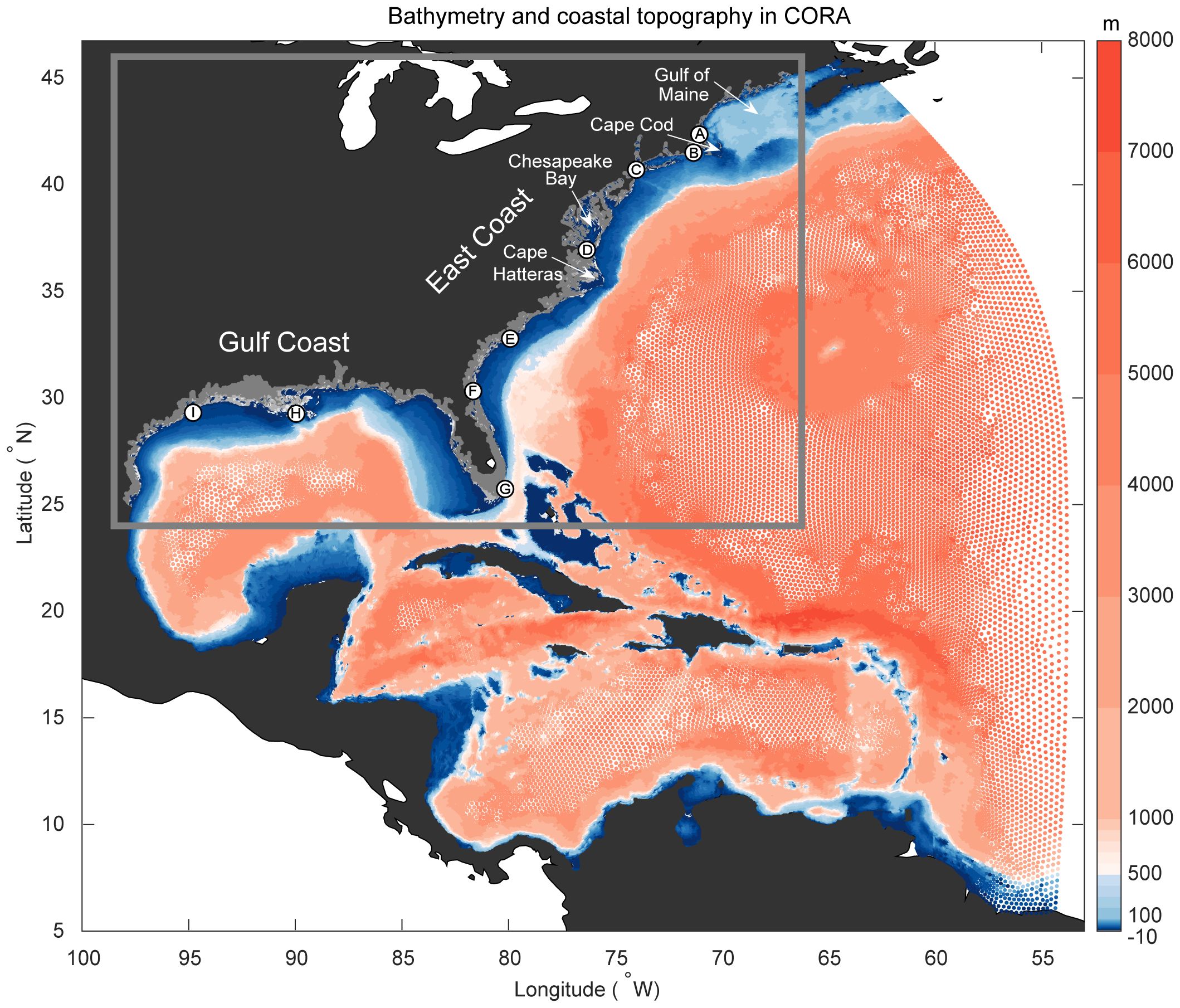
Figure 1 Spatial domain and relative node spacing of the ADCIRC model used for CORA. Bathymetry is indicated at model nodes (color bar; m), with ocean depths to 500 m shaded blue. Inland elevations of the model up to 10 m are shaded gray (negative values). The coastline is indicated by a thin white contour between the blue and gray shadings. A box encloses the focus region of this assessment (Gulf and East Coasts of the U.S. only). Arrows indicate places referred to in the text and letters label locations of focus (referred to later).
While purely barotropic models like ADCIRC have demonstrated effectiveness in resolving tides and meteorologically-driven water level variability (e.g., Bunya et al., 2010; Piecuch et al., 2016), they do not explicitly represent water level responses to baroclinic processes (e.g., variability in major ocean currents such as the Gulf Stream; Calafat et al., 2018; Chi et al., 2018) and seasonal processes such as steric expansion of the water column (e.g., Widlansky et al., 2020). Depending on the use of riverine forcing, they may also be missing these effects (e.g., Piecuch and Wadehra, 2020). Finally, when run for long-term studies such as the current 43-year reanalysis, they would not include processes such as sea level rise, and they would be subject to any slowly varying biases that may occur in the meteorological forcing. To dynamically compensate for these unresolved water level forcings, CORA assimilates coastal water level observations that have been low-pass filtered to remove tidal responses and synoptic events (Asher et al., 2019). Accordingly, CORA is not meant to accurately simulate sea level variability in the offshore North Atlantic where there is no assimilation of water levels and baroclinic processes may dominate.
With recent technological strides in global ocean variability simulations using baroclinic models, the question has arisen of the necessity for the barotropic assimilation framework used in CORA. This question is addressed briefly by comparing CORA to the Copernicus Global 1/12° Oceanic and Sea Ice GLORYS12 Reanalysis (Jean-Michel et al., 2021). Atmospheric forcing fields for GLORYS12 are derived from the same meteorological forcing used in CORA (described in section 2.1); however, data assimilation in the former is focused on satellite-measured sea surface heights and temperatures as well as in-situ measurements of subsurface temperature and salinity profiles. Previously, global ocean reanalyzes using baroclinic models showed poor skill in simulating interannual sea level variability along the East Coast of North America (Piecuch et al., 2016; Long et al., 2021; Widlansky et al., 2023). GLORYS12 possesses a much higher spatial resolution (1/12°) than the reanalyzes previously assessed by those studies, and it seems to well simulate oceanic processes around North America (Amaya et al., 2023; Feng et al., 2024). However, none of the models currently used for global ocean reanalyzes assimilate land-based gauge observations of water levels (sometimes referred to as tide gauge data).
This study assesses the water level characteristics of CORA for the entirety of the U.S. Gulf and East Coasts by comparing reanalysis results with coastal observations from NOAA’s National Water Level Observation Network (NWLON). Focus is on assessing how CORA compares to the water level gauge observations over varying time scales, from the multi-decadal trend to hourly variability. CORA’s results in simulating realistic monthly variability is also compared to the global reanalysis (GLORYS12). Additionally, a case study focused on the Miami, Florida (FL) region is used to demonstrate how CORA can provide a means to quantify coastal inundation. The paper concludes with a discussion of potential opportunities for utilizing this or subsequent versions of CORA to investigate water levels and flooding characteristics along the coast, including in areas lacking long-term water level gauge observations.
The preliminary version of CORA covers the period 1979–2021 at hourly resolution. The ADCIRC model time step was two seconds, and hourly water levels were archived for the full reanalysis by spot-sampling the data at the zero-minute of each hour. The SWAN time step was one hour: at each shared time step, water levels and currents were passed to SWAN and wave radiation stress gradients were passed to ADCIRC. Boundary and tidal potential forcing consisted of the 10 tidal constituents (M2, S2, N2, K2, K1, O1, P1, Q1, Mm, and Mf) from the Oregon State University TPXO 7.2 (Egbert and Erofeeva, 2002), which represent the primary astronomical forcing throughout the region. Atmospheric forcing consisted of 10-m winds and sea level pressure from the European Centre for Medium-Range Weather Forecasts (ECMWF) Reanalysis v5 (ERA5; Hersbach et al., 2020). Model simulation and data storage for CORA was managed by RENCI.
Data assimilation for CORA utilizes coastal observations from the NWLON dataset as described by Asher et al. (2019). This adjustment is accomplished by running the coupled ADCIRC+SWAN without assimilation; calculating daily spatial-difference fields from four-day low-pass filtered modeled and observed water levels using radial basis functions to extrapolate between water level gauges; and, then re-running the coupled ADCIRC+SWAN with an additional mass source and an additional atmospheric pressure component computed using the inverted-barometer equivalent of the difference fields. The data assimilation process, which is described in detail in Asher et al. (2019), is expected to make the coastal water levels in CORA more realistic both around and between observation gauges.
For comparison with NWLON observations, CORA data are extracted using bilinear interpolation of water levels at the three vertices (ADCIRC nodes) of the triangular element encompassing the location closest to the water level gauge. A recursive algorithm is used to check that each node of the selected element always has a water level during the entire reanalysis, otherwise we proceed to check the next closest element to the water level gauge at greater model depths (in one-meter increments). In this manner, we constrain our comparison of observations and CORA to exclusively consider the model nodes that are perpetually submerged, thereby ensuring consistent water level data.
Sea surface height monthly data from the global ocean reanalysis, GLORYS12, were compared to water levels from CORA and observations. For the GLORYS12 gridded dataset, sea levels are extracted from ocean points closest to the water level gauges using the nearest-neighbor method. Since GLORYS12 excluded tidal forcing in the model simulation, the dataset is not used for the assessment of hourly water levels, although there is an opportunity for further studying non-tidal residuals in this reanalysis, if the hourly data is later utilized. Thereby, we compare the performance near the coast of the two reanalysis products (i.e., CORA and GLORYS12) at monthly time scales during their overlapping period (1993–2020).
Our validation of CORA encompassed a total of 105 locations in the NWLON (Table 1). These water level gauges are selected based on data availability and completeness. The selection criteria necessitated at least 10 years of hourly water level data with more than 70% completeness. Among the 105 locations, 52 of them are included in the CORA data assimilation scheme (8 of these assimilated water level gauges are only partially assessed because their records are shorter than 10 years). The water level from CORA is referenced to the Mean Sea Level (MSL). For analyzing hourly data, we first transformed the vertical datums for CORA and observed water levels to the Mean Higher High Water datum (MHHW; i.e., the average height of the highest tide recorded each day at a location). Here, MHHW is calculated during the 2002–2020 epoch for both CORA and observations, using the available recording period therein for the water level gauges. This period of observations is scheduled to become the fifth iteration of the National Tidal Datum Epoch (NTDE5, https://tidesandcurrents.noaa.gov/datum-updates/ntde/).
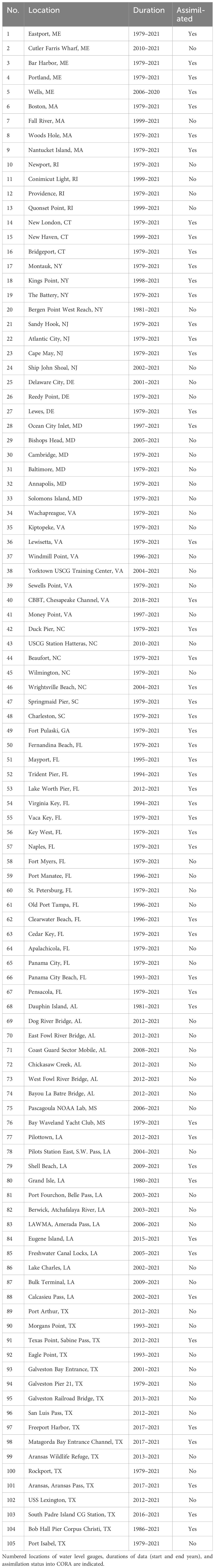
Table 1 Description of observations used in the assessment.
The performance of the two reanalyzes is assessed at various time scales by comparing sea levels from GLORYS12 and water levels from CORA with the water level observations according to the metrics of standard deviation (SD) of each dataset, Pearson correlation coefficient (r), anomaly correlation coefficient (ACC), and root-mean-square error (RMSE). ACC and RMSE are calculated from monthly mean anomalies of reanalyzes and observations. Trends in monthly anomalies as well as the range and peak month of the annual cycle are also compared for the datasets. The annual cycle range represents the difference between the maximum and minimum monthly climatology. The peak month of the mean annual cycle is defined as the month with the highest water level (or sea level) on average. Trends are calculated on the monthly anomalies using least squares linear regressions over a common time period of observations and reanalyzes (nominally 1993–2020); however, the time period is adjusted for water level gauges with shorter records so that the epochs match across datasets (see Table 1). All the metrics are calculated based on the availability of observations, allowing for different time periods in some locations, and omitting some assessments for the water level gauges with very short records (e.g., only four years of observations for CBBT, Chesapeake Channel).
Tide predictions for observations and CORA were made according to calculations of their respective tidal harmonic constituents. We applied the Matlab version of Unified Tidal Analysis and Prediction Functions (UTide) to the detrended hourly water levels during the NTDE5 to obtain up to 68 tidal constituents at each location. These include the principal tidal constituents (including M2, S2, K1, and O1), those associated with long period tides (eg., Sa, Ssa, and Mm), and some non-linear components of the tides. Then, the tide predictions were generated with nodal corrections by using the constituents with power exceeding a minimum signal-to-noise ratio of two, which was nominally 17 and 11 constituents across locations for the observations and CORA, respectively. Lastly, the non-tidal residual was calculated for each location and dataset. We also assessed the performance of CORA in terms of the difference in amplitude and phase of the leading tidal constituent compared to the observations. For the tidal difference assessment, we calculated errors of the respective constituents having the greatest amplitude at each location (indicated in the results), which was usually M2 (principal lunar semidiurnal with a period of 12.42 hours) for the East Coast and either K1 or O1 (lunar diurnal with a period of 23.93 or 25.82 hours, respectively) for the Gulf Coast.
At hourly timescales, CORA is assessed based on its SD, along with calculations of r and RMSE, with respect to the water level observations. Hourly non-tidal residuals used for such calculations were obtained by subtracting the predicted tides from water levels during the entire observational record and reanalysis. CORA’s performance representing the most extreme high-water level events is also assessed according to these metrics. For each location, the 20 highest (and independent) daily maximum water levels were identified in the non-tidal residuals of observations and CORA. Independence of the extreme events is ensured by requiring separation of at least seven days between dates of the highest water levels, otherwise we consider the next highest daily maximum. For these 20 dates of extremes at each location, we extracted five-day windows centered on the peak water levels to compose 100 days of hourly data, and then compared CORA to the observations. These composites include water levels before, during, and after extremely high-water levels, which often exceed established flooding thresholds (section 3.5).
Annual histories of high-water levels for observations and CORA are defined by calculating the respective 2% exceedance thresholds of daily maximum water levels. For this calculation, the trend is either retained or removed in the water levels so that we consider effects of long-term changes and/or higher-frequency variability, respectively. The annual occurrence at a location is the number of days per year that the daily maximum water level exceeds the 2% threshold (calculated during the NTDE5). We compare this statistic between observations and CORA to determine the capability of the reanalysis for describing the 43-year history of high-water levels.
We end the assessment by presenting an example of using CORA to study how coastal flood risk varies in space and time, such as during a severe weather event like a hurricane. This application is shown using a case study of water level and inundation conditions around the cities of Miami and Miami Beach in the southeastern part of FL. For this region, we performed calculations for every model node within a 0.3° latitude × 0.18° longitude (approximately 33 km × 19 km) domain centered on the Virginia Key water level gauge (3277 nodes). We focus especially on conditions during September 2017, which was when Hurricane Irma struck the Florida Keys with Category 4 winds and caused storm-surge flooding in a broad region of the southern East Coast (Juárez et al., 2022).
To assess flood characteristics in CORA, we first categorize model nodes as either having “dry land” or “ocean” characteristics, depending on whether they are dry or wet during every hour of the entire reanalysis. This land/ocean distinction does not include every node, since some places are only sometimes covered by water. Some of these non-ocean nodes are submerged at least once per calendar month and, hence, categorized as “intertidal” zones (i.e., representing places flooded during high tides). It is the remaining nodes, which are not in either of the preceding categories (i.e., dry land, ocean, or intertidal), that we are most interested in for assessing flood characteristics. These so-called “occasionally flooded” nodes have hourly water level data only rarely during the 43-year reanalysis. The “intertidal” region includes wetlands, river floodplains, and partially submerged sandbars, while the “occasionally flooded” nodes may also include other inland places that are only inundated because of extreme events.
For the Miami regional case study, we perform spatial and temporal analysis of all these model-node classifications. Assessing positions of the occasionally flooded nodes reveals where inundation has occurred in CORA. Likewise, considering how the 2% exceedance threshold varies for the ocean nodes may identify spatial differences in the magnitude of water level extremes. We present a flooded-node-hours metric to track temporal changes in the amount of area inundated by water (i.e., the number of flooded-nodes per hour summed over the region of interest, and then binned by month). The resulting time series provides a description of how inundation is simulated in the occasionally flooded zone of CORA for not only the area immediately around the Virginia Key water level gauge, but also the Greater Miami region vulnerable to high tides, storm surges, as well as sea level rise and variability.
We assess the long-term trends of water levels in CORA at assimilated and non-assimilated NWLON locations (Table 1), as well as make comparisons with sea level trends in GLORYS12, thereby determining abilities of both reanalyzes to replicate observed changes at decadal time scales. Coastal water level trends are associated with a variety of oceanic and geological processes that are measured and resolved in various capacities by these datasets. Specifically, GLORYS12 is designed to better simulate open ocean and global mean sea level changes, rather than relative coastal water level changes, which may have contributions due to land subsidence or uplift. Relative water level changes are measured by coastal gauges and, therefore, these effects are included in the assimilation algorithm used to compute CORA. However, land subsidence can be a highly localized process (e.g., Buzzanga et al., 2020, Buzzanga et al., 2023; Ohenhen et al., 2023). Hence, relative water level changes assimilated into CORA may not always be representative of subsidence or uplift away from water level gauges, even over relatively short distances.
Figure 2 shows the linear trend of monthly anomalies from all the water level gauges, and the difference in trend for the reanalyzes at nearby locations. The sea level trend bias in GLORYS12 is homogeneously negative near the Gulf and East Coast locations that we assessed (Figure 2B; see also Supplementary Table 1), because GLORYS12 simulates oceanic processes and does not capture information about differences in relative sea-level rise observed by the water level gauges (Figure 2A). The trend for GLORYS12 averaged over all locations is less than half the observed trend of 8.95 mm yr-1 (i.e., a bias of nearly -6 mm yr-1). These trend rates equate to sea level rise from 1993–2020 of 0.294 m for observations and only 0.084 m for GLORYS12. GLORYS12 trends are biased low near all the water level gauges considered, partly because glacial isostatic adjustment (GIA) causes land subsidence of the East Coast south of Massachusetts (Harvey et al., 2021). The differences compared to water level gauges are especially large for the western Gulf Coast, where anthropogenic extraction of subterranean fluids caused localized subsidence and faster sea level rise (e.g., 14.07 mm yr-1 observed versus 3.74 mm yr-1 in GLORYS12 at Eagle Point, TX; Supplementary Table 1). The slower sea level rise in GLORYS12 for the western Gulf Coast is partly explained by the fact that the reanalysis does not resolve changes in land elevations, which are subsiding around many of the water level gauges there (Kolker et al., 2011; Harvey et al., 2021). Trends on the East Coast in GLORYS12 more closely resemble the observations (respectively, 3.46 mm yr-1 versus 5.71 mm yr-1 at Charleston, SC; Supplementary Table 1). However, there is still considerable bias on the East Coast, especially between Cape Hatteras and Cape Cod where the regional average trend in GLORYS12 is about 3 mm yr-1 less than observed (Figure 2B). Along the Mid-Atlantic Coast, the GIA trends unresolved by GLORYS12 can be as large as 2 mm yr-1 (Harvey et al., 2021). Besides unresolved processes in GLORYS12, its resolution (1/12°) could explain some disparities in the trends for estuaries like the Chesapeake Bay area where water level gauges are far removed from the nearest-ocean model grid point (Feng et al., 2024).

Figure 2 (A) Long-term linear trend of monthly anomalies (mm yr-1). Difference in trend with respect to (A) observations for (B) GLORYS12 nearest to the water level gauges and (C, D) CORA nearest to the water level gauges that are either assimilated or not assimilated, respectively, as listed in Table 1. Solid circles represent trends calculated between 1993–2020, dotted circles represent locations where availability of the observations differs from that complete epoch necessitating a shorter period to be used for the trend calculation (at least 10 years), and dotted triangles represent assimilated locations with even shorter water level gauge records (only shown for the trend analysis). Six locations have trends exceeding the color bar range (above 20 mm yr-1); four of which have records shorter than 9 years.
CORA produces water level trends that resemble observations, both around the assimilated and non-assimilated gauges (Figures 2C, D). For CORA, the average trend of all locations is only 0.66 mm yr-1 less than the observed trend (8.95 mm yr-1). The overall better agreement in the average trend is likely due to the ability of CORA assimilation to approximate the smoothly varying GIA field over the domain. Near the assimilated water level gauges, CORA trends are even more aligned with observations (on average, only 0.44 mm yr-1 less than the observed trend of 8.37 mm yr-1). Around the non-assimilated water level gauges, in contrast, trend differences between CORA and observations are slightly larger (-0.88 mm yr-1 on average). The most substantial trend differences in CORA are for parts of the western Gulf Coast around water level gauges that were not assimilated (e.g., 7.79 mm yr-1 less than the 14.07 mm yr-1 observed at Eagle Point, Galveston Bay, TX), which is presumably due to the smaller spatial scales of the non-GIA subsidence processes dominant in this region. In the Chesapeake Bay, where only two water level gauges were assimilated (Lewisetta, VA and CBBT, Chesapeake Channel, VA; Table 1), the similarity between trends in observations (Figure 2A) and CORA (Figures 2C, D) highlights an advantage of non-localized assimilation (i.e., trends resemble observations even away from the assimilated water level gauges; Asher et al., 2019).
In general, CORA describes well the observed trends for the Gulf and East Coasts, including around both assimilated and non-assimilated water level gauges (Figures 2C, D). However, there are a few places on the coast where the water level trend in CORA needs further scrutiny, especially where there are relatively large distances between assimilated water level gauges or complexities in the coastal bathymetry and shoreline geometry (e.g., channel constrictions, multiple inlets) requiring finer model resolution to resolve (e.g., tidal dynamics in lagoons; Bilskie et al., 2019). Supplementary Figure 1 compares the water level trends for CORA and observations along the coast at three spatial scales (full domain, regional, and local), using southern FL as an example of the latter two areas. There is evidence that the regional coastline shape and distance between water level gauges affects the trend in CORA. An example of this concern is between Lake Worth and Trident Pier (Cape Canaveral) on the eastern coast of FL (Supplementary Figure 1) where there is a pronounced along-shore gradient of the water level trends in CORA, despite the water level gauges at the southern and northern bounds of this region being used in the assimilation and having comparable trends (Supplementary Table 1). A further challenge in the CORA assimilation arises when the observation periods differ across nearby water level gauges such as between the Virginia Key and Lake Worth locations shown in Supplementary Figure 1 (record durations are listed in Table 1). We consider locally varying water level trends in CORA again when describing applications (section 3.6).
To begin assessing the proficiency of the reanalyzes in capturing seasonal variability, we examine the mean annual cycle characteristics. The focus is first on the timing of the annual cycle, as indicated by the peak month at water level gauges, as well as for sea levels from GLORYS12 and water levels from CORA (Figures 3A–D; Supplementary Figure 2 shows the annual cycle across all months). The annual cycle typically peaks during September or October at most of the water level gauges on the Gulf and East Coasts (Figure 3A). These months are when ocean temperatures are usually the warmest (i.e., during late summer or early fall), which is associated with thermal expansion of seawater and therefore higher sea levels for the open ocean and water levels at the coast (see also Figure 2 in Widlansky et al., 2020). Other factors driving the observed coastal water level annual cycle include Gulf Stream dynamics (e.g., around Virginia Key, FL; Ezer and Dangendorf, 2022) and riverine outflows (e.g., around the Gulf of Maine, which has an earlier peak of the annual cycle because of remote effects from the St. Lawrence River; Piecuch and Wadehra, 2020).
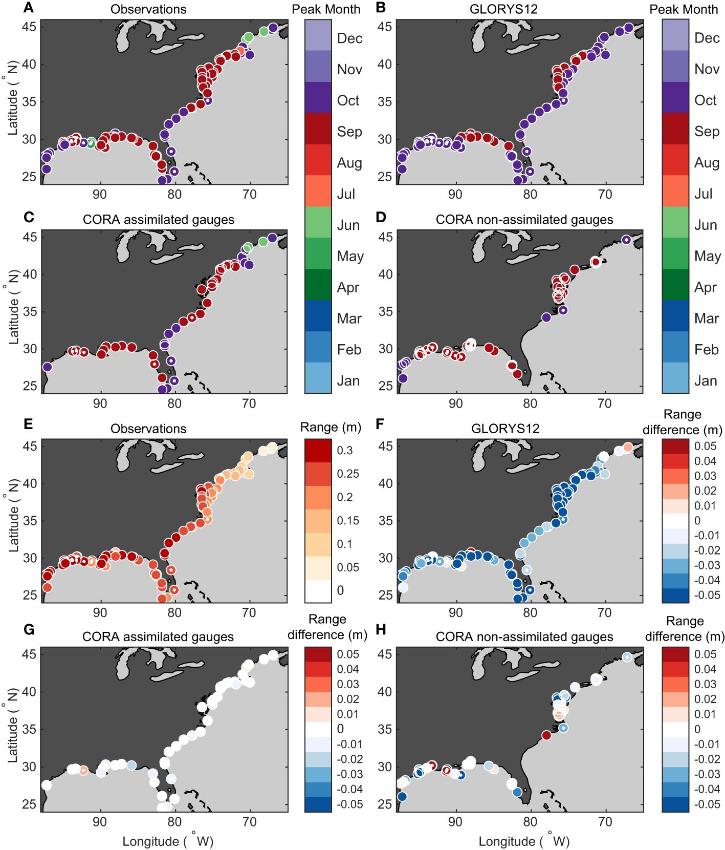
Figure 3 Annual cycle characteristics. Top: The peak month of the annual cycle for (A) observations, (B) GLORYS12 nearest to the water level gauges, (C) CORA at assimilated water level gauges, and (D) CORA at non-assimilated water level gauges. Epoch criteria for the solid and dotted circles are explained in the Figure 2 caption. Bottom: The range of the annual cycle (m) is calculated from the monthly climatology for (E) observations. The difference in range of the annual cycle (m) with respect to water level gauges, for (F) GLORYS12, (G) CORA at assimilated water level gauges, and (H) CORA at non-assimilated water level gauges.
Both GLORYS12 and CORA resolve the timing of the annual cycle peak to within a month at most locations (Figures 3B–D). GLORYS12, using a baroclinic ocean model, directly simulates thermal expansion and Gulf Stream dynamics (Amaya et al., 2023). For the Southeast Coast, the annual peak timing of high sea levels in GLORYS12 is very similar to the water level gauges (e.g., during October at Charleston, SC). Likewise, there is close agreement of the annual cycle peak months between GLORYS12 and the water level gauges for most locations on the Mid-Atlantic, Northeast, and Gulf Coasts. Around the Gulf of Maine, however, there are discrepancies of a couple of months (e.g., at Portland, ME), which is possibly related to the absence of riverine forcing in GLORYS12 (Jean-Michel et al., 2021). CORA has even better agreement with the observed annual cycle peak timing, both at the assimilated and non-assimilated water level gauges (Figures 3C, D). The apparent accuracy of CORA is due to the assimilation of water level observations because there is no thermal expansion in the ADCIRC barotropic model, nor is riverine outflow directly included in the reanalysis. Around non-assimilated water level gauges in CORA (Figure 3D), the similarity of the annual cycle peak month to observations suggests that the assimilation procedure correctly adjusts the timing of the water level climatology at these locations as well.
Amplitude of the annual cycle is indicated by the range between the maximum and minimum values of the monthly mean annual cycle (Figures 3E–H). According to the water level gauges (Figure 3E), the annual cycle is larger in magnitude for the Gulf and Southeast Coasts (e.g., 0.275 m at Charleston, SC) compared to locations north of Cape Hatteras (e.g., 0.209 m at Ocean City Inlet, MD). There are exceptions to these general observations for the Mid-Atlantic Coast, such as the locally larger annual cycles in some estuaries, including Chesapeake Bay (e.g., 0.285 m at Baltimore, MD), compared to nearby water level gauges closer to the open ocean (e.g., 0.219 m at Kiptopeke, VA). The smallest annual cycle magnitudes are observed north of Cape Cod (e.g., 0.076 m at Portland, ME) where there is limited oceanic thermal expansion during the summer (Widlansky et al., 2020).
The annual cycle amplitudes in GLORYS12 and CORA resemble the water level observations almost everywhere (Figures 3E–H), although some notable differences exist. Averaging the annual cycle ranges for the locations shown in Figure 3, there are only slight differences between the observations (0.239 m) and CORA, which is 0.025 m less at the assimilated water level gauges and only 0.006 m more at the non-assimilated locations. For GLORYS12, there is a larger difference of the average annual cycle range (0.054 m less than observed). Regionally, the Mid-Atlantic Coast stands out as an area of discrepancy in the annual cycle range between observations and GLORYS12 (e.g., 0.254 m versus 0.156 m, respectively, at Windmill Point, VA). For CORA, the annual cycle range is much closer to observations around all the assimilated water level gauges (Figure 3G) as well as most of the non-assimilated locations (Figure 3H), such as around the Chesapeake Bay (e.g., 0.248 m at Windmill Point, VA). There are much larger discrepancies in the CORA annual cycle around a few of the other non-assimilated water level gauge locations, like at Wilmington, NC on the Cape Fear River where the reanalysis range is 0.068 m more than observed (Figure 3H).
Monthly anomalies are computed for observations, GLORYS12, and CORA for each water level gauge location on the Gulf and East Coasts by removing the mean annual cycle and linear trend from the data. To quantitatively assess the monthly variability, we employed statistical metrics including the SD, ACC, and RMSE (see Section 2.2). Results of the monthly variability assessment are depicted in Figure 4 and listed in Supplementary Table 2. Time series of the monthly anomalies are also shown for selected locations in Figure 5.
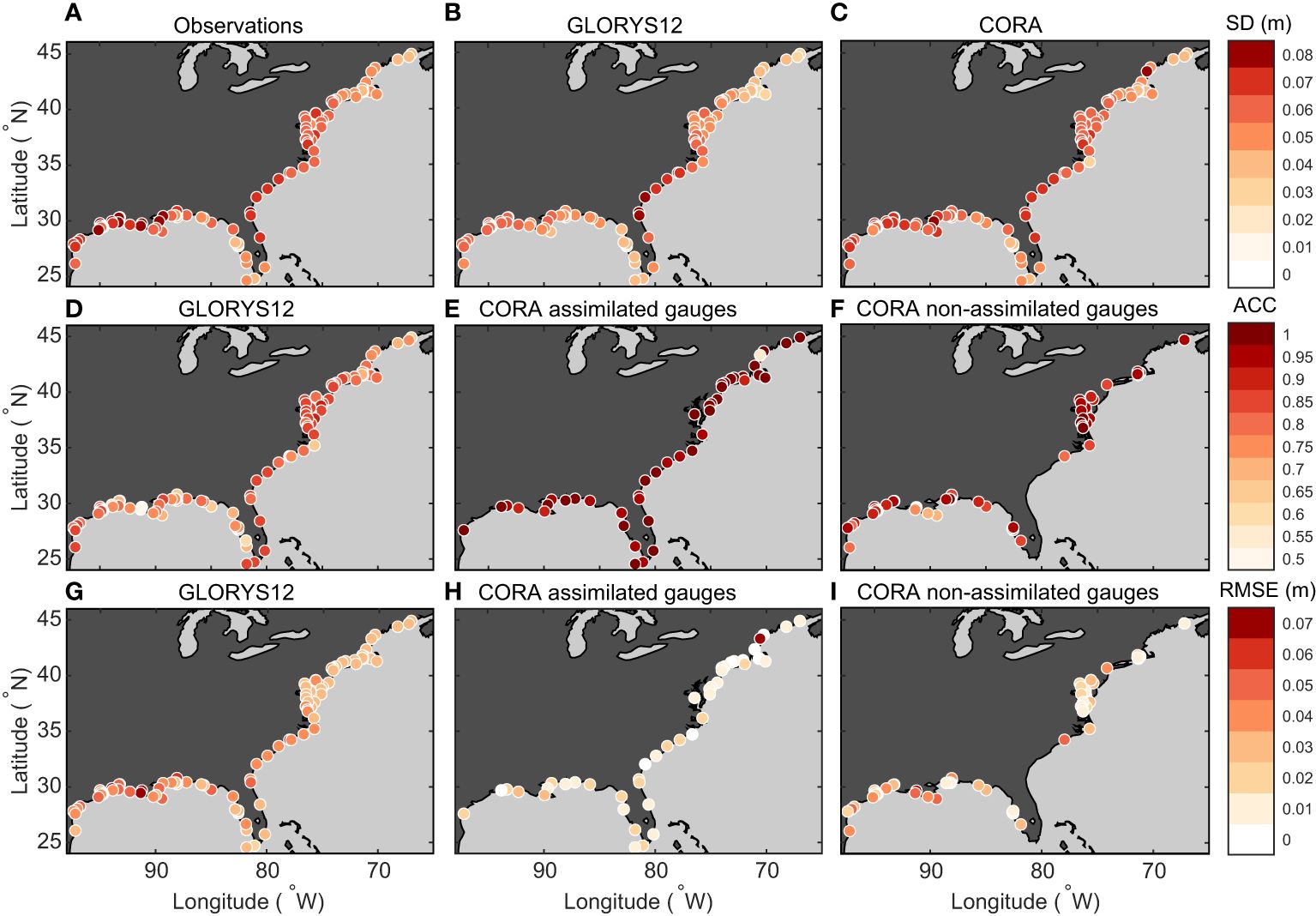
Figure 4 Comparison of monthly anomalies between observations and reanalyses. The SD (m) for (A) observations, and nearest to the water level gauges for (B) GLORYS12 and (C) CORA. The ACC between monthly mean anomalies from observations and (D) GLORYS12 nearest to the water level gauges, (E) CORA at assimilated water level gauges, and (F) CORA at non-assimilated water level gauges. The RMSE (m) of monthly mean anomalies from observations compared to (G) GLORYS12 nearest to the water level gauges, (H) CORA at assimilated water level gauges, and (I) CORA at non-assimilated water level gauges. Varying time periods are used for different locations, depending on availability of the observations (Table 1), while maintaining consistent time periods for each location across metrics (A–I).
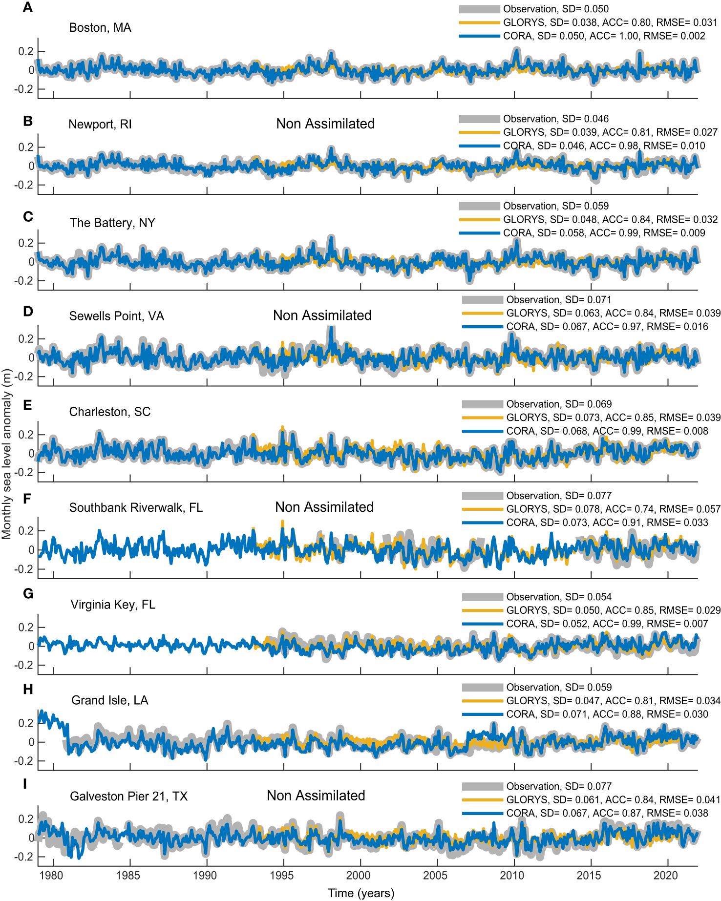
Figure 5 Monthly anomalies (m) for observations (gray; when available), and nearest to the water level gauges for GLORYS12 (yellow; 1993–2020) and CORA (blue; 1979–2021). The locations are (A) Boston, (B) Newport, (C) The Battery, (D) Sewells Point, (E) Charleston, (F) Southbank Riverwalk, (G) Virginia Key, (H) Grand Isle, and (I) Galveston Pier 21. Water level gauges not assimilated in CORA are indicated. The legend displays the ACC and RMSE of GLORYS12 and CORA compared to observations as well as the SD values for each.
For most of the water level gauges on the Gulf and East Coasts, the amount of monthly variability in both GLORYS12 and CORA aligns closely with observations (i.e., SD values are comparable, as seen in Figures 4A–C and Supplementary Table 2). Results for the Charleston, SC water level gauge are an example of realistic amounts of monthly variability in the reanalyzes compared to observations (i.e., the SD values are identical for CORA and only 0.004 m larger for GLORYS12; Figure 5E). Interestingly, monthly variability at locations near Charleston on the Southeast Coast is typically larger in GLORYS12 compared to the observations as well as CORA (Figures 4A–C; values are listed in Supplementary Table 2). Averaged over all the locations from Texas to Maine, monthly variability in CORA is somewhat less than the observations (SD values of 0.058 m versus 0.063 m). Around the assimilated water level gauges, there is no apparent difference in CORA compared to observations as far as the amount of monthly variability (i.e., the average bias of the SD values is negligible).
The ACC metric reveals clear distinctions in performance of GLORYS12 and CORA when compared to observations (Figures 4D–F). GLORYS12 has a weaker correlation with observations overall (Figure 4D), both for the Gulf Coast (e.g., the ACC is 0.81 at Grand Isle, LA; Figure 5H) and the East Coast (e.g., ACC is 0.85 at Charleston, SC; Figure 5E). CORA is much more strongly correlated with the observed monthly variability, both overall (Figures 4E, F) and for these examples (ACC values of 0.88 and 0.99, respectively; see Figure 5 for time series at these and other locations). CORA performs similarly well according to this correlation metric for most other locations on the East Coast, regardless of assimilation status of the nearby water level gauges (e.g., at the non-assimilated Sewells Point, VA location, the ACC is 0.97; Figure 5D). Performance as measured by ACC is relatively low along the Gulf Coast (e.g., 0.88 at the Grand Isle assimilated water level gauge; Figure 5H). Considering the time series comparisons with the Grand Isle gauge (Figure 5H), it is unknown why there is a noticeable offset in CORA during 2007–2010 compared to both the observations and GLORYS12. Such offsets from observations of monthly anomalies are rare in CORA, even among locations around the non-assimilated water level gauges (e.g., as shown in panels B, D, F, and I of Figure 5).
The RMSE metric for GLORYS12 and CORA compared to the observations indicates mostly similar performances of the reanalyzes overall (Figures 4G–I), although the values for GLORYS12 are slightly higher everywhere compared to CORA (Supplementary Table 2). Whereas Cape Hatteras marks a clear distinction in the amount of RMSE for GLORYS12 (Figure 4G), no such spatial demarcation is evident in CORA (Figures 4H, I). GLORYS12 exhibits larger errors along the Southeast and Gulf Coasts, where monthly variability also is larger (see SD values in Figure 4A). Overall, the RMSE of CORA for monthly variability is very small in absolute terms (e.g., 0.008 m at Charleston, SC compared to that assimilated water level gauge) and relative to GLORYS12, which has five times larger error for this example location (Figure 5E). For CORA, there are only six locations between Texas and Maine where both the ACC is below 0.80 and the RMSE exceeds 0.04 m (e.g., Wilmington, NC; Supplementary Table 2), which is a substantial improvement compared to GLORYS12 (25 such locations).
The fidelity of CORA in resolving tides is evaluated through its capability to describe tidal constituents that match the observed characteristics. We specifically focus on the leading constituent at each location as described in Section 2.2 (i.e., typically the M2 principal lunar semidiurnal tide for the East Coast and either the K1 or O1 lunar diurnal tide for the Gulf Coast). These tidal constituents are calculated from hourly water levels, and differences between CORA and observations are depicted in Figure 6.
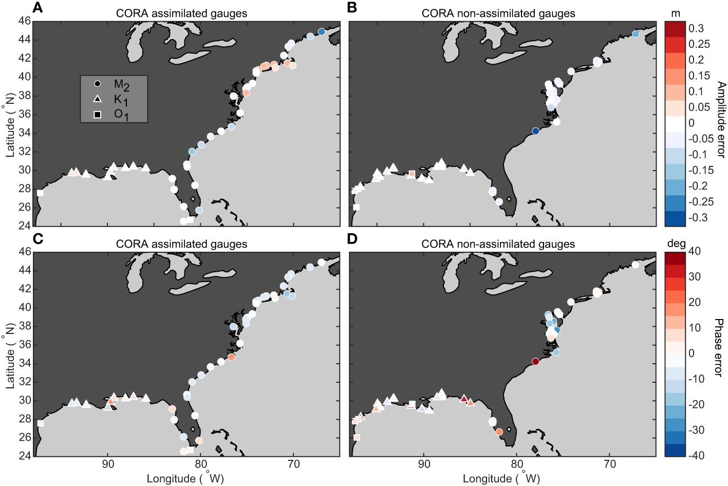
Figure 6 Errors in the leading tidal constituent in CORA compared to observations. (A, B) The amplitude errors (m) for assimilated and non-assimilated water level gauge locations, respectively. (C, D) The phase errors (deg) for similar location distinctions. The leading constituents are indicated by circles (M2), triangles (K1), and squares (O1).
This assessment reveals mostly minor biases in the amplitude of the leading tidal constituents. Biases are slightly negative overall, and larger on average for the East Coast (-0.034 m) compared to the Gulf Coast (-0.013 m). Regionally, however, biases are mostly positive between Cape Hatteras and Cape Cod, especially around assimilated water level gauge locations (Figure 6A). Due to the low-pass filtering method of the data assimilation, we did not expect assimilation status to explain a large difference in performance resolving tides (i.e., comparing Figures 6A, B). Notably, two non-assimilated locations on the East Coast display underestimations of the lunar semidiurnal tide, with M2 amplitude errors exceeding -0.20 m (Wilmington, NC and Cutler Farris Wharf, ME; Figure 6B). The Wilmington water level gauge is located on the Cape Fear River approximately 30 km from its mouth at the Atlantic Ocean, and Cutler Farris Wharf is located near the Bay of Fundy where tides exceed 10 m. Although CORA has limitations depicting tides in such specific locations, tidal amplitudes in the reanalysis are mostly similar to observations.
In terms of tidal phase biases, CORA compares well with observations at most locations (Figures 6C, D). The average M2 tidal phase bias for the East Coast is about -4 degrees, which is equivalent to an approximately 8-minute offset for this constituent. Small negative phase biases suggest that there are many locations on the East Coast where the M2 tide in CORA leads the observations by a few minutes. However, there are clearly exceptions where much larger (and positive) biases exist for the M2 constituent, such as at Wilmington, NC (37 degrees or 76 minutes of lag). The lagging tide at Wilmington in CORA is most likely due to insufficient resolution of the Cape Fear River in the HSOFS mesh but may also be affected by the absence of river influx in the model. For the Gulf Coast, average K1 or O1 tidal phase biases are also positive but rather small (5 degrees or about 20 minutes of lag), although the span of biases near non-assimilated water level gauges is substantial (-12 degrees to +35 degrees or 49 minutes lead to 143 minutes lag on average among these tidal constituents). Explaining the causes of these tidal errors in CORA requires further study, which we briefly discuss in Section 4.
Non-tidal water levels for each dataset are calculated by subtracting the predicted tides from the observations and CORA, respectively. Using the non-tidal residuals, which do not include long-term trends, we assess the capability of CORA to accurately simulate hourly variability. The evaluation method of comparing with the observations and applying performance metrics is like what was used in the monthly variability assessment (Section 3.3). Figure 7 illustrates the results for evaluating the hourly non-tidal residuals of CORA according to the amount of variability (SD), correlation with observations (here using the Pearson’s correlation coefficient, r, instead of ACC), and error magnitude (RMSE).
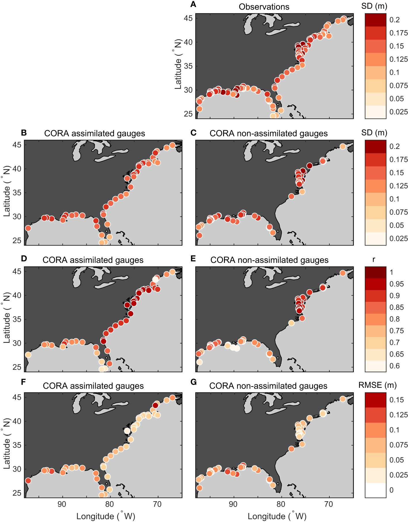
Figure 7 Comparison of hourly non-tidal residuals between observations and CORA. (A–C) The standard deviation (SD in m) for observations, CORA at assimilated water level gauges, and CORA at non-assimilated water level gauges, respectively. (D, E) The Pearson correlation coefficient (r) with respect to observations for CORA at assimilated and non-assimilated water level gauges, respectively. (F, G) The RMSE (m) with respect to observations for CORA at assimilated and non-assimilated water level gauges, respectively. The r and RMSE values at one non-assimilated water level gauge are outside of the color bar ranges (0.28 and 0.334 m at Berwick, Atchafalaya River; see Supplementary Table 2).
The amount of hourly non-tidal variability, as indicated by the SD values in Figure 7A for the observations (0.159 m on average), is much greater than monthly variability (Figure 4A; 0.063 m). Along the Gulf and East Coasts, SD values of the hourly observations range from 0.207 m (Eagle Point, Galveston Bay, LA) to 0.123 m (Cutler Farris Wharf, ME). Hourly variability in CORA is comparable in magnitude to the observations at most of the assimilated and non-assimilated locations (Figures 7B, C; see also Supplementary Table 2). However, there are isolated examples of large biases in non-tidal variability, such as at Pilots Station East, LA where the SD is much smaller in CORA (0.139 m) compared to the water level gauge (0.212 m).
Correlations are strong between the hourly non-tidal water levels in observations and CORA (Figures 7D, C). Overall, 20 out of 44 assimilated water level gauges have an r value exceeding 0.9 (Supplementary Table 2). For the comparison with non-assimilated gauges, r values are similarly strong at roughly a quarter of the locations (14 out of 53). For both the assimilated and non-assimilated water level gauges, r values are higher on average for the East Coast (0.89 and 0.90, respectively) compared to the Gulf Coast (0.79 and 0.76). There are exceptions of much weaker correlations at some locations, however, such as at Berwick, LA, which is located on the Atchafalaya River away from the Gulf Coast (the r value there is only 0.28, and CORA also has a much lower SD than observed; Supplementary Table 2). There are other locations on the Gulf Coast with relatively weak r values (e.g., 0.67 at the Key West, FL assimilated water level gauge). Much stronger correlations exist nearly everywhere on the East Coast, including around non-assimilated locations (e.g., 0.95 at Solomons Island, MD, which is on the Patuxent River near the Chesapeake Bay).
Assessment of the RMSE values offers additional insights into the efficacy of CORA for describing the hourly variability of non-tidal water levels (Figures 7F, G). For the East Coast, RMSE values are low compared to the SD values (Figures 7A–C), especially at the assimilated water level gauges (the average error is only 0.065 m at these locations). For the Gulf Coast, RMSE values are somewhat higher, although still much less than the local SD values (average errors of 0.095 m and 0.103 m, respectively, at assimilated and non-assimilated locations). Performance of CORA around Berwick, LA is again an exception according to the RMSE metric (0.334 m). Other than that non-assimilated water level gauge, we see no systematic differences in the RMSE metric for the hourly variability based on assimilation status.
Figure 8 shows the assessment of hourly variability during high-water level extreme events. We identified the 20 highest (independent) water levels in the data and evaluated the hourly non-tidal residuals within a five-day window centered around each event (i.e., assessing 100-day composites). This extreme event criteria selects water levels that exceed NOAA-defined thresholds for minor flooding occurrence (Sweet et al., 2018) at most locations (e.g., Supplementary Figure 3). There is larger variability in these composites of high-water level events compared to assessing the entire 43-year time series, for both observations and CORA (SD values of 0.302 and 0.293, respectively; Figures 8A–C). During the high-water level events, there are only subtle differences in SD values between locations around assimilated and non-assimilated water level gauges in CORA (0.312 and 0.277, respectively), with observed variability being slightly higher for these subsets (0.317 and 0.291). Correlations are strong between CORA and observations during times of high-water level extremes (r values exceed 0.9 at 66 out of 97 locations; Figures 8D, E). Likewise, the majority of RMSE values are below 0.15 m (81 out of 97; Figures 8F, G). Only a few notable exceptions of locations with poorer performance exist in CORA, such as at Wilmington, NC (r and RMSE values of 0.64 and 0.316 m). At most other locations, CORA performs well during the high-water level events according to these metrics of correlation and error, including around non-assimilated water level gauges (e.g., 0.97 and 0.081 m at Newport, RI).
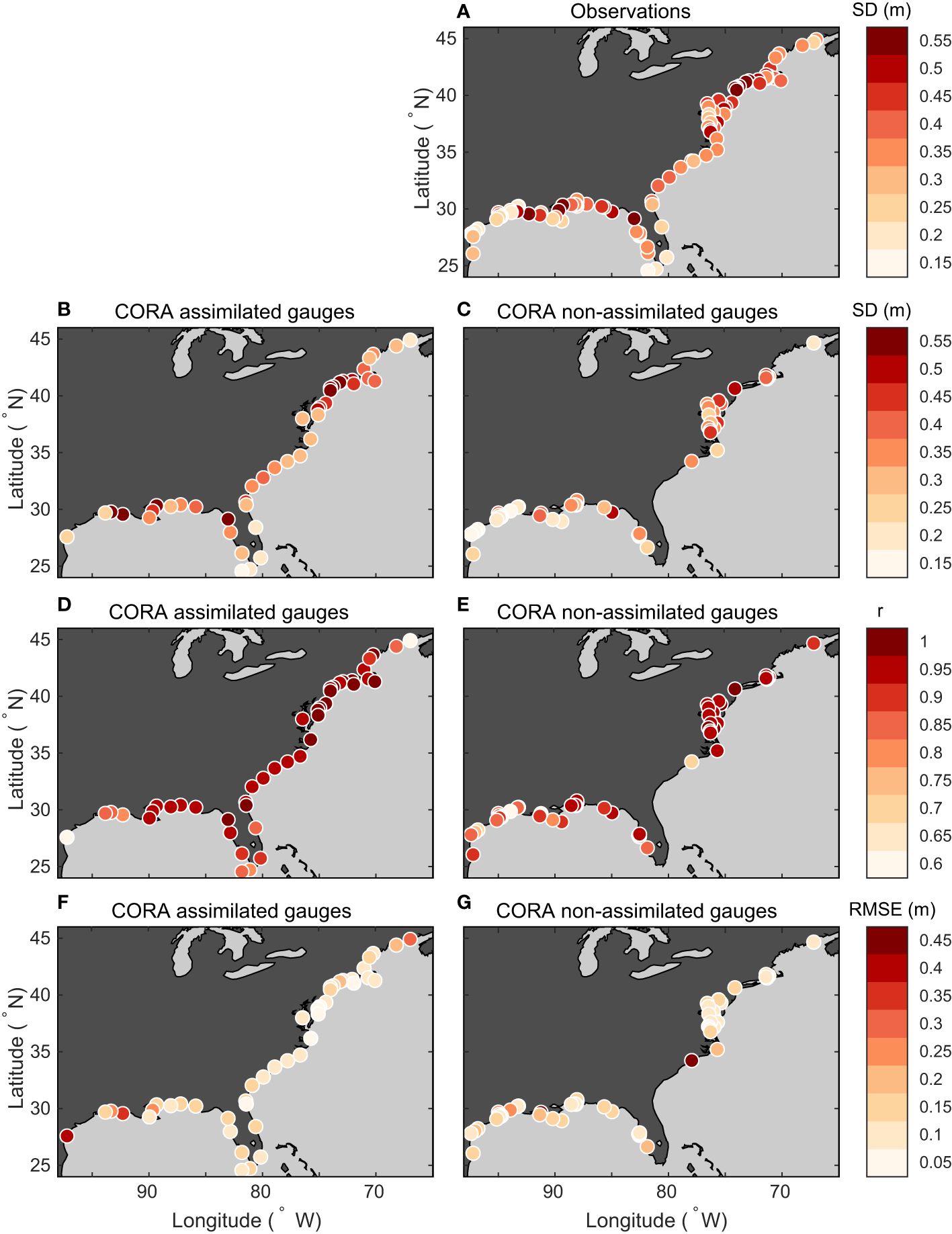
Figure 8 Similar to Figure 7, except for comparing hourly non-tidal residuals during 100-day composites containing the 20 highest water levels observed at each location.
To further elucidate CORA’s performance, we consider nine time series corresponding to locations previously assessed for monthly variability (Figure 5) but now for hourly water levels (Figure 9). We use September 2017 as an example of the tidal and non-tidal variability observed on the Gulf and East Coasts. The observed tidal cycles are mostly well captured by CORA, as seen by the close correspondence between the water levels overall (left column of Figure 9; especially panels A–E, which are for the East Coast locations). Whereas for the Gulf Coast locations (Figures 9H, I), there appears to be more deviation between observations and CORA. Some of the discrepancies in hourly water levels may be attributed to non-tidal diurnal oscillations that CORA and its ERA5 forcing potentially fail to capture (e.g., coastal sea breezes). These discrepancies could also result from other spurious characteristics of the model configuration. Another location of substantial bias in tidal amplitude is Southbank Riverwalk, FL (Figure 9F; this non-assimilated location was not considered in previous assessments because its data record is only from 2015–2021), which is on the St. Johns River about 30 km upstream from the Atlantic Ocean and where meteorological forcing has a dominant influence on water levels (Bacopoulos et al., 2009).
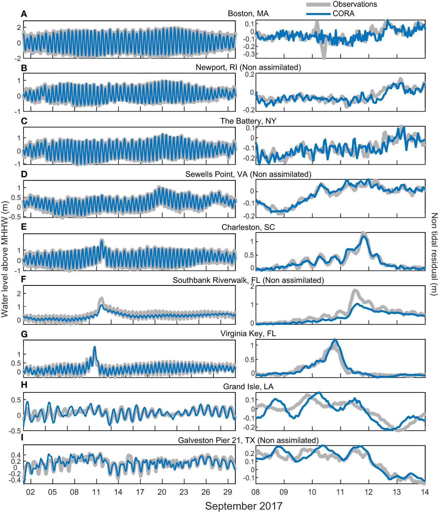
Figure 9 Hourly time series of water levels and non-tidal residuals (m) for observations and CORA. Gray lines represent water level gauges and blue lines represent CORA for the same locations as in Figure 5. Water levels with respect to the MHHW datums are shown for September 2017 (left panels), and the non-tidal residuals are shown for six days around when Hurricane Irma made landfall in FL on September 10, 2017 (right panels).
We choose six days around when Hurricane Irma struck the Florida Keys on September 10, 2017 to show the hourly non-tidal residuals (Figure 9; right column). Hurricane Irma’s storm surge was directly associated with over a meter of water level rise observed that day at Virginia Key, FL, which is in Biscayne Bay near Miami. The non-tidal residual exceeded 1 m above MHHW at the water level gauge, despite being about 180 km from where Hurricane Irma made landfall. Large storm surges were observed along much of the Southeast Coast, such as the record-high-water level at Southbank Riverwalk on the St. Johns River (1.7 m; Figure 9F). There was a substantial water level rise in CORA at that non-assimilated location (1.01 m). The next day at Charleston, SC, a similarly high non-tidal residual was observed and well depicted by CORA (Figure 9E). Water levels exceeded tide predictions much farther north on the East Coast as well, although only by around 0.10 m (e.g., at Sewells Point, VA; The Battery, NY; Newport, RI; and, Boston, MA as shown in Figure 9). CORA effectively described the timings of non-tidal residuals observed by all six water level gauges on the East Coast. Magnitudes were mostly realistic in CORA, however there was a clear low bias at the Southbank Riverwalk. Another example when CORA performed particularly well depicting observed storm surges was during Hurricane Sandy in 2012, regardless of assimilation status of the nearest water level gauge (e.g., approximately matching the 1.5 m non-tidal residual observed at Newport, RI; Supplementary Figure 4). We found that CORA performed similarly well resolving water levels for many other large storms, at least at locations away from the core of most intense winds as experienced in hurricane eye walls.
CORA is designed to serve applications in assessing the frequency and severity of coastal flooding associated with high-water levels. Potential applications include conducting regional frequency analyses of water level characteristics, assessing shifts in the mean conditions (e.g., of tidal datums such as MSL and MHHW), and understanding the spatial extent of flooding due to very high tides and storm surges combined with sea level rise and variability. Most importantly, CORA provides the capability to evaluate changing flood risks both near and away from existing water level gauges. We briefly demonstrate several such applications using this preliminary version of CORA, which performs well in describing the observed water level characteristics for the Gulf and East Coasts (Sections 3.1–3.5).
Figure 10 illustrates the annual number of daily maximum water levels above the 2% exceedance threshold according to the observations and CORA, which respectively average 0.434 m and 0.422 m above MHHW for the 2002–2020 epoch (Supplementary Table 1 lists the thresholds for each location and Supplementary Figure 3 shows the distribution of water levels in relation to the thresholds for example locations). During the recent decade, there has been a clear increase in days experiencing such extreme water levels according to observations (Figure 10A), which has been widely reported (e.g., Sweet and Park, 2014; Wahl et al., 2015). CORA captures this overall increase in occurrence of extremely high-water levels (Figure 10B). There is a close correspondence between observed characteristics and CORA at most of the locations assessed (e.g., at Virginia Key during 2017, 10 and 8 days, respectively). The increase for the Gulf Coast is particularly evident in both the observations and CORA, especially since 2015 (Figure 10C). Water level extremes likewise became more frequent during this time for the East Coast, with the top five years of most occurrences all since 2017 (Figure 10C).
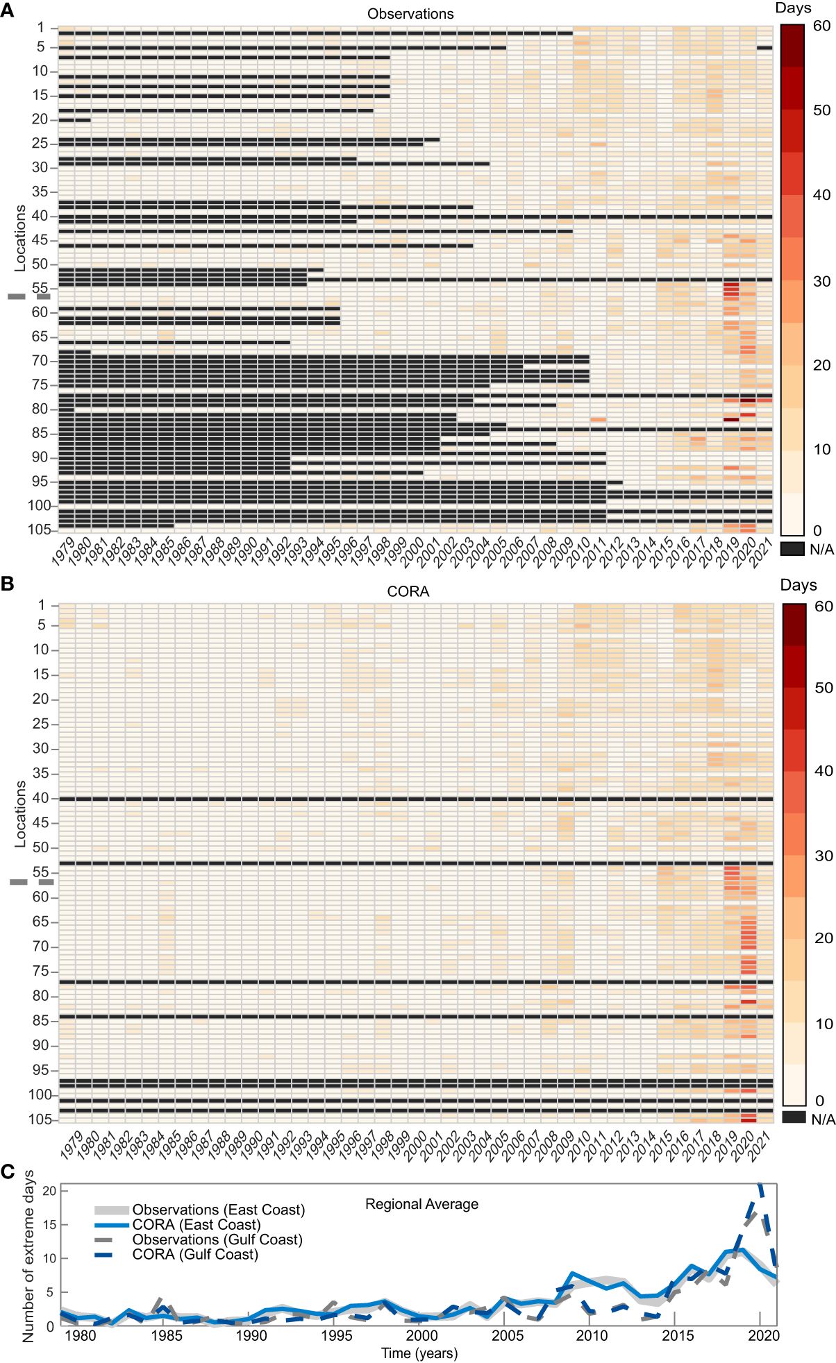
Figure 10 Annual occurrence of extreme water levels according to the 2% exceedance threshold with respect to MHHW for locations on the Gulf and East Coasts. (A) Results from observations (years with unavailable data for a location are gray). (B) Results from CORA (locations not assessed for 2% exceedance are gray; Supplementary Table 1). Color shading indicates the number of days per year when the maximum water level is above the 2% exceedance threshold at a particular location. Numbers on the y-axes indicate every fifth location (see Table 1 for the water level gauge names). Locations are organized by latitude and region, with the northernmost (East Coast) at the top and a dashed line separating the Gulf Coast at the bottom. (C) Regionally averaged annual occurrence of extreme water level days: Solid (dashed) lines are for the East (Gulf) Coast and gray (blue) colors are for the observations (CORA).
Most of the increased occurrence of extremely high-water levels during the 43-year reanalysis, and especially since 2015, is explained by sea level rise (Figure 10). Considering the detrended hourly water levels, there is no overall increase in the annual occurrence of high extremes (Supplementary Figure 5). However, correspondence between individual years remains in the detrended data, such as the large number of high-water levels during 2020 previously noted at the Gulf Coast water level gauges and associated CORA locations.
Tidal datums also changed because of sea level rise, with MSL and MHHW during the 2002–2020 epoch higher everywhere compared to during 1983–2001, which is the prior NTDE (see Supplementary Table 1; and, noting that observations are unavailable at some locations for the earlier epoch). Height increases of the tidal datums since the 1983–2001 epoch are similar between observations and CORA for most of the Gulf and East Coast locations. At Virginia Key, the respective MHHW increases for observations and CORA are 0.05 m and 0.052 m. We note that water levels in CORA are referenced to MSL, hence that datum is initially close to zero (Supplementary Table 1). East Coast locations observe an average MSL increase of 0.076 m (0.080 m for MHHW) compared to datum increases of 0.081 and 0.080 m, respectively, in CORA. Tidal datums increased more for the Gulf Coast, where only a limited number of water level gauges are available during the earlier epoch, according to observations (0.092 m and 0.107 m for MSL and MHHW, respectively) and CORA (0.090 m and 0.094 m, also respectively). Considering that the 2% exceedance thresholds for observations and CORA are also comparable (noted above) further supports the concordance between the reanalysis and water level gauges concerning characteristics associated with coastal flooding.
CORA is suitable for assessing regional water levels and flooding. In a case study to demonstrate this application, we consider the Greater Miami region around the Virginia Key, FL water level gauge (mapped in Figure 11). The fastest water level rise (exceeding 5.3 mm yr-1) occurred in deep channels surrounding the Port of Miami as well as the northern part of Biscayne Bay (Figure 11A). Examination of water level trends for nearby assimilated water level gauges (5.73 mm yr-1 at Virginia Key and 5.97 mm yr-1 at Lake Worth; Supplementary Table 1) suggests that the relatively faster rate of rise in the latter area of Biscayne Bay is partly explained by the interpolation of observations along the coast during the CORA assimilation (see also Supplementary Figure 1, which shows trends in a broader area of the southern coast of FL). Water level rise is a little slower to the south of Key Biscayne in CORA (around 4.8 mm yr-1). Trends diminish offshore in CORA because the water level error fields are forced to zero in the open ocean (Asher et al., 2019).
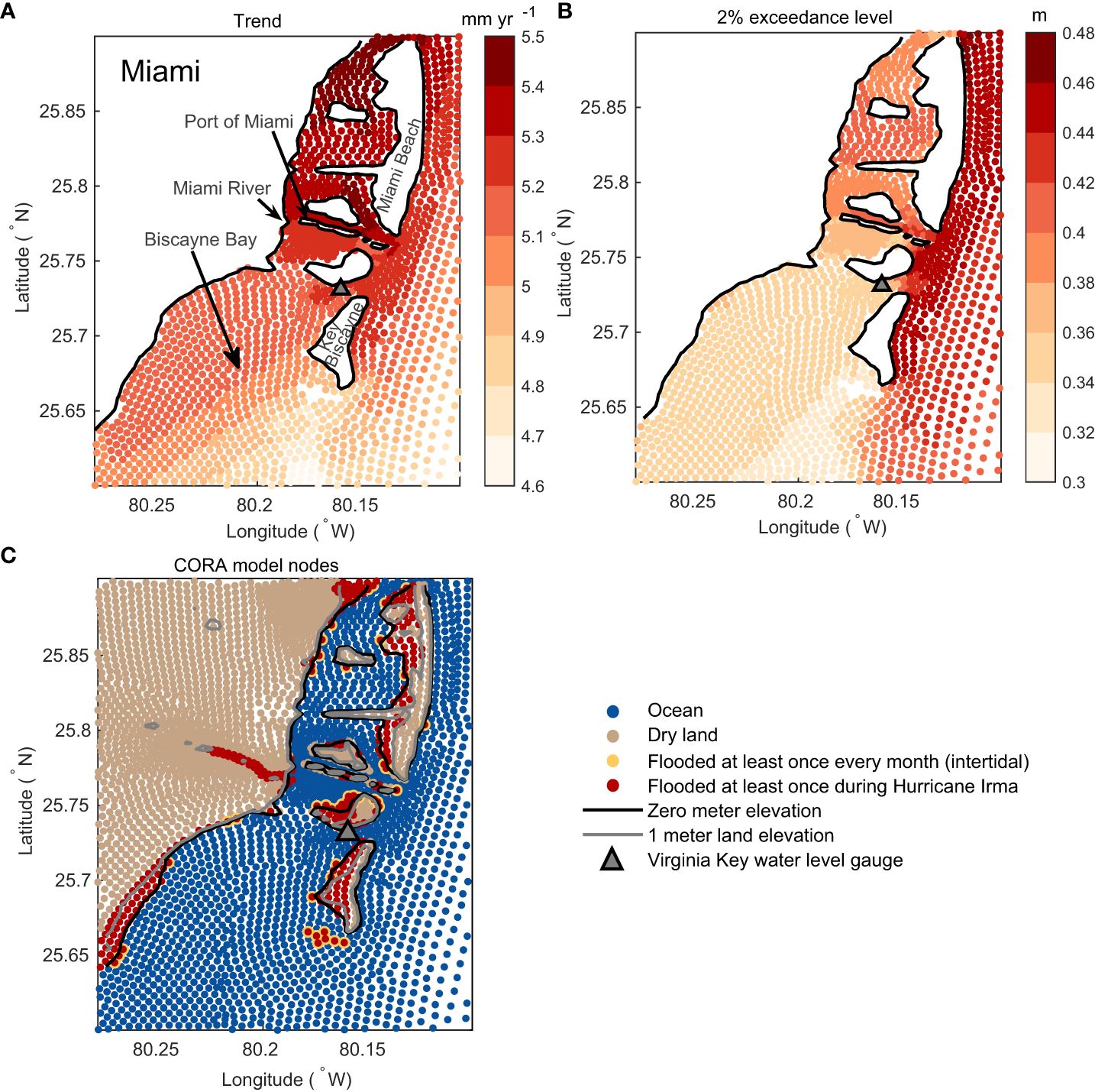
Figure 11 Application of CORA to assess coastal flooding in the Miami, FL area. CORA characteristics are shown at model nodes. (A) Trend from 1993–2020 (mm yr-1). Locations referred to in the text are labeled, and the Virginia Key water level gauge is indicated in each panel (triangle). (B) 2% exceedance of water levels with respect to MHHW (m). (C) Classification as ocean (blue), dry land (brown), flooded at least once per month (intertidal; yellow), or flooded at least once during Hurricane Irma (red; September 1–15, 2017). The flooding map also displays contour lines for the zero- and one- meter elevations (black and gray) of topographic-bathymetry in CORA.
The 2% exceedance level is also heterogeneous across the region (Figure 11B). Higher thresholds of the 2% exceedance are mostly in the open ocean areas such as adjacent to Miami Beach (greater than 0.44 m). Exceedance thresholds closer to 0.30 m are more common in Biscayne Bay, especially south of the port area. For comparison, the CORA characteristic closest to the Virginia Key water level gauge consists of a 0.352 m 2% exceedance level, which is only slightly higher than observed (0.333 m; Supplementary Table 1).
Another important application of CORA is assessing the regional flooding extent during past high-water level events. Our methodology for assessing flooding in the reanalysis, as explained in Section 2.3, is to categorize model nodes as either always wet (ocean), always dry (land), flooded at least once per month (intertidal), or occasionally flooded. It is the occasional flooding category that is most relevant from the perspective of assessing historical impacts associated with high-water levels. Hurricane Irma’s landfall, described in section 3.5, is the focus event of the regional case study. Storm surge associated with the hurricane was much higher closer to the landfall points (exceeding 2 m at Cudjoe Key and Marco Island according to surveys, (https://www.weather.gov/mfl/hurricaneirma), compared to the 1.11 m non-tidal residual observed at Virginia Key (Figure 9G). Since the current configuration of CORA demonstrates better capability at simulating realistic storm surges well away from the hurricane core of most severe winds, such as around water level gauges along the East Coast after Irma’s landfall (Figure 9), the domain of Figure 11 is well suited for a regional case study.
During Hurricane Irma, every model node in the Miami region that has flooded since 1979 (i.e., the “occasional flooding” category) was inundated for at least an hour, along with all the intertidal nodes (i.e., the red and yellow dots, respectively, in Figure 11C). The inundation pattern reveals areas particularly vulnerable to storm surge flooding, such as the bay side neighborhoods of Miami Beach. On the mainland, CORA depicts coastal flooding in the northern and southern parts of the case study domain as well as extending inland around the Miami River, although inundation in the latter area seems to be an artifact of the model topography and resolution because in reality the river is always connected to Biscayne Bay. Whereas in CORA, nodes near the Miami River are only sometimes flooded, as indicated by the red dots in Figure 11C. Other areas appear less susceptible to flooding since the model nodes remained dry during Hurricane Irma, which are mainly places of higher elevation. It is important to note that these flooding characteristics do not represent a worst-case scenario because the most severe hurricane winds were experienced outside of the region.
Miami is also experiencing chronic high-tide flooding, which is becoming more frequent with sea level rise (Wdowinski et al., 2016). Figure 12A shows that the number of days of extremely high-water levels have increased since the Virginia Key observations began in 1994, and that there is a pronounced annual cycle with an October peak. CORA closely resembles the observations. Employing the metric of flooding node-hours in CORA, we see similarity between the occurrences of extremely high-water levels and flooding (i.e., comparing Figures 12A, B). Highest sea levels are most often observed during August–October around Miami (e.g., Widlansky et al., 2020), which is also hurricane season and when most of the flooding occurs in CORA (Figure 12B). Like the increasing trend of extreme water levels (Figure 12A), there has also been a pronounced increase in monthly flood occurrence since 1979, with the most flooding in CORA happening during Hurricane Irma (Figure 12B). Furthermore, the six years with the most days of extremely high-water levels and flooded model nodes were all since 2015, which has been a period of frequent high-tide flooding for Miami (Sweet et al., 2018).
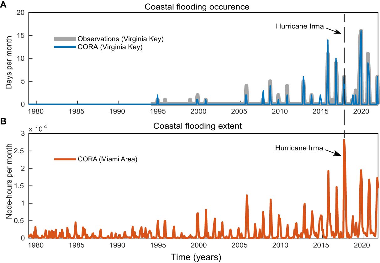
Figure 12 Coastal flooding metrics in the Miami, FL area. (A) Number of days per month that the daily maximum water level at Virginia Key was above the 2% exceedance threshold, according to observations (gray; since 1994) and CORA (blue). (B) Number of flooded node-hours per month, calculated as the cumulative sum of CORA nodes (orange) that were flooded in the domain shown in Figure 11. Nodes classified as ocean, land, or flooded once every month (intertidal) were excluded, highlighting the impact of extreme water level events such as during annual peaks of high tides or Hurricane Irma (vertical dashed line).
This study evaluates coastal water levels in NOAA’s CORA-GEC v0.9, as compared to NOAA’s NWLON observations and sea levels in the GLORYS12 reanalysis. This preliminary version of CORA spans 43 years of hourly water levels for the U.S. Gulf and East Coasts. CORA stands out due to its relatively high coastal resolution and thus accurate representation of many complex coastal features, its inclusion of inundation of coastal areas, and its assimilation of coastal water level observations to supplement the tidal and meteorologically forced responses that are explicitly included in the barotropic ADCIRC+SWAN model. We assessed CORA regarding coastal water levels on multiple timescales (i.e., considering the long-term trend and annual cycle as well as interannual, monthly, and hourly variability). Furthermore, we compared the performance of CORA to monthly and longer timescales of variability in GLORYS12, which is a global reanalysis that uses an entirely different approach to describing sea levels. Additional performance metrics included assessing tides and extremes in CORA compared to observations. We also considered applications such as using CORA to assess coastal flooding. Here, we summarize the results (Section 4.1) prior to discussing the implications and next steps (Section 4.2).
CORA closely matched water level observations, with slightly better performance at assimilated locations than at water level gauges that were not included in the assimilation. The satisfactory performance of CORA is attributable to the data assimilation method, which adjusts the ADCIRC water levels to observations. Regional performance differences are presumably related to the density of water level gauges available for assimilation, with areas having fewer observations showing lesser performance across most metrics (e.g., along the western Gulf Coast). CORA performance was consistently weakest at water level gauges located up coastal rivers, most likely due to inadequate resolution of these water bodies in the HSOFS mesh. In terms of performance hierarchy, CORA around assimilated water level gauges typically outperformed locations near non-assimilated water level gauges. Only considering the monthly and longer timescales of variability, including the long-term trends, CORA more closely matched observations compared to GLORYS12. While CORA adeptly captured storm surges, such as during Hurricanes Irma and Sandy, it encountered challenges with high-frequency variability at some locations on the Gulf Coast, which are possibly related to problems unexplored here such as resolving non-tidal diurnal cycles like land-sea breezes or other model characteristics like boundary forcings. CORA also tended to slightly underpredict tidal variability (i.e., having smaller amplitudes) and it exhibited phase errors at some locations, which requires further study to explain why. Both GLORYS12 and CORA effectively represented the annual cycle of coastal water levels. CORA also well represented extremely high-water level events. Most importantly, CORA excelled in tracking the observed rise in water levels above the 2% exceedance level, with a clear uptick in extremely high-water level days post-2015, especially for the Gulf Coast and areas like Miami that are experiencing more occurrences of flooding recently.
Overall, CORA offers a comprehensive description of water levels for the Gulf and East Coasts, providing insights for areas without extensive observations. The realism of CORA is achieved by the assimilation of observations from water level gauges, especially concerning long-term trends and monthly variability. CORA consistently matched observed water level trends, notably identifying a rise in days with extremely high-water levels at all of the locations considered. Likewise, we found the annual cycle of the clustering of extremely high-water levels is well represented, such as the typical occurrence during September and October for most locations along the Gulf and East Coasts.
Regarding chronic high-tide flooding, places like Miami have seen increased frequencies (Sweet et al., 2022). Around Miami, CORA realistically describes the observed rise in extremely high-water level days post-1994 and the marked increase in flood events since 2015. A focused study on the Miami region, centered on Hurricane Irma in 2017, demonstrated the utility of CORA in assessing coastal flooding characteristics. This case study emphasized the ability of using CORA to assess the combined effects of sea level rise and variability, as well as tides and storm surges, on coastal inundation events. Using CORA, we mapped areas prone to flooding in the Greater Miami area, highlighting its capability in assessing changing risks associated with higher sea levels. The findings present valuable data for adaptive and preventive strategies against sea level rise and extreme events.
CORA is a promising tool for assessing water level variations, tidal datums, and coastal flooding characteristics, especially in the context of rising sea levels. Its high-resolution coastal water level data is crucial for adapting to the challenges of sea level rise and extreme water levels caused by storm surges and other weather, climate, or tidal fluctuations. By assimilating observations from water level gauges, CORA captures behavior in trends and variability that could be caused by relative sea level rise, changing coastal ocean processes, and meteorological forcing. CORA’s use of the ADCIRC model, which is proficient in simulating storm surges, especially for large hurricanes and away from the central core of the strongest winds, makes it useful in coastal planning for future extremes. A more in-depth exploration into the effects of rising sea levels, return intervals of extreme water levels, regional flood thresholds, and in general the relationship between CORA and observations will be vital for informing future coastal strategies. The ADCIRC+SWAN simulations that comprise CORA have also generated hourly data sets of surface waves, which may be helpful for understanding the combined effects of water level and waves on coastal flooding (Aretxabaleta et al., 2023).
Looking forward, continued enhancements of CORA are ongoing. The next reanalysis version for the Gulf and East Coasts (NOAA CORA-GEC v1.0) includes more assimilated water level gauges, particularly in the western Gulf of Mexico. The subsequent version (v2) will incorporate higher-resolution atmospheric forcing from hurricanes to better capture extremely high storm surges (Bilskie et al., 2022). Additional improvement could also come from using vertical land motion observations (e.g., Wöppelmann and Marcos, 2016) to inform the calculation of water level correction surfaces between observation sources that are used in the assimilation process. Nevertheless, we found this preliminary version of CORA highly realistic as far as depicting monthly and hourly water level variability in areas without assimilated water level gauges, which suggests potential applications in what have been less observed and studied coastal regions. Plans are in place to expand CORA to the Pacific Ocean, which will likewise further the description of coastal water levels and flooding events in such regions (i.e., for the West Coast, Alaska, Hawaii, and U.S.-affiliated Pacific Islands).
CORA offers a new method for comprehensively analyzing the intertwined effects of historical sea level rise, water level variability, high tides, and storm surges on simulated coastal inundations. Particularly evident in areas like Miami, FL, which contends with these complex challenges on a recurrent basis, our assessment of CORA illuminates the nuances of coastal impacts (i.e., flooding as inferred by model nodes inundated with seawater). We showed that CORA resolves flooding occurrences affected by the long-term rise and annual cycle of sea level as well as more abrupt occurrences such as monthly water level anomalies, very high tides, and storm surges.
The Miami regional case study serves as a replicable approach for assessing flooding characteristics in other coastal zones, since it is accommodating to different topographies and weather patterns. However, the true efficacy of CORA’s depictions of coastal flooding hinges on validation against observed impacts. This validation data can span from detailed impact reports (e.g., using a methodology like in Hague et al., 2020) to visual confirmations via camera images (e.g., such as from NOAA’s Web Camera Observation Network; WebCOOS as reviewed in Dusek et al., 2019) or potentially satellite assessments. Furthermore, extra care will be needed in some regions to ascertain if the local relative water level rise depicted by CORA matches observations, which could be accomplished by utilizing additional observations of vertical land motions such as from InSAR and LiDAR measurements (Hurtado-Pulido, 2023). As such, with refinement and further verification, CORA could become pivotal for deciphering and addressing the multifaceted issues associated with coastal flooding.
In conclusion, CORA is a new dataset in coastal water level research, which may lead to advancements in the assessment and understanding of risks in a changing climate. The versatility and comprehensive approach of the reanalysis make it widely applicable for understanding and planning around coastal challenges. With its high-resolution water level data and broad applications, CORA stands as a foundation for future research about coastal environments, which will hopefully drive more informed decision-making in the face of rising sea levels and associated challenges.
Publicly available datasets were analyzed in this study. This data can be found here: (https://tidesandcurrents.noaa.gov/web_services_info.html https://data.marine.copernicus.eu/product/GLOBAL_MULTIYEAR_PHY_001_030/description https://uhslc.soest.hawaii.edu/Coastal_Reanalysis/).
LR: Conceptualization, Formal analysis, Investigation, Methodology, Visualization, Writing – original draft, Writing – review & editing. MW: Conceptualization, Methodology, Writing – original draft, Writing – review & editing. XF: Writing – review & editing. PT: Writing – review & editing. TA: Data curation, Writing – review & editing. GD: Supervision, Writing – review & editing. BB: Data curation, Writing – review & editing. RL: Data curation, Writing – review & editing. JC: Writing – review & editing. WB: Writing – review & editing. AK: Writing – review & editing. JH: Writing – review & editing. WS: Data curation, Writing – review & editing. AG: Writing – review & editing. PH: Writing – review & editing. JM: Writing – review & editing. JT: Data curation, Writing – review & editing.
The author(s) declare financial support was received for the research, authorship, and/or publication of this article. This assessment was primarily funded by NOAA’s support of the CIMAR-University of Hawaii Sea Level Center via the Center for Operational Oceanographic Products and Services as part of the National Ocean Service initiative for an improved National Coastal Data Information System.
The authors thank RENCI for making available the hourly water level output of NOAA’s CORA-GEC v0.9 (1979–2021) as well as CMEMS for providing the sea surface height data from GLORYS12. A large-language model (GPT-4 from OpenAI) was used to organize and edit parts of the writing.
Authors JC and JH are employed by Ocean Associates, Inc.
The remaining authors declare that the research was conducted in the absence of any commercial or financial relationships that could be construed as a potential conflict of interest.
All claims expressed in this article are solely those of the authors and do not necessarily represent those of their affiliated organizations, or those of the publisher, the editors and the reviewers. Any product that may be evaluated in this article, or claim that may be made by its manufacturer, is not guaranteed or endorsed by the publisher.
The Supplementary Material for this article can be found online at: https://www.frontiersin.org/articles/10.3389/fmars.2024.1381228/full#supplementary-material
Amaya D. J., Jacox M. G., Alexander M. A., Scott J. D., Deser C., Capotondi A., et al. (2023). Bottom marine heatwaves along the continental shelves of North America. Nat. Commun. 14, 1038. doi: 10.1038/s41467-023-36567-0
Aretxabaleta A. L., Sherwood C. R., Blanton B. O., Over J.-S. R., Traykovski P. A., Sogut E. (2023). “Temporal variability of runup and total water level on Cape Cod sandy beaches,” in Coastal Sediments 2023: The Proceedings of the Coastal Sediments 2023 (World Scientific). 267–281. doi: 10.1142/9789811275135_0024
Asher T. G., Luettich R. A., Fleming J. G., Blanton B. O. (2019). Low frequency water level correction in storm surge models using data assimilation. Ocean Model. 144, 101483. doi: 10.1016/j.ocemod.2019.101483
Bacopoulos P., Funakoshi Y., Hagen S. C., Cox A. T., Cardone V. j. (2009). The role of meteorological forcing on the St. Johns River (Northeastern Florida). J. Hydrol (Amst) 369, 55–70. doi: 10.1016/j.jhydrol.2009.02.027
Bilskie M. V., Asher T. G., Miller P. W., Fleming J. G., Hagen S. C., Luettich R. A. Jr. (2022). Real-time simulated storm surge predictions during hurricane Michael, (2018). Weather Forecast 37, 1085–1102. doi: 10.1175/WAF-D-21-0132.1
Bilskie M. V., Bacopoulos P., Hagen S. C. (2019). Astronomic tides and nonlinear tidal dispersion for a tropical coastal estuary with engineered features (causeways): Indian River lagoon system. Estuar. Coast. Shelf Sci. 216, 54–70. doi: 10.1016/j.ecss.2017.11.009
Booij N., Ris R. C., Holthuijsen L. H. (1999). A third-generation wave model for coastal regions: 1. Model description and validation. J. Geophys Res. Oceans 104, 7649–7666. doi: 10.1029/98JC02622
Bunya S., Dietrich J. C., Westerink J. J., Ebersole B. A., Smith J. M., Atkinson J. H., et al. (2010). A high-resolution coupled riverine flow, tide, wind, wind wave, and storm surge model for southern Louisiana and Mississippi. Part I: Model development and validation. Mon Weather Rev. 138, 345–377. doi: 10.1175/2009MWR2906.1
Buzzanga B., Bekaert D. P. S., Hamlington B. D., Kopp R. E., Govorcin M., Miller K. G. (2023). Localized uplift, widespread subsidence, and implications for sea level rise in the New York City metropolitan area. Sci. Adv. 9, eadi8259. doi: 10.1126/sciadv.adi8259
Buzzanga B., Bekaert D. P. S., Hamlington B. D., Sangha S. S. (2020). Toward sustained monitoring of subsidence at the coast using InSAR and GPS: An application in Hampton Roads, Virginia. Geophys Res. Lett. 47, e2020GL090013. doi: 10.1029/2020GL090013
Calafat F. M., Wahl T., Lindsten F., Williams J., Frajka-Williams E. (2018). Coherent modulation of the sea-level annual cycle in the United States by Atlantic Rossby waves. Nat. Commun. 9, 2571. doi: 10.1038/s41467–018-04898-y
Chi L., Wolfe C. L. P., Hameed S. (2018). Intercomparison of the Gulf Stream in ocean reanalyses: 1993–2010. Ocean Model. (Oxf) 125, 1–21. doi: 10.1016/j.ocemod.2018.02.008
Dusek G., Hernandez D., Willis M., Brown J. A., Long J. W., Porter D. E., et al. (2019). WebCAT: piloting the development of a web camera coastal observing network for diverse applications. Front. Mar. Sci. 6. doi: 10.3389/fmars.2019.00353
Egbert G. D., Erofeeva S. Y. (2002). Efficient inverse modeling of barotropic ocean tides. J. Atmos Ocean Technol. 19, 183–204. doi: 10.1175/1520-0426(2002)019<0183:EIMOBO>2.0.CO;2
Ezer T., Dangendorf S. (2022). The impact of remote temperature anomalies on the strength and position of the Gulf Stream and on coastal sea level variability: a model sensitivity study. Ocean Dyn 72, 223–239. doi: 10.1007/s10236-022-01500-4
Feng X., Widlansky M. J., Balmaseda M. A., Zuo H., Spillman C. M., Smith G., et al. (2024). Improved capabilities of global ocean reanalyses for analysing sea level variability near the Atlantic and Gulf of Mexico Coastal US. Front. Mar. Sci. 11, 1338626. doi: 10.3389/fmars.2024.1338626
Hague B. S., Murphy B. F., Jones D. A., Taylor A. J. (2020). Developing impact-based thresholds for coastal inundation from tide gauge observations. J. South. Hemisphere Earth Syst. Sci. 69, 252–272. doi: 10.1071/ES19024
Harvey T. C., Hamlington B. D., Frederikse T., Nerem R. S., Piecuch C. G., Hammond W. C., et al. (2021). Ocean mass, sterodynamic effects, and vertical land motion largely explain US coast relative sea level rise. Commun. Earth Environ. 2, 233. doi: 10.1038/s43247-021-00300-w
Hersbach H., Bell B., Berrisford P., Hirahara S., Horányi A., Muñoz-Sabater J., et al. (2020). The ERA5 global reanalysis. Q. J. R. Meteorological Soc. 146, 1999–2049. doi: 10.1002/qj.3803
Hurtado-Pulido C. (2023). InSAR and airborne LiDAR for monitoring slow vertical land motion. Nat. Rev. Earth Environ. 4, 679. doi: 10.1038/s43017-023-00442-9
Jean-Michel L., Eric G., Romain B. B., Gilles G., Angélique M., Marie D., et al. (2021). The copernicus global 1/12° Oceanic and sea ice GLORYS12 reanalysis. Front. Earth Sci. (Lausanne) 9. doi: 10.3389/feart.2021.698876
Juárez B., Stockton S. A., Serafin K. A., Valle-Levinson A. (2022). Compound flooding in a subtropical estuary caused by hurricane Irma 2017. Geophys Res. Lett. 49. doi: 10.1029/2022GL099360
Kolker A. S., Allison M. A., Hameed S. (2011). An evaluation of subsidence rates and sea-level variability in the northern Gulf of Mexico. Geophys Res. Lett. 38. doi: 10.1029/2011GL049458
Long X., Widlansky M. J., Spillman C. M., Kumar A., Balmaseda M., Thompson P. R., et al. (2021). Seasonal forecasting skill of sea-level anomalies in a multi-model prediction framework. J. Geophys Res. Oceans 126, e2020JC017060. doi: 10.1029/2020JC017060
Luettich R. A., Westerink J. J. (2004). Formulation and numerical implementation of the 2D/3D ADCIRC finite element model version 44. XX.
Ohenhen L. O., Shirzaei M., Ojha C., Kirwan M. L. (2023). Hidden vulnerability of US Atlantic coast to sea-level rise due to vertical land motion. Nat. Commun. 14, 2038. doi: 10.1038/s41467-023-37853-7
Piecuch C. G., Dangendorf S., Ponte R. M., Marcos M. (2016). Annual sea level changes on the North American northeast coast: Influence of local winds and barotropic motions. J. Clim 29, 4801–4816. doi: 10.1175/JCLI-D-16-0048.1
Piecuch C. G., Wadehra R. (2020). Dynamic sea level variability due to seasonal river discharge: A preliminary global ocean model study. Geophys Res. Lett. 47, e2020GL086984. doi: 10.1029/2020GL086984
Riverside Technologies, and Inc. AECOM (2015). Mesh development, tidal validation, and hindcast skill assessment of an ADCIRC model for the hurricane storm surge operational forecast system on the US gulf-atlantic coast. Rep. Prep. Natl. Ocean. Atmospheric Adm. Ocean Serv. Coast. Surv. Dev. Lab. Off. Coast. Surv 180. doi: 10.7921/G0MC8X6V
Sweet W. V., Dusek G., Obeysekera J. T. B., Marra J. J. (2018). Patterns and projections of high tide flooding along the US coastline using a common impact threshold. doi: 10.7289/V5/TR-NOS-COOPS-086
Sweet W. V., Hamlington B. D., Kopp R. E., Weaver C. P., Barnard P. L., Bekaert D., et al. (2022). Global and regional sea level rise scenarios for the United States: Updated mean projections and extreme water level probabilities along US coastlines. Natl. Oceanic Atmospheric Administration. doi: 10.7289/v5/tr-nos-coops-083
Sweet W. V., Park J. (2014). From the extreme to the mean: Acceleration and tipping points of coastal inundation from sea level rise. Earths Future 2, 579–600. doi: 10.1002/2014EF000272
Wahl T., Jain S., Bender J., Meyers S. D., Luther M. E. (2015). Increasing risk of compound flooding from storm surge and rainfall for major US cities. Nat. Clim Chang 5, 1093–1097. doi: 10.1038/nclimate2736
Wdowinski S., Bray R., Kirtman B. P., Wu Z. (2016). Increasing flooding hazard in coastal communities due to rising sea level: Case study of Miami Beach, Florida. Ocean Coast. Manag 126, 1–8. doi: 10.1016/j.ocecoaman.2016.03.002
Westerink J. J., Luettich R. A., Feyen J. C., Atkinson J. H., Dawson C., Roberts H. J., et al. (2008). A basin- to channel-scale unstructured grid hurricane storm surge model applied to southern Louisiana. Mon Weather Rev. 136, 833–864. doi: 10.1175/2007MWR1946.1
Widlansky M. J., Long X., Balmaseda M. A., Spillman C. M., Smith G., Zuo H., et al. (2023). Quantifying the benefits of altimetry assimilation in seasonal forecasts of the upper ocean. J. Geophys Res. Oceans 128, e2022JC019342. doi: 10.1029/2022JC019342
Widlansky M. J., Long X., Schloesser F. (2020). Increase in sea level variability with ocean warming associated with the nonlinear thermal expansion of seawater. Commun. Earth Environ. 1, 9. doi: 10.1038/s43247-020-0008-8
Wöppelmann G., Marcos M. (2016). Vertical land motion as a key to understanding sea level change and variability. Rev. Geophysics 54, 64–92. doi: 10.1002/2015RG000502
Keywords: Coastal Ocean Reanalysis (CORA), ADCIRC model, water level variability, storm surge, coastal flooding risk
Citation: Rose L, Widlansky MJ, Feng X, Thompson P, Asher TG, Dusek G, Blanton B, Luettich RA Jr., Callahan J, Brooks W, Keeney A, Haddad J, Sweet W, Genz A, Hovenga P, Marra J and Tilson J (2024) Assessment of water levels from 43 years of NOAA’s Coastal Ocean Reanalysis (CORA) for the Gulf of Mexico and East Coasts. Front. Mar. Sci. 11:1381228. doi: 10.3389/fmars.2024.1381228
Received: 03 February 2024; Accepted: 14 May 2024;
Published: 03 June 2024.
Edited by:
Deborah Idier, Bureau de Recherches Géologiques et Minières, FranceReviewed by:
Davina Passeri, United States Department of the Interior, United StatesCopyright © 2024 Rose, Widlansky, Feng, Thompson, Asher, Dusek, Blanton, Luettich, Callahan, Brooks, Keeney, Haddad, Sweet, Genz, Hovenga, Marra and Tilson. This is an open-access article distributed under the terms of the Creative Commons Attribution License (CC BY). The use, distribution or reproduction in other forums is permitted, provided the original author(s) and the copyright owner(s) are credited and that the original publication in this journal is cited, in accordance with accepted academic practice. No use, distribution or reproduction is permitted which does not comply with these terms.
*Correspondence: Linta Rose, bGludGFyQGhhd2FpaS5lZHU=; Matthew J. Widlansky, bXdpZGxhbnNAaGF3YWlpLmVkdQ==
Disclaimer: All claims expressed in this article are solely those of the authors and do not necessarily represent those of their affiliated organizations, or those of the publisher, the editors and the reviewers. Any product that may be evaluated in this article or claim that may be made by its manufacturer is not guaranteed or endorsed by the publisher.
Research integrity at Frontiers
Learn more about the work of our research integrity team to safeguard the quality of each article we publish.