Reconstructing the sound speed profile of South China Sea using remote sensing data and long short-term memory neural networks

Introduction: Sound waves are refracted along the direction of their propagation owing to spatial and temporal fluctuations in the speed of sound in seawater. Errors are compounded when sound speed profiles (SSPs) with low precision are used to detect and locate distant underwater targets because an accurate SSP is critical for the identification of underwater objects based on acoustic data. Only sparse historical spatiotemporal data on the SSP of the South China Sea are available owing to political issues, its complex atmospheric system, and the unique topography of its seabed, because of which frequent oceanic movements at the mesoscale affect the accuracy of inversion of its SSP.

Method: In this study, we propose a method for the inversion of the SSP of the South China Sea based on a long short-term memory model. We use continuous-time data on the SSP of the South China Sea as well as satellite observations of the height and temperature of the sea surface to make use of the long-term and short-term memory-related capacities of the proposed model.

Result: It can achieve highly accurate results while using a small number of samples by virtue of the unique structure of its memory. Compared with the single empirical orthogonal function regression method, the inversion accuracy of this model is improved by 24.5%, and it performed exceptionally well in regions with frequent mesoscale movements.

Discussion: This enables it to effectively address the challenges posed by the sparse sample distribution and the frequent mesoscale movements of the South China Sea.

1 Introduction

The sound speed profile (SSP) is an important oceanic parameter that is used in a variety of marine acoustic applications, such as underwater target identification, underwater communication, and marine environmental monitoring (Teymorian et al., 2009; Xu et al., 2013; Liu L. et al., 2021; Luo et al., 2022; Su et al., 2022; Zhan et al., 2023). The speed of sound varies significantly even in adjacent areas of the sea due to the complexity and variability of the marine environment. Even though it is the largest territorial marine area in China, research on the characteristics of the South China Sea began relatively late owing to political and territorial issues. According to the most recent map of the global seabed published in 2023, only about one-third of the seabed of the South China Sea has been surveyed thus far. The speed of sound is among the most significant factors that currently limit the accuracy of detection of underwater targets. Researchers have spent a considerable amount of time and effort in reducing errors in the speed of sound and ray tracing to improve the accuracy of detection of underwater engineering (Xu et al., 2005). By denoising the signal and optimizing the algorithm, the researchers reduce the impact of low precision sound speed on underwater engineering applications (Li et al., 2022b; Li et al., 2022a; Li et al., 2022c).

Researchers have identified links between the parameters of profiles of the sea surface and subsurface, and have proposed a number of methods to satisfy the increasingly stringent demands on the precision and speed of marine data in ocean engineering (Carnes et al., 1990; Stammer, 1997; Wunsch, 1997; Liu Y. et al., 2021; Yan et al., 2022). Remote sensing technology can be used to capture near-real-time and large-scale data on the ocean surface, where this enables the rapid acquisition of SSPs in the ocean. The corresponding techniques have provided us with a better understanding of the underlying processes of deep ocean motion (Klemas and Yan, 2014). Initial research in the area used linear approaches to infer the SSPs from the parameters of remote sensing data obtained from satellites. The empirical orthogonal function (EOF) was used as the basic function in this process. It plays a critical role in limiting the dimensionality of the parameters, reducing the computational load during inversion, and filtering out minor errors during computations (LeBlanc and Middleton, 1980). Carnes discovered that the parameters of satellite remote sensing, such as the height and temperature of the sea surface, are essential for inferring the temperature profiles of water bodies (Carnes et al., 1994). This insight led to the development of the EOF-based method of inversion called the single empirical orthogonal regression function (sEOFr). Chen et al. used this approach to invert the global SSPs, and showed that the sEOFr method can be used to directly infer the SSP without converting the temperature (Chen et al., 2018). The United States Navy successfully used this method in a modular ocean data assimilation system (Rahaman et al., 2016). While these methods are effective, the relationship between the parameters of the sea are not linear, and errors are thus inevitably generated when using the linear sEOFr method to describe the physical relationship between the relevant parameters. Jain found that errors in data on the inverted SSP primarily converged at depths ranging from 40 to 125 m owing to intense oceanic movements in the South China Sea at the mesoscale. Linear methods struggle to resolve such parametric relationships (Jain and Ali, 2006).

Su et al. used machine learning-based techniques instead of linear methods to investigate the relationship between parameters of the ocean. They used classical machine learning methods and support vector regression to predict global ocean temperatures beyond 1000 m by using satellite remote sensing data (Su et al., 2015; Su et al., 2019). Machine learning methods not only have advantages over conventional techniques in inferring the temperature profiles, but also in inferring the SSP. Ou used a tree-based algorithm along with parameters of remote sensing to invert the SSP, and reported a 25% improvement in the accuracy of the outcomes (Ou et al., 2022). Furthermore, Li et al. successfully inverted the SSP of the South China Sea by using a non-linear approach based on self-organizing maps (Li et al., 2021).

Inverting the SSP by using machine learning methods in conjunction with the parameters of remote sensing remarkably improves the accuracy of the results. However, the sEOFr method as well as other currently used techniques require a large number of training samples to deliver accurate results, and deliver subpar performance in the presence of intense activity at the mesoscale. The underwater terrain of the South China Sea is characterized by a deep ocean basin surrounded by sloped land, where the southwest slopes are higher than those in the northeast. The water bodies in the central and northern basins of the sea exchange water with the Pacific Ocean via certain straits, while the southern shelf near the Equator exchanges water with the Java Sea via the Malay Peninsula and the Borneo passage. Hence, the South China Sea contains water masses with varied origins and, thus, different hydrological characteristics. The tropical oceanic climate of the region is notable for its alternating rotation of southwestern winds in the summer and northeastern winds in the winter, and this leads to the formation of a complex atmospheric system. Scant historical data on the South China Sea have been accumulated for political reasons, which makes it challenging to invert its SSP. This task is rendered more onerous owing to the complex mechanism of disturbance in the SSP caused by the atmospheric system and the unique terrain of the area.

The authors of this study propose a long short-term memory (LSTM) based algorithm to invert the SSP of the South China Sea by using the parameters of remote sensing. The linear constraints in the relation between the parameters of the surface and the ocean can be eliminated by introducing an artificial neural network. The unique memory structure of the LSTM network can be used to overcome the problem of the small number of samples as well as the complex mechanism of disturbance in the SSP in the area. We used the root mean-squared error (RMSE) and mean absolute error (MAE) to compare the proposed method with the sEORr method, and the results showed that it is more accurate, and requires a smaller number of data samples. Moreover, it delivers better performance in regions featuring greater disturbances.

2 Data

We chose the South China Sea as the location for the inversion of the SSP because it is particularly challenging in this regard owing to frequent oceanic movements in the region. We used the LSTM model in conjunction with remote sensing data to precisely invert the SSP. We used a variety of datasets, including remote sensing data to create a regression database, data from Argo to construct SSP fields under water, and WOA18 data to compute the background profiles. The data used here had been collected from 2009 to 2018.

The remote sensing dataset included information on the height and temperature of the sea surface from the L4 satellite observation product of the Copernicus project (https://resources.marine.copernicus.eu). The data had a one-day temporal resolution and a spatial resolution of 0.25°. The experiments involved computing the mean values of all the data on the height and temperature of the sea surface, and then deriving the sea surface height anomaly and the sea surface temperature anomaly from them to establish a regression database.

The Argo data were obtained from the Argo dataset on the global ocean (2009–2018), and were preprocessed to remove anomalous data while retaining data within the undistorted range of depth of 5–1000 m. The Argo data had been obtained by using Argo floats, which are capable of simultaneously measuring the temperature and salinity profiles of seawater. The SSP is a function of the temperature, salinity, and hydrostatic pressure, and can be calculated by using the empirical formula proposed by Del Grosso to determine the SSP (Del Grosso, 1974). Figure 1 shows the entire set of 3,883 samples used for this study. A segment of continuously measured data was selected to train and test the LSTM model, and was called the TEST dataset. It is represented by the black dots in Figure 1. The TEST dataset contained 269 samples that were arranged chronologically from July 9, 2014 to April 2, 2015.

Figure 1

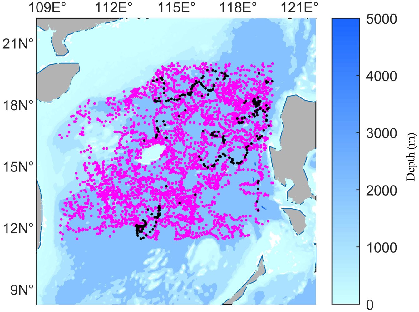
Figure 1 Distribution of the experimental samples (the black dots are test samples and the rest are training samples).

The background profiles represented the stable and unchanging portion of the SSP, and are typically represented by the average values of all profiles. WOA18 data were used to calculate the background profiles in this study. These data were obtained from the National Oceanic and Atmospheric Administration’s National Centers for Environmental Information (https://www.nodc.noaa.gov/OC5/woa18/), and combined multiple datasets with measurements of the temperature, salinity, density, and other climate-averaged data from various global oceanic regions. The experiments made use of annually averaged data that were obtained at a spatial resolution of 0.25° ×0.25°from 2009 to 2018. In this paper, WOA data at the center point of the inversion region (15.5°N, 145.5°E) is selected as the background profile of this experiment, and the specific profile values are shown in Figure 2.

Figure 2

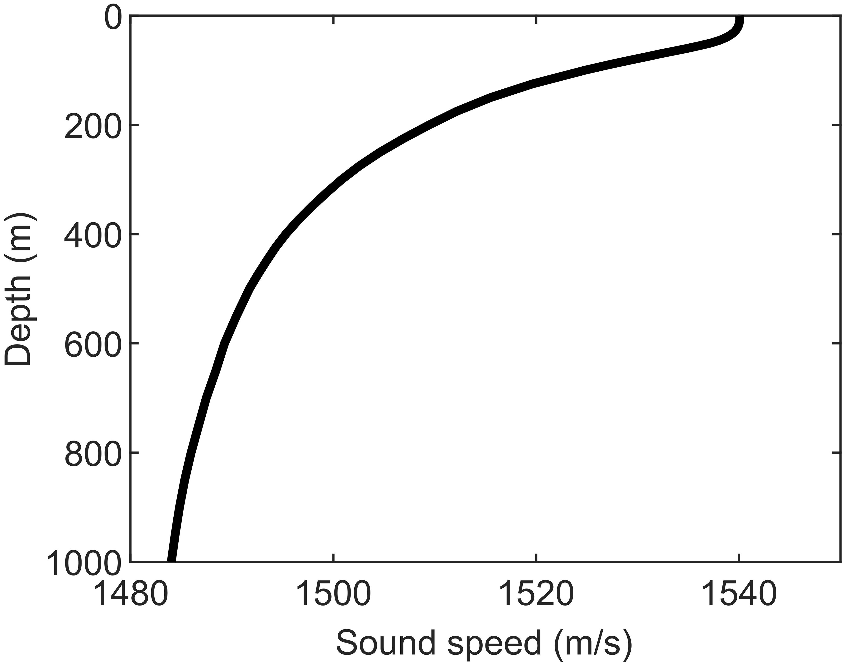
Figure 2 Background profile.

3 Inversion of sound speed profiles

3.1 Construction of the basis function of the sound speed profile

Basis functions serve as a method of dimension reduction in the context of the problem of inverting the field of sound speed, and their accuracy has a significant influence on the precision of calculation of the field of sound speed. Figure 3 shows how to extract the basis function EOF from the historical data and obtain the corresponding disturbance coefficient. Finally, the reliability of SSP reconstructed by perturbation coefficient is verified. The shift of the ssp sample relative to the mean is called a disturbance. ${\text{SSP}}_{\text{Argo SSP}}^{\text{disturbance}}$represents the difference between the SSP field and the background profile, and is denoted by the perturbation in the field of the sound speed.

Figure 3

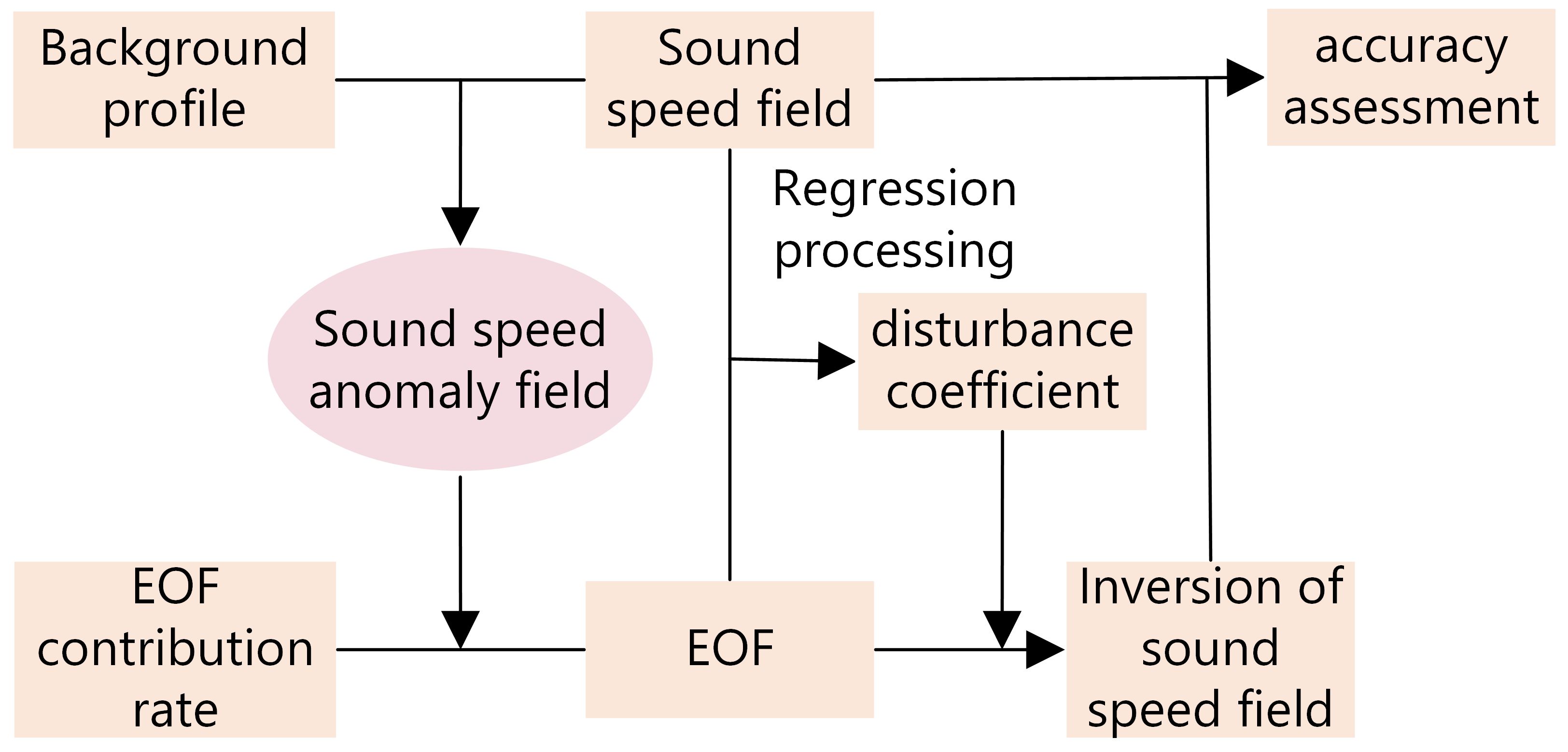
Figure 3 Flowchart of preprocessing of the sound speed profile.

$\begin{array}{ll}\text{COV}\times \text{EOF}=\text{EOF}\times \text{λ}& (1)\end{array}$

We calculated the covariance matrix, COV, of the disturbance in the speed field and performed orthogonal decomposition by Equation 1. In this equation, EOF represents the basis functions of the SSP while λ stands for the eigenvalue matrix.

The EOF can be used to identify the primary modes of changes in water. The role of EOF is to reduce the dimensionality of the data, reducing the amount of computation while avoiding the introduction of additional noise. Figure 4 shows the amplitudes of the first 5 orders of EOF for this experiment. It shows that most of the disturbance in the water is concentrated in the depth of 100–200m, and there is basically no disturbance below 500m.It is widely assumed that a contribution of 95% can represent a majority of disturbances in water. Based on $\text{λ}$, the contribution rate of each mode of EOF can be calculated. Figure 5 illustrates the distribution of the contributions of the first five modes, accounting for 70.69%, 16%, 4.86%, 3.30%, and 1.58% of the total, for an overall contribution of 96.43%. We thus used the first five orders of the EOF as the basis functions for the experiments in this study.

Figure 4

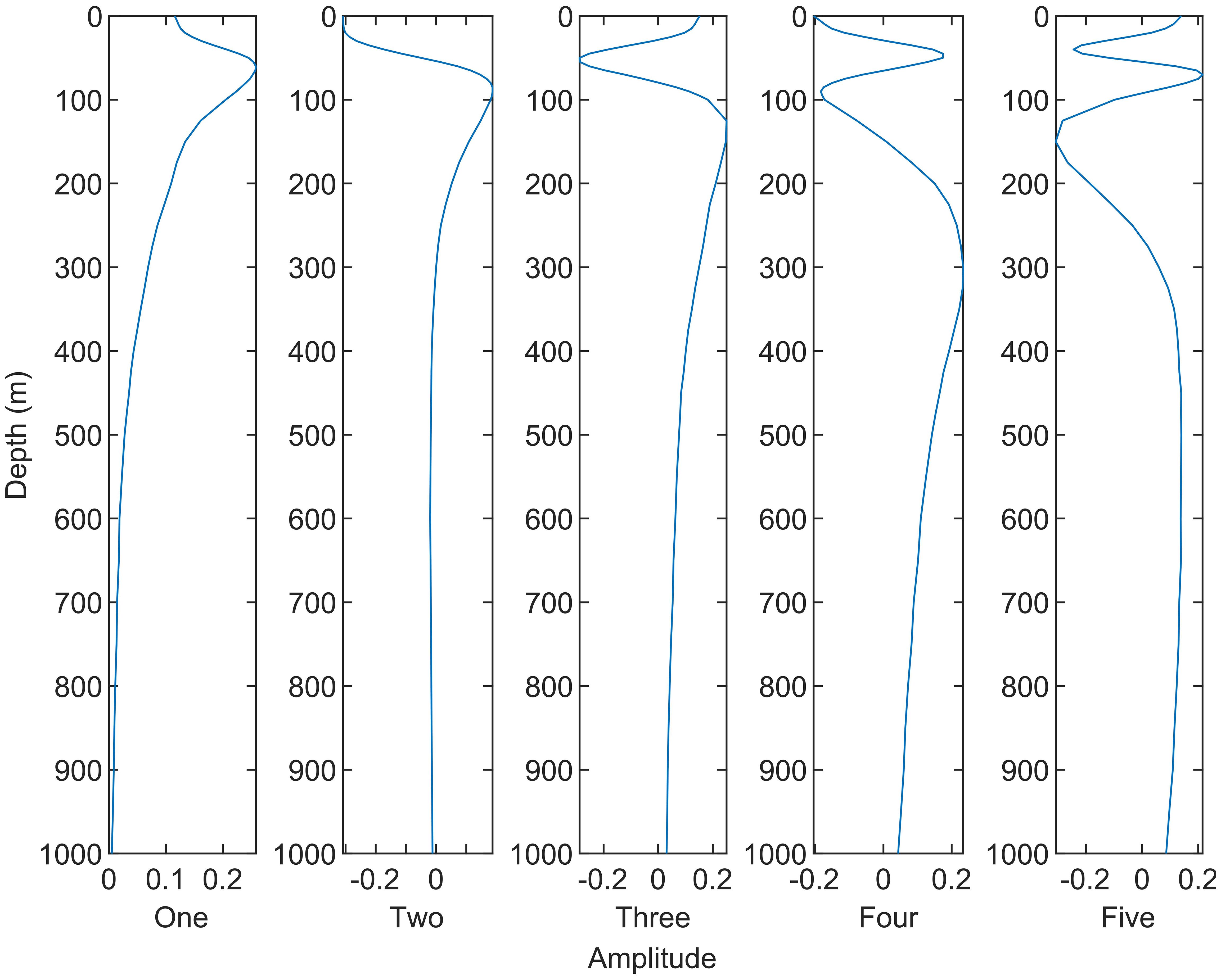
Figure 4 Amplitude of the first 5 EOFs.

Figure 5

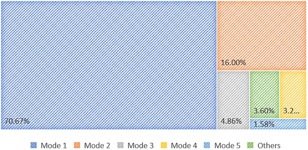
Figure 5 Distributions of contributions of the basis function.

The least square method is used to fit the EOF and the sound speed field, and the disturbance coefficient is obtained. Then the perturbation coefficient and EOF are used to calculate the sound speed field to ensure the accuracy of the perturbation coefficient and EOF. A comparison between the reconstructed values obtained from this inversion and the actual values yielded an RMSE of 0.62 m/s. Such a small error indicates that the shape functions of the EOF adequately represented a significant part of the variance in disturbances within the region, thus ensuring a relatively accurate reconstruction.

3.2 Single empirical orthogonal regression function

The parameters of remote sensing at the same time and at the same location can be linearly related to those of the seabed. We created a regression database by using a large amount of historical data to establish a regression relationship among the temperature of the sea surface, its height, and the coefficients of perturbation.

$\begin{array}{ll}{\text{ω}}_{\text{i},\text{j}}=\text{α}+\text{β}\times \text{A}+\text{γ}\times \text{B}+\text{δ}\times \text{A}\times \text{B}& (2)\end{array}$

This procedure entailed fitting a linear equation by using the database, expressed as Equation 2. where ${\text{ω}}_{\text{i},\text{j}}$ denotes the $j$-th order coefficient of perturbation of the $i$-th sample, and A and B denote anomalies in the height and the temperature of the sea surface, respectively. Linear fitting was used to obtain the coefficients $\text{α},\text{ β},\text{ γ},\text{ and δ}$. The corresponding coefficients of perturbation were obtained by entering the parameters of remote sensing, and the field of sound field of the South China Sea could then be inverted. The sEOFr method is based on linear regression between the parameters of remote sensing and the coefficients of projection. This linear relationship is derived from statistical results obtained from a large number of samples collected from the sea. In general, the errors tended to be concentrated in cases involving prominent differences between individual characteristics and statistical features.

3.3 Inversion of sound speed profile by using LSTM model

Given that the relationships between the parameters of the ocean were not purely linear, error was concentrated in regions featuring conspicuous perturbations. We propose a method of SSP inversion based on the LSTM neural network to improve the accuracy of inversion. Hochreiter created the LSTM model, which is an iterative version of the RNN model (Hochreiter and Schmidhuber, 1997). The LSTM model contains a memory cell that enables it to incorporate historical data, assess the relevance of information, improve its retention of valid information, filter out irrelevant information, and generate an output (Jain et al., 2019; Khataei Maragheh et al., 2022).

Figure 6 shows the structure of the LSTM model. It is composed of a forget gate, an input gate, and an output gate. Based on the previous output and the current input, the forget gate decides whether to forget the previous information or add it to the current memory cell.

Figure 6

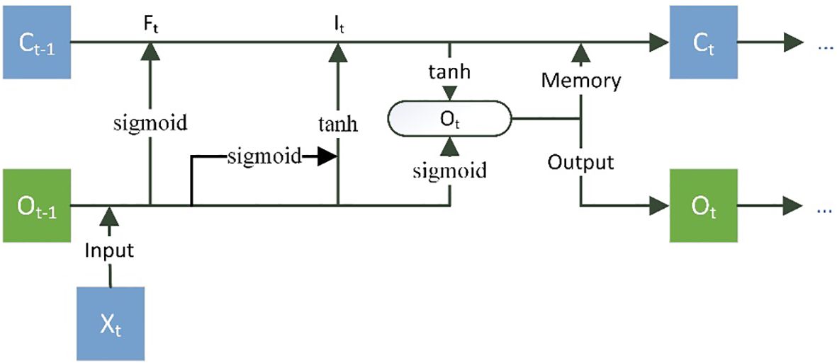
Figure 6 Diagram of the LSTM model.

$\begin{array}{ll}{\text{F}}_{\text{t}}=\text{sigmoid}({\text{ϵ}}_{\text{f}}[{\text{O}}_{\text{t}-1},{\text{X}}_{\text{t}}]+{\text{θ}}_1){*\text{C}}_{\text{t}-1}& (3)\end{array}$

Equation 3 is the calculation principle of the forgetting gate. where ${\text{O}}_{\text{t}-1}$denotes the output data from the previous time step, ${\text{X}}_t$denotes the input data in the current time step, ${\text{C}}_{\text{t}-1}$denotes the memory cell of the previous time step, and sigmoid denotes the activation function used to screen information within the range (0,1). In this experiment, Xt refers to sea surface height data and sea surface temperature data. ${\text{θ}}_1$is a bias term that serves as an additional input for the corresponding neuron, and ${\text{ϵ}}_f$is the weight that represents the strength of the connection between units of the corresponding gate. The forget gate allows for the reinforcement of useful information while discarding irrelevant information, thus avoiding such problems as gradient explosion and the vanishing gradient that are caused by multiple iterations (Wang et al., 2020).

$\begin{array}{ll}{\text{I}}_{\text{t}}=\text{ sigmoid}({\text{ϵ}}_{\text{i}}[{\text{O}}_{\text{t}-1},{\text{X}}_{\text{t}}]+{\text{θ}}_2)*\text{tanh}({\text{ϵ}}_{\text{c}}[{\text{O}}_{\text{t}-1},{\text{X}}_{\text{t}}]+{\text{θ}}_3)+{\text{F}}_{\text{t}}& (4)\end{array}$

The input gate is used to validate information and update the memory cell ${\text{I}}_{\text{t}}$, which is calculated by Equation 4. where ${\text{ϵ}}_{\text{i}}{\text{ and ϵ}}_c$are weights, and ${\text{θ}}_2{\text{ and θ}}_3$are bias terms that are used with the hyperbolic tangent (tanh) activation function in the interval (-1, 1). The tanh function is used by the input gate to generate the memory cell for the current time step. There are two steps involved, the first is to control the value between (0, 1) by the σ function, and the second is to generate the cell state of the current input by a tanh function. Following this, the information is filtered and added to the memory cell from the previous time step to enable it to be updated.

$\begin{array}{ll}{\text{O}}_{\text{t}}=\text{ sigmoid}({\text{ϵ}}_{\text{o}}[{\text{O}}_{\text{t}-1},{\text{X}}_{\text{t}}]+{\text{θ}}_4)*\text{tanh}({\text{I}}_{\text{t}})& (5)\end{array}$

The output gate determines the output data and passes them to the next time step. The relevant calculation formula is shown in Equation 5. where ${\text{ O}}_{\text{t}}$represents the output from the hidden layer at time $t$, ${\text{ϵ}}_o$is its weight, and ${\text{θ}}_4$is a bias term. In this experiment, Ot is the EOF coefficient.

Figure 7 shows the training and testing of the LSTM model. S1-S269 in Figure 5 is the input data corresponding to sample No. 1–269 in the test example, including sea surface height data and sea surface temperature data. “C1-C269” refers to the output data corresponding to samples 1–269 in the test sample, and the output data is the EOF coefficient. We used the parameters of remote sensing as the input to the model and obtained the coefficients of perturbation as the output in the experiments. To train the LSTM neural network model, the parameters of remote sensing were fed to the input gate. The specific operational procedure entails utilizing the actual values of samples 1–8 as inputs for training the model, while the predicted value of sample 9 is generated as the output. Subsequently, the model undergoes training with the true values of samples 2–9, leading to the prediction of the value for sample 10. This iterative process continues until the model output yields the predicted value for sample 269, thereby culminating in the prediction of values for samples 9 through 269.The model was continually adjusted by being trained on temporally sequential data, and the RMSE was used as the loss function. Following this, the parameters of remote sensing for the next time step were entered to yield the corresponding coefficients of perturbation for SSP inversion. The EOF coefficient of the output is tested and then brought into Equations 6, 7. The SSP based on LSTM model inversion is calculated. The SSP can be expressed as the background profile plus the disturbance value. The background profile was obtained from WOA data. The sound speed disturbance value is obtained by multiplying the EOF coefficient calculated by the model with the EOF extracted previously. M is the order of EOF selected in the experiment.

Figure 7

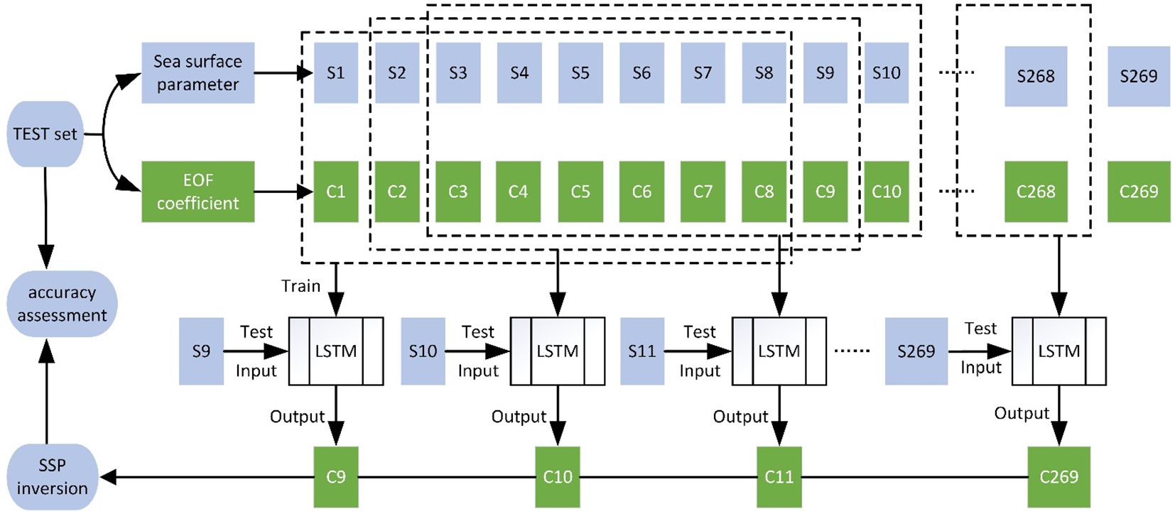
Figure 7 Flowchart of inversion of the field of sound speed by using the LSTM model.

$\begin{array}{ll}SSP=\widehat{SSP}+SS{P}^{\text{disturbance}}& (6)\end{array}$

$\begin{array}{ll}SS{P}^{\text{disturbance}}=\sum _{j=1}^M{\text{ω}}_{\text{j}}EOF(j),M\in (1,2,3,4,5)& (7)\end{array}$

LSTM model is a nonlinear model, which has the advantage of preventing gradient vanishing and gradient explosion when dealing with long series data. Compared with linear sEOFr model, it is more suitable for complex ocean dynamic model. The use of the LSTM model allowed us to apply an incremental approach to invert the sound field of the TEST dataset. SSP has a strong time correlation, LSTM algorithm can learn the correct time pattern by memorizing the structure, and predict the subsequent data. When we used a continuous temporal duration of eight for training, the model was able to maintain a relatively high accuracy of training with a small number of training samples in the experiment. This method reduced the reliance of the model on a large number of samples while maintaining a high accuracy.

4 Results and analysis of inversion

4.1 Evaluation of results of inversion of sEOFr and LSTM

Temperature, salinity, and pressure are the primary determinants of the speed of sound. Its speed increases by approximately 4.2 m/s for every 1°C increase in the temperature of water, an increase of 0.1% in the salinity of water corresponds to that of 0.13 m/s in the speed of sound, while a 1 atm increase in water pressure corresponds to a 0.17 m/s increase in the sound speed.

From the sea surface to the 100 m underwater, the seawater is referred to as the mixed layer because it receives sunlight exposure, allowing it to absorb solar heat, resulting in relatively higher temperatures and minor temperature variations. The thermocline is a layer located approximately 100 m beneath the mixed layer. The temperature drops rapidly with depth at this thermocline. The thermocline in the South China Sea, which is located in a medium-to-low-latitude region, was assumed to be 100 m deep in our experiments. The rapid change in the temperature of this layer led to prominent fluctuations in the sound speed. Furthermore, eddies at the mesoscale, internal waves, and other oceanic activities occur frequently in this area (Hu et al., 2000; Sun et al., 2020). The complex combination of these factors contributes to the difficulty of inverting the SSP. Figure 8 shows the variation of the error in the direction of depth. The factors mentioned earlier cause the error in the model inversion results to be concentrated at a depth of about 100 m. The variance in the temperature gradually stabilized below the thermocline, thus reducing the errors in modeling. In this study, Figure 9 shows the average inversion errors of the two models in different seasons. The results indicate that the errors of the LSTM model increase in July, December, and April, corresponding to seasons with substantial variations. This is attributed to the poor performance of the LSTM model during seasonal changes, as it only utilizes the preceding 8 time steps of predicted samples for training. As the seasonal transitions stabilize, the errors of the LSTM model decrease. In contrast, the sEOFr model, being based on a linear model statistically derived from annual sound speed profile data, exhibits larger errors during winter due to significant sound speed disturbances.

Figure 8

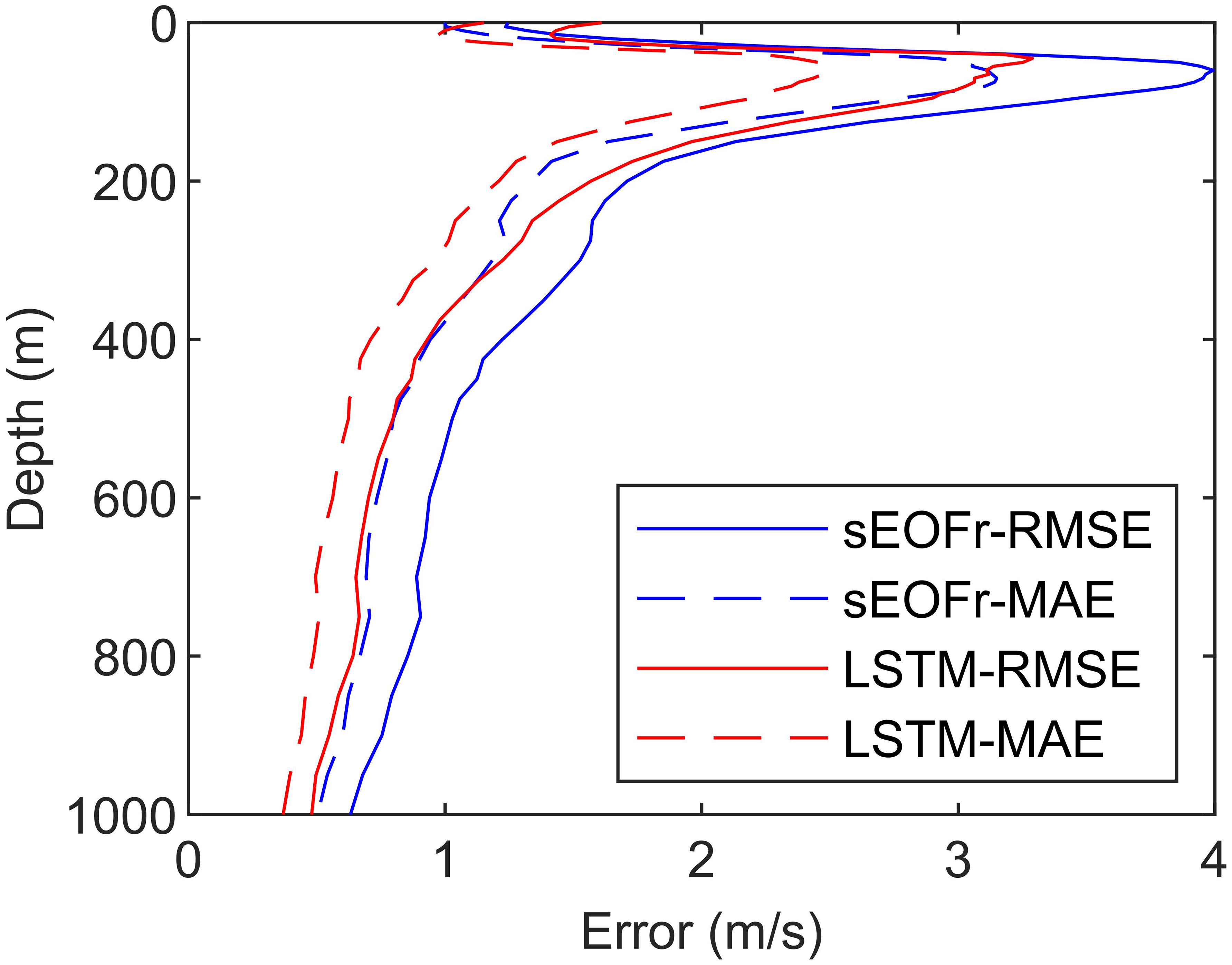
Figure 8 Distribution of error incurred by the model with depth below the sea surface.

Figure 9

Figure 9 The distribution of errors in different seasons. (from July 9, 2014 to April 3, 2015).

Figure 10 shows the spatial distributions of errors in the fields of sound obtained by the two models. The average error of the LSTM model was 1.76 m/s while that of the sEOFr model was 2.33 m/s. Errors incurred by the latter were mostly concentrated in the blue-framed area in the figure (119° E–119.5° E, 18° N–18.5° N). Mesoscale eddies were frequently active at this location, especially with intense Ekman aspiration activity (Xiao et al., 2013) that led to the mixing of deep and surface waters to thicken the mixed layer of the ocean. However, the sound speed field in the sea area where the thickness of the mixed layer is large will produce a large disturbance. Figure 11 shows the spatial distribution of sound speed disturbance values. The area in which error was concentrated and that in which the disturbance was large significantly overlapped, indicating that the disturbance-related values were a key factor influencing the accuracy of inversion of the model. The RMSE of the linear sEOFr model in the error concentration area is 3.83 m/s, 1.50 m/s higher than the overall RMSE, and the accuracy is reduced by 64% The RMSE of the LSTM model is 2.16m/s, which is only 0.40m/s higher than the overall RMSE, and the accuracy is only reduced by 23%.In this area, the inversion accuracy of LSTM model is improved by 43.6% compared with sEOFr model. It also shows that the linear model was unable to handle disturbances in this area, where this led to the concentration of error, while the LSTM model continued to deliver better performance and higher robustness in such scenarios.

Figure 10

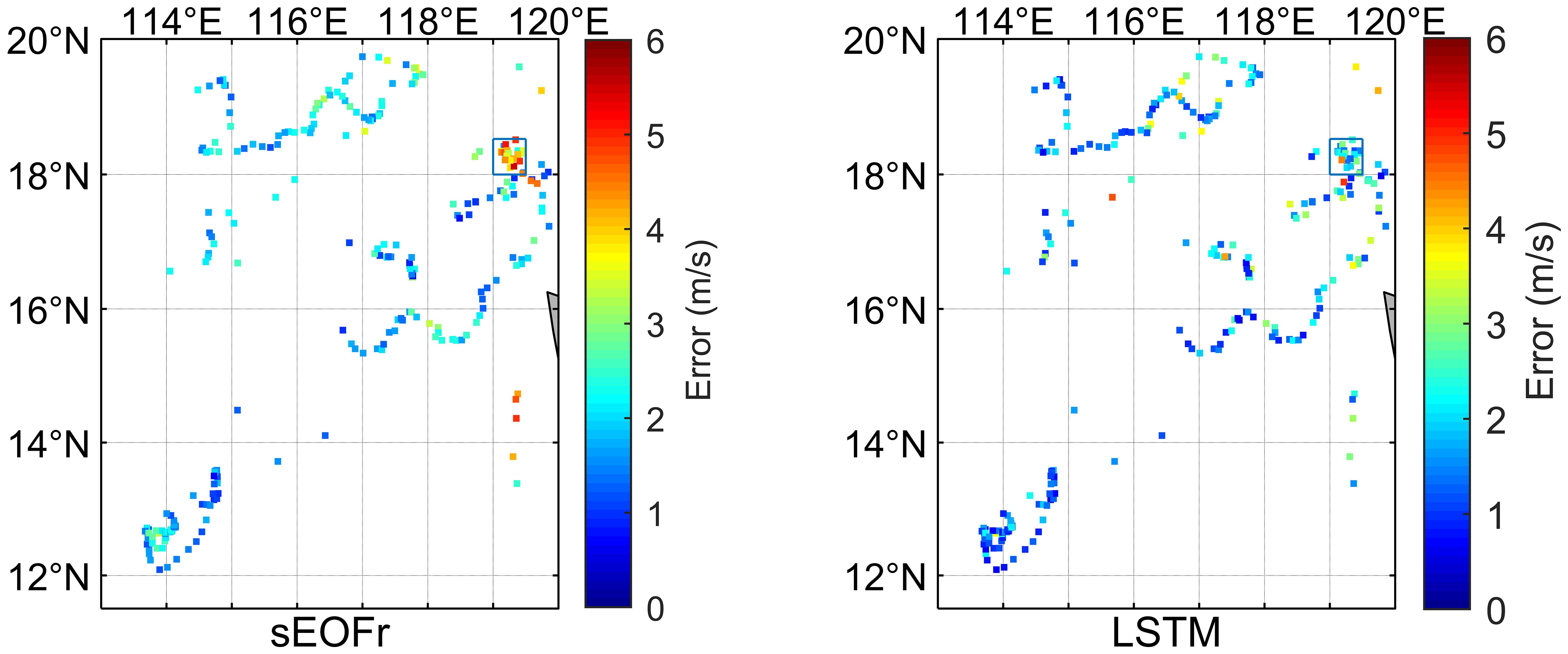
Figure 10 Spatial distribution of the error incurred in the inversion of the SSP.

Figure 11

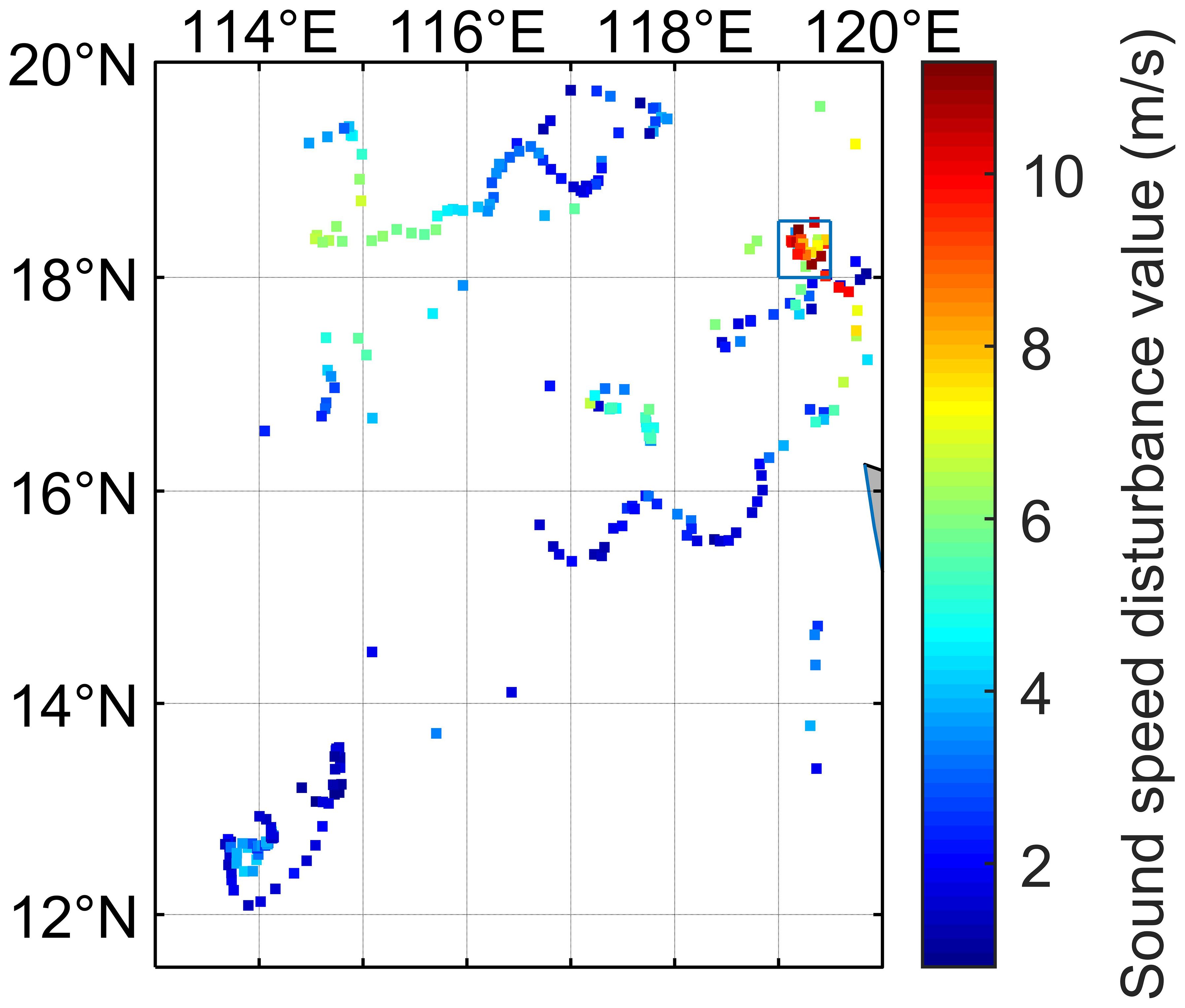
Figure 11 Spatial distribution of the values of disturbance in the sound speed.

4.2 Analysis of area of error concentration

We further investigated the relationship between the RMSE of the reconstructed profile and the values of disturbance in the profile obtained by the Argo data, as shown in Figure 12.

Figure 12

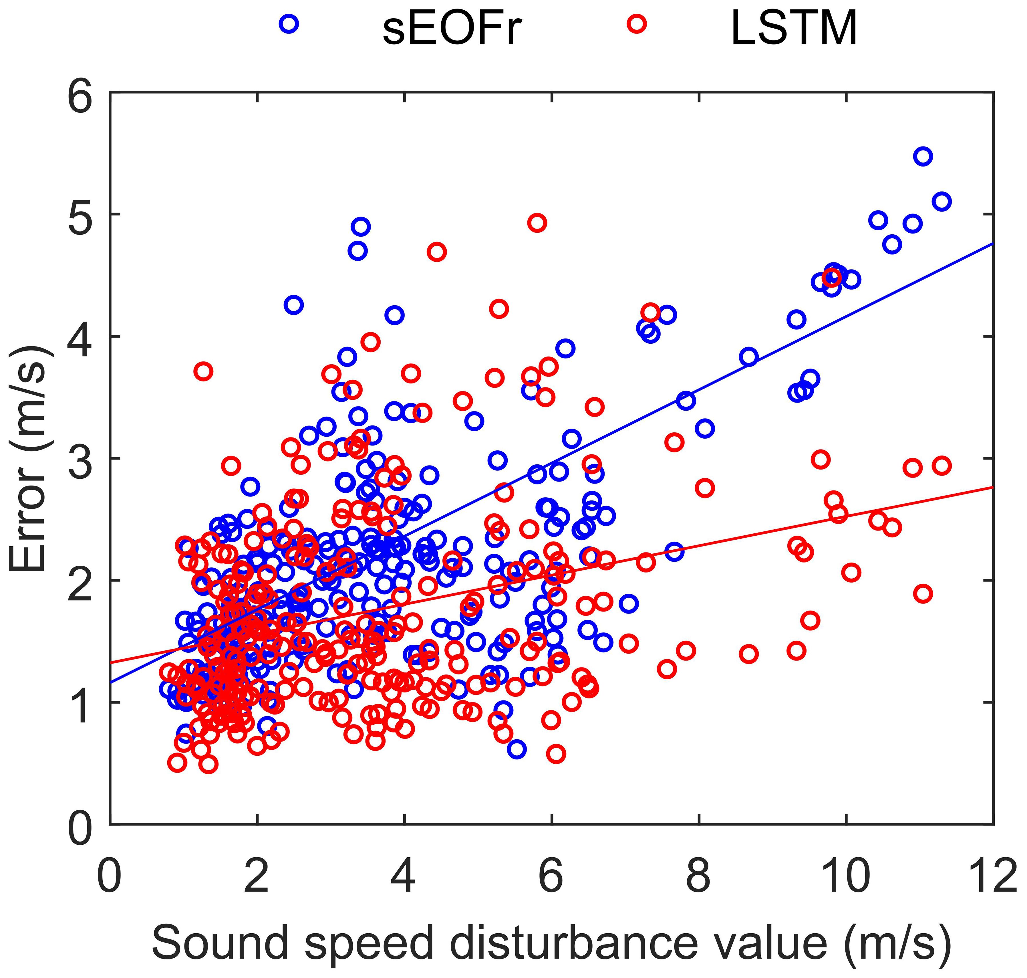
Figure 12 Relationship between Argo profile data reconstruction error and disturbance value.

$\begin{array}{ll}{\text{SSP}}_{\text{sEOFr}}^{\text{rmse}}=0.30\times {\text{SSP}}_{\text{Argo SSP}}^{\text{disturbance}}+1.161& (8)\end{array}$

$\begin{array}{ll}{\text{SSP}}_{\text{LSTM}}^{\text{rmse}}=0.12\times {\text{SSP}}_{\text{Argo SSP}}^{\text{disturbance}}+1.323& (9)\end{array}$

The blue line in the figure represents the results of fitting of the sEOFr model according to Equation 8. Equation 9 shows the results of fitting of the LSTM model, which are represented by the red line in Figure 12. For a deviation of 1 m/s between the profile of the Argo data and the background profile, the error of the sEOFr model increased by 0.30 m/s while that of the LSTM model increased by only 0.12 m/s. The average speed of disturbance in the concentrated area was 8.49 m/s. When Equation 8 is applied to this average disturbance, the calculated RMSE was 3.71 m/s, which is smaller than the actual value of 3.83 m/s. When this average disturbance is substituted into Equation 9, the RMSE was 2.34 m/s, which is greater than the actual error of 2.16 m/s.

The sEOFr model exhibited an advantage over the LSTM model when the disturbance was minor. This is because it is based on a statistical relationship derived from a large amount of historical data. Conversely, the LSTM model delivered superior performance when handling profiles featuring substantial disturbances, with an accuracy that was 43.6% higher on average. Furthermore, the greater the disturbance was (in areas where oceanic activity was frequent and disturbances were substantial) the better was the performance of the LSTM model.

4.3 Validity of results of inversion of acoustic field

The proposed LSTM method guarantees a high accuracy of reconstruction of the SSP, but may not explicitly reveal certain errors in the fine structure of its results. The primary goal of reconstructing the SSP is to calculate the acoustic field, which enables the observation of the fine structure of the SSP. It is important to predict acoustic fields in sonar systems so that targets can be accurately detected. In this section, we report the use of Kraken software to calculate the loss of acoustic transmission in the profile reconstructed by the LSTM model (Model Kraken software is referenced from http://oalib.hlsresearch.com/AcousticsToolbox/), with a significant improvement in the accuracy of reconstruction. The structure of these profiles is illustrated in Figure 13A. Given that the inversion results of the models are only valid within 1000 meters, and the sound speed disturbances below 1000 meters are relatively small, the difference in inversion errors between the two models is not significant. We utilized WOA18 data to fit the sound speed distribution in waters deeper than 1000 meters using empirical formulas. The sound source was 80 m deep, the receiver depth is 80 m with a frequency of 100 Hz, a density of seafloor of 1.5 g/cm3, the seabed sound speed is 1550 m/s, an attenuation coefficient of 0.15 dB/λ, and a depth of water of 3500 m. Figure 13B displays the transmission loss calculated by using the SSPs obtained under these conditions. The sEOFr model recorded an RMSE of 3.83 dB in its calculation of the non-coincident loss of transmission, with 90% of the points yielding errors of 7.75 dB or smaller. The RMSE of the LSTM model was 1.68 dB, with 90% of the points yielding errors of 3.65 dB or smaller. The loss of transmission of both models peaked at 5.5 km, but the loss incurred by the sEOFr model was different by 14.58 dB from the Argo profile, while the LSTM model yielded a difference of only 6.24 dB from it by comparison. After 15 km, the transmission loss calculated by the sEOFr method exhibited a prominent shift in the structure of interference, while the interference structure of LSTM method is basically consistent with Argo. This suggests that the results of inversion of the LSTM model accurately described actual changes in the transmission loss. In most cases, its error was consistently below 3.65 dB.

Figure 13

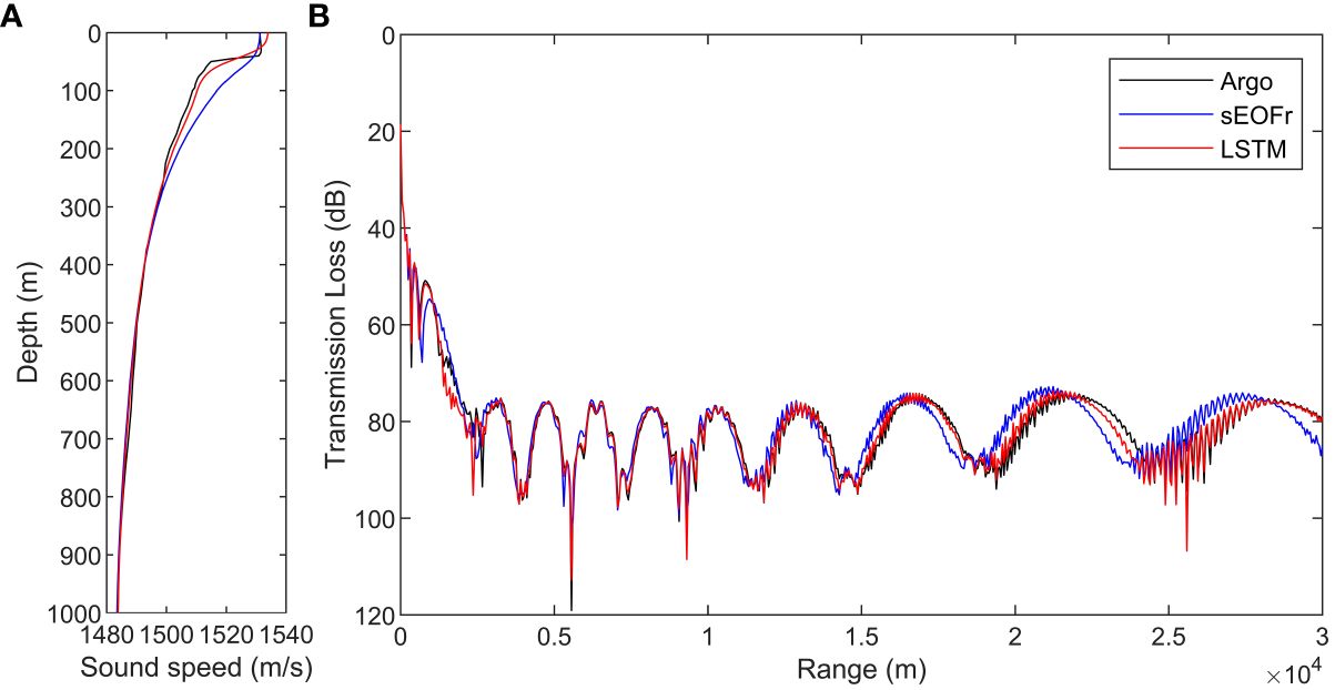
Figure 13 (A, B) Analysis of transmission loss calculated by using the sound speed profile.

Table 1 summarizes the reconstruction results of the two models. The sEOFr model used 3,620 samples to train the model. LSTM trains the model using only 268 samples, of which 8 are the number of samples trained at one time. LSTM model can reconstruct SSP with fewer samples, and its reconstructed RMSE is 1.76m/s, which is more accurate than sEOFr model. In the disturbed area, the accuracy of sEOFr decreases significantly, while the accuracy of LSTM model decreases only a little. The error of sEOFr model is more than twice that of LSTM in predicting propagation loss, and the absolute error range is also twice that of LSTM. Compared with sEOFr model, LSTM model can better solve the problem of sparse sample, large disturbance in sea area, and forecast transmission loss.

Table 1

Table 1 Comparison of inversion results of the two models.

5 Conclusions

In this paper, we proposed a method of SSP inversion based on the LSTM network. By using the parameters of remote sensing as inputs to the model, this method can be used to derive the coefficients of disturbance for SSP inversion. We tested the proposed method on data from the South China Sea and compared its performance with that of the sEOFr model. The results revealed that it had a higher accuracy of inversion of the SSP. It recorded an RMSE that was smaller than that of the sEOFr model by 0.57 m/s, with a 24.46% improvement in accuracy. The concentration of disturbances complicates inversion and reduces the accuracy of the model. However, the memory structure of the proposed LSTM model enabled it to perform well in areas with concentrated disturbances in the sound speed. Furthermore, it delivered excellent performance when the disturbances were large. It reduced the RMSE by 1.67 m/s for such areas in comparison with the sEOFr model, resulting in a 43.60% higher accuracy. This demonstrated its superior performance and robustness in regions with a high concentration of disturbances.

The acoustic field for the profile with the highest improvement in accuracy in inversion based on the LSTM model was calculated by using Kraken software. Its RMSE for the non-coincident loss of transmission was 1.68 dB, with 90% of the error points falling below 3.65 dB. This constituted an improvement of greater than 50% over the sEOFr model, and shows that the proposed LSTM method of SSP inversion can accurately predict changes in the TL.

The proposed non-linear method of SSP inversion is better suited to non-linear relationships between the parameters of the ocean, and yields more accurate outcomes for areas in which traditional models struggle to address concentrated disturbances. The transmission loss in the SSP derived from its approach to inversion more closely approximates the actual profile. This method is important for quickly obtaining the underwater sound field, where this is important for predicting the acoustic field for target detection in sonar systems and underwater acoustic communication.

Data availability statement

The raw data supporting the conclusions of this article will be made available by the authors, without undue reservation.

Author contributions

YZ: Writing – review & editing, Funding acquisition, Project administration, Resources, Validation. PX: Formal analysis, Resources, Supervision, Writing – review & editing. GL: Investigation, Validation, Visualization, Writing – original draft. ZO: Data curation, Project administration, Software, Writing – original draft. KQ: Conceptualization, Funding acquisition, Methodology, Writing – review & editing.

Funding

The author(s) declare financial support was received for the research, authorship, and/or publication of this article. This research was funded by the Natural Science Foundation of Guangdong Province under contract No. 2022A151501151.

Conflict of interest

The authors declare that the research was conducted in the absence of any commercial or financial relationships that could be construed as a potential conflict of interest.

Publisher’s note

All claims expressed in this article are solely those of the authors and do not necessarily represent those of their affiliated organizations, or those of the publisher, the editors and the reviewers. Any product that may be evaluated in this article, or claim that may be made by its manufacturer, is not guaranteed or endorsed by the publisher.

References

Carnes M. R., Mitchell J. L., De Witt P. W. (1990). Synthetic temperature profiles derived from geosat altimetry: comparison with air-dropped expendable bathythermograph profiles. J. Geophys. Res. 95, 17979–17992. doi: 10.1029/JC095iC10p17979

CrossRef Full Text | Google Scholar

Carnes M. R., Teague W. J., Mitchell J. L. (1994). Inference of subsurface thermohaline structure from fields measurable by satellite. J. Atmos. Oceanic Technol. 11, 551–566. doi: 10.1175/1520–0426(1994)011<0551:IOSTSF>2.0.CO;2

CrossRef Full Text | Google Scholar

Chen C., Ma Y., Liu Y. (2018). Reconstructing sound speed profiles worldwide with sea surface data. Appl. Ocean Res. 77, 26–33. doi: 10.1016/j.apor.2018.05.002

CrossRef Full Text | Google Scholar

Del Grosso V. A. (1974). New equation for the speed of sound in natural waters (with comparisons to other equations). J. Acoust. Soc Am. 56, 1084–1091. doi: 10.1121/1.1903388

CrossRef Full Text | Google Scholar

Hochreiter S., Schmidhuber J. (1997). Long short-term memory. Neural. Comput. 9, 1735–1780. doi: 10.1162/neco.1997.9.8.1735

PubMed Abstract | CrossRef Full Text | Google Scholar

Hu J., Kawamura H., Hong H., Qi Y. (2000). A review on the currents in the south China sea: seasonal circulation, south China sea warm current and kuroshio intrusion. J. Oceanogr. 56, 607–624. doi: 10.1023/A:1011117531252

CrossRef Full Text | Google Scholar

Jain S., Ali M. M. (2006). Estimation of sound speed profiles using artificial neural networks. IEEE Geosci. Remote Sens. Lett. 3, 467–470. doi: 10.1109/LGRS.2006.876221

CrossRef Full Text | Google Scholar

Jain G., Sharma M., Agarwal B. (2019). Optimizing semantic LSTM for spam detection. Int. J. Inf. Tecnol. 11, 239–250. doi: 10.1007/s41870-018-0157-5

CrossRef Full Text | Google Scholar

Khataei Maragheh H., Gharehchopogh F.S. Majidzadeh K., Sangar A. B. (2022). A new hybrid based on long short-term memory network with spotted hyena optimization algorithm for multi-label text classification. . Math 10, 488. doi: 10.3390/math10030488

CrossRef Full Text | Google Scholar

Klemas V., Yan X.-H. (2014). Subsurface and deeper ocean remote sensing from satellites: an overview and new results. Prog. Oceanogr. 122, 1–9. doi: 10.1016/j.pocean.2013.11.010

CrossRef Full Text | Google Scholar

LeBlanc L. R., Middleton F. H. (1980). An underwater acoustic sound velocity data model. J. Acoust. Soc. Am. 67, 2055–2062. doi: 10.1121/1.384448

CrossRef Full Text | Google Scholar

Li Y., Gao P., Tang B., Yi Y., Zhang J. (2022a). Double feature extraction method of ship-radiated noise signal based on slope entropy and permutation entropy. Entropy 24, 22. doi: 10.3390/e24010022

CrossRef Full Text | Google Scholar

Li Y., Geng B., Jiao S. (2022b). Dispersion entropy-based lempel-ziv complexity: A new metric for signal analysis. Chaos Solitons Fractals 161, 112400. doi: 10.1016/j.chaos.2022.112400

CrossRef Full Text | Google Scholar

Li H., Qu K., Zhou J. (2021). Reconstructing sound speed profile from remote sensing data: nonlinear inversion based on self-organizing map. IEEE Access 9, 109754–109762. doi: 10.1109/ACCESS.2021.3102608

CrossRef Full Text | Google Scholar

Li Y., Tang B., Yi Y. (2022c). A novel complexity-based mode feature representation for feature extraction of ship-radiated noise using VMD and slope entropy. Appl. Acoustics 196, 108899. doi: 10.1016/j.apacoust.2022.108899

CrossRef Full Text | Google Scholar

Liu Y., Chen W., Chen Y., Chen W., Ma L., Meng Z. (2021). Ocean front reconstruction method based on K-means algorithm iterative hierarchical clustering sound speed profile. JMSE 9, 1233. doi: 10.3390/jmse9111233

CrossRef Full Text | Google Scholar

Liu L., Silver D., Bemis K. (2021). Visualizing acoustic imaging of hydrothermal plumes on the seafloor. IEEE Comput. Grap. Appl. 41, 63–75. doi: 10.1109/MCG.2020.2995077

CrossRef Full Text | Google Scholar

Luo P., Song Y., Xu X., Wang C., Zhang S., Shu Y., et al. (2022). Efficient underwater sensor data recovery method for real-time communication subsurface mooring system. JMSE 10, 1491. doi: 10.3390/jmse10101491

CrossRef Full Text | Google Scholar

Ou Z., Qu K., Shi M., Wang Y., Zhou J. (2022). Estimation of sound speed profiles based on remote sensing parameters using a scalable end-to-end tree boosting model. Front. Mar. Sci. 9. doi: 10.3389/fmars.2022.1051820

PubMed Abstract | CrossRef Full Text | Google Scholar

Rahaman H., Behringer D. W., Penny S. G., Ravichandran M. (2016). Impact of an upgraded model in the NCEP global ocean data assimilation system: the tropical Indian ocean: NCEP-GODAS ANALYSIS WITH MOM4P1. J. Geophys. Res. Oceans 121, 8039–8062. doi: 10.1002/jgrc.v121.11

CrossRef Full Text | Google Scholar

Stammer D. (1997). Global characteristics of ocean variability estimated from regional TOPEX/POSEIDON altimeter measurements. J. Phys. Oceanogr. 27, 1743–1769. doi: 10.1175/1520–0485(1997)027<1743:GCOOVE>2.0.CO;2

CrossRef Full Text | Google Scholar

Su J., Li Y., Ali W. (2022). Underwater passive manoeuvring target tracking with isogradient sound speed profile. IET Radar Sonar Navi 16, 1415–1433. doi: 10.1049/rsn2.12269

CrossRef Full Text | Google Scholar

Su H., Wu X., Yan X.-H., Kidwell A. (2015). Estimation of subsurface temperature anomaly in the Indian ocean during recent global surface warming hiatus from satellite measurements: A support vector machine approach. Remote. Sens. Environ. 160, 63–71. doi: 10.1016/j.rse.2015.01.001

CrossRef Full Text | Google Scholar

Su H., Yang X., Lu W., Yan X.-H. (2019). Estimating subsurface thermohaline structure of the global ocean using surface remote sensing observations. Remote Sens. 11, 1598. doi: 10.3390/rs11131598

CrossRef Full Text | Google Scholar

Sun S., Fang Y., Zu Y., Liu B., Tana Samah A. (2020). A seasonal characteristics of mesoscale coupling between the sea surface temperature and wind speed in the south China sea. J. Clim. 33, 625–638. doi: 10.1175/JCLI-D-19-0392.1

CrossRef Full Text | Google Scholar

Teymorian A. Y., Cheng W., Ma L., Cheng X., Lu X., Lu Z. (2009). 3D underwater sensor network localization. IEEE Trans. Mobile Comput. 8, 1610–1621. doi: 10.1109/TMC.2009.80

CrossRef Full Text | Google Scholar

Wang R., Peng C. Gao J., Gao Z., Jiang H. (2020). A dilated convolution network-based LSTM model for multi-step prediction of chaotic time series. Comp. Appl. Math. 39, 30. doi: 10.1007/s40314-019-1006-2

CrossRef Full Text | Google Scholar

Wunsch C. (1997). The vertical partition of oceanic horizontal kinetic energy. J. Phys. Oceanogr. 27, 1770–1794. doi: 10.1175/1520–0485(1997)027<1770:TVPOOH>2.0.CO;2

CrossRef Full Text | Google Scholar

Xiao J., Xie Q. Liu C., Chen J., Wang D., Chen M. (2013). A diagnostic model of the South China Sea bottom circulation inconsideration of tidal mixing, eddy-induced mixing and topography. Acta Oceanol Sin. (in Chinese) 35, 01–13. doi: 10.3969/j.issn.0253–4193.2013.05.001

CrossRef Full Text | Google Scholar

Xu P., Ando M., Tadokoro K. (2005). Precise, three-dimensional seafloor geodetic deformation measurements using difference techniques. Earth Planet Sp 57, 795–808. doi: 10.1186/BF03351859.\

CrossRef Full Text | Google Scholar

Xu C., Li H., Chen B., Zhou T. (2013). Multibeam interferometric seafloor imaging technology. J. Harbin Eng. 34, 1159–1164. doi: 10.3969/j.issn.1006–7043.201302007

CrossRef Full Text | Google Scholar

Yan K., Wang Y., Xiao W. (2022). A new compression and storage method for high-resolution SSP data based-on dictionary learning. JMSE 10, 1095. doi: 10.3390/jmse10081095

CrossRef Full Text | Google Scholar

Zhan D., Wang S., Cai S., Zheng H., Xu W. (2023). Acoustic localization with multi-layer isogradient sound speed profile using TDOA and FDOA. Front. Inform Technol. Electron Eng. 24, 164–175. doi: 10.1631/FITEE.2100398

CrossRef Full Text | Google Scholar