A transformer-based method for correcting significant wave height numerical forecasting errors

Accurate significant wave height (SWH) forecasting is essential for various marine activities. While traditional numerical and mathematical-statistical methods have made progress, there is still room for improvement. This study introduces a novel transformer-based approach called the 2D-Geoformer to enhance SWH forecasting accuracy. The 2D-Geoformer combines the spatial distribution capturing capabilities of SWH numerical models with the ability of mathematical-statistical methods to identify intrinsic relationships among datasets. Using a comprehensive long time series of SWH numerical hindcast datasets as the numerical forecasting database and ERA5 reanalysis SWH datasets as the observational proxies database, with a focus on a 72-hour forecasting window, the 2D-Geoformer is designed. By training the potential connections between SWH numerical forecasting fields and forecasting errors, we can retrieve SWH forecasting errors for each numerical forecasting case. The corrected forecasting results can be obtained by subtracting the retrieved SWH forecasting errors from the original numerical forecasting fields. During long-term validation periods, this method consistently and effectively corrects numerical forecasting errors for almost every case, resulting in a significant reduction in root mean square error compared to the original numerical forecasting fields. Further analysis reveals that this method is particularly effective for numerical forecasting fields with higher errors compared to those with relatively smaller errors. This integrated approach represents a substantial advancement in SWH forecasting, with the potential to improve the accuracy of operational SWH forecasts. The 2D-Geoformer combines the strengths of numerical models and mathematical-statistical methods, enabling better capture of spatial distributions and intrinsic relationships in the data. The method's effectiveness in correcting numerical forecasting errors, particularly for cases with higher errors, highlights its potential for enhancing SWH forecasting accuracy in operational settings.

1 Introduction

Significant wave height (SWH) constitutes an essential aspect of marine surface dynamics, encapsulating the mean peak of the highest third of waves (Zhang, 2012; Qiu et al., 2019). This metric is of substantial consequence, underpinning safety and operational planning across a broad array of maritime, research, and recreational activities (Qiu et al., 2019). Accurate SWH forecasts are particularly vital for the northwestern Pacific region, where maritime economic activities are bustling, and the presence of tropical cyclones introduces considerable variability, making reliable predictions a complex and challenging task. The accurate prediction of SWH is essential not only for safeguarding maritime navigation but also for advancing scientific knowledge and enhancing oceanic enjoyment. However, achieving precise forecasts is inherently difficult due to the dynamic interplay of various factors that influence wave generation, growth, and dissipation. These factors include a range of kinetic, physical, and environmental conditions, underscoring the substantial scientific endeavor involved in improving SWH prediction accuracy (Zhang et al., 2009; Xiao et al., 2023).

In the realm of SWH forecasting, two predominant methodologies are recognized. The first hinges on physical-dynamic principles, utilizing wave numerical models that meticulously simulate the birth, movement, and fading of ocean waves through the computational resolution of the underlying wave dynamic equations. These models incorporate a suite of physical processes such as wave generation, spectral distribution, propagation, nonlinear inter-wave interactions, dissipation mechanisms, and the effects of refraction and diffraction (Zhao et al., 2014; Qiao et al., 2016; Bennis et al., 2020; Wang et al., 2021; Bitner-Gregersen et al., 2022; Saavedra et al., 2023). Prominent among such numerical models are the Wave Watch III (WW3) (Tolman, 2009; Amarouche et al., 2023), the Simulating Waves Nearshore (SWAN) system (Booij et al., 1999; Ris et al., 1999), and the MASUM model (Yong-zeng et al., 2005). Each of these has demonstrated exceptional efficacy in predicting SWH, as substantiated by various studies (Wang et al., 2016; Ponce De León et al., 2018; Qiu et al., 2019). Presently, operational wave forecasting systems predominantly rely on these advanced numerical wave models to deliver accurate SWH forecasts.

Alternative methods for forecasting SWH utilize mathematical-statistical approaches. These can be broadly categorized into point forecasting and spatiotemporal forecasting. Point forecasting delves into the spectral features, context, and temporal dependencies within SWH sequences to facilitate continuous time series forecasting. This category encompasses a variety of methods such as wavelet analysis, Particle Swarm Optimization (PSO), Extreme Learning Machine (ELM) approaches, Bayesian hyperparameter optimization, Elastic Net methods, Singular Value Decomposition (SVD), and Empirical Mode Decomposition (EMD) (Altunkaynak, 2015; Kaloop et al., 2020; Pirhooshyaran and Snyder, 2020; Demetriou et al., 2021; Zhou et al., 2021; Çelik, 2022). An expanded version of point forecasting not only analyzes the time evolution of SWH but also integrates influencing factors like wind speed, direction, duration, fetch, sea level pressure, and air temperature. Techniques in this domain include Long Short-Term Memory (LSTM) networks, hierarchical machine learning models, Artificial Neural Networks (ANN), Multiple Additive Regression Trees (MART), hybrid models of wavelets and neural networks (WNN), and Pruning Radial Basis Function (GAP-RBF) networks (Fernández et al., 2015; Kumar et al., 2017; Oh and Suh, 2018; Fan et al., 2020; Elbisy and Elbisy, 2021; Shi et al., 2023).

Spatiotemporal forecasting goes a step further by considering both the time evolution and spatial correlations of SWH, along with the spatiotemporal dynamics of influencing meteorological factors. This approach broadens the forecasting scope to encompass entire regions. Examples of such comprehensive methodologies include convolutional LSTM networks and multivariate 3-layer LSTM-based methods, which offer a more integrated and regionally encompassing forecast of SWH (Han et al., 2022; Song et al., 2022; Zilong et al., 2022). These sophisticated techniques aspire to capture the complexity of wave dynamics across both time and space for enhanced maritime prediction accuracy.

Advancements in mathematical-statistical methodologies have substantially progressed SWH forecasting. However, they have not achieved the predictive accuracy comparable to numerical wave models (Choi et al., 2020; Zhang et al., 2021). This gap is attributed to the reliance of traditional approaches on long-term observational data, which often overlooks the advancements in numerical wave modeling that significantly enhance SWH forecasting. While numerical models offer improved accuracy, their performance is dependent on the quality of input data, model resolution, and precise representation of physical processes. Any inaccuracies in these factors can critically affect forecast outcomes (Wang et al., 2016; Ponce De León et al., 2018; Allahdadi et al., 2019; Amarouche et al., 2023; Xiao et al., 2023).

Despite these shortcomings, mathematical-statistical methods excel in uncovering complex correlations within datasets, while numerical models proficiently capture the physical dynamics of SWH. Acknowledging these strengths and limitations, our study proposes a novel integrated approach that merges the precision of numerical wave models with the analytical capabilities of mathematical-statistical methods. This synergy aims to harness the high predictive accuracy of numerical models and the deep analytical insights of statistical approaches.

At the heart of our methodology is the deployment of transformer techniques, renowned for their proficiency in data analysis, particularly within the context of Spatiotemporal Attention Mechanisms. These mechanisms enable the model to dynamically focus on relevant spatial and temporal features, enhancing its ability to understand complex patterns and relationships in the data. By leveraging these advanced transformer methods, our approach not only captures the intricate dynamics of spatiotemporal data but also significantly improves the accuracy and efficiency of predictions across various applications. This integration of spatiotemporal attention with transformer architectures represents a substantial advancement in the field, offering a powerful tool for analyzing and forecasting data that varies both across space and over time (Zheng et al., 2021; Zhou and Zhang, 2023; Bertasius et al., 2021; Vaswani et al., 2017). These methods are applied to historical hindcast SWH datasets to scrutinize and characterize the evolution of forecasting errors. Our primary aim is to develop an advanced diagnosing model that rectifies inherent errors in numerical predictions. This strategy seeks to amalgamate two distinct forecasting methodologies, providing a more accurate and holistic tool for SWH prediction. Through this integration, our goal is to significantly enhance SWH forecasting, thereby contributing to the safety and efficiency of maritime operations.

2 Data and methodology

2.1 Data

The SWH hindcast data employed in this study is sourced from an ocean forecasting system specifically tailored for the 21st-Century Maritime Silk Road (Qiao et al., 2019). This system is based on the surface wave-tide-circulation coupled ocean model developed by the First Institute of Oceanography (FIO-COM), Ministry of Natural Resources, China. It was officially commenced operational service on Dec. 10, 2018, and represents a significant milestone in Chinese oceanographic modeling. The dataset spanning from its inception date Dec. 10, 2018, to Nov. 29, 2023, forms the basis of the analysis presented in this research. The hindcast process within this system is executed daily at 12:00 UTC, ensuring a consistent and continuous flow of data. Although the model is capable of global coverage, to optimize computational efficiency and resource management, our study has strategically focused on the northwestern Pacific region, defined by the coordinates 98°E to 175°E and 18°S to 48°N. This particular area is not only of crucial importance to the Maritime Silk Road initiative but also presents a diverse range of oceanographic and meteorological conditions, making it an ideal subject for detailed study. To capture the dynamic nature of the ocean environment, the model operates with a high spatio-temporal resolution. Data is updated every three hours, and the spatial resolution is set at 0.1° by 0.1°. This level of detail in the model’s output allows for an in-depth analysis of wave patterns, providing valuable insights into the marine conditions along one of the world’s most vital maritime routes. The utilization of this data is pivotal in enhancing our understanding of the oceanic conditions along the Maritime Silk Road. This, in turn, informs safer and more efficient maritime navigation, aids in the design of maritime structures, and supports climatological research relevant to the region.

The gridded SWH reanalysis data from ERA5, developed by the European Centre for Medium-Range Weather Forecasting (ECMWF), is utilized in this research. As a global reanalysis dataset, ERA5 marks a substantial progression in atmospheric analysis, incorporating advanced methodologies to aggregate diverse meteorological data (Hersbach et al., 2020). The SWH reanalysis datasets were generated by applying ERA5 wind fields to drive the Wave Model (WAM) with Source Term 3 (ST3) physics (Group, 1988), supplemented by the assimilation of extensive altimeter data (Lionello et al., 1992). We procured ERA5 SWH data on a 0.25° by 0.25° grid, covering the period from Dec. 10, 2018, to Dec 2, 2023, focusing on the area between 98°E to 175°E and 18°S to 48°N, with data updated every 3 hours. The precision of the ERA5 dataset in depicting actual SWH characteristics is exceptional, establishing it as a crucial instrument for wave analysis (Shi et al., 2021; Wang and Wang, 2022). Due to its accuracy, it is increasingly used as an alternative to traditional grid observations of SWH (Muhammed Naseef and Sanil Kumar, 2020; Takbash and Young, 2020). In this paper, the ERA5 SWH data is employed to correct forecasting errors in the numerical SWH predictions made by the FIO-COM.

Our study is dedicated to examining the distribution and temporal evolution of errors in SWH forecasting, and their interrelationship with the distribution and evolution of forecasted SWH. Following this analysis, we propose to develop a deep learning model specialized in diagnosing these errors, utilizing the forecasted SWH as a foundational dataset. In an effort to balance computational efficiency with the need for reliable data, we have opted for a grid resolution of 0.5° by 0.5°. This choice allows us to manage the vast data effectively while maintaining sufficient detail for accurate analysis. Both the SWH forecasting results and the ERA5 reanalysis data have been meticulously interpolated to this standardized grid, ensuring consistency in our spatial analysis. Our focus is narrowed to short-term forecasting, specifically targeting a 72-hour period with intervals of 3 hours. This temporal restriction enables us to effectively manage and reduce the dimensionality of our dataset to ${\text{N}}_{\text{time}}\times {\text{N}}_{\text{lat}}\times {\text{N}}_{\text{lon}}=25\times 132\times 154$, making the data more tractable for extensive computational processing. The forecasting errors for each hindcast scenario is performed by deducting the ERA5 reanalyzed SWH values from the forecasted SWH fields. The resulting processed SWH forecasting fields, alongside the error fields, constitute an extensive database for the training and validation of our deep learning model, laying a robust groundwork for enhancing the accuracy and reliability of SWH forecasting.

2.2 Methodology

2.2.1 2D-Geoformer methods

In this study, we have employed a model that is a customized adaptation of Zhou’s 3D-Geoformer (Zhou and Zhang, 2023), specifically modified for our two-dimensional (2D) case studies and thus aptly named the 2D-Geoformer. While the original 3D-Geoformer by Zhou is developed for analyzing three-dimensional multivariate distributions and their spatiotemporal interactions, our adaptation, the 2D-Geoformer, focuses on the horizontal spatiotemporal attention aspects pertinent to SWH forecasting and its associated errors. This adaptation takes into account the crucial relationship between the forecasted SWH and its corresponding errors. In alignment with the architecture of leading transduction models, the 2D-Geoformer is constructed on an encoder-decoder framework, encompassing various integral components. These include two data preprocessing modules designed to optimally prepare the input data, the encoder and decoder units that are central to the model’s processing and predictive capabilities, and an output layer that synthesizes and outputs the model’s predictions. The detailed architecture and functionality of these components are comprehensively documented in the Appendix.

The 2D-Geoformer model processes 25 sets of forecast data as inputs (${\text{X}}_{{\text{T}}_{\text{in}}\times {\text{N}}_{\text{lat}}\times {\text{N}}_{\text{lon}}}^{\text{in}}$), each representing SWH predictions every 3 hours over a 72-hour period. The data’s dimensions are ${\text{T}}_{\text{in}}\times {\text{N}}_{\text{lat}}\times {\text{N}}_{\text{lon}}=25\times 132\times 154$, where ${\text{N}}_{\text{lat}}\times {\text{N}}_{\text{lon}}$denotes the spatial grid points. The model aims to diagnose the following 25 sets of forecasting error fields with the same dimension (${\text{X}}_{{\text{T}}_{\text{out}}\times {\text{N}}_{\text{lat}}\times {\text{N}}_{\text{lon}}}^{\text{out}}$). As illustrated in Figure 1A, the preprocessing module initially handles the inputs ${\text{X}}_{{\text{T}}_{\text{in}}\times {\text{N}}_{\text{lat}}\times {\text{N}}_{\text{lon}}}^{\text{in}}$by dividing them into non-overlapping patches of size $h_0\times w_0=4\times 4$ across the channel dimension. These patches are transformed into symbolic representations with embedded spatiotemporal data (Figure 1B). The symbolic representations are then processed by the encoder, consisting of four identical encoding blocks $n=4$. Each encoding block includes a multi-headed spatiotemporal attention layer (with eight heads, as shown in Figure 1C) and a fully connected network. This encoder compresses the representations into a feature map matrix for the 25 inputs. Subsequently, this feature map is analyzed by the decoder through four decoding blocks ($m=4$). Finally, the model outputs are mapped to forecast error fields. ${\text{X}}_{{\text{T}}_{\text{out}}\times {\text{N}}_{\text{lat}}\times {\text{N}}_{\text{lon}}}^{\text{out}}$, maintaining the same spatial resolution as the input SWH forecasting fields in the output layer.

Figure 1

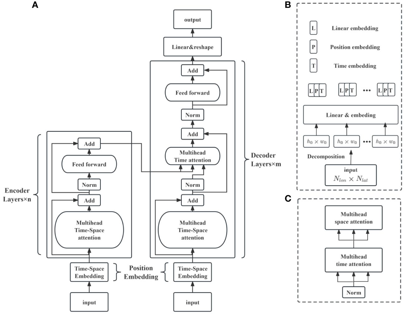
Figure 1 Schematic Overview of the 2D-Geoformer Model for SWH forecasting Error retrieving. (A) Depicts the comprehensive architecture of the 2D-Geoformer, which includes dual preprocessing modules at the bases of the encoder and decoder stacks, an advanced encoder-decoder framework utilizing a multiheaded spatiotemporal attention mechanism, and a final output layer concluding the decoder. The input to the model comprises 25 time steps of SWH forecasts, with each step representing a 3-hour interval; these are paired with corresponding SWH forecasting error fields at identical forecast hours, serving as target retrieving fields for supervised training. (B) Details the intricate design of the preprocessing module, which encompasses a field decomposition and a patch embedding process. (C) Illustrates the complex structure of the multihead spatiotemporal attention module.

2.2.2 Model training strategy

The 2D-Geoformer model employs SWH forecasts as inputs and targets the corresponding 25 forecasting errors as output fields, leveraging self-attention mechanisms for efficient model training. This method significantly mitigates error growth typically seen in sliding prediction strategies. To evaluate the relationship between retrieved and actual errors, we adopt the root mean square error (RMSE) as our loss function, which quantifies the deviation between retrieved and actual errors. The loss function is defined as:

$$\text{Loss}=\frac{1}{{\text{T}}_{\text{out}}}\sum _{\text{t}=1}^{{\text{T}}_{\text{out}}}\sqrt{\frac{1}{{\text{N}}_{\text{lat}}\times {\text{N}}_{\text{lon}}}{\displaystyle \sum _{\text{i}=1}^{{\text{N}}_{\text{lon}}}}{\displaystyle \sum _{\text{j}=1}^{{\text{N}}_{\text{lat}}}}{({\text{X}}_{\text{t}.\text{j}.\text{i}}^{\text{out}}-{\text{X}}_{\text{t}.\text{j}.\text{i}}^{\text{tg}})}^2}$$

Here, $X^{tg}$ represents the actual error fields of FIO-COM forecasts, and $X^{out}$ denotes the output fields retrieved from the 2D-Geoformer.

For optimization, we employ the Adam algorithm, enhanced with a learning rate warm-up strategy starting at an initial rate of $1\times {10}^{-4}$. Post each training epoch, we assess the model’s RMSE accuracy using the validation set and retain the model parameters that yield the least RMSE.

We have utilized hindcast datasets spanning from Dec. 10, 2018, to Dec. 31, 2022, for training, and datasets from Jan. 01, 2023, to Nov. 29, 2023, for testing. It is important to note that our dataset’s spatial domain includes land regions, which can significantly interfere with error correction. To minimize this impact, we implemented a strategy of nullifying data from these land areas. This approach ensures that the model predominantly focuses on marine regions, thereby more precisely capturing the spatiotemporal distribution of SWH and improving the correction model’s effectiveness.

3 Results

3.1 The overall correction effects

In the correction phase, each numerical forecast instance employs SWH forecasts generated by FIO-COM, featuring predictions at 3-hour intervals across a 72-hour timeframe, as input for the 2D-Geoformer model. This model subsequently identifies potential errors within the FIO-COM SWH predictions. The identified errors are regarded as estimated discrepancies for the FIO-COM SWH forecasts. These estimated errors are then deducted from the FIO-COM predictions to produce the adjusted SWH forecasts.

Following this correction procedure, an error statistical analysis is conducted, comparing the original FIO-COM SWH forecasts and the corrected SWH forecasts against reanalysis SWH datasets, which serve as observational benchmarks. This validation process is systematically repeated for each hindcast forecast case spanning from Jan. 01, 2023, to Nov. 29, 2023. While error correction is performed across all 25 time steps within the 72-hour forecasting period, our analysis primarily focuses on samples at 24, 48, and 72-hour forecast intervals. The reason for this targeted analysis is that the correction effects observed at these specific intervals (24H, 48H, 72H) are representative of the overall performance across all time steps. This approach ensures a comprehensive understanding of the model’s correction efficacy at critical forecasting junctures, thereby providing a robust evaluation of the 2D-Geoformer’s capabilities in enhancing SWH forecast accuracy.

Following correction, the SWH forecasting accuracy of FIO-COM demonstrates significant enhancement, a phenomenon consistently observed across various cases within the evaluation period. As illustrated in Figure 2A, the spatially-averaged RMSE values for the adjusted SWH forecasts are substantially lower than those of the original FIO-COM forecasts for the selected intervals. To quantify this enhancement, the differential in RMSE between the original and corrected SWH forecasts is calculated. Figure 2B presents this comparison, indicating that the correction process decreases the RMSE by a range of 0.0 to 0.37, thereby highlighting the efficacy of the correction methodology. It is noteworthy that a marginal decline in correction effectiveness becomes apparent as the forecast horizon extends, reflecting the expected escalation in complexity and uncertainty associated with error evolution over more extended forecasting periods.

Figure 2

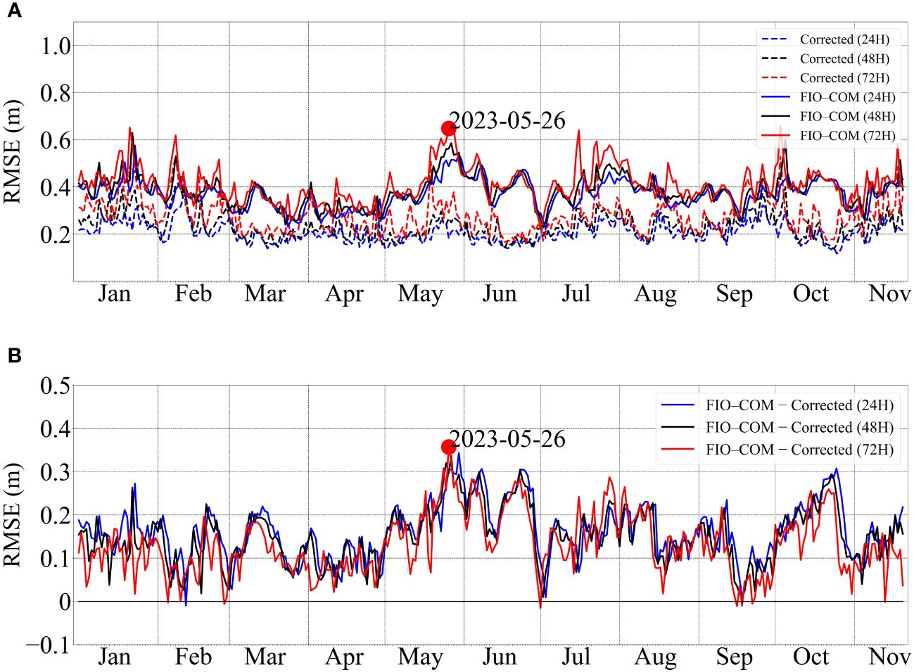
Figure 2 (A) Time series of spatial-averaged RMSE (Units: m) for forecasting intervals at 24, 48, and 72 hours, comparing between original SWH forecasts of FIO-COM and the corrected fields in 2023. (B) Illustrates the differential analysis of RMSE skills between the original FIO-COM and corrected SWH forecasts. A specific dotted hindcast scenario, initiated on May. 26, 2023, at 12:00 UTC, is marked for detailed case analysis.

This comprehensive analysis of RMSE values, covering all cases throughout the testing period, offers deeper insights into the efficacy of the correction methodology applied to the FIO-COM SWH forecasts (Table 1). Initially, the uncorrected FIO-COM model demonstrated average RMSEs of 0.37, 0.38, and 0.41 for forecast intervals of 24, 48, and 72 hours, respectively. Post-correction, these RMSE values showed a significant reduction, dropping to 0.21, 0.23, and 0.28, respectively. This substantial reduction in RMSE indicates not only an enhancement in forecast accuracy but also the uniform effectiveness of the correction method across various forecasting horizons. In quantitative terms, this improvement translates to overall accuracy enhancements of 43.2%, 39.5%, and 31.7% for each respective interval. Such a marked advancement in forecast precision, underscores the robustness and efficiency of the adopted correction methodology. Intriguingly, as forecasting intervals extend, a marginal increase in RMSE for both pre- and post-correction forecasts was observed, indicating a diminishing impact of both the numerical model and correction methods over prolonged forecasting periods. This trend highlights the increasing complexity and nuanced challenges in long-term forecasting. Additionally, the diminishing percentage of improvement with extended forecasting intervals suggests a gradual reduction in the correction method’s effectiveness in longer-term forecasts, further emphasizing the need for refined approaches in extended forecasting scenarios.

Table 1

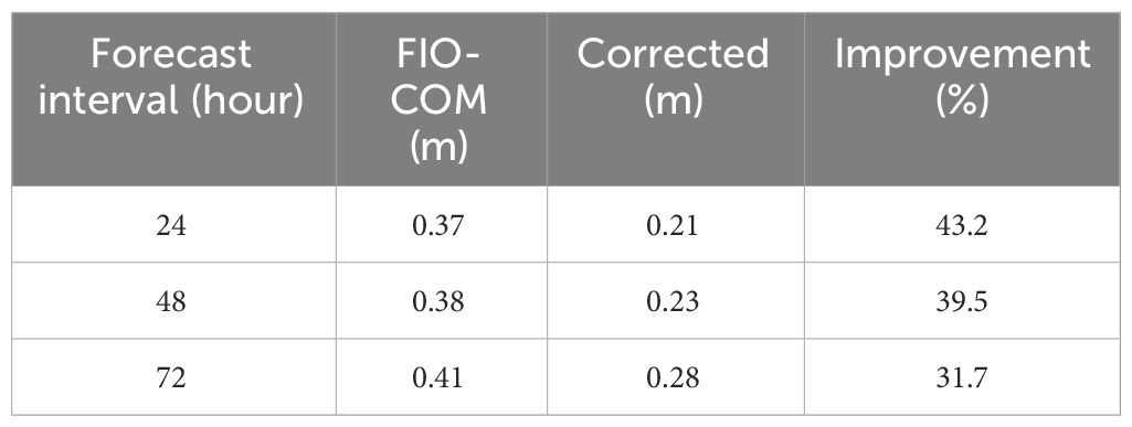
Table 1 Average RMSE comparisons for all testing cases between FIO-COM and the corrected forecasts, along with the percentage improvement post-correction at 24, 48, and 72 forecasting hours.

Such a significant enhancement in forecast accuracy is particularly remarkable, given the advanced state of current SWH numerical models. The fact that substantial improvements are achieved not through fundamental optimizations in the numerical model but rather through post-processing corrections is a testament to the innovative approach and effectiveness of the 2D-Geoformer model. This outcome highlights the potential of integrating advanced data correction techniques in enhancing the accuracy of established numerical wave prediction models.

The preceding analysis yields a comprehensive understanding of the overall correction effects on the FIO-COM model’s forecasts. However, it primarily provides a macroscopic perspective, lacking in detailed spatial distribution insights of these correction effects. To address this gap, a granular investigation was conducted on the RMSE values at each grid point across the 24, 48, and 72-hour forecast intervals during the entire testing period. This approach facilitates a more nuanced understanding of the spatial variability in the correction effectiveness. By analyzing the RMSE at each grid point, we can discern specific areas where the correction methodology had pronounced impacts, as well as regions where it was less effective. Such spatially-resolved analysis not only enhances the depth of our understanding but also provides critical insights that can guide future improvements in the correction process and its application in varying geographic contexts.

Figures 3A–C depict an upward trend in the RMSE for the FIO-COM model as the forecasting interval extends from 24 to 72 hours. Notably, RMSE values are higher in the northern and southeastern sectors of the study area, often exceeding 0.4 meters, which suggests a lower predictive accuracy in these regions. Conversely, the southwestern sector demonstrates stronger model performance, with RMSE values typically below 0.3 meters. After correction, there is a significant reduction in RMSE across all forecasting periods (Figures 3D–F, G–I), especially in the southeastern area where the RMSE decreases from above 0.4 meters to below 0.3 meters. Although the reduction in the northeastern section is less pronounced, the improvement in RMSE is still significant.

Figure 3

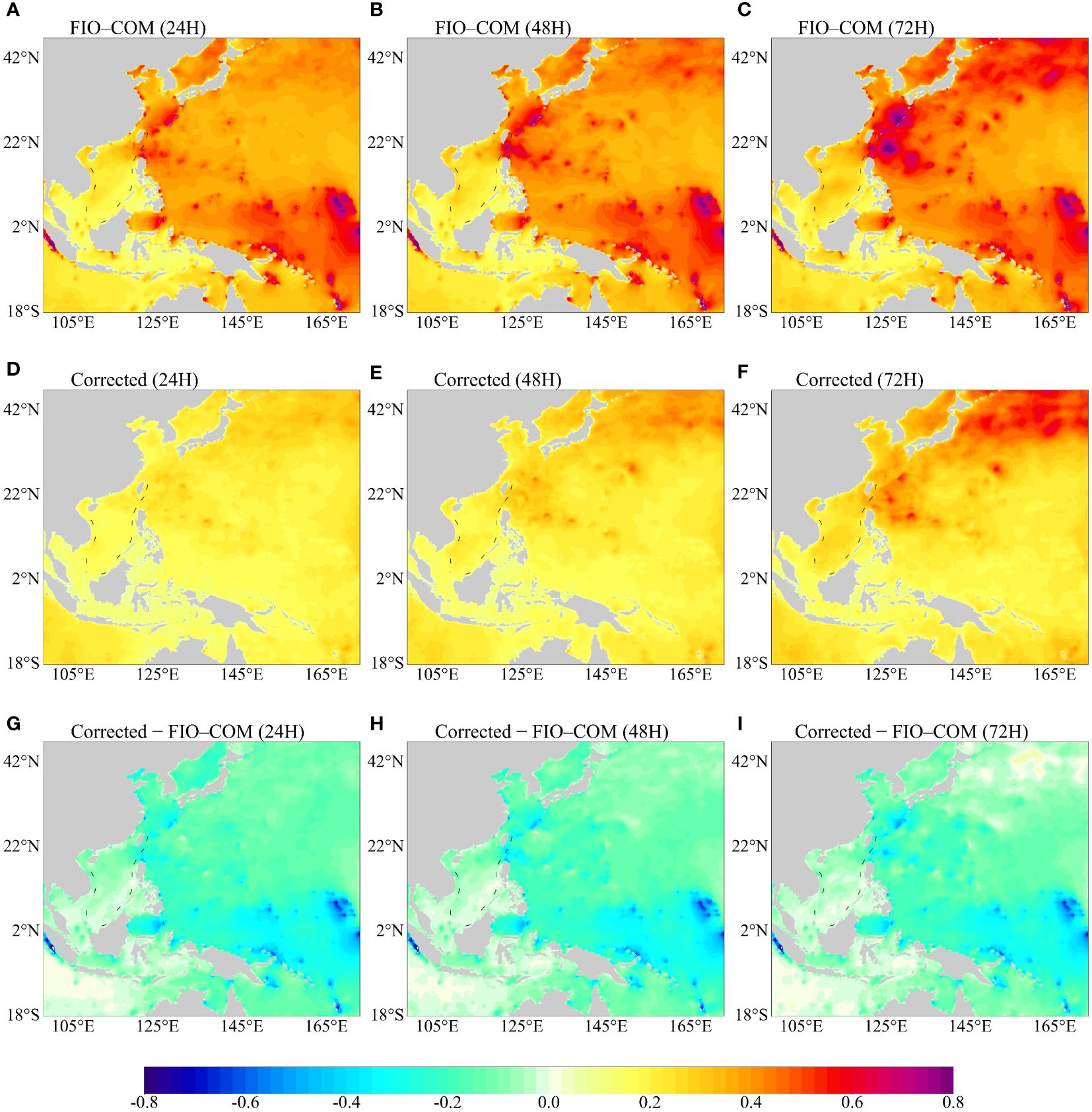
Figure 3 Spatial Distribution of RMSE (Units: m) for Forecast Intervals at 24, 48, and 72 hours. (A–C) depict RMSE skills of FIO-COM forecasts; (D–F) illustrate RMSE skills of post-corrected fields; (G–I) illustrate the difference of RMSE between Corrected and original fields. This figure provides a comparative visualization of the forecast accuracy before and after applying the correction methodology.

Further analysis of the corrected forecasts, as displayed in Figures 3D–F, reveals a continuous increase in RMSE with the extension of the forecast interval. This pattern suggests a marginal decrease in the effectiveness of the 2D-Geoformer correction over lengthier forecast durations. However, the spatial distribution of RMSE effectively highlights the 2D-Geoformer’s robustness in refining SWH forecasts across the entire study area. The most significant improvements are observed in regions where the original FIO-COM model exhibited higher errors, thereby emphasizing the 2D-Geoformer’s exceptional performance in areas with initial high forecasting inaccuracies. This comprehensive analysis underscores the 2D-Geoformer’s value in enhancing forecast accuracy and offers vital insights into its performance across varied spatial and temporal scales.

3.2 A case analysis of correction effects

While the RMSE effectively quantifies the overall performance of the FIO-COM numerical forecasting and the subsequent corrections applied through the 2D-Geoformer, it inherently lacks the capability to reflect the phase characteristics of the forecasting error. Specifically, RMSE does not discern whether the error in forecasting is an overestimation or underestimation relative to the actual observations. Consequently, to gain a more comprehensive understanding of the forecasting effectiveness, it becomes imperative to employ additional error statistical metrics and making further analysis.

Our analysis concentrates on a particular hindcasting case initiated on May. 26, 2023, at 12:00 UTC. The selection of this case is twofold: firstly, it exhibited the most pronounced correction effects throughout the entire testing period, making it an exemplary instance for detailed examination. Secondly, the case displays substantial variability in SWH, with values exceeding 8 meters in the open ocean southeast of Taiwan Island, compared to approximately 2 meters in other areas. This pronounced variation in wave heights present an ideal scenario to assess the model’s performance under diverse conditions. Figure 4 provides a visual comparison of the spatial distribution of SWH as forecasted by FIO-COM (Figures 4A–C) and as observed in the ERA5 reanalysis (Figures 4D–F). The similarities in patterns between the two indicate FIO-COM’s robust ability in capturing the spatial dynamics of SWH. However, a closer inspection reveals noticeable disparities between the FIO-COM SWH forecasts and the ERA5 reanalysis data. These disparities highlight areas where the model’s predictive accuracy can be further refined.

Figure 4

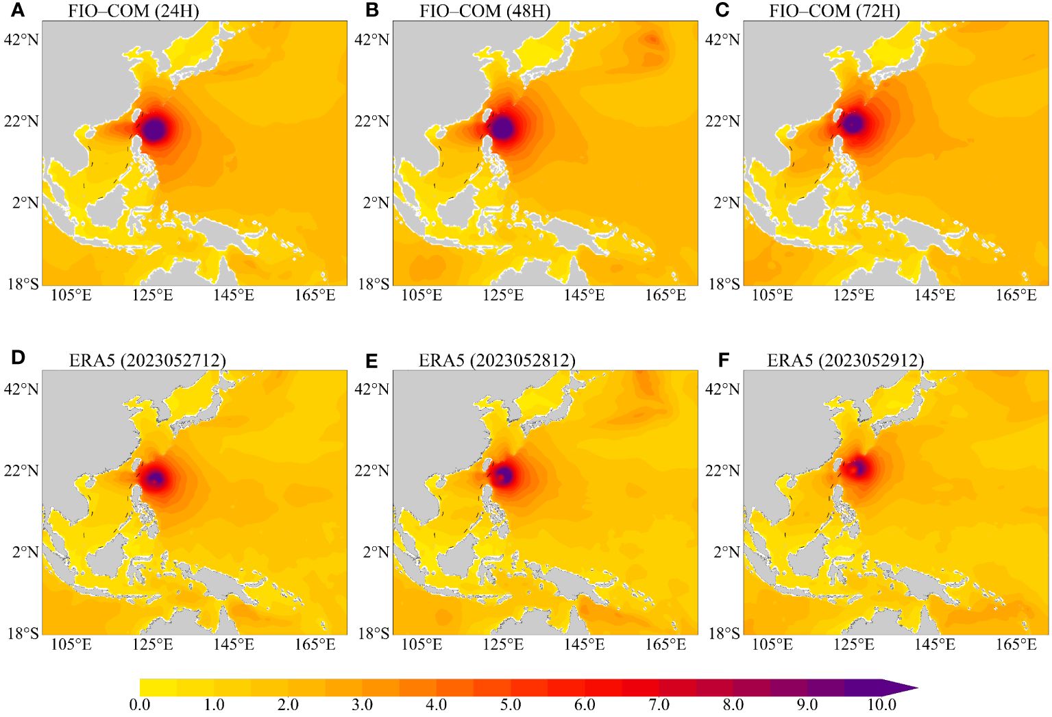
Figure 4 Illustration of the spatial distribution of SWH forecasts (Units: m) initiated on May 26, 2023, at 12:00 UTC. (A–C) display the SWH forecasts at 24, 48, and 72 hours, respectively. (D–F) correspond to the ERA5 reanalysis for the same intervals. This comparison provides insight into the model’s accuracy in capturing spatial variations in SWH over different forecast periods.

In this meticulous analysis of the specific forecasting case, it was observed that the FIO-COM model generally overestimates the SWH above 2 meters in the oceanic regions surrounding Taiwan island. Conversely, in most other areas, FIO-COM exhibits a slight overestimation tendency of approximately 0.5 meters. Notably, in the southwestern sectors of the study area, FIO-COM tends to underestimate the SWH (Figures 5A–C). The application of the 2D-Geoformer model in this context revealed an extraordinary capability to accurately retrieve the spatial distribution of these predictive errors. The patterns of both overestimation and underestimation errors, as identified by the 2D-Geoformer (Figures 5D–F), displayed remarkable alignment with those observed in the original FIO-COM forecasts, indicating the model’s precision in detecting discrepancies within the FIO-COM predictions.

Figure 5

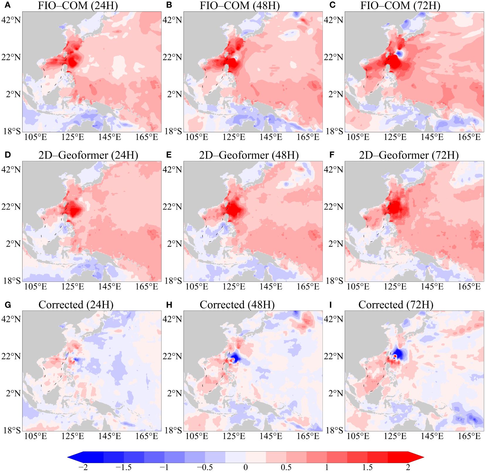
Figure 5 Depiction of Spatial Error Distribution (Units: m) in SWH Forecasts for case Commencing on May. 26, 2023, at 12:00 UTC. (A–C) illustrate the original SWH forecasting errors by the FIO-COM at 24, 48, and 72 hours. (D–F) present the error patterns retrieved by the 2D-Geoformer for the corresponding intervals. (G–I) showcase the corrected SWH errors post 2D-Geoformer adjustment for these respective time frames.

Upon applying the 2D-Geoformer’s error corrections to the FIO-COM SWH forecasts, the revised forecasts, as depicted in Figures 5G–I, demonstrated notable enhancements. A key observation was the substantial reduction of errors in most regions, particularly around the Taiwan islands, where errors decreased significantly from above 2 meters to approximately 0.5 meters. This improvement is especially significant given the tendency of the FIO-COM to produce large errors in conjunction with high SWH forecasts. Accurate SWH forecasting is crucial, especially in high-wave scenarios, due to its implications for maritime navigation and coastal management. High SWH conditions pose significant risks, underscoring the need for precision in forecasting. The effectiveness of our methodology in markedly reducing high SWH forecast errors within the FIO-COM is therefore invaluable for maritime and coastal applications. This pronounced decrease in error magnitude not only highlights the 2D-Geoformer’s capability in refining SWH forecast models but also emphasizes its critical role in enhancing maritime safety and operational efficiency.

An intriguing observation was noted in a small region to the east of the Taiwan islands, where the FIO-COM forecasts at 48 and 72 hours displayed negative values (Figures 5B, C), a detail that was not captured by the 2D-Geoformer (Figures 5E, F). This led to the corrective process exacerbating the original forecast errors in this region (Figures 5H, I). The underlying reason for this discrepancy lies in the 2D-Geoformer’s patch-based retrieving methodology. The inputs are divided into non-overlapping patches, each of size ($h_0\times w_0=4\times 4$), across the channel dimension, equating to a resolution of 2° by 2°. While the 2D-Geoformer excels in learning the overall characteristics between different patches and assigning average coefficients, it lacks the capability for finer analysis within individual patches. Therefore, for small regions with negative values surrounded by positive values, the 2D-Geoformer may overlook critical localized information.

We further evaluated the correction effects of the 2D-Geoformer at individual grid points by concurrently plotting the error distribution of the FIO-COM model and the reproduced error as determined by the 2D-Geoformer (Figure 6). In this graphical representation, the positioning of data points within the first and third quadrants indicates positive correction effects by the 2D-Geoformer on the FIO-COM forecasting errors. Closer proximity of these points to the diagonal line, which extends across the first and third quadrants, signifies a more robust and effective correction. Conversely, data points residing in the second and fourth quadrants suggest instances where the 2D-Geoformer may have inadvertently exacerbated the FIO-COM forecasting errors. A significant observation from this analysis is the 2D-Geoformer’s ability to accurately reproduce the FIO-COM forecasting errors, particularly in grid points characterized by high SWH errors. However, its effectiveness appears somewhat diminished in grids where the original FIO-COM forecasting errors are relatively minor. This pattern remains consistent across various forecasting periods, including 24, 48, and 72 hours (Figures 6A–C).

Figure 6

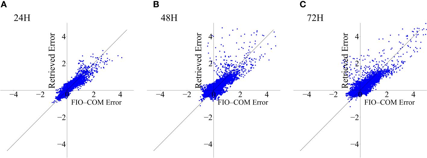
Figure 6 Comparative analysis of error (Units: m) distributions from FIO-COM forecasts and errors retrieved by the 2D-Geoformer across grid points for the case initiated on May 26, 2023, at 12:00 UTC. (A–C) illustrate the distributions at forecasting intervals of 24, 48, and 72 hours, respectively.

To rigorously quantify the correction effectiveness, an analysis was conducted to calculate the proportion of effectively corrected grids compared to the total number of grids, based on the varying magnitudes of FIO-COM forecasting errors (Table 2). For errors ranging between -0.5 and 0.5, the correction impact was moderate, with effectively corrected grid proportions at 59.6%, 51.1%, and 46.7% for the 24, 48, and 72-hour forecasting intervals, respectively. In cases of errors below -0.5, the correction was markedly more significant, resulting in 96.2%, 88.9%, and 77.9% of grids being effectively corrected for these respective intervals. Similarly, for errors exceeding 0.5, the correction was also substantial, with 98.4%, 96.8%, and 97.2% of grids effectively corrected for the same forecasting durations. This analysis highlights that grids with higher initial FIO-COM SWH forecasting errors predominantly underwent effective refinement following correction. Conversely, grids with lower initial errors exhibited a decreased rate of effective correction. The significance of these findings underscores the vital importance of accurate SWH forecasting, particularly in scenarios involving high SWH, due to its implications for maritime safety and operational planning.

Table 2

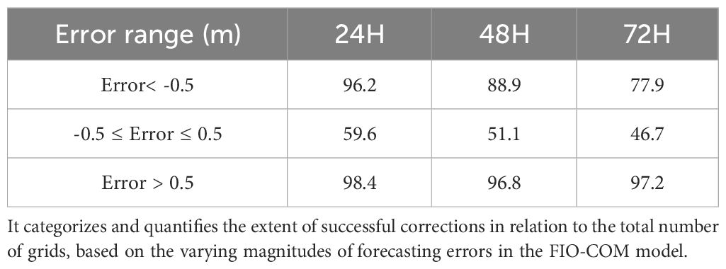
Table 2 The proportion (%) of effectively corrected grids in the FIO-COM forecasts for the case initiated on May 26, 2023, at 12:00 UTC, covering forecast intervals of 24, 48, and 72 hours.

4 Conclusion

The significance of accurate SWH forecasting is widely recognized due to its various applications. While wave numerical models have advanced significantly over the past decades, they still face considerable errors due to the incomplete representation of various physical processes. Deep learning methods have also progressed, mainly focusing on single-point forecasting; however, their effectiveness in spatial forecasting is not as prominent as that of numerical models. These deep learning approaches primarily seek to uncover internal regularities within SWH datasets, particularly the time-evolving characteristics, but often overlook the advancements in numerical modeling.

This paper introduces an innovative approach that amalgamates the latest developments in numerical wave forecasting and the adeptness of deep learning in identifying patterns within datasets. By designing a 2D-Geoformer deep learning model, we aim to elucidate the relationship between original numerical forecasting fields and their associated errors. Subsequently, this model identifies the numerical forecasting errors of SWH, which are then subtracted from the original forecasts to yield corrected SWH forecasts. Our findings reveal the remarkable effectiveness of this method in rectifying numerical SWH forecasting errors. Throughout the testing period, this approach consistently reduced the RMSE significantly compared to the original numerical forecasts. Particularly noteworthy is the refinement of SWH forecasts in most grids, especially those with initially high SWH numerical forecasting errors.

By amalgamating numerical advancements with deep learning techniques, this approach significantly advances beyond traditional SWH forecasting methods, which generally depend solely on either numerical models or deep learning frameworks. However, the present study predominantly assesses the FIO-COM numerical forecasting model within a constrained research scope. Future investigations are warranted to ascertain the effectiveness of this methodology across a wider array of domains and with various SWH forecasting models. Moreover, expanding this method’s application to global oceans will require overcoming computational challenges and refining the 2D-Geoformer model to boost its efficiency. It is also pertinent to highlight that this research employs ERA5 reanalysis datasets as the observational benchmark. Although ERA5 reanalysis SWH data serve as a robust surrogate for actual observations, they are not devoid of errors. Subsequent studies should consider the incorporation of data from diverse sources to improve observational precision. Additionally, the current investigation utilizes the 2D-Geoformer, a statistically based method; future endeavors could explore physically based deep learning techniques (Xu et al., 2021; Sun et al., 2022; Jiang et al., 2023; Wang and Huang, 2024), potentially yielding more robust outcomes. In conclusion, the methodologies delineated in this study are crucial for the progression of SWH forecasting, providing significant advantages for maritime navigation, coastal management, and the broader spectrum of marine economic activities.

Data availability statement

The raw data supporting the conclusions of this article will be made available by the authors, without undue reservation.

Author contributions

XK: Supervision, Conceptualization, Writing – review & editing, Writing – original draft, Funding acquisition. HS: Methodology, Writing – review & editing, Writing – original draft. ZZ: Writing – original draft, Software, Methodology, Formal analysis. XY: Writing – review & editing, Supervision, Formal analysis, Conceptualization. JG: Writing – original draft, Visualization, Validation

Funding

The author(s) declare financial support was received for the research, authorship, and/or publication of this article. This research was supported financially by Laoshan Laboratory (LSKJ202202103), the Fundamental Research Funds for the Central Universities (Grant No. JG2022-24), Open Foundation of Key Laboratory of Marine Science and Numerical Simulation, Ministry of Natural Resources (Grant No. 2021-YB-02), and National Natural Science Foundation of China (Grant No. 42205157).

Acknowledgments

We acknowledge Dr. Lu Zhou for the foundational 3D-Geoformer codes (https://github.com/zhoulu327/Code_of_3D-Geoformer/commits/v1.0). These codes provided a critical starting point for our research. Building upon this preliminary framework, we have meticulously adapted and refined the original 3D-Geoformer architecture, tailoring it specifically to meet the unique requirements and challenges inherent in 2D SWH error correction.

Conflict of interest

The authors declare that the research was conducted in the absence of any commercial or financial relationships that could be construed as a potential conflict of interest.

Publisher’s note

All claims expressed in this article are solely those of the authors and do not necessarily represent those of their affiliated organizations, or those of the publisher, the editors and the reviewers. Any product that may be evaluated in this article, or claim that may be made by its manufacturer, is not guaranteed or endorsed by the publisher.

Supplementary material

The Supplementary Material for this article can be found online at: https://www.frontiersin.org/articles/10.3389/fmars.2024.1374902/full#supplementary-material

References

Allahdadi M. N., Gunawan B., Lai J., He R., Neary V. S. (2019). Development and validation of a regional-scale high-resolution unstructured model for wave energy resource characterization along the US East Coast. Renewable Energy 136, 500–511. doi: 10.1016/j.renene.2019.01.020

CrossRef Full Text | Google Scholar

Altunkaynak A. (2015). Prediction of significant wave height using spatial function. Ocean Eng. 106, 220–226. doi: 10.1016/j.oceaneng.2015.06.028

CrossRef Full Text | Google Scholar

Amarouche K., Akpinar A., Rybalko A., Myslenkov S. (2023). Assessment of SWAN and WAVEWATCH-III models regarding the directional wave spectra stimates based on Eastern Black Sea measurements. Ocean Eng. 272, 113944. doi: 10.1016/j.oceaneng.2023.113944

CrossRef Full Text | Google Scholar

Bennis A.-C., Furgerot L., Du Bois P. B., Dumas F., Odaka T., Lathuiliere C., et al. (2020). Numerical modelling of three-dimensional wave-current interactions in complex environment: application to Alderney Race. Appl. Ocean Res. 95, 102021. doi: 10.1016/j.apor.2019.102021

CrossRef Full Text | Google Scholar

Bertasius G., Wang H., Torresani L. (2021). Is space-time attention all you need for video understanding? In ICML 2(3), 4. doi: 10.48550/arXiv.2102.05095

CrossRef Full Text | Google Scholar

Bitner-Gregersen E. M., Waseda T., Parunov J., Yim S., Hirdaris S., Ma N., et al. (2022). Uncertainties in long-term wave modelling. Mar. Structures 84, 103217. doi: 10.1016/j.marstruc.2022.103217

CrossRef Full Text | Google Scholar

Booij N., Ris R. C., Holthuijsen L. H. (1999). A third-generation wave model for coastal regions: 1. Model description and validation. J. Geophys. Res. 104, 7649–7666. doi: 10.1029/98JC02622

CrossRef Full Text | Google Scholar

Çelik A. (2022). Improving prediction performance of significant wave height via hybrid SVD-Fuzzy model. Ocean Eng. 266, 113173. doi: 10.1016/j.oceaneng.2022.113173

CrossRef Full Text | Google Scholar

Choi H., Park M., Son G., Jeong J., Park J., Mo K., et al. (2020). Real-time significant wave height estimation from raw ocean images based on 2D and 3D deep neural networks. Ocean Eng. 201, 107129. doi: 10.1016/j.oceaneng.2020.107129

CrossRef Full Text | Google Scholar

Demetriou D., Michailides C., Papanastasiou G., Onoufriou T. (2021). Nowcasting significant wave height by hierarchical machine learning classification. Ocean Eng. 242, 110130. doi: 10.1016/j.oceaneng.2021.110130

CrossRef Full Text | Google Scholar

Elbisy M. S., Elbisy A. M. S. (2021). Prediction of significant wave height by artificial neural networks and multiple additive regression trees. Ocean Eng. 230, 109077. doi: 10.1016/j.oceaneng.2021.109077

CrossRef Full Text | Google Scholar

Fan S., Xiao N., Dong S. (2020). A novel model to predict significant wave height based on long short-term memory network. Ocean Eng. 205, 107298. doi: 10.1016/j.oceaneng.2020.107298

CrossRef Full Text | Google Scholar

Fernández J. C., Salcedo-Sanz S., Gutiérrez P. A., Alexandre E., Hervás-Martínez C. (2015). Significant wave height and energy flux range forecast with machine learning classifiers. Eng. Appl. Artif. Intell. 43, 44–53. doi: 10.1016/j.engappai.2015.03.012

CrossRef Full Text | Google Scholar

Group T. W. (1988). The WAM model—A third generation ocean wave prediction model. J. Phys. Oceanography 18, 1775–1810. doi: 10.1175/1520-0485(1988)018<1775:TWMTGO>2.0.CO;2

CrossRef Full Text | Google Scholar

Han L., Ji Q., Jia X., Liu Y., Han G., Lin X. (2022). Significant wave height prediction in the south China sea based on the convLSTM algorithm. J. Mar. Sci. Eng. 10, 1683. doi: 10.3390/jmse10111683

CrossRef Full Text | Google Scholar

Hersbach H., Bell B., Berrisford P., Hirahara S., Horányi A., Muñoz-Sabater J., et al. (2020). The ERA5 global reanalysis. Quart J. R. Meteoro Soc. 146, 1999–2049. doi: 10.1002/qj.3803

CrossRef Full Text | Google Scholar

Jiang T. T., Fang L., Wang K. (2023). Deciphering “the language of nature”: A transformer-based language model for deleterious mutations in proteins. Innovation 4(5), 100487. doi: 10.1016/j.xinn.2023.100487

CrossRef Full Text | Google Scholar

Kaloop M. R., Kumar D., Zarzoura F., Roy B., Hu J. W. (2020). A wavelet - Particle swarm optimization - Extreme learning machine hybrid modeling for significant wave height prediction. Ocean Eng. 213, 107777. doi: 10.1016/j.oceaneng.2020.107777

CrossRef Full Text | Google Scholar

Kumar N. K., Savitha R., Mamun A. A. (2017). Regional ocean wave height prediction using sequential learning neural networks. Ocean Eng. 129, 605–612. doi: 10.1016/j.oceaneng.2016.10.033

CrossRef Full Text | Google Scholar

Lionello P., Günther H., Janssen P. (1992). Assimilation of altimeter data in a global third-generation wave model. J. Geophysical Res. 971, 14453–14474. doi: 10.1029/92JC01055

CrossRef Full Text | Google Scholar

Muhammed Naseef T., Sanil Kumar V. (2020). Climatology and trends of the Indian Ocean surface waves based on 39-year long ERA5 reanalysis data. Intl J. Climatology 40, 979–1006. doi: 10.1002/joc.6251

CrossRef Full Text | Google Scholar

Oh J., Suh K.-D. (2018). Real-time forecasting of wave heights using EOF – wavelet – neural network hybrid model. Ocean Eng. 150, 48–59. doi: 10.1016/j.oceaneng.2017.12.044

CrossRef Full Text | Google Scholar

Pirhooshyaran M., Snyder L. V. (2020). Forecasting, hindcasting and feature selection of ocean waves via recurrent and sequence-to-sequence networks. Ocean Eng. 207, 107424. doi: 10.1016/j.oceaneng.2020.107424

CrossRef Full Text | Google Scholar

Ponce De León S., Bettencourt J., Van Vledder G., Doohan P., Higgins C., Guedes Soares C., et al. (2018). “Performance of WAVEWATCH-III and SWAN models in the north sea,” in Volume 11B: Honoring Symposium for Professor Carlos Guedes Soares on Marine Technology and Ocean Engineering (American Society of Mechanical Engineers, Madrid, Spain), V11BT12A052. doi: 10.1115/OMAE2018-77291

CrossRef Full Text | Google Scholar

Qiao F., Wang G., Khokiattiwong S., Akhir M. F., Zhu W., Xiao B. (2019). China published ocean forecasting system for the 21st-Century Maritime Silk Road on December 10, 2018, Acta Oceanologica Sinica= Hai Yang Hsueh Pao, 38(1), 1–3. doi: 10.1007/s13131-019-1365-y

CrossRef Full Text | Google Scholar

Qiao F., Zhao W., Yin X., Huang X., Liu X., Shu Q., et al. (2016). “A highly effective global surface wave numerical simulation with ultra-high resolution,” in Proceedings of the International Conference for High Performance Computing, Networking, Storage and Analysis SC ‘16 (IEEE Press, Salt Lake City, Utah), 1–11. doi: 10.1109/SC.2016.4

CrossRef Full Text | Google Scholar

Qiu S., Liu K., Wang D., Ye J., Liang F. (2019). A comprehensive review of ocean wave energy research and development in China. Renewable Sustain. Energy Rev. 113, 109271. doi: 10.1016/j.rser.2019.109271

CrossRef Full Text | Google Scholar

Ris R. C., Holthuijsen L. H., Booij N. (1999). A third-generation wave model for coastal regions: 2. Verification. J. Geophys. Res. 104, 7667–7681. doi: 10.1029/1998JC900123

CrossRef Full Text | Google Scholar

Saavedra V., Montoya R., Orfila A., AndrésF O. (2023). Assimilation of peak period from video images in numerical wave models at a local scale. Comput. Geosciences, 178, 105407. doi: 10.1016/j.cageo.2023.105407

CrossRef Full Text | Google Scholar

Shi H., Cao X., Li Q., Li D., Sun J., You Z.-J., et al. (2021). Evaluating the accuracy of ERA5 wave reanalysis in the water around China. J. Ocean Univ. China 20, 1–9. doi: 10.1007/s11802-021-4496-7

CrossRef Full Text | Google Scholar

Shi J., Su T., Li X., Wang F., Cui J., Liu Z., et al. (2023). A machine-learning approach based on attention mechanism for significant wave height forecasting. J. Mar. Sci. Eng. 11, 1821. doi: 10.3390/jmse11091821

CrossRef Full Text | Google Scholar

Song T., Han R., Meng F., Wang J., Wei W., Peng S. (2022). A significant wave height prediction method based on deep learning combining the correlation between wind and wind waves. Front. Mar. Sci. 9. doi: 10.3389/fmars.2022.983007

PubMed Abstract | CrossRef Full Text | Google Scholar

Sun X., Yang Y., Jia H., Yang J. (2022). Physics-aware training for the physical machine learning model building. Innovation 3 (5), 100287. doi: 10.1016/j.xinn.2022.100287

PubMed Abstract | CrossRef Full Text | Google Scholar

Takbash A., Young I. (2020). Long-term and seasonal trends in global wave height extremes derived from ERA-5 reanalysis data. JMSE 8, 1015. doi: 10.3390/jmse8121015

CrossRef Full Text | Google Scholar

Tolman H. L. (2009). User manual and system documentation of WAVEWATCH III TM version 3.14. Tech. note MMAB Contribution 276(220).

Google Scholar

Vaswani A., Shazeer N., Parmar N., Uszkoreit J., Jones L., Gomez A. N., et al. (2017). "Attention is all you need." Advances in neural information processing systems, 30.

Google Scholar

Wang H., Fu D., Liu D., Xiao X., He X., Liu B. (2021). Analysis and prediction of significant wave height in the beibu gulf, south China sea. JGR Oceans 126, e2020JC017144. doi: 10.1029/2020JC017144

CrossRef Full Text | Google Scholar

Wang T., Huang P. (2024). Superiority of a convolutional neural network model over dynamical models in predicting central pacific ENSO. Adv. Atmos. Sci. 41, 141–154. doi: 10.1007/s00376-023-3001-1

CrossRef Full Text | Google Scholar

Wang J., Wang Y. (2022). Evaluation of the ERA5 significant wave height against NDBC buoy data from 1979 to 2019. Mar. Geodesy 45, 151–165. doi: 10.1080/01490419.2021.2011502

CrossRef Full Text | Google Scholar

Wang G., Zhao C., Xu J., Qiao F., Xia C. (2016). Verification of an operational ocean circulation-surface wave coupled forecasting system for the China’s seas. Acta Oceanologica Sin. 35, 19–28. doi: 10.1007/s13131-016-0810-4

CrossRef Full Text | Google Scholar

Xiao B., Qiao F., Shu Q., Yin X., Wang G., Wang S. (2023). Development and validation of a global 1/32° surface-wave–tide–circulation coupled ocean model: FIO-COM32. Geoscientific Model. Dev. 16, 1755–1777. doi: 10.5194/gmd-16-1755-2023

CrossRef Full Text | Google Scholar

Xu Y., Liu X., Cao X., Huang C., Liu E., Qian S., et al. (2021). Artificial intelligence: A powerful paradigm for scientific research. Innovation 2, 100179. doi: 10.1016/j.xinn.2021.100179

PubMed Abstract | CrossRef Full Text | Google Scholar

Yong-zeng Y., Fang-li Q., Wei Z., Yong T., Ye-li Y. (2005). MASNUM ocean wave numerical model in spherical coordinates and its application. Acta Oceanologica Sin. 27, 1–7.

Google Scholar

Zhang W.-W. (2012). The China wave: Rise of a civilizational state (World Scientific). Singapore. doi: 10.1142/9781938134029

CrossRef Full Text | Google Scholar

Zhang X., Li Y., Gao S., Ren P., Lara J. L. (2021). Ocean wave height series prediction with numerical long short-term memory. J. Mar. Sci. Eng. 9(5), 514. doi: 10.3390/jmse9050514

CrossRef Full Text | Google Scholar

Zhang D., Li W., Lin Y. (2009). Wave energy in China: Current status and perspectives. Renewable Energy 34, 2089–2092. doi: 10.1016/j.renene.2009.03.014

CrossRef Full Text | Google Scholar

Zhao W., Song Z., Qiao F., Yin X. (2014). High efficient parallel numerical surface wave model based on an irregular quasi-rectangular domain decomposition scheme. Sci. China Earth Sci. 57, 1869–1878. doi: 10.1007/s11430-014-4842-3

CrossRef Full Text | Google Scholar

Zheng C., Zhu S., Mendieta M., Yang T., Chen C., Ding Z. (2021). “3D human pose estimation with spatial and temporal transformers,” in 2021 IEEE/CVF International Conference on Computer Vision (ICCV) (IEEE, Montreal, QC, Canada), 11636–11645. doi: 10.1109/ICCV48922.2021.01145

CrossRef Full Text | Google Scholar

Zhou S., Bethel B. J., Sun W., Zhao Y., Xie W., Dong C. (2021). Improving significant wave height forecasts using a joint empirical mode decomposition–long short-term memory network. JMSE 9, 744. doi: 10.3390/jmse9070744

CrossRef Full Text | Google Scholar

Zhou L., Zhang R.-H. (2023). A self-attention–based neural network for three-dimensional multivariate modeling and its skillful ENSO predictions. Sci. Adv. 9, eadf2827. doi: 10.1126/sciadv.adf2827

PubMed Abstract | CrossRef Full Text | Google Scholar

Zilong T., Yubing S., Xiaowei D. (2022). Spatial-temporal wave height forecast using deep learning and public reanalysis dataset. Appl. Energy 326, 120027. doi: 10.1016/j.apenergy.2022.120027

CrossRef Full Text | Google Scholar